Article

Parameter Compensation for the Predictive Control System of a Permanent Magnet Synchronous Motor Based on Bacterial Foraging Optimization Algorithm

1
IoT Technology Application Engineering Research Center of the Ministry of Education, Jiangnan University, Wuxi 214122, China
2
Nanjing Power Supply Branch of State Grid Jiangsu Electric Power Co., Ltd., Nanjing 210019, China
*
Author to whom correspondence should be addressed.
World Electr. Veh. J. 2024, 15(1), 23; https://doi.org/10.3390/wevj15010023
Submission received: 7 November 2023 / Revised: 13 December 2023 / Accepted: 27 December 2023 / Published: 9 January 2024
(This article belongs to the Special Issue Permanent Magnet Motors and Driving Control for Electric Vehicles)

Abstract

:
The accurate identification of permanent magnet synchronous motor (PMSM) parameters is the foundation for high-performance driving in predictive control systems. The traditional PMSM multi-parameter identification method suffers from insufficient rank of the identification equation and is prone to getting stuck in local optimal solutions. This article combines the bacterial foraging optimization algorithm (BFOA) to establish a built-in PMSM predictive control parameter compensation model. Firstly, we analyzed the reasons why the distortion of PMSM motor parameters affects the actual speed and calculated the deviation of d-axis and q-axis currents caused by the distortion. Secondly, parameter compensation was applied to the prediction model, and BFOA was combined to optimize the compensation parameters. This algorithm does not use the traditional voltage equation as the fitness function but instead uses a brand-new set of four equations for parameter iteration optimization. The optimized compensation parameters can reduce current deviation and improve the robustness of the PMSM predictive control system. The proposed model can cover four kinds of motor distortion parameters, including stator resistance, D-axis inductance, Q-axis inductance, and permanent magnet flux linkage. Finally, the traditional PMSM predictive control model is compared with the predictive control model combined with BFOA. The simulation results show that the dynamic and static performance of the compensated system is improved when single or multiple parameters are distorted.

1. Introduction

In response to the call of the National Development and Reform Commission’s “14th Five-Year Plan for Modern Energy System”, vigorously developing new energy technologies has become the only way for China to move from a major automobile country to a strong automobile country [1]. As the main actuator of new energy vehicles, the performance of the drive motor determines their core performance [2]. In order to meet the power requirements for starting, accelerating, driving, decelerating, and braking a car, it is often required that the vehicle motor have a wide range of speed regulation performance and high dynamic performance. In addition, the motor should have high resistance to temperature and humidity, low noise during operation, and be able to work for a long time under harsh environmental conditions. PMSM is often used as a driving motor for electric vehicles due to its advantages such as lightweight, small size, high-power density, and strong reliability [3,4,5].
Due to PMSM being a complex, nonlinear, strongly coupled, and multivariable system, its control is difficult and costly. Among numerous PMSM control systems, Finite Control Set Model Predictive Current Control (FCS-MPCC) stands out due to its low model requirements, good control quality, and convenient online calculation [6,7,8]. However, FCS-MPCC still has obvious drawbacks in practical applications: the physical structure of PMSM has tooth slot effect, edge effect, and saturation effect, and there will be temperature rise parameter changes during operation. The prediction results depend on the system model parameters, and parameter mismatches can lead to a decrease in control performance [9]. Therefore, in order to further enhance the development and application of PMSM in the field of electric vehicles, research on the parameter robustness of PMSM predictive control systems has become a current hot topic.
There are two types of research on robustness issues. One method is online parameter recognition, which is based on real-time recognition of parameter changes, substituting the true values of parameters into the control system to improve control accuracy [10,11]. At present, commonly used online parameter identification methods include the least squares method [12], extended Kalman filter [13], and model reference adaptive method [14,15]. The objective function of the least squares method is simple, with a minimum objective function value of zero, and the computational workload is moderate. However, in the optimization process under non-stationary conditions, the tracking ability of the objective function is poor and more sensitive to external disturbances. In addition, due to the need to simplify the model and linearize the parameters, this method may lead to a decrease in identification accuracy. An extended Kalman filter is an extension of the Kalman filter in nonlinear system applications that can provide state estimation in the sense of minimum variance for nonlinear systems in noisy environments. However, it is necessary to process the parameters to be identified into state variables, which requires complex matrix and vector operations and makes it difficult to design algorithms for multi-parameter measurement. The basic idea of the model reference adaptive algorithm is to use the motor body as the reference model and the equation system containing the parameters to be identified as the adjustable model. Under the same excitation input, two models have the same physical output. Identify parameters when the error approaches zero by combining the output error between two models and an adaptive law designed based on Lyapunov theory or Popov theory. This algorithm has a simple structure and easy convergence of results, but it is difficult to use for multi-parameter identification/measurement of missing ranks. In fact, in the multi-parameter identification of permanent magnet synchronous motors, these traditional identification methods generally have the problem of insufficient rank. The number of unknown parameters to be identified exceeds the number of control system equations, resulting in multiple sets of identification results with significant errors. Therefore, Zhou et al. [16] solved the multi-parameter discrimination problem under rank deficiency by constructing a second-order steady-state equation. Yu et al. [17] used the voltage equation on the shaft to construct an equal rank equation to estimate the entire motor parameters in both steady-state and transient states. Zhang et al. [18] and Feng et al. [19] both proposed a method of injecting a d-axis negative sequence current in a short period of time, which effectively solves the problem of insufficient sorting of the mathematical model of permanent magnet synchronous motors and can quickly achieve simultaneous identification of multiple parameters. However, whether constructing equal rank equations using different states of the motor or solving rank problems by injecting current into the d-axis, both increase the operational complexity of parameter identification and limit its application in the industrial field. If a set of equal rank equations that can be identified without additional operations can be found, it will greatly simplify the identification process.
Another method to improve system robustness is biomimetic intelligent optimization algorithms. This method uses regularly measured data and correctly defined objective functions, providing an ideal automation solution for parameter estimation in permanent magnet synchronous motor systems. Especially the Particle Swarm Optimization (PSO) algorithm, which is a naturally inspired algorithm with advantages such as simple implementation and parallel search in the solution space, has strong capabilities in handling multivariate parameter optimization problems. This algorithm has been widely used in the parameter estimation of motors [20,21,22]. For example, in [21], a coevolutionary PSO combined with an artificial immune system (AIS) was developed to improve the estimation performance of PMSM multiple parameters using the designed objective function. In order to accelerate the search process of the group, some parallel improved PSO algorithms have been proposed for parameter estimation and temperature monitoring of PMSM; ref. [22] proposed a dynamic PSO with a learning strategy and designed a novel motion correction equation with variable exploration vectors to effectively update particles, enabling the population to cover a large area of search with a high probability. This PSO is effective in estimating the stator resistance and rotor flux of permanent magnet synchronous motors, or d-axis inductance and q-axis inductance, but it cannot satisfactorily estimate all machine parameters simultaneously, because when dealing with time-varying multi-parameter optimization problems, PSO is prone to getting stuck in local minima. In addition, the existing parameter estimation of permanent magnet synchronous motors based on particle swarm optimization algorithms is mainly focused on surface-mounted permanent magnet synchronous motors, and there is little research on built-in permanent magnet synchronous motors. Due to the fact that the quadrature axis inductance of the built-in permanent magnet synchronous motor is greater than the direct axis inductance, its mathematical model is more complex compared to the surface-mounted synchronous motor. However, the built-in rotor structure can fully utilize the reluctance torque generated by the asymmetry of the rotor magnetic circuit, improve the power density of the motor, and improve the dynamic performance of the motor compared to the surface-mounted rotor structure. Therefore, it is necessary to conduct research on intelligent algorithm parameter identification for built-in permanent magnet synchronous motors.
In order to achieve the design and safe operation of a high-performance predictive control system for permanent magnet synchronous motors, comprehensive modeling work is always necessary, which accurately identifies the motor’s resistance, d-axis inductance, q-axis inductance, and magnetic flux. In view of the above situation, this article innovates from three aspects: principle, method, and object, and proposes a parameter compensation method for the PMSM predictive control system based on the Bacteria Feeding Optimization Algorithm (BFOA). In terms of principle, in order to solve the problem of missing rank in parameter identification equations, this paper proposes four new fitness functions for parameter identification without the need to construct additional transient or steady-state equations and without injecting current into the d-axis. At the method level, in order to solve the problem of PSO easily falling into local minima, BFOA is used for intelligent search. BFOA is an intelligent optimization algorithm proposed to solve problems such as complexity, nonlinearity, and constraints in large-scale optimization events. Compared to PSO, the decentralized stage of BFOA gives it super strong global search ability [23,24,25], avoiding the problem of getting stuck in local minima during the search process. At the level of the target audience, this article focuses on the research on surface-mounted permanent magnet synchronous motors. The specific steps can be divided into: firstly, using the formula to derive and analyze, and proposing four identification equations to reduce the predicted current deviation; secondly, using the BFOA algorithm to iteratively optimize parameters under the full rank identification equation; and finally, the optimized parameters will be compensated in the control system.
The structure of the article is as follows: Section 1 briefly introduces the working principle of the FCS-MPCC system; Section 2 analyzes the deviation of predicting current under parameter distortion and derives a new identification equation to reduce the deviation; Section 3 introduces the process of implementing parameter identification using BFOA; and Section 4 builds comparative simulation experiments to verify the feasibility and effectiveness of the proposed method. Section 5 summarizes the article and provides prospects for future research directions.

2. FCS-MPCC Theory and Model
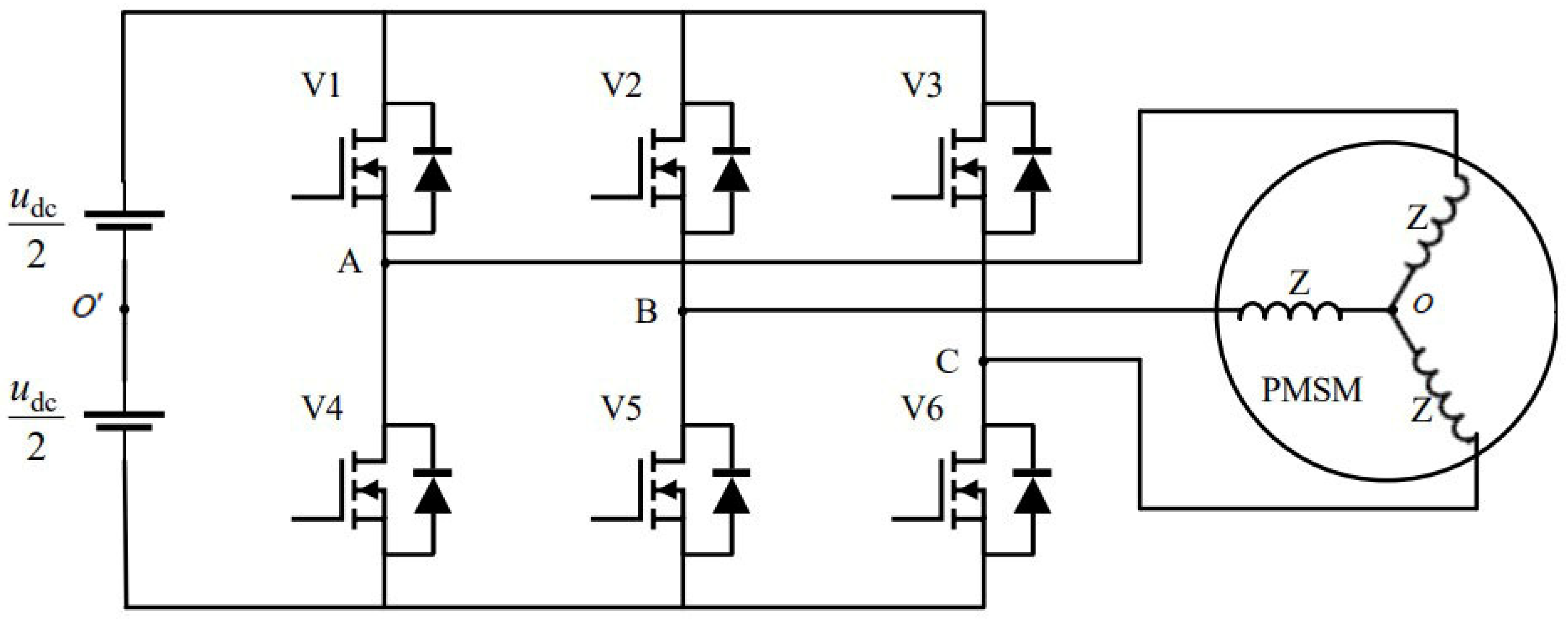
In 1983, predictive control was first extended and applied to motor drive systems by Professor Holtz, who proposed the method of Model Predictive Control (MPC) [26]. FCS-MPCC is developed from the classic MPC, which analyzes the current system state values, and the system state model selects the optimal predictive value after traversing and selecting finite control variables. It is widely used due to its advantages, such as its wide adaptability.

2.1. PMSM Model

The voltage of the PMSM three-phase winding is composed of stator resistance voltage and flux-induced voltage. The voltage equation in the three-phase stationary coordinate system is as follows:
u a = R s i a + d ψ a d t
u b = R s i b + d ψ b d t
u c = R s i c + d ψ c d t
By applying the Clark and Park transformations to the above three equations, the voltage equation in the d-q rotating coordinate system can be obtained:
u d = R s i d + d ψ d d t ω e ψ q
u q = R s i q + d ψ q d t + ω e ψ d
The magnetic linkage equation of PMSM in the d-q rotating coordinate system is as follows:
ψ d = L d i d + ψ f
ψ q = L q i q
By introducing Equations (6) and (7) into Equations (4) and (5), the voltage equation can be obtained as follows:
u d = R s i d + L d d i d d t L q ω e i q
u q = R s i q + L q d i q d t + L d ω e i d + ω e ψ f

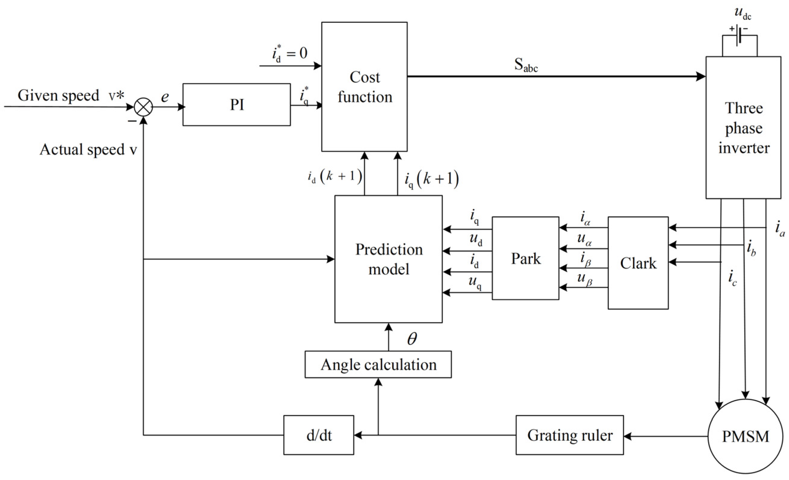
2.2. FCS-MPCC Theory

Write in Equations (8) and (9):
d i d d t = i d ( k + 1 ) i d ( k ) T
d i q d t = i q ( k + 1 ) i q ( k ) T
By introducing Equations (10) and (11) into Equations (8) and (9), the FCS-MPCC model can be derived:
i d ( k + 1 ) = ( 1 T R s L d ) i d ( k ) + T L d u d ( k ) + L q T ω e ( k ) L d i q ( k )
i q ( k + 1 ) = ( 1 T R s L q ) i q ( k ) + T L q u q ( k ) L d T ω e ( k ) L q i d ( k ) T ω e ( k ) ψ f L q
In the three-phase bridge inverter circuit that provides voltage to the motor, as shown in Figure 1. Different switch states can result in different three-phase stator voltages, as follows:
u a b c = S w ( : , i ) × u dc u dc 2
By transforming the coordinates of the three-phase voltages under different switching states, the d- and q-axis voltages under different switching states can be obtained, which are then incorporated into the predictive control model Equations (12) and (13). The obtained d-and q-axis predictive currents are then incorporated into the cost function:
J = [ ( i d ( k + 1 ) i d r e f ) 2 + ( i q ( k + 1 ) i q r e f ) 2 ]
The switch state at which the cost function is minimized is determined by the control system.

3. Analysis and Compensation of Parameter Distortion

When the PMSM predictive control system is actually running, motor parameters often undergo distortion due to changes in temperature, load, and external disturbances. The specific parameters of the motor include stator resistance R s , d-axis inductance L d , q-axis inductance L q , and permanent magnet flux ψ f . These distorted parameters can cause deviations in the predicted current, which in turn affects the speed performance of the motor.

3.1. Predicted Current Deviation

The motor prediction model is as follows:
i d p ( k + 1 ) = i d ( k ) + T L dm [ u d ( k ) R m i d ( k ) + L qm ω e ( k ) i q ( k ) ]
i q p ( k + 1 ) = i q ( k ) + T L qm [ u q ( k ) R m i q ( k ) L dm ω e ( k ) i d ( k ) ψ fm ω e ( k ) ]
The actual model with parameter mismatch is as follows:
i d a ( k + 1 ) = i d ( k ) + T L da [ u d ( k ) R a i d ( k ) + L qa ω e ( k ) i q ( k ) ]
i q a ( k + 1 ) = i q ( k ) + T L qa [ u q ( k ) R a i q ( k ) L da ω e ( k ) i d ( k ) ψ fa ω e ( k ) ]
and
L da = L dm + Δ L d
L qa = L qm + Δ L q
R a = R m + Δ R
ψ fa = ψ fm + Δ ψ
The deviation of d-axis and q-axis current caused by parameter distortion is as follows:
i d p ( k + 1 ) i d a ( k + 1 ) = T L dm ( L dm + Δ L d ) { [ u d ( k ) R m i d ( k ) + L qm ω e ( k ) i q ( k ) ] Δ L d [ L dm ω e ( k ) i q ( k ) ] Δ L q + [ L dm i d ( k ) ] Δ R }
i q p ( k + 1 ) i q a ( k + 1 ) = T L qm ( L qm + Δ L q ) { [ u q ( k ) R m i q ( k ) L dm ω e ( k ) i d ( k ) ψ fm ω e ( k ) ] Δ L q + [ L qm ω e ( k ) i d ( k ) ] Δ L d + [ L qm i q ( k ) ] Δ R + [ L qm ω e ( k ) ] Δ ψ }
The existence of a predicted current bias causes a shift in the switching state of the inverter circuit selection. In order to improve system robustness, it is particularly important to weaken the magnitude of the current bias.

3.2. Parameter Compensation

To reduce the predicted current deviation, the prediction model is compensated:
i dc p ( k + 1 ) = i d ( k ) + T L dm + Δ L d [ u d ( k ) ( R m + Δ R ) i d ( k ) + ( L qm + Δ L q ) ω e ( k ) i q ( k ) ]
i qc p ( k + 1 ) = i q ( k ) + T L qm + Δ L q [ u q ( k ) ( R m + Δ R ) i q ( k ) ( L dm + Δ L d ) ω e ( k ) i d ( k ) ( ψ fm + Δ ψ ) ω e ( k ) ]
At this point, the predicted current deviation after compensation is as follows:
i dc p ( k + 1 ) i d a ( k + 1 ) = d e v d 1 + d e v d 2
The superscripts 1 and 2 indicate the deviation component labels and have no practical significance.
d e v d 1 = T ( L dm + Δ L d ) ( L dm + Δ L d ) { [ u d ( k ) ( R m + Δ R ) i d ( k ) + ( L qm + Δ L q ) ω e ( k ) i q ( k ) ] Δ L d [ ( L dm + Δ L d ) ω e ( k ) i q ( k ) ] Δ L q + [ ( L dm + Δ L d ) i d ( k ) ] Δ R }
d e v d 2 = T ( L dm + Δ L d ) ( L dm + Δ L d ) { [ u d ( k ) + R m i d ( k ) L qm ω e ( k ) i q ( k ) ] Δ L d + [ L dm ω e ( k ) i q ( k ) ] Δ L q [ L dm i d ( k ) ] Δ R }
Similarly, the predicted current deviation of the compensated q-axis is as follows:
i qc p ( k + 1 ) i q a ( k + 1 ) = d e v q 1 + d e v q 2
d e v q 1 = T ( L qm + Δ L q ) ( L qm + Δ L q ) { [ u q ( k ) ( R m + Δ R ) i q ( k ) ( L dm + Δ L d ) ω e ( k ) i d ( k ) ( ψ fm + Δ ψ ) ω e ( k ) ] Δ L q + [ ( L qm + Δ L q ) ω e ( k ) i d ( k ) ] Δ L d + [ ( L qm + Δ L q ) i q ( k ) ] Δ R + [ ( L qm + Δ L q ) ω e ( k ) ] Δ ψ }
d e v q 2 = T ( L qm + Δ L q ) ( L qm + Δ L q ) { [ u q ( k ) + R m i q ( k ) + L dm ω e ( k ) i d ( k ) + ψ fm ω e ( k ) ] Δ L q [ L qm ω e ( k ) i d ( k ) ] Δ L d [ L qm i q ( k ) ] Δ R [ L qm ω e ( k ) ] Δ ψ }
Compare Equations (28) and (24), and compare Equations (31) and (25). In order to reduce the predicted current deviation, the corresponding compensation values Δ R , Δ L d , Δ L q , and Δ ψ for each parameter of the motor should be taken as positive, and values should follow the following rules:
T L dm ( L dm + Δ L d ) { [ u d ( k ) R m i d ( k ) + L qm ω e ( k ) i q ( k ) ] Δ L d [ L dm ω e ( k ) i q ( k ) ] Δ L q + [ L dm i d ( k ) ] Δ R } 0
T L qm ( L qm + Δ L q ) { [ u q ( k ) R m i q ( k ) L dm ω e ( k ) i d ( k ) ψ fm ω e ( k ) ] Δ L q + [ L qm ω e ( k ) i d ( k ) ] Δ L d + [ L qm i q ( k ) ] Δ R ' + [ L qm ω e ( k ) ] Δ ψ ' } 0
u d ( k ) ( R m + Δ R ) i d ( k ) + ( L qm + Δ L q ) ω e ( k ) i q ( k ) 0
u q ( k ) ( R m + Δ R ) i q ( k ) ( L dm + Δ L d ) ω e ( k ) i d ( k ) ( ψ fm + Δ ψ ) ω e ( k ) 0
When Δ R ,   Δ L d ,   Δ L q ,   Δ ψ satisfy Equations (34) and (35), the values of d e v d 2 ,   d e v q 2 will tend to be 0. Due to the presence of compensating inductance Δ L d ,   Δ L q in the denominator and satisfying Equations (36) and (37), it is possible to reduce the predicted current deviation after compensation. The optimal compensation effect is as follows:
i dc p ( k + 1 ) i d a ( k + 1 ) = T ( L dm + Δ L d ) { [ ω e ( k ) i q ( k ) ] Δ L q + i d ( k ) Δ R }
i qc p ( k + 1 ) i q a ( k + 1 ) = T ( L qm + Δ L q ) { [ ω e ( k ) i d ( k ) ] Δ L d + i q ( k ) Δ R + ω e ( k ) Δ ψ }
Simplify Equations (24) and (25) as shown in Equations (40) and (41). Comparing the two predicted current deviations before and after compensation, although the existence of current deviation cannot be eliminated after compensation, it makes it possible to reduce the deviation.
i d p ( k + 1 ) i d a ( k + 1 ) = T L dm ( L dm + Δ L d ) [ u d ( k ) R m i d ( k ) + L qm ω e ( k ) i q ( k ) ] Δ L d + T ( L dm + Δ L d ) { [ ω e ( k ) i q ( k ) ] Δ L q + i d ( k ) Δ R }
i q p ( k + 1 ) i q a ( k + 1 ) = T L qm ( L qm + Δ L q ) [ u q ( k ) R m i q ( k ) L dm ω e ( k ) i d ( k ) ψ fm ω e ( k ) ] Δ L q + T ( L qm + Δ L q ) { [ ω e ( k ) i d ( k ) ] Δ L d + i q ( k ) Δ R + ω e ( k ) Δ ψ }

4. BFOA Principle and Application

In order to generate compensation parameters, the globality, and optimality of BFOA can be utilized to iteratively generate Δ R ,   Δ L d ,   Δ L q ,   Δ ψ that meets the conditions.

4.1. Principle of BFOA

BFOA is a swarm intelligence search algorithm proposed by Professor K.M. Passion in 2002 to solve problems such as complexity, nonlinearity, and constraints in large-scale optimization events [27,28]. Its biomimetic principle comes from the foraging process of Escherichia coli, which can be divided into three stages: chemotaxis, reproduction, and dispersal [29]. Different from the principle of the Particle Swarm Optimization (PSO) algorithm: a group of particles maintains motion, interacts in a constrained parameter space, and updates their velocity and position based on their own and neighboring information to find the global optimal value. BFOA does not require optimizing the velocity and gradient information of the object, and the dispersion stage can create random new individuals, which is of great value for jumping out of local optimal solutions [30].
In the process of bacterial foraging, in order to efficiently search for food and expand the population, it is necessary to distinguish the environment. In areas with food scarcity or toxicity, bacteria will frequently flip to redefine their foraging direction, while in areas with dense food, they will continue to swim in the current direction. The process of integrating the two behaviors of swimming and flipping is called the chemotaxis stage. In order to maintain the population size, bacteria will survive and eliminate the fittest based on the individual’s foraging ability in the population. Eliminate individuals in disadvantaged foraging positions, replicate those in food-dense areas, and optimize bacterial populations through replication steps. In addition, in order to cope with various sudden disasters in the natural environment, bacteria with weaker survival ability in the population will die due to sudden environmental changes or food scarcity, while bacteria with stronger survival ability will undergo population migration. This process of individual migration is called the dispersion stage. Throughout the entire process of bacterial foraging, the quality of the environment always affects the specific survival steps of the bacteria. The fitness function J is used to represent the quality of the bacterial location.
Assuming the initial population of bacteria is N, the location of a single bacterium in the population is the optimal solution for the corresponding real-world problem. The location information of a single bacterium, including an M-dimensional vector, can be expressed as follows:
P i = [ P 1 i P 2 i P M i ]
i = 1 , 2 N , The position information of bacteria after the j-th chemotactic step, k-th replication step, and l-th dispersion step can be represented by P i ( j , k , l ) .
P i ( j , k , l ) = [ P 1 i P 2 i P M i ]
At this point, the goodness corresponding to the position can be represented by J i ( j , k , l ) .
  • After the chemotactic action of bacteria i, the position update can be expressed as follows:
    P i ( j + 1 , k , l ) = P i ( j , k , l ) + C ( i ) ϕ ( i )
  • P i ( j + 1 , k , l ) represents the position information after the j-th chemotaxis step, the k-th replication step, and the l-th dispersion step; C ( i ) is the unit of step length during bacterial swimming, and C ( i ) is greater than 0; ϕ ( i ) is the random direction selected for rolling, and specifically:
    ϕ ( i ) = Δ ( i ) Δ Τ ( i ) Δ ( i )
  • Δ ( i ) is a randomly generated vector, and Δ ( i ) [ 1 , 1 ] .
  • In the reproductive stage of bacteria, the fitness function J i ( j , k , l ) is sorted based on the individual’s position, and half of the individuals with good fitness are self-replicated, while the remaining half are eliminated. At this point, the bacterial population contains individuals with twice as good fitness.
  • The dispersal action of bacteria can be simulated using the migration probability P ed . Once a bacterial individual meets the probability of migration, a new bacterial individual is randomly generated at any location in space while the individual disappears. New and old bacterial individuals have different positions, namely different fitness, which enables some individuals in the population to jump out of their original positions and swim and flip, with stronger global search ability.
In addition, the number of swimming steps N s , chemotaxis N c , reproduction N re , and dispersion times N ed can be manually set according to the actual problem situation.

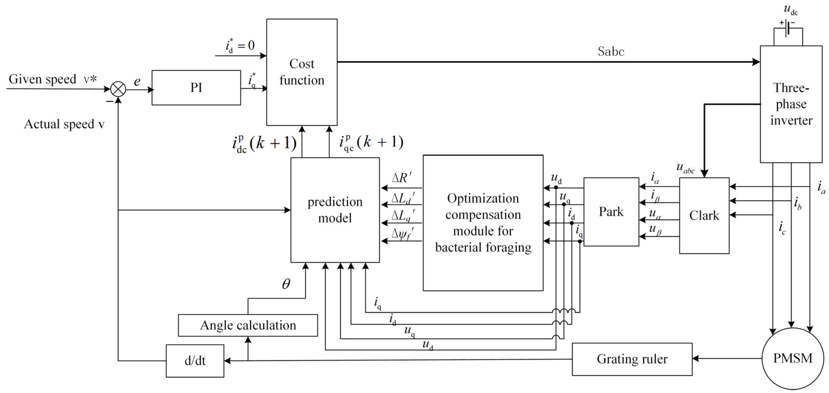
4.2. BFOA Generation Compensation Parameters

Applying BFOA to the generation of compensation parameter Δ R ,   Δ L d ,   Δ L q ,   Δ ψ , the position information of a single bacterium i contains a 4-dimensional vector and can be represented as:
P i = [ Δ R i Δ L d i Δ L q i Δ ψ i ]
Δ R i represents the i-th stator resistance compensation generated, and Δ L d i , Δ L q i , Δ ψ i are the same. To ensure that the compensation parameters meet Equations (35)–(38) and effectively improve the robustness of the control system, the fitness function of bacteria should be set as follows:
J 1 = T L dm ( L dm + Δ L d ) { [ u d ( k ) R m i d ( k ) + L qm ω e ( k ) i q ( k ) ] Δ L d [ L dm ω e ( k ) i q ( k ) ] Δ L q + [ L dm i d ( k ) ] Δ R }
J 2 = T L qm ( L qm + Δ L q ) { [ u q ( k ) R m i q ( k ) L dm ω e ( k ) i d ( k ) ψ fm ω e ( k ) ] Δ L q + [ L qm ω e ( k ) i d ( k ) ] Δ L d + [ L qm i q ( k ) ] Δ R + [ L qm ω e ( k ) ] Δ ψ }
J 3 = u d ( k ) ( R m + Δ R ) i d ( k ) + ( L qm + Δ L q ) ω e ( k ) i q ( k )
J 4 = u q ( k ) ( R m + Δ R ) i q ( k ) ( L dm + Δ L d ) ω e ( k ) i d ( k ) ( ψ fm + Δ ψ ) ω e ( k )
When the fitness functions J 1 , J 2 , J 3 , J 4 of the corresponding position of a certain bacterium i both tend to 0, it indicates that the bacterium is located in a food-dense location, that is, Δ R ' i Δ L d ' i Δ L q ' i Δ ψ i are close to the optimal compensation parameters. When the fitness functions J 1 , J 2 , J 3 , J 4 tend to infinity or not all tend to 0, then the compensation parameters still need to be iteratively optimized. The specific algorithm flowchart for BFOA parameter compensation is shown in Figure 2. In addition, in order to further enhance readers’ understanding of the BFOA algorithm, Appendix A provides MATLAB code examples for optimizing PID parameters using BFOA.

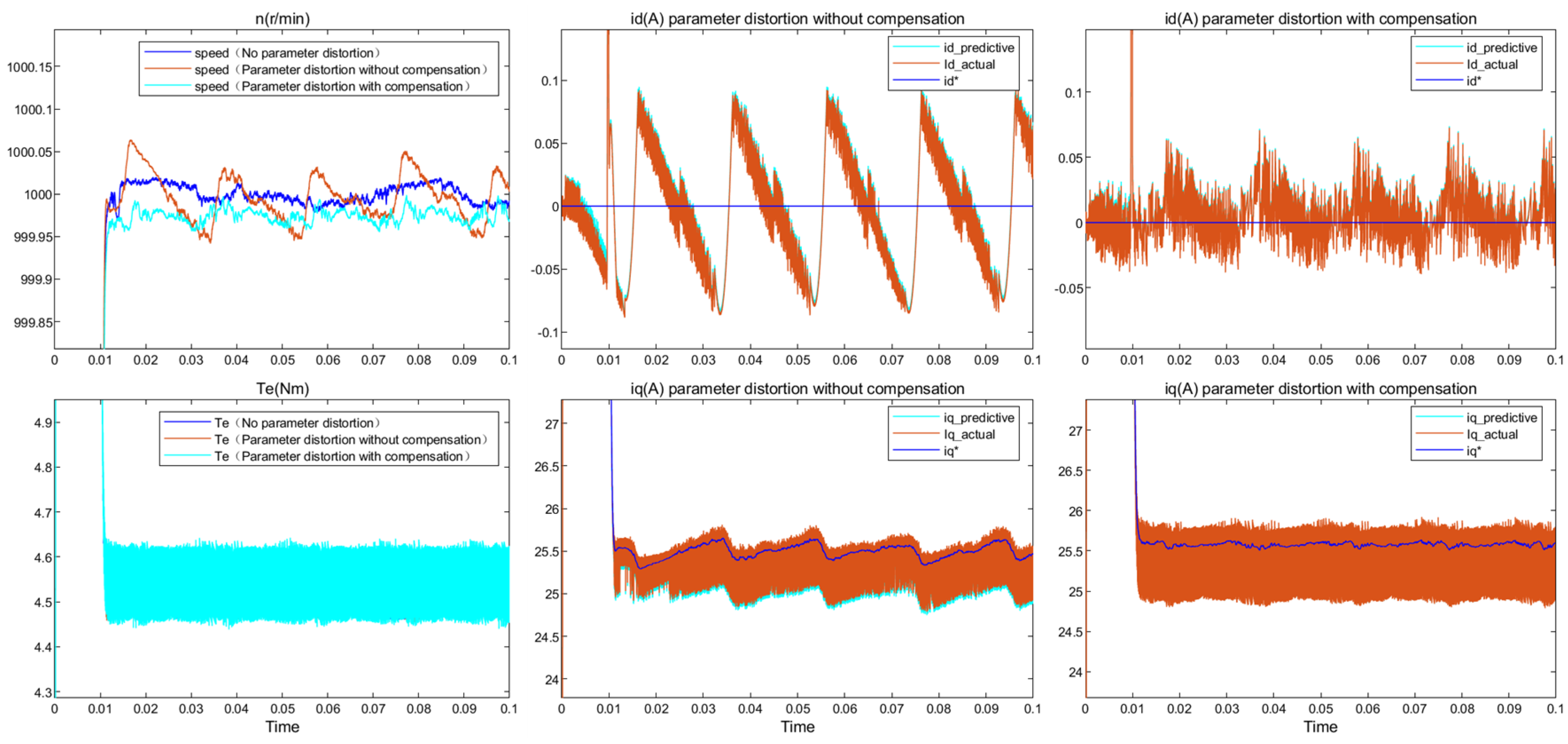
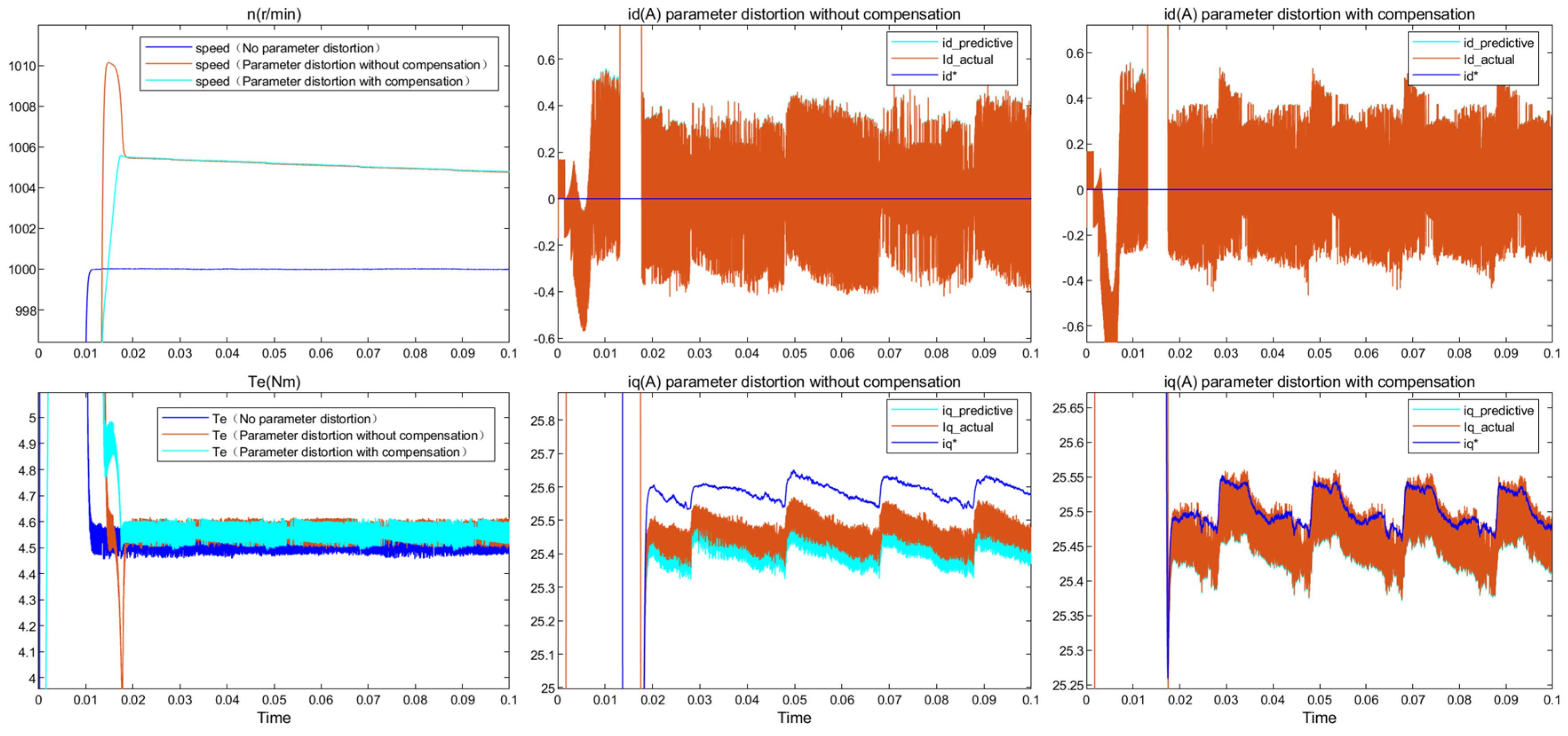
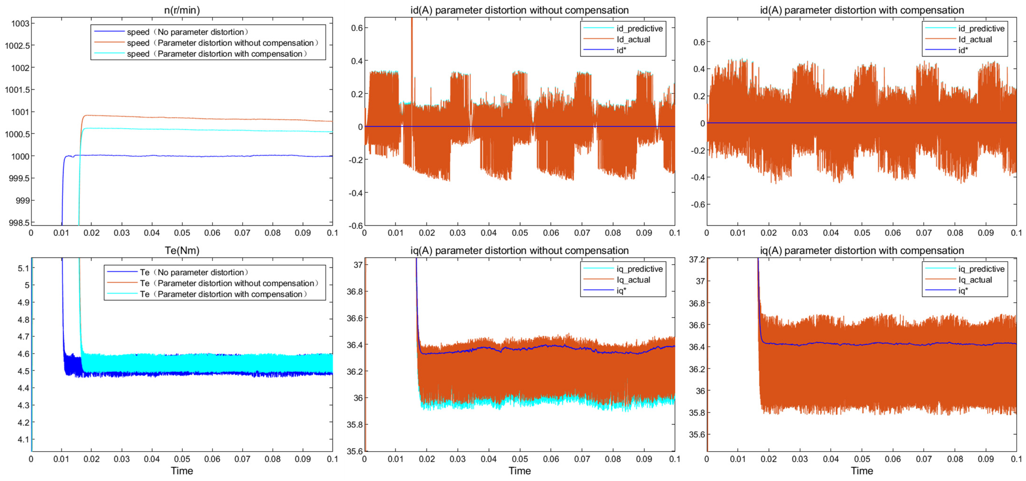
5. Simulation and Verification

In order to verify the correctness and effectiveness of the proposed PMSM predictive control parameter compensation model, a simulation comparison was conducted between the traditional PMSM predictive control model and the predictive control model combined with BFOA using the MATLAB Simulink platform.
The block diagram of the traditional predictive control system is shown in Figure 3. The system adopts a dual closed-loop control structure, with the outer loop being the speed loop, the inner loop being the current loop, and the inverter is a midpoint-clamped three-level inverter. The outer ring performs PI control based on speed feedback to obtain the reference current value of the motor’s q-axis. The inner loop prediction model obtains the predicted current values of the d and q axes based on the motor calibration parameters. The cost function determines the inverter switch state based on the difference between the predicted current and the reference current, thereby achieving tracking for a given speed. When the actual parameters of the motor deviate from the calibration parameters in complex experimental environments, such as high temperatures, BFOA will output parameter compensation based on multiple fitness functions. When the compensation is applied to the prediction model, the cost function will redetermine the inverter switch state to achieve disturbance regulation. The BFOA predictive control system diagram is shown in Figure 4.
Build a comparative simulation experiment according to the block diagram, and the PMSM parameters in the experiment are shown in Table 1. Under the experimental conditions of a given speed of 1000 r/min and a load of 1.27 Nm, five sets of parameter distortion control experiments were set up:
  • R s = 2 R sm ;
  • L d = 2 L dm ;
  • L q = 2 L qm ;
  • ψ f = 0.7 ψ fm ;
  • R s = 1.5 R sm ,   L d = 1.5 L dm ,   L q = 1.5 L qm ,   ψ f = 0.7 ψ fm ;
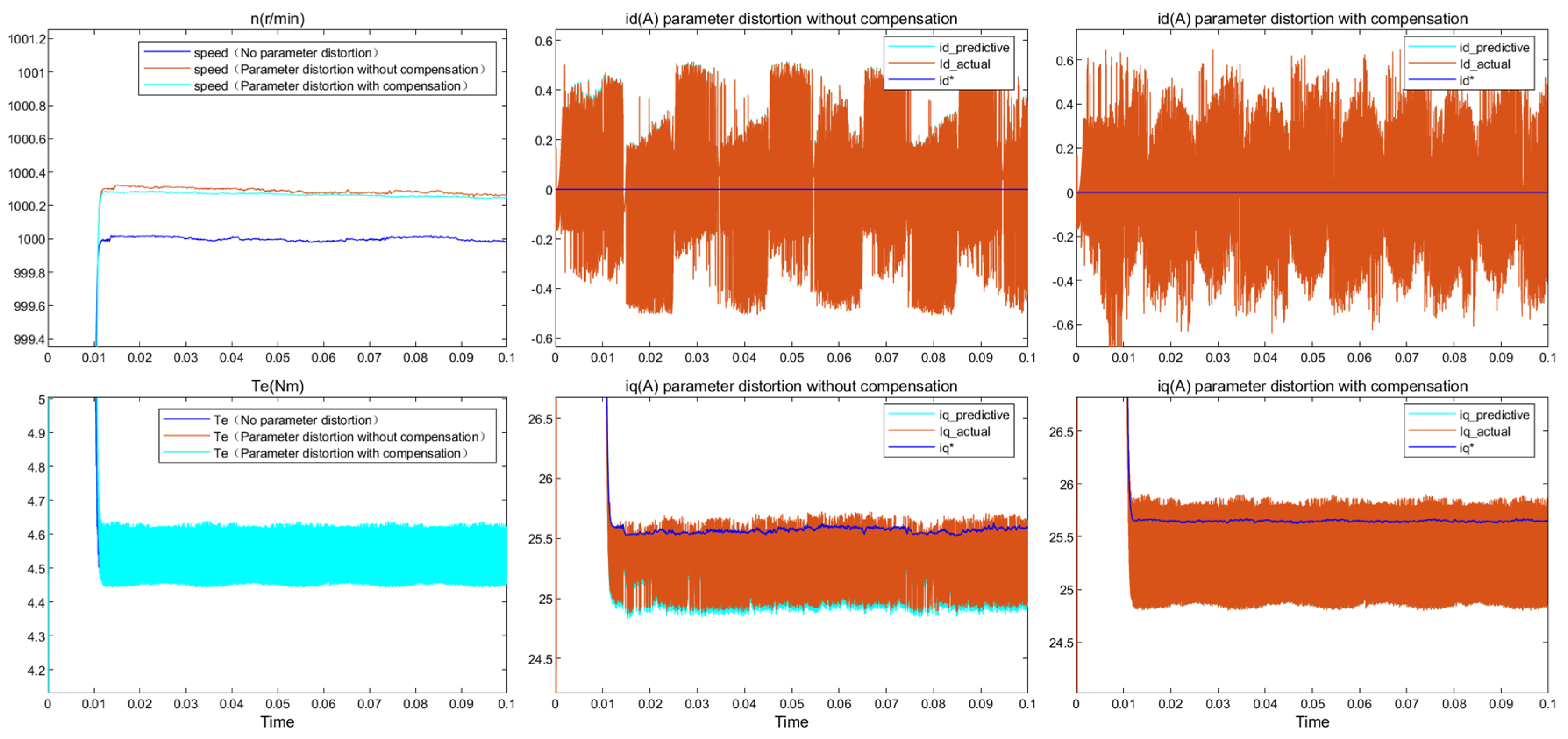
  • Change the calibration parameters in the simulation motor to simulate parameter distortion. The first four sets of experiments will change individual parameters to simulate distortion, and the last set of experiments will cause distortion of all four sets of parameters simultaneously.
The response simulation diagrams for five sets of experiments are shown in Figure 5, Figure 6, Figure 7, Figure 8 and Figure 9, where Figure 5 follows the order of speed response diagram, torque response diagram, d-axis current tracking diagram, and q-axis current tracking diagram from left to right and from top to bottom. The speed response diagram and torque response diagram both include three situations: parameter not distorted, distortion not compensated, and BFOA parameter compensation after distortion. The current tracking chart is divided into two situations: parameter distortion not compensated and parameter distortion compensated, and each chart includes three current tracking situations: reference current, predicted current, and actual current. The situation in Figure 7, Figure 8 and Figure 9 is consistent with Figure 5.
Analysis of simulation results shows that stator resistance distortion can cause steady-state deviation in speed, and the predicted current on the q-axis deviates from the actual current. The distortion of the d-axis inductance will cause pulsation of the speed, obvious pulsation of the d-axis current, and a deviation between the predicted current and the actual current on the q-axis. Distortion of the q-axis inductance can cause an overshoot of the speed, distortion of the q-axis current, and deviation in the actual current tracking predicted current. The distortion of the permanent magnet flux linkage parameter will affect the speed response speed, and there will be a steady-state deviation in the speed, resulting in a deviation between the predicted current of the q-axis and the actual current.
After using BFOA for parameter compensation, all five experiments showed compensation effects. Firstly, the motor speed improved in stability, accuracy, and other aspects, while the overshoot amplitude decreased. Secondly, the fluctuation amplitude of the q-axis current was reduced, making the predicted current more accurate in tracking the actual current, eliminating static bias, and the fluctuation amplitude of the d-axis current was reduced, making it smoother and more stable. The dynamic and static performance of the control system has improved. However, compensation cannot eliminate the influence of parameter distortion, as the newly proposed cost function cannot be completely zero. How to further improve the compensation effect still needs to be studied.
Utilize multiple fitness functions to constrain compensation parameters and achieve real-time compensation.

6. Conclusions

In this article, a parameter compensation scheme for PMSM predictive control based on BFOA is proposed to improve the robustness of the system. The new identification equation effectively solves the problem of insufficient rank in traditional online identification methods without the need to construct additional voltage equations or inject current into the d-axis, greatly simplifying the identification operation process. Meanwhile, the BFOA algorithm is different from other algorithms in that its strong global search ability avoids the problem of getting stuck in local optima during the search process, which ultimately affects the identification results. In addition, the research focuses on built-in PMSM, filling the gap in the lack of intelligent algorithm parameter identification for built-in PMSM.
Build comparative experiments on the Simulink simulation platform and distort the motor parameters in both the PMSM traditional predictive control system and the control system with parameter compensation. The experimental results show that the overshoot amplitude of the compensated system motor speed is reduced, and the stability and accuracy are improved. The amplitude of the q-axis current fluctuation is reduced, and the tracking performance is improved. It has a compensating effect on single and multi-parameter distortions. The safe operation of the high-performance predictive control system for permanent magnet synchronous motors has been achieved.
However, compensation cannot completely eliminate the impact of distortion on performance, and the effect of compensating for resistance distortion is limited. How to further improve the compensation effect still needs to be studied. In addition, the research on compensation performance in high-, medium-, and low-speed fields is the main focus of my further research.

Author Contributions

Conceptualization, Formal analysis, Supervision Y.S. and Y.T.; Investigation, Software validation, Writing and editing, J.Y. All authors have read and agreed to the published version of the manuscript.

Funding

This research received no external funding.

Institutional Review Board Statement

Not applicable.

Informed Consent Statement

Not applicable.

Data Availability Statement

Data is contained within the article. The data presented in this study are available in Appendix A.

Acknowledgments

The author sincerely appreciates the infrastructure provided by the Jiangnan University Internet of Things Engineering College for conducting this research work, as well as the support and academic guidance provided by the supervisor for this published article.

Conflicts of Interest

The authors declare no conflict of interest. Yongqiang Tan is an employee of Nanjing Power Supply Branch of State Grid Jiangsu Electric Power Co., Ltd. The paper reflects the views of the scientists and not the company.

Nomenclature

ParameterValue
u a ,   u b ,   u c Stator three-phase voltages
i a ,   i b ,   i c Stator three-phase currents
ψ a ,   ψ b ,   ψ c Three-phase winding flux linkage
R s Stator resistance
u d ,   u q Direct axis and quadrature axis voltage
i d ,   i q Direct axis and quadrature axis current
ψ d ,   ψ q Direct axis and quadrature axis flux linkage
T Sampling time
*   S w ( : , i ) Eight   states   of   three   sets   of   switches   for   inverters ,   including   ( 000 , 001 , 010 , 011 , 100 , 101 , 110 , 111 ) ,   i = 1 , 2 , 3 , 4 , 5 , 6 , 7 , 8
u dc Inverter DC voltage source
i d ( k ) ,   i q ( k ) Present value of Direct axis and quadrature axis current
i d ( k + 1 ) ,   i q ( k + 1 ) Future value of Direct axis and quadrature axis current
J Cost function/Fitness function
i d r e f ,   i q r e f Reference value of Direct axis and quadrature axis current
i d p ( k + 1 ) ,   i q p ( k + 1 ) Theoretical value of predicted current for d and q axis
R m ,   L dm ,   L qm ,   ψ fm Model values without distortion of motor parameters
i d a ( k + 1 ) ,   i q a ( k + 1 ) Actual value of predicted current for d and q axis
R a , L da , L qa , ψ fa Actual values with distortion of motor parameters
Δ R , Δ L d , Δ L q , Δ ψ Distortion value of corresponding parameters
i dc p ( k + 1 ) , i qc p ( k + 1 ) Predicted current values of d and q axes after compensation
Δ R ,   Δ L d ,   Δ L q ,   Δ ψ Compensation values of corresponding parameters
d e v d 1 , d e v d 2 D-axis predicted the current deviation component
d e v q 1 ,   d e v q 2 Q-axis predicted the current deviation component
*   P i Location information of bacteria i
*   C ( i ) Unit of step length during bacterial swimming
*   Δ ( i ) Randomly generated direction vector
N s Number of swimming steps
N c Chemotaxis frequency
N re Reproduction frequency
N ed Number of dispersion times
J ( j , k , l ) The corresponding goodness of the position information
* The bold font in the table represents the matrix.

Appendix A

MATLAB code examples for optimizing PID parameters using BFOA.
Nc = 50;          % Chemotaxis frequency
Ns = 4;                          % Swimming frequency
Nre = 4;          % Copy count
Ned = 2;         % Disperse (migrate) times
sizepop = 20;       % Population size
Sr = sizepop/2;       % Number of copies (splits)
nvar = 3;         % 3 unknown quantities
Ped = nvar/12;        % Probability of bacterial dispersal (migration)
popmin = [0,0,0];    % x min
popmax = [30,30,30];   % x max
Cmin = [−2,−2,−2];   % Minimum step size
Cmax = [2,2,2];    % Maximum step size
C(:,:) = 0.001*ones(sizepop,nvar);  % After selecting the flipping direction, the step size of a single bacteria moving forward
%% The cost function, which is our objective function
fun = @(x)PID_Fun_1(x);
%% Initialize population
for I = 1:sizepop
  pop(i,:) = popmin + (popmax-popmin).*rand(1,nvar);  % Initialize individual
  fitness(i) = fun( pop(i,:) );      % Initialize fitness value
  C(i,:) = Cmin + (Cmax-Cmin).*rand(1,nvar); % Initialization step size
end
%% Record a set of optimal values
[bestfitness,bestindex] = min(fitness); % Take the minimum fitness value
zbest = pop(bestindex,:);  % Global best bacterial individual
fitnesszbest = bestfitness; % Global optimal fitness value
%% Iterative optimization
for i = 1:Ned         % Disperse (migrate) times
  for k = 1:Nre        % Copy count
     for m = 1:Nc      % Chemotaxis frequency
      for j = 1:sizepop   % population
        % Flip
        delta = 2*rand(1,nvar)-0.5;
        pop(j,:) = pop(j,:) + C(j,:).*delta./(sqrt( delta*delta’ ));
        
        % Value range constraint
        pop(j,:) = 1b_ub(pop(j,:), popmin, popmax);
 
        % Update the current fitness value
        fitness(j) = fun(pop(j,:));
 
        % Fitness update
        % Comparison between bacterial individuals
        if fitness(j) < fitnesszbest
         fitnesszbest = fitness(j);
         zbest = pop(j,:);
        end
      end
    end
    % Copy operation
    [maxF,index] = sort(fitness,‘descend’); % Sort in descending order
    for Nre2 = index:Sr % Update half of the population with higher fitness values
      pop(Nre2,:) = popmin + (popmax-popmin).*rand(1,nvar);
      fitness(Nre2) = fun(pop(Nre2,:));
      C(Nre2,:) = Cmin + (Cmax-Cmin).*rand(1,nvar); % Update step size
      % Comparison between bacterial individuals
      if fitness(Nre2) < fitnesszbest
        fitnesszbest = fitness(Nre2);
        zbest = pop(Nre2,:);
      end
     end
  end
 % Disperse (migrate) operation
 for j = 1:sizepop
     if Ped > rand
      pop(j,:) = popmin + (popmax-popmin).*rand(1,nvar);
      fitness(j) = fun(pop(j,:));
      % Comparison between bacterial individuals
      if fitness(j) < fitnesszbest
        fitnesszbest = fitness(j);
        zbest = pop(j,:);
      end
     end
  end
end

function BsJ = PID_Fun_1(Kpidi)
ts = 0.001;
sys = tf([1.0],[1 1],‘ioDelay’,0.2);
dsys = c2d(sys,ts,‘z’);
[num,den] = tfdata(dsys,‘v’);
u_1 = 0.0;
y_1 = 0.0;
x = [0,0,0]’;
B = 0;
error_1 = 0;
s = 0;
P = 1000;
for k = 1:1:P
  timef(k) = k*ts;
  r(k) = 1;
  u(k) = Kpidi(1)*x(1) + Kpidi(2)*x(3) + Kpidi(3)*x(2);
   if u(k)> = 10
    u(k) = 10;
   end
   if u(k)< = −10
    u(k) = −10;
   end
  yout(k) = -den(2)*y_1 + num(2)*u_1;
  error(k) = r(k)-yout(k);
  %-------------------Return of PID parameters----------------
  u_1 = u(k);
  y_1 = yout(k);
  x(1) = error(k);        % Calculating  P
  x(2) = (error(k)-error_1)/ts;   % Calculating  D
  x(3) = x(3) + error(k)*ts;    % Calculating  I
  error_1 = error(k);
  if s==0
     if yout(k) > 0.95 && yout(k) < 1.05
      tu = timef(k);
      s = 1;
     end
  end
end
 for i = 1:1:P
   Ji(i) = 0.999*abs(error(i)) + 0.01*u(i)^2*0.1;
   B = B+Ji(i);
   if i > 1
    erry(i) = yout(i)-yout(i-1);
    if erry(i) < 0
       B = B + 100*abs(erry(i));
    end
   end
 end
 BsJ = sum(abs(error));
 end

References

  1. Development and Reform Commission Energy Bureau. The 14th Five Year Plan for Modern Energy System [Z]. The Central People’s Government of the People’s Republic of China Website. Available online: https://www.gov.cn/zhengce/zhengceku/2022-03/23/content_5680759.htm (accessed on 29 January 2022).
  2. CRRC Yunshang Information Technology Co., Ltd.; Guangdong Lingtai Education Resources Co., Ltd. New Energy Vehicle Drive Motor Technology; Mechanical Industry Press: Beijing, China, 2023. [Google Scholar]
  3. Xiao, Z.; Hu, M.; Shi, L.; Zhou, A. Online estimation of rotor temperature for built-in permanent magnet synchronous motors in electric vehicles. J. Mech. Eng. 2023, 11, 1–14. [Google Scholar]
  4. Xie, Y.; Sun, C.; Cai, W.; Ren, S.; Sun, C. Study on the loss of excitation mechanism and selected area heavy rare earth infiltration of permanent magnet synchronous motors for electric vehicles. J. Electr. Mach. Control. 2023, 5, 1–9. [Google Scholar]
  5. Xie, Y.; He, P.; Cai, W.; Liu, H. Design and optimization of permanent magnet synchronous motors with hairpin winding for vehicles. J. Electr. Mach. Control. 2021, 25, 36–45. [Google Scholar]
  6. Qi, X.; Su, T.; Zhou, K.; Yang, J.; Gan, X.; Zhang, Y. Overview of the Development of Model Predictive Control Strategies for AC Motors. Chin. J. Electr. Eng. 2021, 41, 6408–6419. [Google Scholar]
  7. Rodriguez, J.; Cristian, G.; Andres, M.; Freddy, F.-B.; Pablo, A.; Mateja, N.; Yongchang, Z.; Luca, T.; Alireza, D.; Zhenbin, Z. Latest advances of model predictive control in electrical drives—Part I: Basic concepts and advanced Strategies. IEEE Trans. Power Electron. 2022, 37, 3927–3942. [Google Scholar] [CrossRef]
  8. Yao, X.; Huang, C.; Wang, J.; Ma, H.; Liu, T.; Zhang, G. Dual vector model predictive current control for permanent magnet synchronous motors with parameter identification function. Chin. J. Electr. Eng. 2022, 10, 1–13. [Google Scholar]
  9. Peng, J.; Yao, M. Overview of Predictive Control Technology for Permanent Magnet Synchronous Motor Systems. Appl. Sci. 2023, 13, 6255. [Google Scholar] [CrossRef]
  10. Wang, L.; Zhao, J.; Yang, X.; Zheng, Z.; Zhang, X.; Wang, L. Robust Deadbeat Predictive Current Regulation for Permanent Magnet Synchronous Linear Motor Drivers with Parallel Parameter Disturbance and Load Observer. IEEE Trans. Power Electron. 2022, 37, 7834–7845. [Google Scholar] [CrossRef]
  11. Sun, X.; Zhang, Y.; Lei, G.; Guo, Y.; Zhu, J. An improved deadbeat predictive stator flux control with reduced-order disturbance observer for in-wheel PMSMs. IEEE/ASME Trans. Mechatron. 2021, 27, 690–700. [Google Scholar] [CrossRef]
  12. Li, Z.; Feng, G.; Lai, C.; Banerjee, D.; Li, W.; Kar, N.C. Current injection-based multi-parameter estimation for dual three-phase IPMSM considering VSI nonlinearity. IEEE Trans. Transp. Electrif. 2019, 5, 405–415. [Google Scholar] [CrossRef]
  13. Li, X.; Kennel, R. General formulation of kalman-filter-based online parameter identification methods for VSI-Fed PMSM. IEEE Trans. Ind. Electron. 2021, 68, 2856–2864. [Google Scholar] [CrossRef]
  14. An, X.; Liu, G.; Chen, Q.; Zhao, W.; Song, X. Adjustable model predictive control for IPMSM drives based on online stator inductance identification. IEEE Trans. Ind. Electron. 2022, 69, 3368–3381. [Google Scholar] [CrossRef]
  15. Boileau, T.; Leboeuf, N.; Nahid-Mobarakeh, B.; Meibody-Tabar, F. Online identification of PMSM parameters: Parameter identify-ability and estimator comparative study. IEEE Trans. Ind. Appl. 2011, 47, 1944–1957. [Google Scholar] [CrossRef]
  16. Zhou, M.; Jiang, L.; Wang, C. Real-Time Multiparameter Identification of a Salient-Pole PMSM Based on Two Steady States. Energies 2020, 13, 6109. [Google Scholar] [CrossRef]
  17. Yu, Y.; Huang, X.; Li, Z.; Wu, M.; Shi, T.; Cao, Y.; Yang, G.; Niu, F. Full Parameter Estimation for Permanent Magnet Synchronous Motors. IEEE Trans. Ind. Electron. 2022, 69, 4376–4386. [Google Scholar] [CrossRef]
  18. Zhang, Y.G.; Yin, Z.G.; Sun, X.D.; Zhong, Y.R. On-line identification methods of parameters for permanent magnet synchronous motors based on cascade MRAS. In Proceedings of the 2015 9th International Conference on Power Electronics and ECCE Asia (ICPE 2015-ECCE Asia), Seoul, Republic of Korea, 1–5 June 2015. [Google Scholar]
  19. Feng, G.; Lai, C.; Mukherjee, K.; Kar, N.C. Current Injection-Based Online Parameter and VSI Nonlinearity Estimation for PMSM Drives Using Current and Voltage DC Components. IEEE Trans. Transp. Electrif 2016, 2, 119–128. [Google Scholar] [CrossRef]
  20. Liu, Z.; Wei, H.; Zhong, Q.; Liu, K.; Li, X.H. GPU implementation of DPSO-RE algorithm for parameters identification of surface PMSM considering VSI nonlinearity. Emerging Sel. Top. Power Electron 2017, 5, 1334–1345. [Google Scholar] [CrossRef]
  21. Liu, Z.H.; Zhang, J.; Zhou, S.W.; Li, X.H.; Liu, K. Coevolutionary particle swarm optimization using AIS and its application in multiparameter estimation of PMSM. IEEE Trans. Cybern 2013, 43, 1921–1935. [Google Scholar] [CrossRef]
  22. Liu, L.; Liu, W.X.; Cartes, D.A. Permanent magnet synchronous motor parameter identification using particle swarm optimization. Comput. Intell. Res. 2008, 4, 211–218. [Google Scholar] [CrossRef]
  23. Kou, P.; Zhou, J.; Li, C.; He, Y.; He, H. Identification of hydraulic turbine governor system parameters based on Bacterial Foraging Optimization Algorithm. In Proceedings of the 2010 Sixth International Conference on Natural Computation, Yantai, China, 10–12 August 2010; pp. 3339–3343. [Google Scholar]
  24. Niu, B.; Liu, J.; Wu, T.; Chu, X.; Wang, Z.; Liu, Y. Coevolutionary Structure-Redesigned-Based Bacterial Foraging Optimization. IEEE/ACM Trans. Comput. Biol. Bioinform. 2018, 15, 1865–1876. [Google Scholar] [CrossRef]
  25. Wang, D.; Qian, X.; Ban, X.; Ma, B.; Ma, Y.; Lv, Z. Enhanced Bacterial Foraging Optimization Based on Progressive Exploitation Toward Local Optimum and Adaptive Raid. IEEE Access 2019, 7, 95725–95738. [Google Scholar] [CrossRef]
  26. Holtz, J.; Stadtfeld, S. A predictive controller for the stator current vector of AC machines fed from a switched voltage source. In Proceedings of the International Power Electronics Conference (IPEC), Tokyo, Japan, 27–31 March 1983; pp. 1665–1675. [Google Scholar]
  27. Tang, J.; Liu, G.; Pan, Q. A Review on Representative Swarm Intelligence Algorithms for Solving Optimization Problems: Applications and Trends. IEEE/CAA J. Autom. Sin. 2021, 8, 1627–1643. [Google Scholar] [CrossRef]
  28. Dong, H.K.; Cho, C.H. Bacteria Foraging Based Neural Network Fuzzy Learning. In Proceedings of the 2nd Indian International Conference on Artificial Intelligence, Pune, India, 20–22 December 2005. [Google Scholar]
  29. Kim, D.H.; Abraham, A.; Cho, J.H. A hybrid genetic algorithm and bacterial foraging approach for global optimization. Inf. Sci. 2007, 177, 3918–3937. [Google Scholar] [CrossRef]
  30. Chen, D.; Zhang, G.; Yao, C.; Zhang, R. Optimization algorithm for bacterial foraging and application of PID parameter optimization. China Mech. Eng. 2014, 25, 59–64. [Google Scholar] [CrossRef]
Figure 1. Schematic diagram of a three-phase bridge inverter circuit.
Wevj 15 00023 g001
Figure 2. Flow chart of BFOA parameter compensation.
Wevj 15 00023 g002
Figure 3. Traditional FCS-MPCC control block diagram.
Wevj 15 00023 g003
Figure 4. BFOA predictive control system block diagram.
Wevj 15 00023 g004
Figure 5. System simulation response diagram of R distortion.
Wevj 15 00023 g005
Figure 6. System simulation response diagram of Ld distortion.
Wevj 15 00023 g006
Figure 7. System simulation response diagram of Lq distortion.
Wevj 15 00023 g007
Figure 8. System simulation response diagram of ψ f distortion.
Wevj 15 00023 g008
Figure 9. System simulation response diagram of multiparameter distortion.
Wevj 15 00023 g009
Table 1. PMSM simulation parameters.
ParameterValue
Stator resistance R / Ω 0.0485
D-axis inductance L d / H 0.000395
Q-axis inductance L q / H 0.000395
Permanent magnet flux chain ψ f / Wb 0.1194
Rotational inertia J / kg m 2 0.0027
DC voltage source U dc / V 220
Load torque T r / Nm 1.27
Given speed r / min 1000
Population size N 5000
Swimming steps N s 25
Chemotaxis frequency N c 50
Reproduction frequency N r e 2
Migration probability P e d 0.25
Dispersion frequency N e d 2
Disclaimer/Publisher’s Note: The statements, opinions and data contained in all publications are solely those of the individual author(s) and contributor(s) and not of MDPI and/or the editor(s). MDPI and/or the editor(s) disclaim responsibility for any injury to people or property resulting from any ideas, methods, instructions or products referred to in the content.

