
Electric Vehicle and Photovoltaic Power Scenario Generation under Extreme High-Temperature Weather

Abstract
1. Introduction
2. Kernel Density Estimation and Model Testing Methods
2.1. Kernel Density Estimation Method
2.2. Model-Checking Method
2.2.1. Goodness of Fit Test
- (1)
- Pearson
- (2)
- Kolmogorov–Smirnov
2.2.2. Test of Fitting Accuracy
3. Correlation Modeling and Scene Generation of PV and EV Power under High-Temperature Weather Based on Copula Theory
3.1. Copula-Related Theory
3.1.1. Copula Functions and Classification
3.1.2. PV Systems and EV Modeling
- (1)
- PV Modeling
- (2)
- EV Modeling
3.1.3. Optimal Choice of Copula Function
- (1)
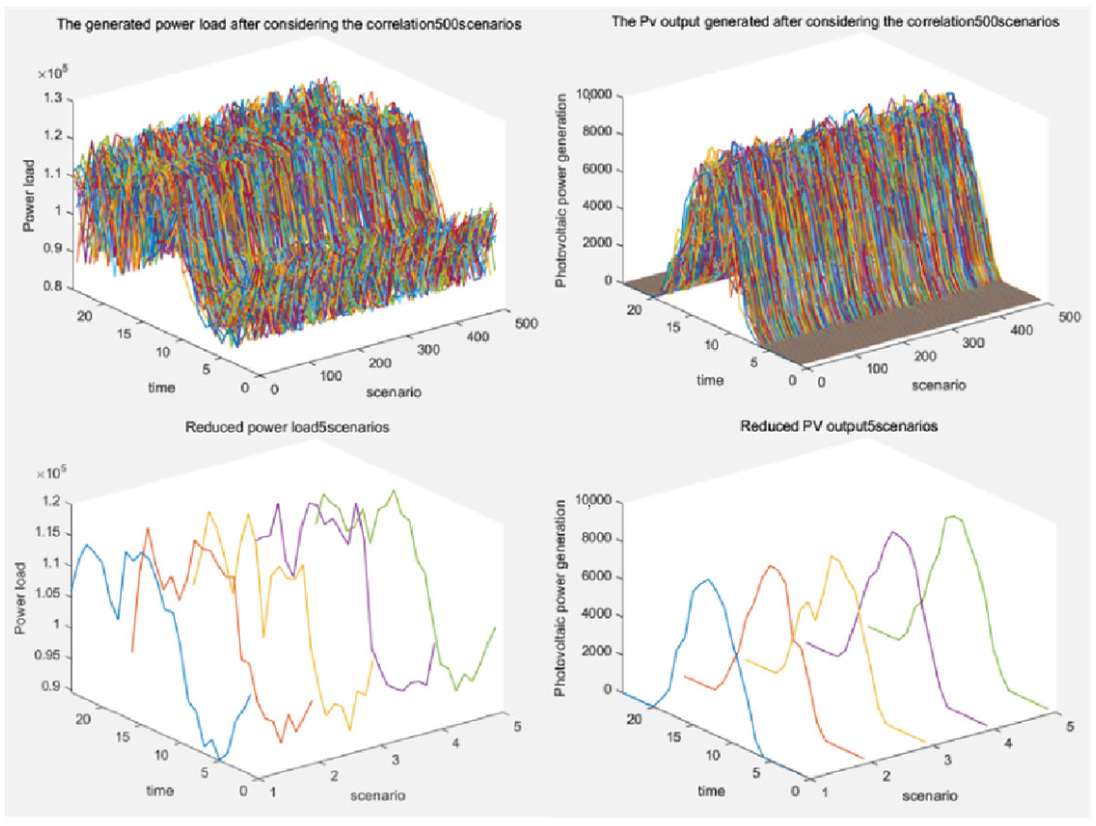
- Joint scenario generation and reduction of PV and EV power
- ①
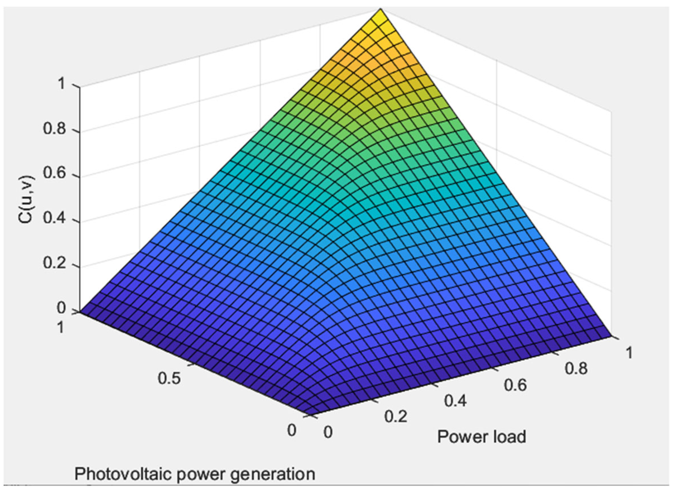
- Functional image discrimination is to compare the probability density function images of each copula function with the probability density function of the sample data, and the closest image is the optimal copula function.
- ②
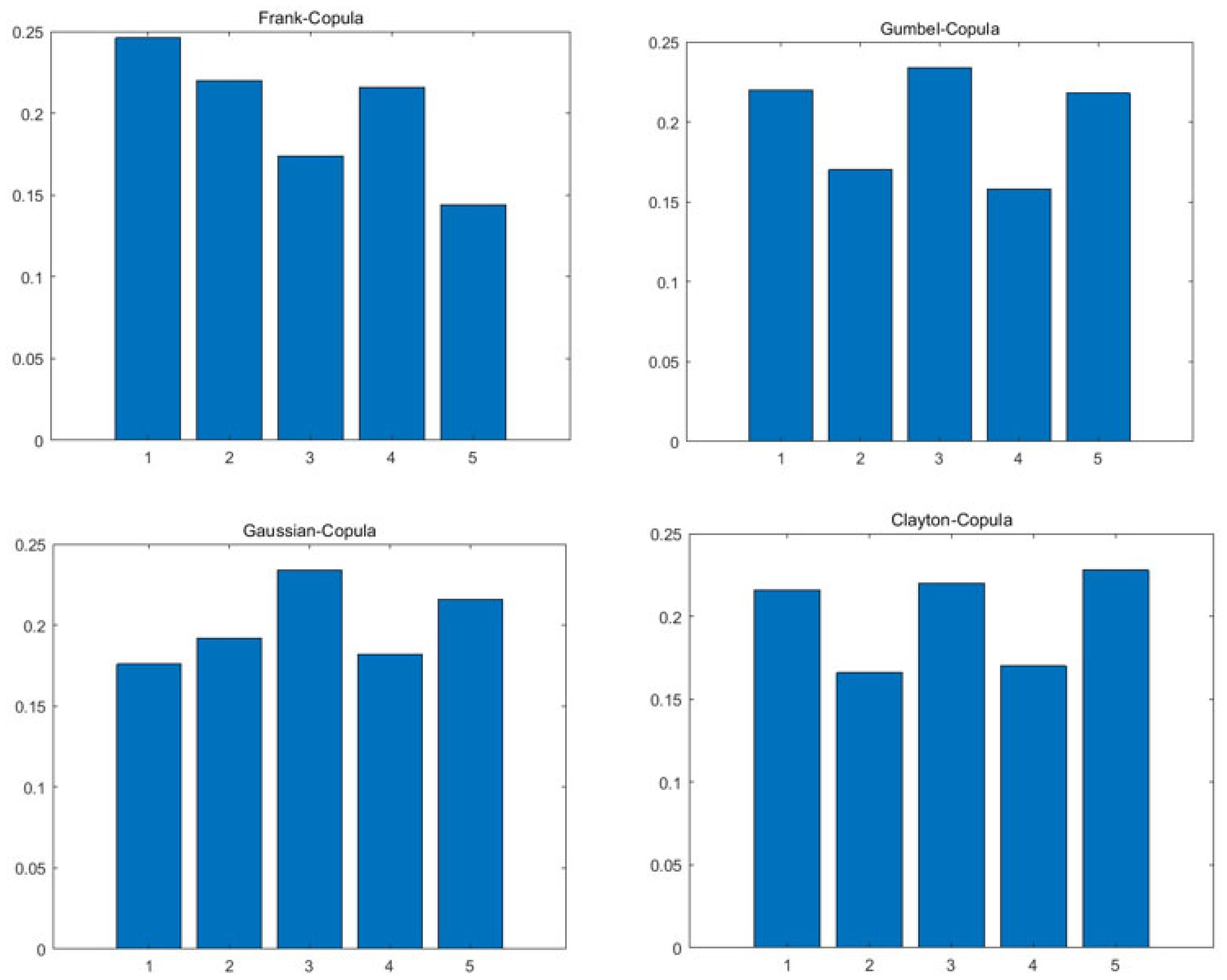
- Correlation coefficient discrimination method is to judge the goodness of fit using the Kendall rank correlation coefficient and Spearman rank correlation coefficient. The rank correlation coefficients of various copula functions are compared with the rank correlation coefficients of sample data. The closer the data are, the better the goodness of fit is, and the corresponding copula function is the best.
- ③
- The Euclidean distance discrimination method is to compare the Euclidean distance of each copula function with the empirical copula function of the sample data. The smaller the Euclidean distance is, the better the goodness of fit of the copula function is.
- (2)
- Scenario generation based on cubic spline interpolation
- (3)
- Scenario reduction based on k-means clustering algorithm
4. Case Study
5. Conclusions
Author Contributions
Funding
Institutional Review Board Statement
Informed Consent Statement
Data Availability Statement
Conflicts of Interest
Appendix A

| Description | |
|---|---|
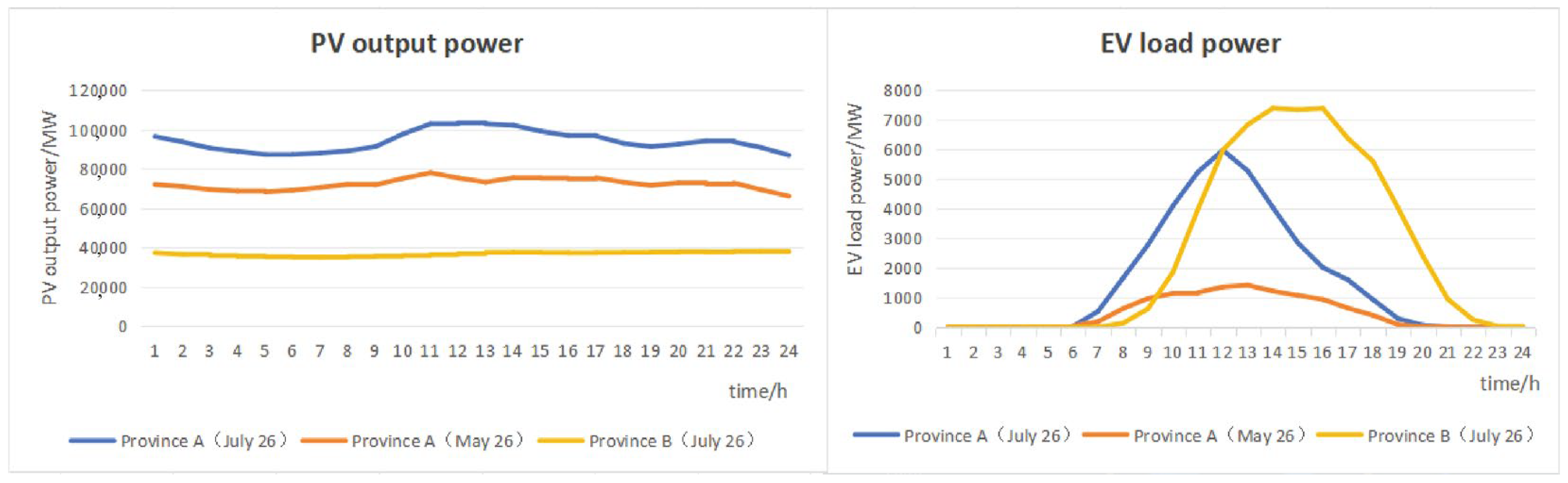
| Diurnal Variation Curve | The diurnal variation curve of a photovoltaic power station illustrates the change in power generation over the course of a day. Typically, power generation gradually increases at sunrise, may reach its peak around noon, and then gradually decreases until sunset. |
| Seasonal Variation | The power generation of a photovoltaic power station is influenced by seasonal changes. Summer, with longer sunlight hours and a higher solar zenith angle, may result in higher peak power during this season. |
| Weather Impact | Weather conditions, such as clear, cloudy, or overcast skies, directly affect the output of a photovoltaic power station. Cloudy weather can lead to fluctuations and a reduction in power generation. |
| Shadow Effect | If the photovoltaic power station is affected by shadows from buildings, trees, or other objects, irregular fluctuations may appear on the curve, known as the shadow effect. |
| Start and End Times | The times when a photovoltaic power station begins and ends its power generation, influenced by sunrise and sunset times. |
| Peak Power | The highest power generation of the photovoltaic power station during the day, typically occurring at noon when the solar zenith angle is at its maximum. |
| Power Fluctuations | The fluctuation in power on the power curve of the photovoltaic power station, representing instantaneous changes in power, potentially influenced by shadows, cloud cover, and other weather factors. |
| Description | |
|---|---|
| Charging Peak Period | Electric vehicles may experience a charging peak at night or during specific time periods, indicating users’ tendency to charge during low electricity price periods. |
| Driving Peak Period | Daytime may witness a driving peak, signifying higher usage demand for electric vehicles during the day. |
| Charging Efficiency Variations | The charging curve may reflect variations in charging efficiency at different charging power levels, influenced by battery and charging equipment performance. |
| Charging Time Distribution | Describes the distribution of time required for electric vehicle charging, including short “top-up” charges and longer “full-charge” durations. |
| Load Fluctuations: | Reflects the variability in electric vehicle power demand, with certain periods exhibiting significant power fluctuations. |
| Charging Behavior Response | Describes whether electric vehicles respond to power system demand signals or price signals, adjusting their charging behavior accordingly. |
| Usage Patterns | Distinguishes between weekdays and weekends, as well as different usage patterns during daytime and nighttime. |
References
- Tan, J.; Wu, Q.; Hu, Q.; Wei, W.; Liu, F. Adaptive robust energy and reserve co-optimization of integrated electricity and heating system considering wind uncertainty. Appl. Energy 2020, 260, 114230. [Google Scholar] [CrossRef]
- Zhang, F.; Bieber, L.; Zhang, Y.; Li, W.; Wang, L. A Multi-port DC Power Flow Controller Integrated with MMC Stations for Offshore Meshed Multi-terminal HVDC Grids. IEEE Trans. Sustain. Energy 2023, 14, 1676–1691. [Google Scholar] [CrossRef]
- Yan, J.; Liu, Y.; Han, S.; Wang, Y.; Feng, S. Reviews on uncertainty analysis of wind power forecasting. Renew. Sustain. Energy Rev. 2015, 52, 1322–1330. [Google Scholar] [CrossRef]
- Lee, D.; Baldick, R. Load and wind power scenario generation through the generalized dynamic factor model. IEEE Trans. Power Syst. 2016, 32, 400–410. [Google Scholar] [CrossRef]
- Ahmad, N.; Ghadi, Y.; Adnan, M.; Ali, M. Load forecasting techniques for power system: Research challenges and survey. IEEE Access 2022, 10, 71054–71090. [Google Scholar] [CrossRef]
- Hu, Q.; Li, F.; Fang, X.; Bai, L. A framework of residential demand aggregation with financial incentives. IEEE Trans. Smart Grid 2016, 9, 497–505. [Google Scholar] [CrossRef]
- Dong, X.; Deng, S.; Wang, D. A short-term power load forecasting method based on k-means and SVM. J. Ambient. Intell. Humaniz. Comput. 2022, 13, 5253–5267. [Google Scholar] [CrossRef]
- Fang, X.; Hu, Q.; Li, F.; Wang, B.; Li, Y. Coupon-based demand response considering wind power uncertainty: A strategic bidding model for load serving entities. IEEE Trans. Power Syst. 2015, 31, 1025–1037. [Google Scholar] [CrossRef]
- Hu, Q.; Li, F. Hardware design of smart home energy management system with dynamic price response. IEEE Trans. Smart Grid 2013, 4, 1878–1887. [Google Scholar] [CrossRef]
- Chen, P.; Pedersen, T.; Bak-Jensen, B.; Chen, Z. ARIMA-based time series model of stochastic wind power generation. IEEE Trans. Power Syst. 2009, 25, 667–676. [Google Scholar] [CrossRef]
- Zhang, Y.; Ai, Q.; Xiao, F.; Hao, R.; Lu, T. Typical wind power scenario generation for multiple wind farms using conditional improved Wasserstein generative adversarial network. Int. J. Electr. Power Energy Syst. 2020, 114, 105388. [Google Scholar] [CrossRef]
- Qiu, Y.; Li, Q.; Pan, Y.; Yang, H.; Chen, W. A scenario generation method based on the mixture vine copula and its application in the power system with wind/hydrogen production. Int. J. Hydrogen Energy 2019, 44, 5162–5170. [Google Scholar] [CrossRef]
- Zhang, Y.; Qian, W.; Ye, Y.; Li, Y.; Tang, Y.; Long, Y.; Duan, M. A novel non-intrusive load monitoring method based on ResNet-seq2seq networks for energy disaggregation of distributed energy resources integrated with residential houses. Appl. Energy 2023, 349, 121703. [Google Scholar] [CrossRef]
- Arik, I.; Kantar, Y.M.; Usta, I. The new odd-Burr Rayleigh distribution for wind speed characterization. Wind Struct. 2019, 28, 369–380. [Google Scholar]
- Zhang, W.; Xu, Y. Distributed optimal control for multiple microgrids in a distribution network. IEEE Trans. Smart Grid 2019, 10, 3765–3779. [Google Scholar] [CrossRef]
- Goh, H.H.; Peng, G.; Zhang, D.; Dai, W.; Kurniawan, T.A.; Goh, K.C.; Cham, C.L. A new wind speed scenario generation method based on principal component and R-Vine copula theories. Energies 2022, 15, 2698. [Google Scholar] [CrossRef]
- Zhang, Y.; Shotorbani, A.M.; Wang, L.; Li, W. A Combined Hierarchical and Autonomous DC Grid Control for Proportional Power Sharing with Minimized Voltage Variation and Transmission Loss. IEEE Trans. Power Deliv. 2021, 37, 3213–3224. [Google Scholar] [CrossRef]
- Zhang, S.; Yang, Q.; Gao, Y.; Gao, D. Real-time fire detection method for electric vehicle charging stations based on machine vision. World Electr. Veh. J. 2022, 13, 23. [Google Scholar] [CrossRef]
- Lu, S.; Feng, X.; Lin, G.; Wang, J.; Xu, Q. Non-Intrusive Load Monitoring and Controllability Evaluation of Electric Vehicle Charging Stations Based on K-Means Clustering Optimization Deep Learning. World Electr. Veh. J. 2022, 13, 198. [Google Scholar] [CrossRef]
- Li, H.; Gao, L.; Cai, X.; Zheng, T. Personalized Collision Avoidance Control for Intelligent Vehicles Based on Driving Characteristics. World Electr. Veh. J. 2023, 14, 158. [Google Scholar] [CrossRef]
- Sun, M.; Feng, C.; Zhang, J. Probabilistic solar power forecasting based on weather scenario generation. Appl. Energy 2020, 266, 114823. [Google Scholar] [CrossRef]
- Rocchetta, R.; Li, Y.; Zio, E. Risk assessment and risk-cost optimization of distributed power generation systems considering extreme weather conditions. Reliab. Eng. Syst. Saf. 2015, 136, 47–61. [Google Scholar] [CrossRef]
- Trakas, D.N.; Hatziargyriou, N.D. Resilience constrained day-ahead unit commitment under extreme weather events. IEEE Trans. Power Syst. 2019, 35, 1242–1253. [Google Scholar] [CrossRef]
- Ma, S.; Su, L.; Wang, Z.; Qiu, F.; Guo, G. Resilience enhancement of distribution grids against extreme weather events. IEEE Trans. Power Syst. 2018, 33, 4842–4853. [Google Scholar] [CrossRef]
- Poudyal, A.; Poudel, S.; Dubey, A. Risk-based active distribution system planning for resilience against extreme weather events. IEEE Trans. Sustain. Energy 2022, 14, 1178–1192. [Google Scholar] [CrossRef]

| Name | Formula |
|---|---|
| Box (or uniform) | |
| Cosinus | |
| Epanechnikov | |
| Gaussian | |
| Quaritic | |
| Triangle | |
| Triweight |
| Kendall Rank Correlation Coefficient | Spearman Rank Correlation Coefficient | Square Euclidean Distance | |
|---|---|---|---|
| Gaussian Copula | −0.06664 | −0.09983 | 0.45874 |
| Gumbel Copula | 1.35753 × 10⁻⁶ | 2.05096 × 10⁻⁶ | 2.06240 |
| Clayton Copula | 7.25427 × 10⁻⁷ | 1.09220 × 10⁻⁶ | 2.06237 |
| Frank Copula | −0.09334 | −0.13967 | 0.24974 |
| Sample Data | −0.08268 | −0.12254 | 0 |
Disclaimer/Publisher’s Note: The statements, opinions and data contained in all publications are solely those of the individual author(s) and contributor(s) and not of MDPI and/or the editor(s). MDPI and/or the editor(s) disclaim responsibility for any injury to people or property resulting from any ideas, methods, instructions or products referred to in the content. |
© 2024 by the authors. Licensee MDPI, Basel, Switzerland. This article is an open access article distributed under the terms and conditions of the Creative Commons Attribution (CC BY) license (https://creativecommons.org/licenses/by/4.0/).
Share and Cite
Li, X.; Li, C.; Jia, C. Electric Vehicle and Photovoltaic Power Scenario Generation under Extreme High-Temperature Weather. World Electr. Veh. J. 2024, 15, 11. https://doi.org/10.3390/wevj15010011
Li X, Li C, Jia C. Electric Vehicle and Photovoltaic Power Scenario Generation under Extreme High-Temperature Weather. World Electric Vehicle Journal. 2024; 15(1):11. https://doi.org/10.3390/wevj15010011
Chicago/Turabian StyleLi, Xiaofei, Chi Li, and Chen Jia. 2024. "Electric Vehicle and Photovoltaic Power Scenario Generation under Extreme High-Temperature Weather" World Electric Vehicle Journal 15, no. 1: 11. https://doi.org/10.3390/wevj15010011
APA StyleLi, X., Li, C., & Jia, C. (2024). Electric Vehicle and Photovoltaic Power Scenario Generation under Extreme High-Temperature Weather. World Electric Vehicle Journal, 15(1), 11. https://doi.org/10.3390/wevj15010011