Gradient-Based Metrics for the Evaluation of Image Defogging

Abstract

Fog, haze, or smoke are standard atmospheric phenomena that dramatically compromise the overall visibility of any scene, critically affecting features such as the illumination, contrast, and contour detection of objects. The decrease in visibility compromises the performance of computer vision algorithms such as pattern recognition and segmentation, some of which are very relevant to decision-making in the field of autonomous vehicles. Several dehazing methods have been proposed that either need to estimate fog parameters through physical models or are statistically based. But physical parameters greatly depend on the scene conditions, and statistically based methods require large datasets of natural foggy images together with the original images without fog, i.e., the ground truth, for evaluation. Obtaining proper fog-less ground truth images for pixel-to-pixel evaluation is costly and time-consuming, and this fact hinders progress in the field. This paper aims to tackle this issue by proposing gradient-based metrics for image defogging evaluation that do not require a ground truth image without fog or a physical model. A comparison of the proposed metrics with metrics already used in the NTIRE 2018 defogging challenge as well as several state-of-the-art defogging evaluation metrics is performed to prove its effectiveness in a general situation, showing comparable results to conventional metrics and an improvement in the no-reference scene. A Matlab implementation of the proposed metrics has been developed and it is open-sourced in a public GitHub repository.

1. Introduction

In recent years, there have been important advances in automated surveillance and autonomous vehicles of different kinds. Autonomous vehicles are equipped with sensors, cameras, and advanced software algorithms enabling navigation, decision making, and operation without human intervention. These vehicles are crucial for various reasons, primarily due to their potential to revolutionize transportation by enhancing safety, reducing traffic congestion, and improving energy efficiency. Autonomous vehicles have the capacity to significantly decrease the number of accidents caused by human error provide mobility options for individuals with disabilities or those unable to drive, and optimize transportation systems, thereby mitigating environmental impacts and increasing overall efficiency in our increasingly urbanized world [1].

Nevertheless, image-processing algorithms involved in decision-making for autonomous vehicles perform poorly under adverse weather conditions such as fog, smoke, or haze, since they compromise the image visibility. Other atmospheric scattering media, such as sand or smog, behave similarly. They critically affect the illumination, color, contrast, and contours of the scene due to the scattering behavior of the media.

Therefore, there is a need to achieve a processing solution that reduces the effect of bad weather conditions for image sensors. The process of developing image processing algorithms for enhancing the visibility of images in bad weather conditions is known as defogging or dehazing.

Nowadays, there are several approaches that can be used to defog an image. Firstly, active approaches rely on using gated images [2] or polarized light [3,4] to obtain more information about the scene. Gated imaging usually requires expensive electronics, and polarimetric imaging is challenging to implement in outdoor systems, which is the main target of defogging. Polarimetric images are also complex to automatize and implement in autonomous systems because they usually require an estimation of the physical parameters of the scene [5].

Another common approach to tackle defogging is to apply Deep Neural Networks (DNNs), which have already produced some very promising results. The New Trends in Image Restoration and Enhancement Workshop and Challenges (NTIRE) reflect the advancement in the image defogging field in image and video processing. This workshop proposes challenges in image and video processing in several fields. For instance, homogeneous [6,7] and non-homogeneous [8,9] fog removal were among the topics of interest explored for several years in the workshop. In these challenges, some research groups exploited previous information on the image and tried to evaluate the natural parameters through deep learning techniques [10,11]. Alternatively, other groups took advantage of the generative capability of DNNs, especially with Generative Adversarial Networks (GANs), and used them to directly generate a defogged image from a foggy one without estimating any physical parameters [12,13,14]. In order to evaluate the effectiveness of the defogging networks, classical computer vision metrics such as the structural similarity index (SSIM), the Peak Signal-to-Noise Ratio (PSNR), or CIEDE2000 [15] were used to compare the defogged image with the ground truth of the scene. Nevertheless, classical computer vision metrics for evaluation perform poorly when it comes to quantifying an enhancement in the visibility of the scene. Moreover, and as its most important drawback, these metrics need a defogged ground truth image which is not always available.

Obtaining ground truth images in adverse weather conditions is costly, time-consuming, and, often, simply unfeasible. In natural conditions, fog is a time-variant and complex weather phenomenon. Reproducing the same scene to acquire images without fog but with equivalent luminance, positioning of the objects, etc., is a very complex task in practice. Thus, research is often based on artificial fog generation in rather controlled environments, usually large-scale fog chambers or using smoke-generating machines [16]. However, such artificially generated fog is not fully comparable to natural fog in terms of homogeneity and distribution [17]. This problem is especially sensitive with DNNs because they need huge datasets to achieve good results and avoid overfitting. Even though there are defogging DNNs that are trained in an unpaired manner [12], the problem still persists when it comes to validation because most used evaluation metrics require a ground truth for comparison.

Hence, this work proposes a novel, general-purpose gradient-based metrics for evaluating image defogging which require neither a ground truth image of the scene nor an evaluation of the physical parameters of the image. The proposed metrics only rely on the original foggy image (input) and its defogged result (output). The proposed metrics will be compared for validation with the performance of SSIM on the O-Haze [18] dataset with some results of the NTIRE 2018 defogging challenge [6].

The paper is organized as follows. The next section presents an overview of the current state of the art of defogging evaluation metrics and presents several proposals that tackle the problem of obtaining the ground truth images of natural fog scenes. Secondly, we present our method: gradient-based metrics for evaluating image-defogging algorithms. Afterwards, to prove their effectiveness, we compare our metrics with the currently used SSIM algorithm along with state-of-the-art defogging evaluation metrics on the O-Haze dataset [18] applied to some defogging results of the NTIRE 2018 defogging challenge [6].

2. State of the Art

The problem of evaluating the visibility of a scene without having any reference beyond the original fogged RGB image has been of interest in the past few years due to the complexity of obtaining reliable ground truth images of fogged scenes. Within this section, we briefly review different approaches used to evaluate defogging algorithms. We can divide the evaluation methods into three groups [19]. The first two are called full-reference image quality assessment (FR-IQA) and no-reference image quality assessment (NR-IQA). The first group, FR-IQA, needs a ground truth image to quantitatively evaluate the defogging result. This is the case for SSIM and PSNR. On the contrary, NR-IQA metrics either do not need a reference or do not use a fog-free ground truth image for comparison. The metrics we propose in Section 3 fall into this category. The third group simulates hazy images from clear images based on Koschmieder’s law [20] and then employs FR-IQA metrics to evaluate dehazing algorithms.

Hautière et al. [21] and Pormeleau et al. [22] presented different NR-IQA methods to evaluate the attenuation coefficient of the atmosphere by means of a single camera on a moving vehicle. Nevertheless, their method cannot be used as a metric for a general single-image visibility evaluator because Pormeleau et al. needed multiple images of the scene and Hautière et al. required a road and the sky to be present in the scene.

A different NR-IQA method was presented by Liu et al. [23] and consisted of the analysis of the histogram of the image on the HSV colorspace. Fog detection was achieved by analyzing different features of the histogram in the three channels Hue (H), Saturation (S), and Value (V). They stated that the overall value of the three channels decreased due to scattering resulting from the fog, so the distribution was modified in the presence of fog. Feature extraction of each histogram was performed by adding the values of the pixels of the image and normalizing them to the number of pixels different from 0 in the channel. After that, a classification into different visibility categories was performed by comparing the results obtained from the histogram with some empirical values. Even though Liu et al. claimed to achieve good results with this method, there is a certain subjectivity in the choice of values of the thresholds for the classification.

Li et al. [24] compared the results of two FR-IQA (SSIM and PSNR) with two NQ-IQA methods (spatial–spectral entropy-based quality—SSEQ) [25] and blind image integrity notator using DCT statistics (BLIINDS-II) [26]). However, their results do not offer a general conclusion about which IQA method has a better judgment. Besides, BLIINDS-II [26] is based on the statistical behavior of a group of 100 people, so there is inherent subjectivity in the metrics. Another case that uses statistical behavior of human judgment of foggy scenes is Liu et al.’s [27] Fog-relevant Feature-based SIMilarity index (FRFSIM).

Also, Choi et al. [28] presented a reference-less prediction of perceptual fog density and perceptual image defogging based on natural scene statistics and fog-aware statistical features. Their proposed model, Fog Aware Density Evaluator (FADE), predicts the visibility of a foggy scene from a single image without reference to a corresponding fog-free image and without being trained on human-rated judgments. FADE only makes use of measurable deviations from statistical regularities observed in natural foggy and fog-free images. Even though FADE performs well in general scenarios, the usage of statistical data could introduce an unwanted bias that could lead to poor judgment of some scenarios. These authors also presented a single image-defogging network called DEFADE. More recently, Chen et al. [29] presented a visibility detection algorithm of a single fog image based on the ratio of wavelength residual energy. Nevertheless, their algorithm uses the transmissivity map, which is obtained by estimating certain atmospheric parameters.

Other approaches have attempted to fix the method using metrics for edge detection evaluation [30], which helped inspire our proposal. However, they are mostly focused on the evaluation of the edge detection method rather than on an improvement of the visibility of a scene by gradient comparison. Moreover, these metrics require a ground truth edge image for a proper evaluation.

Currently, the most used metric in defogging challenges is SSIM [31]. This well-known metric takes into account different aspects of an image and directly compares them with a sample image. SSIM basically focuses on structure, contrast, and luminance. In fact, these are some of the most affected image features when fog is present in a scene. Nevertheless, defogging techniques do not usually try to completely recreate the original image but rather produce an enhancement in the visibility of the fogged image by adjusting the structure, contrast, and other aspects of the scene. This could lead to a defogging procedure being heavily punished for not being similar enough to its ground truth, even if the defogging results are good. Still, the main drawback of the metrics for defogging evaluation is the need for a ground truth. As mentioned earlier, obtaining a ground truth image of a natural foggy scene is complicated and time-consuming, and the issue becomes more relevant when DNNs are introduced as they must be trained on huge datasets.

3. Methodology

In this section, we introduce the proposed gradient-based metrics for image defogging without the need for a ground truth image. We thoroughly explain every step of the proposed evaluation method. The reader can find a Matlab implementation of the gradient-based metrics algorithm on the following GitHub repository accessed on 13 September 2022: https://github.com/GDMG99/Gradient-based-metric-for-image-defogging-without-ground-truth.

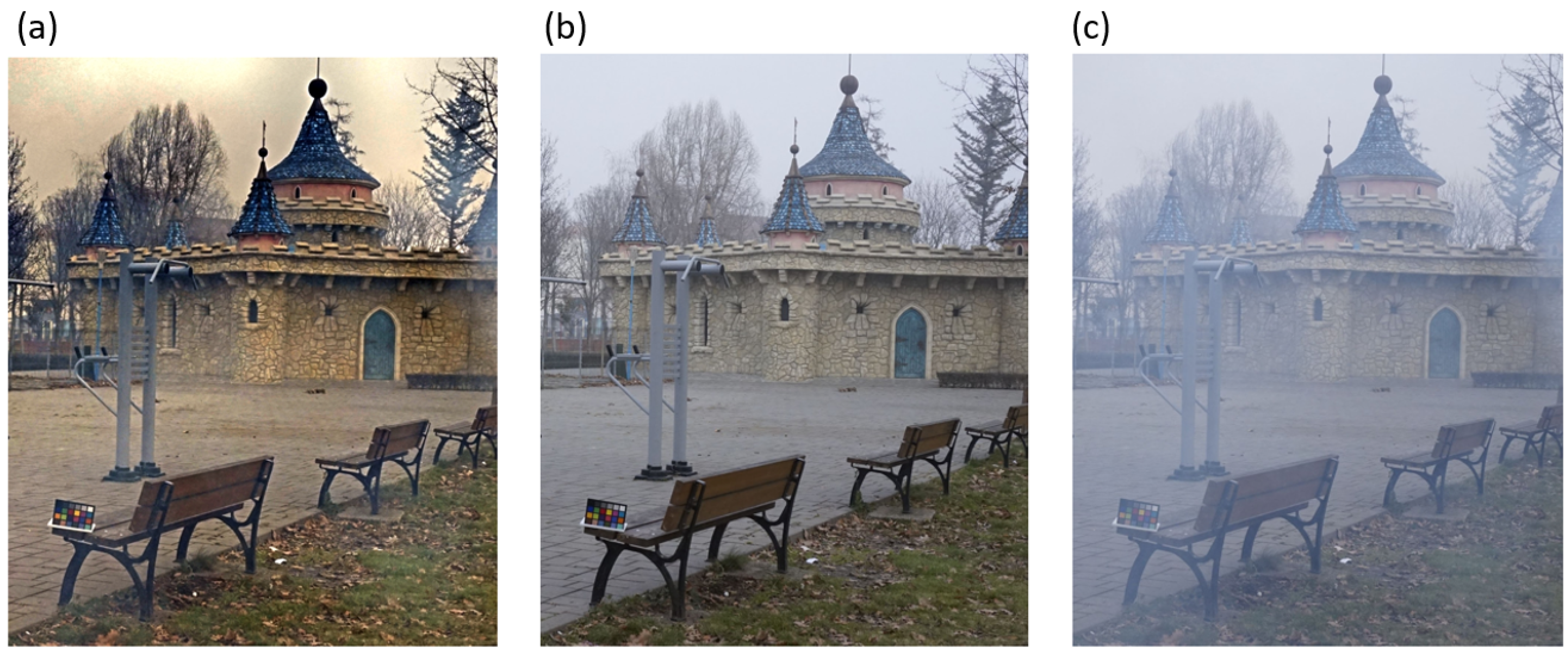
As Figure 1 shows, the main effect that hazy weather has on a scene is decreased luminance and contrast, which dramatically reduces the contours and textures of the scene. Maintaining defined contours in adverse weather conditions is key to reliable object recognition and segmentation, which are the basis of several applications. The visibility metrics we present in this work are based on gradient detection for image defogging evaluation. Our approach compares the gradient of the original foggy image to the gradient of its defogged counterpart, i.e., after the defogging procedure is complete. Hence, there is no need for a ground truth. Besides that, our method does not need to estimate any atmospheric parameter, which is difficult to obtain from a single RGB image and, in general, requires the sky to be present in the image.

Thus, as a first step, we need to obtain the derivative of both images (original and defogged), as can be seen in Figure 1. There are several well-known image processing operators that can be used to compute these derivatives. Some of the most frequently used are Canny [32], Roberts, Prewitt, and Sobel [33]. For our method, we used the Sobel edge detector [34] due to its simplicity. The horizontal and vertical derivatives were obtained by respectively convoluting the horizontal and vertical kernels on the image, as shown in Equation (1),

$$F_x=\left[\begin{array}{ccc}-1& 0& 1\\ -2& 0& 2\\ -1& 0& 1\end{array}\right]⊛I;F_y=\left[\begin{array}{ccc}-1& -2& -1\\ 0& 0& 0\\ 1& 2& 1\end{array}\right]⊛I,$$

(1)

where $F_x$ and $F_y$ are the corresponding horizontal and vertical derivatives of the image I resulting from the convolution (⊛) of both kernels. The final image integrating all gradients is retrieved following

$$F=\sqrt{F_x^2+F_y^2}.$$

(2)

Note that in any image, most of the pixels do not represent an edge, yielding small values in the processed gradient image. This can be appreciated in Figure 1, where the white pixels that represent null or negligible gradients are dominant in the image. Hence, we define a threshold value for the gradient values in order to differentiate the gradients of interest from the background (white). Defining a proper threshold is key to a reasonable evaluation of our metrics. A discussion about thresholding will be provided once Equation (4) is presented.

After obtaining the derivative of each image, we perform the relative difference between the gradient images of the fogged and its defogged counterpart pixel by pixel, as stated in Equation (3),

$$RD(u,v)=\left\{\begin{array}{c}\hfill {\displaystyle \frac{G_{def}(u,v)-G_{fog}(u,v)}{G_{fog}(u,v)}}{G}_{def}(u,v),G_{fog}(u,v)>\mathrm{threshold}\hfill \\ \hfill 0\mathrm{otherwise}\hfill \end{array}\right.,$$

(3)

where $RD(u,v)$ is the relative difference computed at pixel (u,v), $G_{def}(u,v)$ is the defogged gradient image and $G_{fog}(u,v)$ is the fogged gradient image.

Let us analyze the "relative difference image” obtained. This image has the same dimensions as both input images. Each pixel represents the relative difference between the corresponding pixels of both input gradient images. If the value of a pixel in the relative difference image is positive, the strength of the gradient in the defogged image has improved because the gradient value in the defogged image is larger than the gradient value in the original image. Otherwise, if the value of a pixel in the relative difference image is negative, the strength of the gradient has decreased after the defogging algorithm. Therefore, the value of the difference quantifies the improvement in gradient strength obtained after the defogging process. The larger the gradient strength, the more intense the contrast on the image; thus, the more feasible it is to perform perception tasks on it.

Once we compute the relative difference image $RD(u,v)$, we calculate its histogram while excluding the background pixels of the image, with the null values corresponding to those pixels below the threshold value. Figure 1 presents the resulting histogram (e) of the relative difference image obtained from images (c) and (d). The vast majority of edges in this image are better defined when fog is not present in the scene because of the defogging algorithm, as we would expect. Negative values close to zero in the histogram correspond to regions that have not been remarkably affected by fog or those in which the defogging process has introduced small variations in the gradient strength. Nonetheless, these pixels are quite residual compared to the rest. Note that positive pixels can reach values as large as 6, meaning a 6-fold improvement in the gradient strength.

At this point, the strategy of the gradient-based metrics becomes clear. However, we still need a scalar value to quantify the enhancement of the defogging procedure consistent with the information that can be graphically observed in the histogram presented in Figure 1. There are several options for obtaining this numerical value. Our proposal consists of calculating the weighted ratio between the positive part of the histogram and the whole one. Mathematically,

$$R={\displaystyle \frac{{\sum }_{i=0}^{\infty }{r}_i^{+}·h\left(r_i^{+}\right)-{\sum }_{i=0}^{\infty }\left|r_i^{-}\right|·h\left(r_i^{-}\right)}{{\sum }_{i=0}^{\infty }{r}_i^{+}·h\left(r_i^{+}\right)+{\sum }_{i=0}^{\infty }\left|r_i^{-}\right|·h\left(r_i^{-}\right)}}$$

(4)

where $r_i^{\pm }$ is the value of the relative difference, either positive or negative, and $h\left(r_i^{\pm }\right)$ corresponds to the histogram value of $r_i^{\pm }$—in other words, the total counts on the gradient image of such a value. R can take values from −1 to 1, being 1 when all the gradients have been enhanced and −1 when the defogging procedure has worsened all gradients of the image. The weighted character of the metrics is used to strengthen those gradients that have been greatly improved or worsened. If we compute the proposed metrics value for the example images shown in Figure 1 we get $R=0.9732$. This is a reasonable result since we are comparing a fogged image directly with its fog-free ground truth, mimicking an ideal defogging algorithm.

As previously mentioned, the threshold’s value in Equation (3) plays a key role in the metrics. This is left as a free parameter so the user can adapt the metrics to his dataset. A global threshold value that is too low might introduce severe noise while disregarding low-intensity gradients if too high. For the O-HAZE dataset [18], we empirically found that the best threshold value is 5% of the maximum gradient value present on the image. This value kept all relevant information related to gradients while disregarding background data. We determined this by maximizing the metrics’ result when a fog-free image is used as the perfect defogging method. The mean over the fog-free images of the O-HAZE dataset [18] is 0.956.

Fog is a highly dynamic phenomenon and it can present different behavior not only temporally, but also spatially within the image. This can lead to a certain degree of error when using a global threshold. This is why adaptive local thresholding [35] has also been studied, in particular Niblack’s local thresholding algorithm. With local thresholding, we can obtain more accurate measurements in non-homogenous fogged images. We achieved a mean value over the fog-free images of O-HAZE [18] of 0.979, higher than the optimized global relative threshold. The results presented in the paper are computed with Niblack’s method with a window size of 15 pixels and $k=-0.2$.

We would like to remark the following. As previously discussed, DNNs, and especially GANs [36], are currently used to tackle defogging. GANs are very useful when it comes to generating new data that resemble the data distribution they have learned from. This means that these networks tend to generate new features on images, leading to new contours that may produce better results in our metrics even if the defogging is poor.

These situations may occur with images lacking edge information. Under this condition, two scenarios could happen. First, the original haze-free image has no contours. In this case, fog will not be a problem since no information would be hidden due to fog. Moreover, the resulting defogged image will be very similar to the original hazy one because there is no element on the scene that needs to be improved. Second, the original haze-free scene has contours, but the fog is so dense that there is no visibility. This is a more delicate case since there are elements in the image that could be improved. Nevertheless, no realistic defogging method could recover any information under such conditions. Any contour generated under extremely low visibility can in practice be considered a “ghost” object as long as it appears in the image from nothing.

In our opinion, generating these “ghost” features in the image should directly discard the defogging method. Defogging is especially useful when it comes to increasing the performance of object detection and image segmentation, which will ultimately execute an action in an autonomous vehicle. Executing an action due to a ”ghost“ feature could be extremely dangerous. Thus, our metric works under the premise that no new features are added to the defogged image during the defogging procedure, and only already existing features are highlighted.

In 2008, Hautiére et al. [37] presented a reference-less metric that was based on a gradient comparison between the original hazy image and the defogged one. Specifically, it focuses on the new visible gradients that have appeared after the visibility enhancement. We hypothesize that any defogging method that generates new contours or gradients should be discarded. This decision is based purely on safety measurements, as the authors believe that the main application of defogging algorithms is autonomous systems. Among other differences in the algorithm, our metric differs from Hautiére in the sense that it deals with the up-to-date problems of the defogging issue.

A complete algorithm and a flowchart for the metrics computation are presented in Algorithm 1 and Figure 2, respectively.

Algorithm 1 Gradient-based metrics for image defogging without ground truth.

1: for $iteration=1,2,\dots ,T$ do 2:     $N,M\leftarrow Size\left(I_{fog}\right)$ 3:     Compute both gradient images $G_{fog}\leftarrow K_h,K_v,I_{fog}$, $G_{def}\leftarrow K_h,K_v,I_{def}$ (Equation (1)) 4:     Compute the relative difference image 5:     for $u=1,\dots ,N$ do 6:         for $v=1,\dots ,M$ do 7:            if $G_{fog}(u,v)>threshold\mathbf{and}{G}_{def}(u,v)>threshold$ then 8:                $RD(u,v)\leftarrow$ Equation (3) 9:            else 10:                $RD(u,v)\leftarrow 0$ 11:            end if 12:         end for 13:     end for 14:     $h\leftarrow histogram\left(RD\right)$ 15:     return $R\leftarrow$ Equation (4) 16: end for

4. Results and Discussion

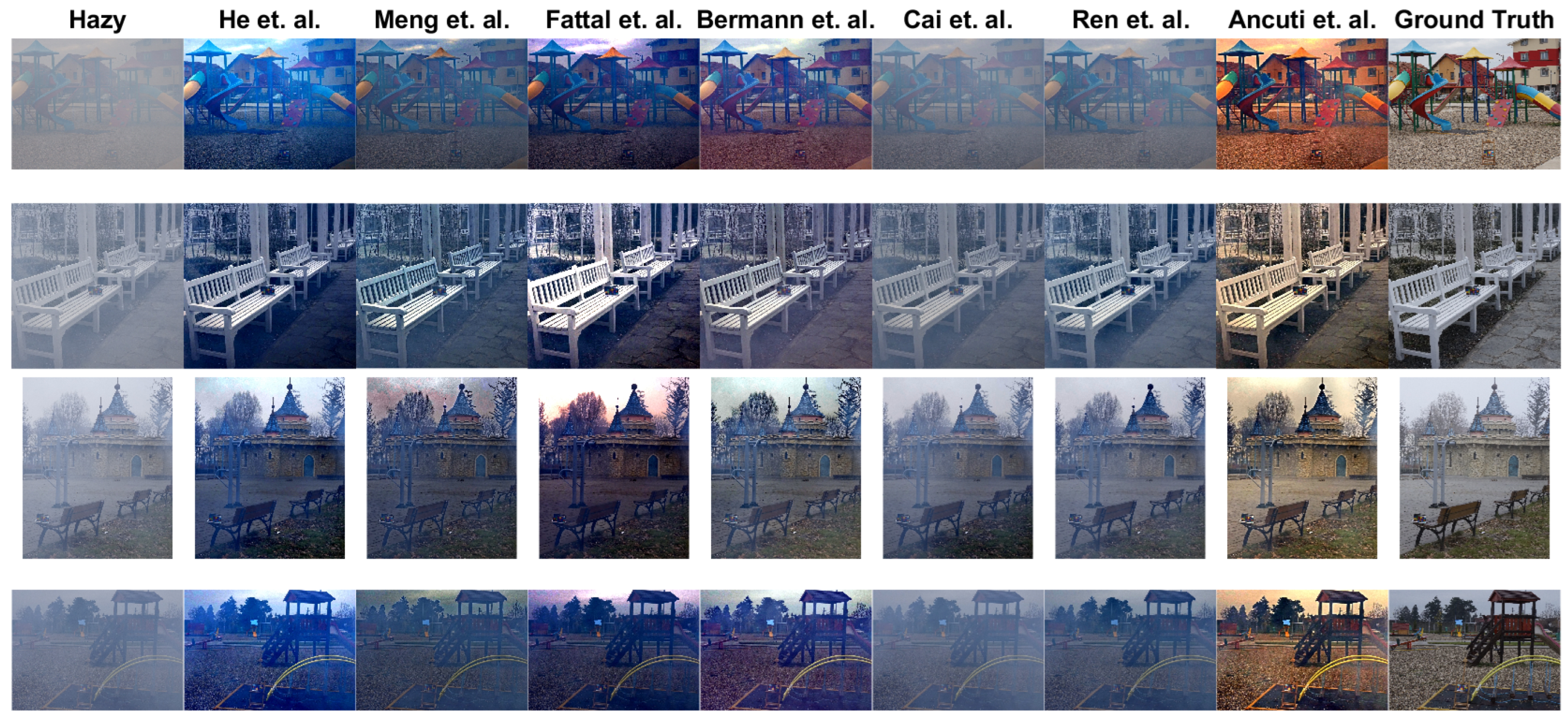
To validate our proposed metric, we tested it on the O-Haze dataset [18]. This dataset was used in the NTIRE 2018 challenge [6]. It consists of 45 outdoor scenes. Each fogged scene has its ground truth counterpart. Apart from that, the results of seven defogging methods provided by seven research groups were also facilitated with the dataset. Figure 3 shows some examples of the O-Haze dataset as well as the seven mentioned results of the defogging methods. We used our metrics to compare the results of some groups who participated in the challenge. During the NTIRE’18 defogging challenge, the groups received 35 fogged images with their respective ground truth for training their networks. They also received five more images for validation purposes and five more for testing; these images were evaluated by the jury. Again, the last 10 images had their respective ground truths delivered. To fully validate the effectiveness of our metrics, we used the abovementioned 45 scenes with every defogging method available, reaching up to 405 images. Apart from that, we also tested two state-of-the-art defogging evaluation metrics, FRFSIM [27], an FR-IQA metrics based on statistical behavior over human judgment on foggy scenes, and FADE [28], an NR-IQA fog density prediction model based on natural scene statistics, on the O-Haze dataset and compared the results with our own.

As mentioned above, the metrics used for evaluation in the NTIRE 2018 challenge were SSIM and PSNR, calculated relative to the ground truth image. The defogged images have 800 pixels of height or width at most, whereas both the ground truth and the original hazy images have greater resolutions, so we resized them to match the dimensions of the defogged image to enable proper comparison. The resize method used was the bi-cubic algorithm. After resizing, we computed the value of the SSIM, FADE, FRFSIM, and our proposed metrics for each scene and method. After that, we computed the mean over the 45 scenes to obtain a mean value of the defogging method for each criterion. Numerical values are shown in

Table 1. Mean over the 45 images of the O-Haze [18] dataset of SSIM (FR-IQA), our proposed metrics (NR-IQA), FADE (NR-IQA with natural scene statistics) and FRFSIM (FR-IQA with human judgment). The best- and worst-performing results are colored in green and red, respectively for each metrics. The upwards arrow means that better results show higher values. Contrary, the downward arrow means that better results show lower values.

	He et al.	Meng et al.	Fattal et al.	Bermann et al.	Cai et al.	Ren et al.	Ancuti et al.
SSIM↑	0.399	0.498	0.441	0.545	0.433	0.519	0.573
Ours↑	0.933	0.902	0.892	0.976	0.763	0.931	0.986
FADE↓	0.256	0.288	0.258	0.262	0.642	0.503	0.252
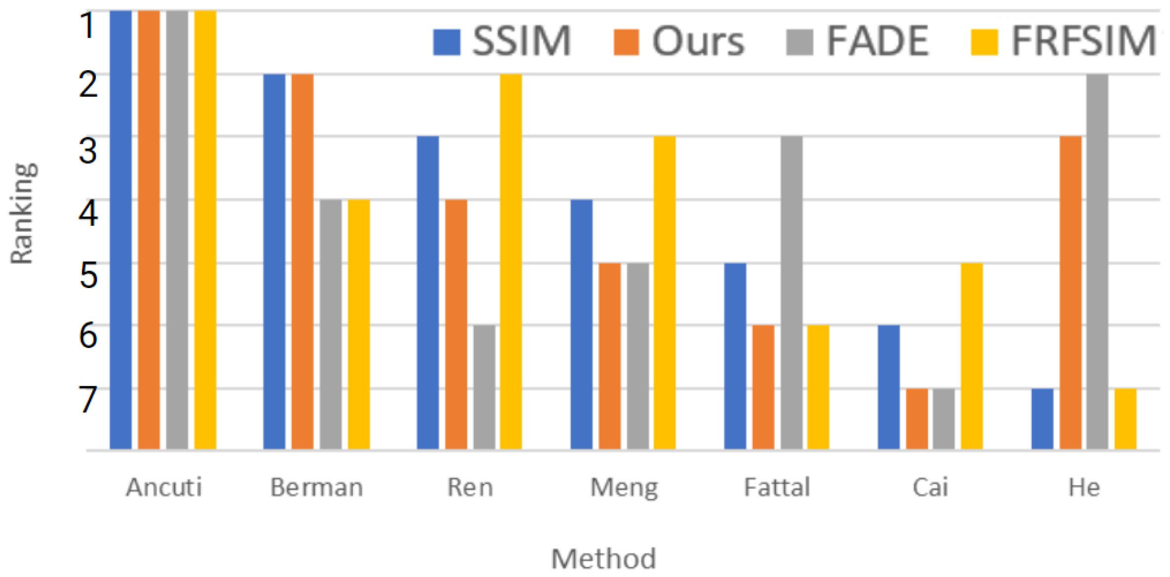
FRFSIM↑	0.340	0.461	0.352	0.443	0.352	0.468	0.480

, where the worst and best values of each metrics are plotted in red and green, respectively. The classification according to their ranking can be seen in Figure 4.

Table 1 and Figure 4 show relevant information. Firstly, every metric considers Ancuti’s as the best-performing defogging method. There is a dispute over which one comes in last place. On the one hand, our metrics and FADE, both NR-IQA, judge Cai’s as the worst method. On the other hand, SSIM and FRFSSIM state that He’s is actually the worst defogging procedure. Let us take a deeper insight into He’s case. When it comes to defogging and, especially, differentiating objects, He’s results are visibly better than Meng’s, Cai’s, or even Ren’s. Nevertheless, all previous groups are ahead of them when SSIM is applied. This can be explained by looking at the colors of each image and comparing them to the ground truth. The color aberration introduced by He is considered by SSIM and FRFSIM as a bad defogging method. On the contrary, our metrics strictly considers one of the most affected features by fog, the edges of objects, leading to a more reasonable position of He’s defogging method even without the need for a ground truth comparison.

As mentioned above, the metric used in the NTIRE’18 defogging challenge [6] was SSIM. Of the metrics used in the paper, our proposed one is the one that better resembles SSIM’s behavior. From SSIM’s perspective, FADE and FRFSIM are too harsh on Berman and give too much credit to Fattal or Cai. Yet, in our case, the only discrepancy with SSIM is the He exception discussed in the paragraph above.

Moreover, common metrics such as SSIM and PSNR reward similarity between the defogged image and its corresponding ground truth as they make a direct comparison between them. Nevertheless, many methods prioritize enhancing features such as contrast and illumination on the scene for better object detection/segmentation tasks [16]. This is positively considered by our metrics as gradients are key features for perception tasks. These enhancements may even produce greater values than their fog-free counterparts. For instance, as presented in Section 3, the mean value for the fog-free images of the O-HAZE [18] dataset is 0.979 whereas, as seen in Table 1, Ancuti’s [44] averaged 0.986. Ancuti’s defogged image presents regions with higher contrast than its ground truth counterpart. Looking at Figure 5, this is the case with trees and the sky or even with the leaves and the grass. This higher value in its gradients could lead to a higher value of the metrics. In this case, Ancuti’s proposal achieved 0.991 whereas the fog-free image achieved 0.965.

In Figure 6, we present a comparison between SSIM and our metrics by showing some examples of the relative difference image histogram and the defogged result for the images corresponding to different defogging methods in Figure 3. The figures in the last row represent the relative difference image ($RD(u,v)$). For ease of interpretation, the background is painted in white, with positive edge values in green and negative ones in red. The intensity of the edges is conserved so darker regions express little difference between the fogged and defogged images. An important feature to consider is that the better the defogging method, the more similarities can be found between the histogram of the defogged image and the ground truth, which has a larger positive area under the curve when our metrics value is closer to one. Also, our metrics’s values in this example agree with what we can observe: Ancuti’s method performs a better defogging job than Meng’s and Cai’s. However, the same thing cannot be said about the SSIM evaluation. Moreover, according to SSIM, Cai’s and Meng’s resulting defogged images are worse than the original hazy image, even though they visibly perform a good defogging task. Again, this proves that SSIM might not be the best metric for image-defogging evaluation in some cases.

5. Limitations

In Section 3, we have presented an algorithm that quantitatively judges the enhancement in the gradients of a defogging procedure without the need for training or any statistical bias. In Section 4, we proved its effectiveness. Nevertheless, the proposed metrics has some limitations that have been already discussed, but which we would like to sum up below.

Firstly, as mentioned before, our metrics cannot properly evaluate methods that generate gradients where there were none in the original scene. This is what we call “ghost” object generation, and it is especially an issue with generative methods such as GAN-like architectures. This issue is related to the extreme condition of zero visibility. No defogging method should generate gradients when there is no information available.

Secondly, computing the gradients of an image is known to be computationally expensive. Even though the presented metrics were designed to evaluate defogging methods before their potential implementations in autonomous vehicles, real-time capability would expand its usages. The computation time of the algorithm greatly depends on the threshold method and image resolution. On the one hand, global relative thresholds compromise precision in exchange for a faster computation time. On the other hand, local adaptive thresholds, such as Niblack’s method [35], provide finer results because they can adapt to the highly spatially dynamic features of fog. However, they generally require larger computation times, especially when applied to high-resolution images. For low-resolution images, the typical output from a neural network, the algorithm averages 0.02 s with a global threshold and over a second when a high-definition image is used. The computations were performed with an Intel Core i7-1170 at 2.50GHz. The metrics could be used in real-time conditions only if low-resolution images and a global threshold are used.

A solution to this problem might be using a neural network approach instead of a gradient-based method. Taking advantage of GANs’ generative capabilities, a feature map that could take into account the gradients of the image, as well as other features, could be obtained in a reduced amount of time. Nevertheless, GANs must be trained on huge annotated datasets, which is an important limitation in the defogging field, where paired fog and fog-free datasets are scarce. In fact, the limitation of defogging datasets was one of our main motivations for developing the proposed evaluation algorithm for defogging methods that does not need training or previous data whatsoever.

In addition, similarly to defogging, there also exist some lines of research that try to obtain a clear image from a rainy scene (deraining) [45] or from uncontrolled random noise (denoising) [46]. Although they share the same objective of obtaining a noise-free image from a noisy scene, there is a fundamental difference between defogging and denoising or deraining. Fog basically attenuates the gradients of the scene, whereas raindrops or random noise create gradients on top of a clear image. A good deraining or denoising method would actually reduce the gradients of the scene, resulting in a poor evaluation from our metrics. However, other lines of work such as blind deblurring [47] or super-resolution [48] may take advantage of our method, as its problem can be reduced to an enhancement and sharpening of gradients.

6. Conclusions

We have proposed a gradient-based metric for image defogging that does not need a ground truth image and measures the improvement in gradient strength on the defogged image without estimating any atmospheric parameter. We have also reviewed several state-of-the-art defogging techniques and metrics for evaluation. Finally, we compared our proposed metrics with the current metrics used in defogging challenges, SSIM, through the O-Haze dataset, as well as some state-of-the-art defogging evaluation metrics: FADE and FRFSIM. We compared the similarities and discrepancies between the metrics and concluded that the proposed metric properly measures visual enhancement of image defogging without any reference other than the original RGB fogged scene. It also improves the state of the art of NR-IQA defogging metrics as it is not biased by statistics or human judgment. This metric further enables progress in the defogging field because, in particular, it enables fast validation of defogging DNNs with unpaired fog and fog-free datasets. Additionally, other reference-less edge-sensitive image processing tasks like blind deblurring [47] and blind super-resolution [48] might use this metric for IQA evaluation as well. Based on the good results proved in this paper, proper adjustments to the metric’s algorithm might broaden its use for other low-vision tasks like the ones mentioned above.