Article

Dynamic Responses of 8-DoF Vehicle with Active Suspension: Fuzzy-PID Control

School of Mechanical Engineering, Anhui Institute of Information Technology, Wuhu 241100, China
*
Author to whom correspondence should be addressed.
World Electr. Veh. J. 2023, 14(9), 249; https://doi.org/10.3390/wevj14090249
Submission received: 27 July 2023 / Revised: 22 August 2023 / Accepted: 4 September 2023 / Published: 6 September 2023

Abstract

:
The driving smoothness of vehicles is heavily influenced by their suspension system, and implementing active suspension control can effectively minimize the vibration movement of the vehicle and ensure a comfortable driving experience. An 8-DoF active suspension model of the full vehicle is established, and a fuzzy-PID controller is designed to autonomously regulate the parameters of the PID controller. Using the MATLAB/Simulink environment, a simulation model for suspension is created, and the vibration characteristics of passive, PID control, and fuzzy-PID control suspensions are compared with the help of the continuous crossing road hump model and C-level road model as road inputs. The results show that the utilization of fuzzy-PID control considerably diminishes the vertical, pitch, and roll oscillations of the suspension body and modifies the suspension dynamic deflection and tire dynamic load in contrast to the other two scenarios, thus enhancing ride comfort. Fuzzy-PID control led to a decrease of approximately 40% in acceleration, 25% in suspension workspace, and 30% in tire deflection compared to passive suspension. In addition, the reduction in acceleration is about 20%, the reduction in suspension workspace is approximately 10%, and the reduction in tire deflection is about 15% compared to the PID control suspension system.

1. Introduction

Vehicles are one of the most prominent means of transportation in modern society, and the driving and riding experience of vehicles are receiving increasing attention. At present, vehicle suspension includes two types according to whether it has a control function: passive suspension and active suspension [1,2]. The parameters of each component of the passive suspension are determined, and it can only react passively to external forces based on its original design. The passive suspension cannot make timely changes according to the real-time conditions during the vehicle’s travel. The active suspension system and its control technology can address the limitation of the passive suspension system in adjusting to varying road conditions due to the rapid spread and development of electronics and intelligent control technology [3,4].
In classical fuel vehicles, the suspension is generally non-adjustable, so the comfort and sportiness of the vehicle are inherently contradictory. For this reason, air suspension systems [5] or electromagnetic induction suspension systems [6] have been added to advanced models of fuel vehicles to improve vehicle smoothness. Carbon neutrality and carbon peaking have accelerated the advent of the new energy vehicle era, which has been transformed to a great extent relative to classical fuel vehicles. Pure electric vehicles have mainly added an electric drive control system and eliminated the engine compared to classical fuel vehicles [7]. Electronic applications have come a long way in pure electric vehicles. The electrified drive-by-wire chassis is more suitable for electric vehicle development. The wire-controlled system eliminates some of the bulky and less accurate pneumatic, hydraulic, and mechanical connections and replaces them with electric-signal-driven sensors, control units, and electromagnetic actuators, so it has the advantages of compact structure, good controllability, and fast response speed [8]. The biggest advantage of the wire-controlled suspension system is that it can react according to different road conditions and driving status, which gives the car a better driving experience, and it is controlled by electric signals and is more intelligent. Advanced driver assistance systems (ADAS) are necessary to realize high-level autonomous driving for electric vehicles, so the wire-controlled chassis must be highly compatible with intelligent electric vehicles [9]. Wire-controlled suspension is becoming an indispensable core technology in the new energy vehicle industry.
The control method of vehicle suspension systems has been widely studied, and more and more new methods have been applied to active suspension systems. Active suspension control can be divided into the classical control algorithm [10], modern control algorithm [11], and intelligent control method [12]. Classical control methods include sky-hook control [13] and classical PID control [14]. Sky-hook control uses a negative feedback controller to generate a force proportional to the absolute speed of the controlled object, which can effectively suppress the resonance hump caused by the low-frequency vibration isolation mode without reducing the high-frequency vibration isolation capability. Ground-hook control [15] and mixed sky-hook and ground-hook control [16] are also derived based on sky-hook control. Classic PID control is a control algorithm that combines proportion, integration, and differentiation in a closed-loop system, which can automatically correct the control system accurately and quickly. Modern control algorithms include optimal control [17], adaptive control [18], robust control [19], and sliding mode variable structure control [20]. Optimal control is to find out the allowable control rule, make the dynamic system transfer from the initial state to a required terminal state, and ensure that a required performance index reaches the minimum (or large). It mainly includes linear quadratic form optimal control [21] and the dynamic programming method [22]. Adaptive control includes model reference adaptive control [23] and self-tuning control [24], and its main control idea is to modify the characteristics of the control object itself to adapt to changes in the dynamic characteristics of the object and disturbance. Robust control introduces some robust designs into the control system to make the system stable under the influence of uncertainties, mainly including the Kharitonov interval theory [25], structural singular value theory (μ theory) [26], and H control theory [27]. Sliding mode variable structure control can continuously change purposefully according to the current state of the system (such as deviation and its derivatives of each order) in the dynamic process, forcing the system to move according to the state track of the predetermined sliding mode, which includes single-mode sliding [28], multi-mode sliding [29], super-twisting sliding [30], and adaptive sliding [31]. Intelligent control methods include fuzzy control [32], neural network control [33], optimization control based on the genetic algorithm [34], expert control [35], and hierarchical intelligent control [36]. Fuzzy control is an intelligent control method that imitates human fuzzy reasoning and decision-making processes. Neural network control can perform neural network model identification on complex nonlinear objects that are difficult to accurately model. The optimization control based on a genetic algorithm simulates biological evolution processes such as natural selection, heredity, and mutation. Expert control combines the theory and technology of expert systems with control theory, methods, and technologies, imitating the experience of experts in unknown environments. Based on adaptive control and self-organizing control, hierarchical intelligent control is divided into the organizational level, coordination level, and execution level according to the level of intelligent control, and these three levels follow the principle of intelligent descending and increasing accuracy.
Numerous scholars have consistently investigated the research area of active suspension technology to enhance the overall performance of vehicles. The control algorithm is the core of active suspension research, which is an effective means to enable active suspension to achieve ideal vibration damping. The research focus on intelligent control has gradually shifted to the fusion of classical or modern control methods and intelligent control methods, which utilize the adaptive ability of intelligent control methods to further improve the performance of the classical controller. Senthilkumar and Sivakumar [37] introduced fuzzy control to the continuously damped automotive suspension system and solved the multi-variable dynamic characteristics of the active suspension system. Bozorgvar and Zahrai [38] designed the suspension fuzzy logic controller and optimized the control rules with an enhanced genetic algorithm. Kaldas et al. [39] developed a semi-active suspension system controller using fuzzy control theories together with the Kalman filter. Chen et al. [40] integrated a neuro-fuzzy (NF) adaptive controller with a modeling neural network (MNN). An optimal adaptive fuzzy controller was presented by Mahmoodabadi and Javanbakht [41], which utilized the gravitational search algorithm (GSA) to identify the optimal controller parameters. Zhi et al. [42] proposed a variable-domain fuzzy control method to optimize the suspension parameters. Soleymani et al. [43] designed two independent fuzzy controllers for the front and rear suspensions using an 8-DoF (degree of freedom) full-vehicle model and used a multi-objective Pareto optimal solution to tune the parameters of the fuzzy controller. Eltantawie [44] designed a decentralized neuro-fuzzy controller using a magnetorheological damper as a semi-active control device. Ahmed et al. [45] proposed a fuzzy DE-PID controller based on an improved DE (differential evolution) algorithm to enhance the control gain. Kumar et al. [46] designed a fuzzy logic controller whose input data are the velocity and acceleration of front and rear wheels. Na et al. [47] incorporated prescribed performance functions into the control implementation, which preserves transition and steady-state suspension performance. Fang and Bai [48] investigated adaptive fuzzy fault-tolerant control through a sensor fault compensation approach. Li et al. [49] considered the sampled Takagi-Sugeno (T-S) fuzzy semi-vehicle active suspension system to establish a continuous system with input delay. The online self-tuning output of the proportional coefficients of the fuzzy sliding mode controller was achieved by Hsiao and Wang [50] through the use of a fuzzy control approach. Jia et al. [51] tackled the fixed time control problem of suspension systems by using an event-triggered adaptive fuzzy control method. Hu and Yang [52] proposed an improved fuzzy-PID-integrated control strategy. Moaaz et al. [53] compared the jump vibration performance of magnetorheological semi-active suspension, passive suspension, and optimized passive suspension.
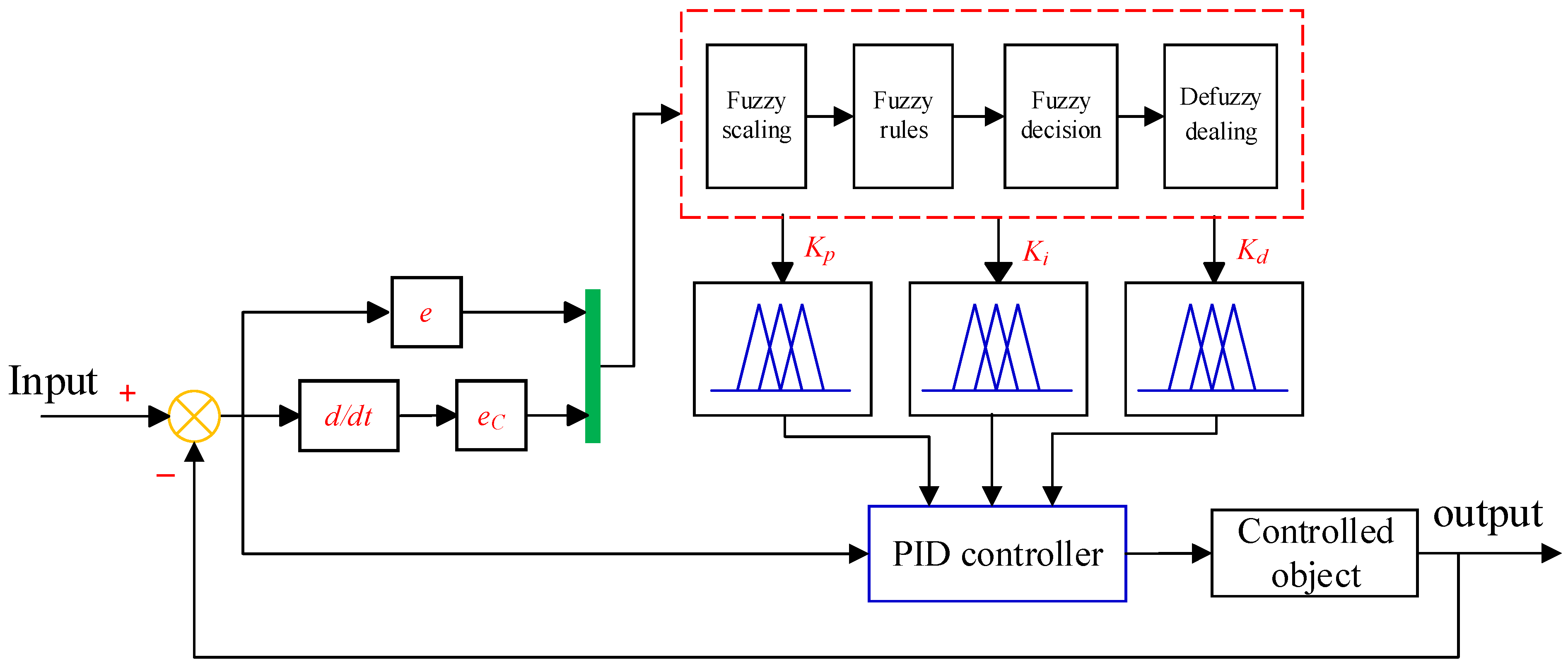
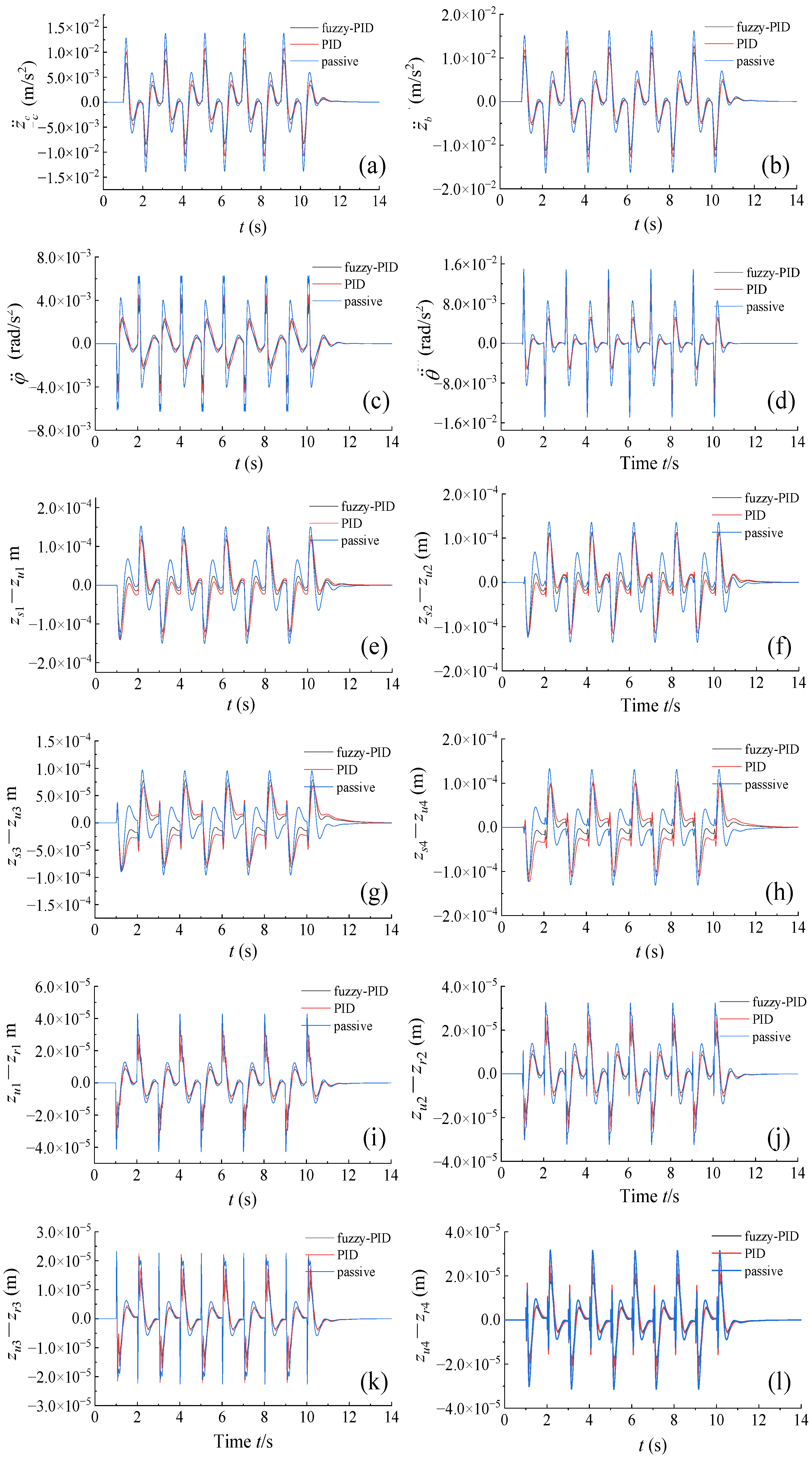
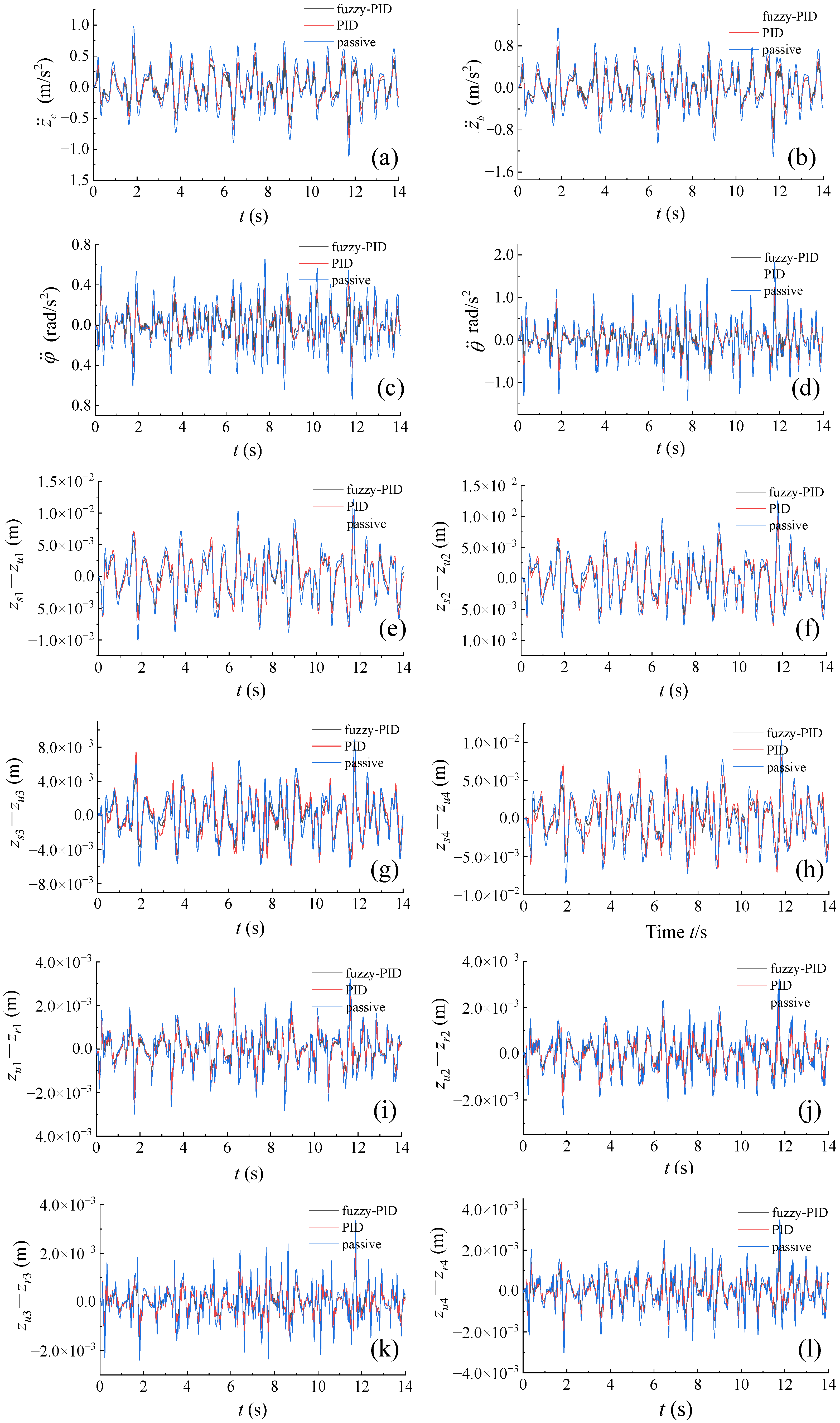
By isolating the vehicle body from road disturbances, the suspension system enhances passenger comfort, safety, and road handling. In the PID controller, the control quality is less sensitive to the change of the controlled object. The PID controller is linear, and it may not perform well in practice due to the nonlinearity of most controlled objects, resulting in decreased accuracy. The offline design of the PID algorithm is inadequate for handling the unexpected vibrations that occur when driving a vehicle under different road conditions. Therefore, a fuzzy-PID controller is proposed in this paper, which can further improve the performance of the active suspension system according to the fuzzy control rules. An 8-DoF model of full-vehicle active suspension is established, and the fuzzy-PID controller is designed by automatically adjusting the parameters of the PID controller. A suspension simulation model is established in the MATLAB/Simulink environment, and the vibration characteristics of the passive, PID control, and fuzzy-PID control suspensions are compared under the continuous crossing road hump model and C-level road model as control inputs.

2. Mathematical Model of Suspension

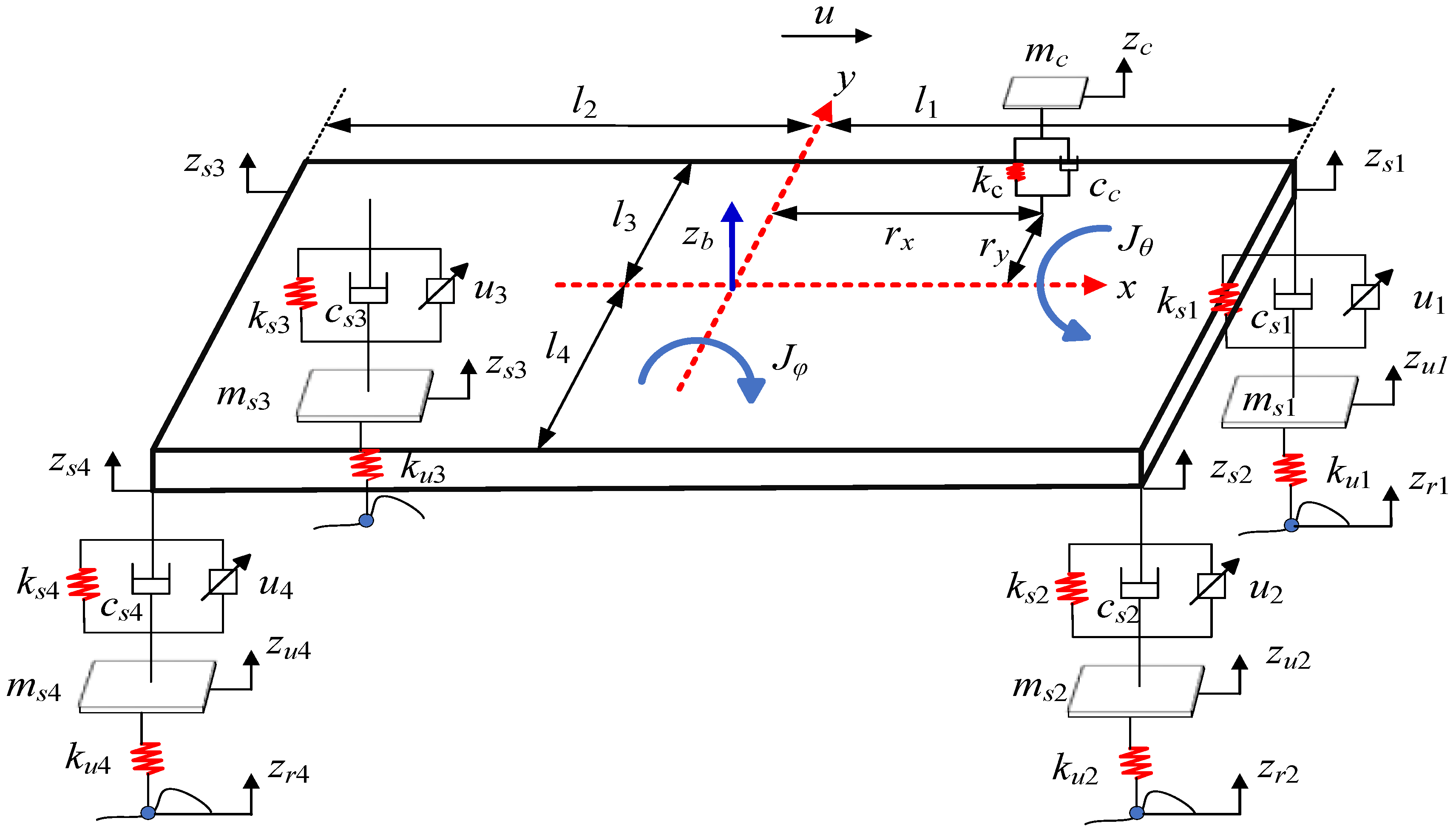
The 8-DOF dynamic model of the full vehicle comprehensively considers the effects of vertical, pitch, and roll motions. To reduce and suppress the vibration and impact caused by uneven road surfaces, the active suspension system is employed. The dynamic features of the vehicle’s suspension are fully represented by the active suspension, which actively controls the vibration that is transmitted to the human body. Based on the above analysis, the simplified physical model is shown in Figure 1, and the corresponding mathematical model is established. Due to the longitudinal motion of the vehicle, when the pitch angle θ and roll angle φ change in a small range of change, the approximate kinematics between the vertical displacement zsi of the suspension and the vertical displacement zxy of the seat system position are as follows:
z s 1 = z b l 1 θ + l 3 φ ,
z s 2 = z b l 1 θ l 4 φ ,
z s 3 = z b + l 2 θ + l 3 φ ,
z s 4 = z b + l 2 θ l 4 φ ,
z x y = z b r x θ + r y φ .
The equations below are derived from the kinematics and dynamics theory of the 8-DOF full-vehicle model:
(1)
Equation for the motion of the center of mass of the human-chair system:
m c z ¨ c = k c ( z c z x y ) c c ( z ˙ c z ˙ x y ) ,
(2)
Equation for the motion of the center of mass of the suspension body:
m b z ¨ b = i = 1 4 [ k s i ( z s i z u i ) c s i ( z ˙ s i z ˙ u i ) u i ] + k c ( z c z x y ) + c c ( z ˙ c z ˙ x y ) ,
(3)
Differential equation for suspension pitch rotation:
J θ θ ¨ = i = 1 , 2 l 1 [ k s i ( z s i z u i ) + c s i ( z ˙ s i z ˙ u i ) + u i ] i = 3 , 4 l 2 [ k s i ( z s i z u i ) + c s i ( z ˙ s i z ˙ u i ) + u i ] r x [ k c ( z c z x y ) + c c ( z ˙ c z ˙ x y ) ] ,
(4)
Differential equation for suspension roll rotation:
J φ φ ¨ = i = 1 , 3 l 3 [ k s i ( z s i z u i ) + c s i ( z ˙ s i z ˙ u i ) + u i ] i = 2 , 4 l 4 [ k s i ( z s i z u i ) + c s i ( z ˙ s i z ˙ u i ) + u i ] r y [ k c ( z c z x y ) + c c ( z ˙ c z ˙ x y ) ] ,
(5)
Equations for the movement of four unsprung masses:
m u i z ¨ u i = k s i ( z s i z u i ) + c s i ( z ˙ s i z ˙ u i ) k u i ( z u i z r i ) + u i   ,   i = 1 , , 4 ,
where zc is the vertical displacement of the human, zb represents the vertical displacement of the center of mass of the vehicle, zsi denotes the vertical displacement of the suspension, zui is the vertical displacement of the tire, θ means the pitch angle, φ is the roll angle, zxy is the vertical displacement of the human-chair system, zri represents the vertical displacement excited by the road surface, and ui is the suspension control input. The left-front wheel, right-front wheel, left-rear wheel, and right-rear wheel correspond to subscripts 1, 2, 3, and 4, respectively. Table 1 provides parameters for the inherent characteristics of the full vehicle.
For simplicity, Equations (1)–(10) are written in matrix form:
M X ¨ + C X ˙ + K X = B U + W Z
where state variables X = [zc, zb, θ, φ, zu1, zu2, zu3, zu4]T, control variables U = [u1, u2, u3, u4]T, and excitation variables Z = [zr1, zr2, zr3, zr4]T. The mass matrix M, damping matrix C, stiffness matrix K, control matrix B, and excitation matrix W are denoted as follows:
M = d i a g ( m c ,   m b ,   J θ ,   J φ ,   m u 1 ,   m u 1 ,   m u 1 ,   m u 1 ) , C = ( C 1 C 2 ) , K = ( K 1 K 2 ) , B = ( B 1 B 2 ) , W = ( 0 4 × 4 W 1 ) ,
where
C 1 = ( c 11 c 12 c 13 c 14 0 0 0 0 c 21 c 22 c 23 c 24 c 25 c 26 c 27 c 28 c 31 c 32 c 33 c 34 c 35 c 36 c 37 c 38 c 41 c 42 c 43 c 44 c 45 c 46 c 47 c 48 ) , C 2 = ( 0 c 52 c 53 c 54 c 55 0 0 0 0 c 62 c 63 c 64 0 c 66 0 0 0 c 72 c 73 c 74 0 0 c 77 0 0 c 82 c 83 c 84 0 0 0 c 88 ) , K 1 = ( k 11 k 12 k 13 k 14 0 0 0 0 k 21 k 22 k 23 k 24 k 25 k 26 k 27 k 28 k 31 k 32 k 33 k 34 k 35 k 36 k 37 k 38 k 41 k 42 k 43 k 44 k 45 k 46 k 47 k 48 ) , K 2 = ( 0 k 52 k 53 k 54 k 55 0 0 0 0 k 62 k 63 k 64 0 k 66 0 0 0 k 72 k 73 k 74 0 0 k 77 0 0 k 82 k 83 k 84 0 0 0 k 88 ) , B 1 = ( 0 0 0 0 1 1 1 1 l 1 l 1 l 2 l 2 l 3 l 4 l 3 l 4 ) , B 2 = ( 1 0 0 0 0 1 0 0 0 0 1 0 0 0 0 1 ) , W 1 = ( k u 1 0 0 0 0 k u 2 0 0 0 0 k u 3 0 0 0 0 k u 4 ) ,
in which (since the itemization of damping matrix C is almost the same as that of stiffness matrix K, the itemization of stiffness matrix K is omitted)
c 11 = c c , c 12 = c c , c 13 = r x c c , c 14 = r y c c , c 21 = c 12 ,   c 22 = c c + c s 1 + c s 2 + c s 3 + c s 4 , c 23 = r x c c l 1 c s 1 l 1 c s 2 + l 2 c s 3 + l 2 c s 4 , c 24 = r y c c + l 3 c s 1 l 4 c s 2 + l 3 c s 3 l 4 c s 4 , c 25 = c s 1 , c 26 = c s 2 , c 27 = c s 3 , c 28 = c s 4 , c 31 = c 13 , c 32 = c 23 ,   c 33 = r x 2 c c + l 1 2 c s 1 + l 1 2 c s 2 + l 2 2 c s 3 + l 2 2 c s 4 , c 34 = r x r y c c l 1 l 3 c s 1 + l 1 l 4 c s 2 + l 2 l 3 c s 3 l 2 l 4 c s 4 , c 35 = l 1 c s 1 , c 36 = l 1 c s 2 , c 37 = l 2 c s 3 , c 38 = l 2 c s 4 , c 41 = c 14 , c 42 = c 24 , c 43 = c 34 , c 44 = r y 2 c c + l 3 2 c s 1 + l 4 2 c s 2 + l 3 2 c s 3 + l 4 2 c s 4 , c 45 = l 3 c s 1 , c 46 = l 4 c s 2 , c 47 = l 3 c s 3 , c 48 = l 4 c s 4 , c 52 = c 25 , c 53 = c 35 , c 54 = c 45 , c 55 = c s 1 , c 62 = c 26 , c 63 = c 36 , c 64 = c 46 , c 66 = c s 2 , c 72 = c 27 , c 73 = c 37 , c 74 = c 47 , c 77 = c s 3 , c 82 = c 28 , c 83 = c 38 , c 84 = c 48 , c 88 = c s 4 , k 55 = k s 1 + k u 1 , k 66 = k s 2 + k u 2 , k 77 = k s 3 + k u 3 , k 88 = k s 4 + k u 4 .
Let X ˜ = [ X ˙ X ] T be the state vector, the system dynamics Equation (11) can be converted into first-order dynamics as follows:
X ˜ ˙ = G ˜ X ˜ + B ˜ U + W ˜ Z
where G ˜ = ( M 1 C M 1 K I 8 0 8 × 8 ) , B ˜ = ( M 1 B 0 8 × 4 ) , W ˜ = ( M 1 W 0 8 × 4 ) .
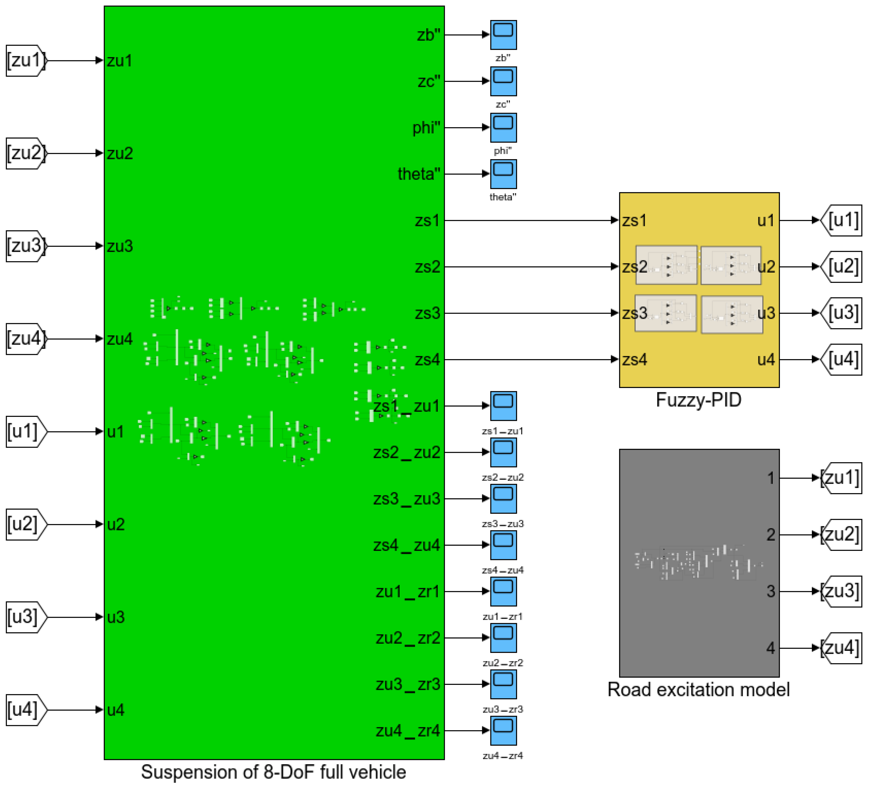
The mathematical model of the active suspension of the 8-DOF full vehicle is established using MATLAB/Simulink, as displayed in Figure 2.

3. Road Excitation Models

3.1. Continuous Crossing Road Hump Model

When the vehicle is driving through speed bumps at high speed, the suspension system will be impacted several times or even a dozen times higher than normal driving, which will seriously affect the service life of springs, brackets, and other components. However, speed bumps on the road are a very common road condition. It is of practical significance to study the smoothness of the vehicle by studying the continuous crossing road hump model.
The continuous crossing road hump model for front and rear wheels is as follows [54]:
q f ( t ) = q r ( t + ( l 3 + l 4 ) / u ) = { 0 , T i t T i + 1 z , T i + 1 < t < T i + 2 , i   = 1 , 3   , 2 i index 1 ,
where qf and qr denote the longitudinal slope curves of the front and rear wheels, respectively, iindex is the index of the speed bump, and z is the height of the speed bump z = 0.05 m.

3.2. C-Level Road Model

The change q(I) in the height q of the pavement relative to a reference plane along the roadway alignment I is known as the longitudinal slope curve of the pavement. The excitation process of the road surface is a stochastic process, and the pavement power spectral density Gq(n) of the longitudinal slope curve q(I) is used as the fitted expression by the following equation:
G q ( n ) = G q ( n 0 ) ( n / n 0 ) W ,
where n represents the spatial frequency, Gq(n0) denotes the coefficient for pavement unevenness at a spatial frequency of n0, n0 = 0.1 m−1 means the reference spatial frequency, and W = 2 is the frequency index.
For the input of the vehicle vibration system, in addition to the road roughness, the effect of vehicle speed should also be considered. The frequency domain power spectral density must be derived from the spatial frequency power spectral density based on the speed of the vehicle. If a vehicle drives over an uneven road surface with spatial frequency n at a certain speed u, the angular frequency ω of the road surface input is
ω = 2 π u n .
The relationship between the road spectral density Gq(n) represented by n and the power spectral density Gq(ω) represented by ω is as follows:
G q ( ω ) = G q ( n ) / 2 π u n .
Since the pavement spectrum is approximately horizontal in the low-frequency range, the lower cutoff frequency ω0 can be introduced into the power spectral density Gq(ω). So, the power spectral density Gq(ω) can be written as
G q ( ω ) = ( 2 π ) 2 G q ( n 0 ) n 0 2 u ω 2 + ω 0 2 ,
where ω0 = 2πn00u denotes the cutoff frequency, and n00 = 0.01 m−1 represents the cutoff spatial frequency under road roughness.
The power spectral density of the output power produced by a unit white noise Sω = 1 through a linear system is equivalent to the spectral density of the road surface, as per the filtered white noise technique [55]. Additionally, the frequency domain response function of the linear system H1(jw) is assumed to be as follows:
H 1 ( j ω ) = a u b + j ω ,
where a = 2πn00, and b = 2πn0(Gq(n0)u)1/2. Then, the output power spectral density is as follows:
G q ( ω ) = | H 1 ( j ω ) | 2 S ω .
Thus, the differential equation of linear system H1() is as follows:
q ˙ ( t ) = 2 π n 00 u · q ( t ) + 2 π n 0 G q ( n 0 ) u · w ( t ) ,
where w(t) is the unit white noise function of unit white noise Sω. More information about the time-domain model of single-wheel road excitation based on filtered white noise can be found in [56].
The previous description only considers the self-spectrum of one wheel, and the full-vehicle 8-DOF model needs to consider the vibration transmission of four wheel inputs. It is assumed that the rear wheels lag behind the front wheels by a certain length. Furthermore, the statistical characteristics of the unevenness between the left and right wheels are described by the mutual power spectral density or coherence function between two wheels.

3.3. Time Domain for Front and Rear Wheels on the Same Track

The time-domain model of single-wheel road excitation in Equation (20) is simplified as follows:
q ˙ ( t ) = a u · q ( t ) + b · w ( t ) .
Assuming that the vehicle is traveling in a straight line at constant speed, and the time delay caused by the excitation of the front and rear wheels on one side is T = (l1 + l2)/u. The first-order Pade approximate delay transfer function eTs is used to represent the time delay effect of the rear wheels on the front wheels [57], as shown below:
H 2 ( s ) = ( 1 T s 2 ) / ( 1 + T s 2 ) .
where s is the Laplace operator. It is obvious that ||H2(s)|| = 1 is an all-pass system where the amplitude of the frequency component remains unchanged. Then Gqr(ω) = |H2()|2Gqf(ω) = Gq(ω), and Gqf(ω) is the power spectral density function of the front wheel. The time-domain delay model of the rear wheel is obtained from this transfer function:
q ˙ r = 2 T q r q ˙ f + 2 T q f ,
where subscripts f and s denote front and rear wheels, respectively. In summary, the time-domain model of road excitation for the front and rear wheels on the same track is rewritten as
( q ˙ f q ˙ r ) = ( a u 0 a u + 2 T 2 T ) ( q f q r ) + ( b b ) w ( t ) .

3.4. Time Domain for Left and Right Wheels at the Same Axle

Experiments have proven that there is a correlation between left and right wheels at the same axle. The coherence function cohlr(ω) of left and right wheels at the same axle is defined as [58]
c o h l r 2 ( ω ) = | G l r ( ω ) | 2 G q l ( ω ) G q r ( ω ) 1 ,
where Glr(ω) is the spectral density of the cross power between the left and right wheels. Assuming that the self spectra ql(t) and qr(t) of the left and right wheels are the same, and the phase spectrum between the two wheels is equal to zero, then the following relationship is established:
G l r ( ω ) = | G l r ( ω ) | = c o h l r ( ω ) G q ( ω ) .
With the left wheel ql(t) as a reference, the above formula Glr(ω) can be considered as the output of Gq(ω) through a linear system H3(), and the amplitude frequency characteristic of this frequency response function ||H3()|| is equal to cohlr(ω). Assuming that the transfer function between the left and right wheels ql(t) and ql(t) is approximated by a second-order rational fraction, we obtain
H 3 ( s ) = a 0 + a 1 s + a 2 s 2 b 0 + b 1 s + b 2 s 2 ,
where a0 = 3.1851, a1 = 0.2063, a2 = 0.0108, b0 = 3.223, b1 = 0.59, and b2 = 0.0327 [57,59]. Transforming the above transfer function into the state equation between the left and right wheels and adding the intermediate state variable ξ(t) = [ξ1(t), ξ2(t)]T, we can get
( ξ ˙ 1 ( t ) ξ ˙ 2 ( t ) ) = ( b 1 b 2 b 0 b 2 1 0 ) ( ξ 1 ( t ) ξ 2 ( t ) ) + ( 1 b 2 0 ) q l ( t ) .
The time-domain expression for the right wheel track is
q r ( t ) = ( a 1 a 2 b 1 b 2 a 0 a 2 b 0 b 2 ) ( ξ 1 ( t ) ξ 2 ( t ) ) + a 2 b 2 q l ( t ) ,
where subscripts f and r denote left and right wheels, respectively.

4. Fuzzy-PID Control

4.1. Design of Fuzzy Controller

The PID regulation technique is commonly used for its advantages of simple structure, excellent robustness, and good reliability. The control algorithm of PID is as follows:
u ( t ) = r K p e ( t ) + s K i e ( t ) d t + t K d d e ( t ) d t ,
where u(t) is the control output, e(t) is the system error, and r, s, and t are gain coefficients. The proportional, integration, and differential coefficients of PID regulation are indicated by Kp, Ki, and Kd, respectively, as shown in Figure 3.
Fuzzy-PID control refers to the real-time optimization of PID parameters. Since the full-vehicle model of suspension is selected, four fuzzy controllers will be designed for four support points of the vehicle body, as shown in Figure 4a. Each controller takes the difference e i = 0 z ˙ s i (i = 1, 2, 3, and 4) between the speed of the support point of the vehicle body and the ideal speed and the first derivative eCi as the inputs of fuzzy-PID. The force ui of the actuator is used as the controller output. The value of the ideal speed is always equal to 0. Figure 3 displays the three outputs of the fuzzy controller, namely Kp, Ki, and Kd.
Fuzzy reasoning employs fuzzy variables, whereas the input and output quantities of the suspension system are mathematical quantities. Therefore, the prerequisite for using fuzzy control is to fuzzify the mathematical quantities. Based on the passive suspension model, the suspension system takes the established road excitation model as input to obtain the amplitude range of the vertical vibration velocity z ˙ s i and its change rate of the four support points of the vehicle body, which are ei = [−0.1 m/s, 0.1 m/s], eCi = [−1.5 m/s2, 1.5 m/s2], and the range of the force of the actuator is ui = [−200 N, 200 N].
As illustrated in Figure 4b, the input quantities ei and eCi are transformed into integer theoretical domains {−3, −2, −1, 0, 1, 2, 3} with quantization factors of 30 and 2, respectively. The outputs Kp, Ki, and Kd of the fuzzy controller are {−1, −2/3, −1/3, 0, 1/3, 2/3, 1}, and r = 1000, s = 6000, and t = 20 are set. To represent the fuzzy states of the input–output, a total of seven subsets that are fuzzy are used, namely {NB, NM, NS, ZE, PS, PM, PB}.
The membership function μ of the input–output of the fuzzy controller are both expressed as Gaussian functions:
μ ( y , σ , c ) = e ( y c ) 2 2 σ 2 ,
where σ is the shape of the function curve, and c is the center position of the function curve. Figure 4c,d are the Gaussian function images of the designed input and output, respectively. Defuzzification is the conversion of the fuzzy values obtained by inference into explicit control signals as the input values of the system. There are various methods of defuzzification, the most common ones are the maximum subordination method, centroid method, and weighted average method. Defuzzification is carried out using the centroid approach due to its ability to produce a smooth output. The expression for the centroid method is as follows:
y = k = 1 n y k μ ( y k ) / k = 1 n μ ( y k ) ,
where yk is the input values of the fuzzy system, and μ(yk) is the membership value of yk.

4.2. Fuzzy Rules of Fuzzy Controller

Multiple interrelated simulation models are established using various fuzzy control rules, taking into account the trend of error changes and human engineering experience to enhance the control output. Fuzzy controllers have the benefit of not needing a precise model of the object being controlled, instead relying on human control experience. The robustness of the fuzzy controller makes it particularly well-suited for controlling systems with strong nonlinearity, time variation, and significant delays. The control rules for the three coefficients Kp, Ki, and Kd of fuzzy-PID control are determined by the fuzzy controller and presented in Table 2, Table 3 and Table 4 [60]. Lu et al. [60] showed that these fuzzy control rules can be applied to the pulsed MIG welding of aluminum alloys, which can serve as an important reference source for us to verify the stability of fuzzy control rules. Figure 5 displays the curve of the fuzzy controller’s relationship, which was designed using two input and three output parameters.

4.3. Structure Analysis and Stability

As described in Section 4.2, in general, the Mamdani-type fuzzy control law can be described by IF-THEN rules associated with linguistic variables [61], as follows:
Rule Rk: IF x1 is 𝒩1k AND x2 is 𝒩2k AND … xm is 𝒩mk
THEN yk is 𝒲k, k = 1, 2, …, n,
where Rk is the kth control rule, 𝒲k and 𝒩jk, j = 1, 2, …, m, denote fuzzy sets, and n is the total number of fuzzy rules. The Zadeh fuzzy logic AND operator (i.e., min()) is used to realize the AND operations in the above-mentioned rules. Thus, the membership value of yk can be written as
μ W k ( y k ) = min { μ N 1 k ( x 1 ) , μ N 2 k ( x 2 ) , , μ N m k ( x m ) } ,
where μ𝒩 is the membership function of variable x. Combining Equations (30) and (32), and replacing x1 and x2 with ei and eCi, the output state of the fuzzy system is
K p i = k = 1 n y k μ P k ( y k ) / k = 1 n μ P k ( y k ) ,
K i i = k = 1 n y k μ I k ( y k ) / k = 1 n μ I k ( y k ) ,
K d i = k = 1 n y k μ D k ( y k ) / k = 1 n μ D k ( y k ) ,
where P , I , and D are fuzzy sets of Kp, Ki, and Kd, respectively. By bringing Equations (34)–(36) into Equation (30), the control output ui(t) can be obtained.
The input fuzzy subset divides the fuzzy space into 36 subspaces, as shown in Figure 6. If a dynamic system described by Equation (12) is uniformly asymptotically stable in the large, then all fuzzy controllers in the subspaces require asymptotic stability. Within each subspace, four fuzzy rules are activated. For example, in subspace S1, the activated fuzzy rules are as follows (seeing Table 2, Table 3 and Table 4):
(1)
For Kp,
Rule R1: IF e is NB AND ec is NB, Then Kp is PB,
Rule R2: IF e is NB AND ec is NM, Then Kp is PB,
Rule R3: IF e is NM AND ec is NB, Then Kp is PB,
Rule R4: IF e is NM AND ec is NM, Then Kp is PB,
(2)
For Ki,
Rule R1: IF e is NB AND ec is NB, Then Ki is NB,
Rule R2: IF e is NB AND ec is NM, Then Ki is NB,
Rule R3: IF e is NM AND ec is NB, Then Ki is NB,
Rule R4: IF e is NM AND ec is NM, Then Ki is NB,
(3)
For Kd,
Rule R1: IF e is NB AND ec is NB, Then Kd is PS,
Rule R2: IF e is NB AND ec is NM, Then Kd is PS,
Rule R3: IF e is NM AND ec is NB, Then Kd is NS,
Rule R4: IF e is NM AND ec is NM, Then Kd is NS.
The defuzzified outputs obtained from the Fuzzy-PID controller are described in Equations (34), (35), and (36), respectively. Each subspace needs to satisfy stability analysis. However, a systematic framework to study the stability of Mamdani fuzzy systems is still absent [61,62]. Cao et al. [63] argued that the Mamdani-type fuzzy controller is the universal fuzzy controller, but the Mamdani-type fuzzy controller still suffers from criticism for lacking systematic stability analysis. Chiu and Chang [64] designed a Lyapunov function as V = (e2(t) + (∫e(t)dt)2)/2. The following expression can be obtained:
V ˙ = e ( t ) e ˙ ( t ) + e ( t ) e ( t ) d t = e ( t ) ( e ˙ ( t ) + e ( t ) d t ) ,
If V ˙ < 0 , , e(t) and e ˙ ( t ) should have opposite signs at ∫e(t)dt = 0; e ˙ ( t ) should be less than −∫e(t)dt as e(t) is positive; or e ˙ ( t ) should be greater than −∫e(t)dt as e(t) is negative. Chiu and Chang [64] also proved that e(t) and e ˙ ( t ) can converge to zero as t→∞ if the above-mentioned conditions of Equation (35) are met. IF e is N and ec is N, Kp, Ki, and Kd should be P, N, and P (or N with the condition e ˙ ( t ) > −∫e(t)dt). So, the stability of the subspace S1 can be guaranteed. Similar operations can be extended to other subspaces, and the consequence of the fuzzy rule can be obtained systematically.

5. Results and Discussion

The Simulink platform is used to establish simulation models for the 8-DoF active suspension system. Additionally, simulation control models are created for the fuzzy-PID controller, PID controller, and passive suspension. Dynamic responses of suspension include the vertical acceleration of the human z ¨ c , vertical acceleration of the body z ¨ b , pitch angular acceleration of the body φ ¨ , roll angular acceleration of the body θ ¨ , four deflections of left-rear suspension zsizui, and four displacements of left-rear tire zuizri, a total of 12 evaluation indicators.

5.1. Dynamic Response of Suspension under Continuous Crossing Road Hump

The continuous crossing road hump model continuously passes through five speed bumps (i.e., iindex = 5) in the first 10 s and the flat road surface in the last 4 s. Figure 7 shows the variations of Kp, Ki, and Kd for the fuzzy-PID control system under a continuous crossing road hump. Figure 8 shows the comparison of the suspension performance of the passive suspension system, PID active suspension, and fuzzy-PID active suspension under a continuous crossing road hump.
Figure 8 shows that the PID active suspension has better suspension performance than the passive suspension. Using the fuzzy-PID control strategy, the vertical acceleration of the human z ¨ c is −1.5 × 10⁻²~1.5 × 10⁻² m/s2, the vertical acceleration of the body z ¨ b is −1.5 × 10⁻²~1.5 × 10⁻² m/s2, the pitch angular acceleration of the body φ ¨ is −6.1 × 10⁻³~6.1 × 10⁻³ rad/s2, the roll angular acceleration of the body θ ¨ is −1.6 × 10⁻²~1.6 × 10⁻² rad/s2, the deflections of suspension zsizui are −2.0 × 10⁻⁴~2.0 × 10⁻⁴ m, and the displacements of tire zuizri are −3.0 × 10⁻⁵~3.0 × 10⁻⁵ mm.
Table 5 further shows the comparison of the root mean square of three suspension performances under the continuous crossing road hump. It can be seen in Table 5 that compared with the common passive suspension control strategy, the suspension performance of the PID active suspension has been optimized, and the vertical acceleration of the human z ¨ c , vertical acceleration of the body z ¨ b , pitch angular acceleration φ ¨ , and roll acceleration θ ¨ have been optimized by 18.60%, 18.18%, 28.57%, and 29.72%, respectively. The suspension performance is further optimized by adopting fuzzy-PID active suspension, in which the vertical acceleration of the human, vertical acceleration of the body, pitch angular acceleration, and roll acceleration are optimized by 30.16%, 24.44%, 33.33%, and 30.76%, respectively.

5.2. Dynamic Response of Suspension under C-Level Road

The variations of Kp, Ki, and Kd for the fuzzy-PID control on the C-level road are depicted in Figure 9. On the C-level road, suspension performances are compared between passive, PID control, and fuzzy-PID control suspensions, as depicted in Figure 10.
Figure 10 illustrates a noteworthy enhancement in the performance of the active suspension system in contrast to the passive suspension system. It can be seen that by using the fuzzy-PID control strategy, the vertical acceleration of the human z ¨ c is −1.0~1.0 m/s2, the vertical acceleration of the body z ¨ b is −0.8~0.8 m/s2, the pitch angular acceleration of the body φ ¨ is −0.6~0.6 rad/s2, the roll angular acceleration of the body θ ¨ is −1.0~1.0 rad/s2, the deflections of suspension zsizui are −1.0 × 10⁻²~1.0 × 10⁻² m, and the displacements of tire zuizri are −4.0 × 10⁻³~4.0 × 10⁻³ m.
Table 6 shows that the PID active suspension has better suspension performance than the passive suspension. The vertical acceleration of the human z ¨ c , vertical acceleration of the body z ¨ b , pitch angular acceleration φ ¨ , and roll acceleration θ ¨ are optimized by 25.65%, 25.55%, 35.56%, and 32.89%, respectively. The suspension performance is further optimized by using fuzzy-PID active suspension, in which z ¨ c , z ¨ b , φ ¨ , and θ ¨ are optimized by 21.17%, 22%, 21.37%, and 24.17%, respectively.

5.3. Comparison of Control Performance

Further, to investigate the controller performance, different control algorithms are used to compare with passive suspension under the C-level road, including Jiang et al. [65], Zhao et al. [66], Peng et al. [67], Wu et al. [68], and Nagarkar et al. [69]. Table 7 shows the comparison of optimization quantities. It is observed that the work of Jiang et al. [65] and Peng et al. [67] at each indicator is less than that of the present fuzzy-PID controller. In the work of Zhao et al. [66], the value of the vertical acceleration of the human is very close to our record, whereas other parameters like suspension space and tire deflection are not reflected in their work. The body acceleration and suspension deflection of the methods by Wu et al. [68] are 57.48% and 34.78%, and their fluctuation ranges are lower than that of the present method. However, other indicators of the design method in this paper are larger than those of Wu et al.’s work [68]. Especially in tire displacement, the optimizations of the design method in this paper and the comparison method by Wu et al. [68] are 35.4% and 0.91%, respectively. The amplitude of the vertical acceleration of the human of the design method in this paper (41.4%) is lower than that of the methods by Nagarkar et al. [69] (45.6%). But suspension space and tire deflection in our experiments are significantly greater than the conclusion of Nagarkar et al. [69].
In order to describe the advances of findings in this study, we survey more papers employing similar fuzzy-PID controllers in active suspension systems and interpret the differences from the published ones. Chen et al. [70] designed a fuzzy controller with self-modifying parameters functions for decreasing suspension vibration. Ji et al. [71] presented a kind of enhanced variable domain fuzzy-PID control (EVUFP) for adjusting the traditional variable domain fuzzy-PID control. Chiou et al. [72] proposed an optimal fuzzy-PID controller incorporating the particle swarm optimization (PSO) reinforcement evolutionary algorithm to improve controller robustness. Wang et al. [73] investigated a fuzzy fractional-order PIλDμ controller based on a nine-degree-of-freedom air suspension system. Yang et al. [74] reported a fuzzy-PID controller with self-adjusting parameters for achieving the functions of PID parameter online amendment. Chen et al. [70] supported that the PID controller can be regulated by fuzzy parameters,
K p = K p + α p Δ K p , K d = K d + α d Δ K d , K i = K i + α i Δ K i ,
where the initial values of the PID control parameters are K p , K d , K i , respectively, the fuzzy controller output gains are Δ K p , Δ K d , Δ K i , respectively, and α p , α d , α i represent the modified coefficient of the increment value of the PID controller parameters. Ji et al. [71], Wang et al. [73], and Yang et al. [74] argued that the PID revised parameters can be calculated by bringing in the following formula:
K p = K p + Δ K p , K d = K d + Δ K d , K i = K i + Δ K i .
Chiou et al. [72] considered that fuzzy-PID control effort can be written as
u ( t ) = u f u z z y + K p e ( t ) + K i e ( t ) d t + K d d e ( t ) d t ,
where ufuzzy is a revision of the fuzzy controller.
Table 8 represents the comparison between the performance of different fuzzy-PID controllers. As can be observed, the control performance of the present work, Ji et al. [71], and Wang et al [73]. are significantly better than that of Chen et al. [70], Chiou et al. [72], and Yang et al [74]. The suspension dynamic deflection of Chiou et al. [72] (i.e., 78.31%) has the best advantage, but other vibration indicators are relatively low. Compared to others, the controller designed by Chen et al. [70] achieved moderate control efficiency. The results of Yang et al. [74] have certain optimization effects but did not achieve significant improvement. The optimization of vertical vibration by Ji et al. [71] and Wang et al. [73] is significantly greater than our optimization, but their other vibration indicators are lower than our optimization. At the same time, we see that fractional-order PID control may achieve better control efficiency. Based on the comprehensive analysis, the promotion of the ride comfort of the vehicle is achieved by the addition of a fuzzy-PID control strategy.

6. Conclusions

MATLAB/Simulink is used to establish the dynamic model of the active suspension of 8-DoF full vehicles in this paper, and the corresponding differential equations are derived. Simulations are conducted using the continuous crossing road hump model and C-level road model as inputs for the passive, PID active control, and fuzzy-PID active control suspensions. The performance indicators such as vertical acceleration, pitch and roll accelerations, tire dynamic displacement, and suspension dynamic deflection are evaluated. The results indicate that the fuzzy-PID active suspension system significantly enhanced the suspension performance and ride comfort of the vehicle, in contrast to the PID active control suspension and passive suspension. Under the excitation of the continuous crossing road hump, fuzzy-PID active suspension enhances suspension performance by optimizing the acceleration of the human seat, vertical acceleration of the vehicle body, pitch acceleration, and roll acceleration by 30.16%, 24.44%, 33.33%, and 30.76%, respectively. And under the excitation of the C-level road, these are 21.17%, 22%, 21.37%, and 24.17%, respectively.

Author Contributions

Z.Y.: Investigation, writing—original draft, writing—review and editing. R.S.: Funding acquisition, project administration, supervision. X.M.: Visualization, supervision. All authors have read and agreed to the published version of the manuscript.

Funding

This research was funded by University Natural Science Research Project of Anhui Province, grant number [KJ2020A0826, 2022AH051885, 2022AH051891, 2022AH030160, 62303231]; and Intelligent Detection Research Team Funds for the Anhui Institute of Information Technology, grant number [AXG2023_kjc_5004]. And The APC was funded by [2022AH051891].

Data Availability Statement

The data used to support the findings of this study are available from the corresponding author upon request.

Conflicts of Interest

The authors declare that they have no known competing financial interests or personal relationships that could have appeared to influence the work reported in this paper.

References

  1. Kumar, J.; Bhushan, G. Dynamic analysis of quarter car model with semi-active suspension based on combination of magneto-rheological material. Int. J. Dyn. Control 2023, 11, 482–490. [Google Scholar] [CrossRef]
  2. Senthilkumar, P.; Sivakumar, K.; Kanagarajan, R.; Kuberan, S. Fuzzy control of active suspension system using full car model. Mechanika 2018, 24, 240–247. [Google Scholar] [CrossRef]
  3. Liu, Z.; Ren, H.-B.; Chen, S.-Z.; Chen, Y.; Feng, J.-B. Feedback linearization kalman observer based sliding mode control for semi-active suspension system. IEEE Access 2020, 8, 71721–71738. [Google Scholar] [CrossRef]
  4. Ma, T.; Bi, F.-G.; Wang, X.; Tian, C.-F.; Lin, J.-W.; Wang, J.; Pang, G.-J. Optimized fuzzy skyhook control for semi-active vehicle suspension with new inverse model of magnetorheological fluid damper. Energies 2021, 14, 1674. [Google Scholar] [CrossRef]
  5. Tan, V.-V.; Hung, T.-M.; Sename, O. An investigation into the ride comfort of buses using an air suspension system. Int. J. Heavy Veh. Syst. 2021, 28, 184–205. [Google Scholar] [CrossRef]
  6. Huai, Z.-Y.; Zhang, M.; Zhu, Y.; Chen, A.-L.; Yang, K.-M. Modeling for the Electromagnetic Dynamic Distortion Effect of the Induction-Based Electrodynamic Suspension Reaction Spheres. IEEE Trans. Magn. 2021, 57, 8107211. [Google Scholar] [CrossRef]
  7. Li, Z.-H.; Khajepour, A.; Song, J.-C. A comprehensive review of the key technologies for pure electric vehicles. Energy 2019, 182, 824–839. [Google Scholar] [CrossRef]
  8. Song, P.; Tomizuka, M.; Zong, C.-F. A novel integrated chassis controller for full drive-by-wire vehicles. Veh. Syst. Dyn. 2015, 53, 215–236. [Google Scholar] [CrossRef]
  9. Gietelink, O.; Ploeg, J.; De Schutter, B.; Verhaegen, M. Development of advanced driver assistance systems with vehicle hardware-in-the-loop simulations. Veh. Syst. Dyn. 2006, 44, 569–590. [Google Scholar] [CrossRef]
  10. Theunissen, J.; Tota, A.; Gruber, P.; Dhaens, M.; Sorniotti, A. Preview-based techniques for vehicle suspension control: A state-of-the-art review. Annu. Rev. Control 2021, 51, 206–235. [Google Scholar] [CrossRef]
  11. Zhao, Y.-L.; Wang, X. A Review of Low-Frequency Active Vibration Control of Seat Suspension Systems. Appl. Sci. 2019, 9, 3326. [Google Scholar] [CrossRef]
  12. Al-Ashmori, M.; Wang, X. A Systematic Literature Review of Various Control Techniques for Active Seat Suspension Systems. Appl. Sci. 2020, 10, 1148. [Google Scholar] [CrossRef]
  13. Liu, C.-N.; Chen, L.; Yang, X.-F.; Zhang, X.-L.; Yang, Y. General Theory of Skyhook Control and Its Application to Semi-Active Suspension Control Strategy Design. IEEE Access 2019, 7, 101552–101560. [Google Scholar] [CrossRef]
  14. Dangor, M.; Dahunsi, O.-A.; Pedro, O.; Ali, M.-M. Evolutionary algorithm-based PID controller tuning for nonlinear quarter-car electrohydraulic vehicle suspensions. Nonlinear Dyn. 2014, 78, 2795–2810. [Google Scholar] [CrossRef]
  15. Li, Y.; Yang, X.-F.; Shen, Y.-J.; Liu, Y.-L.; Wang, W. Optimal design and dynamic control of the HMDV inertial suspension based on the ground-hook positive real network. Adv. Eng. Softw. 2022, 171, 103171. [Google Scholar] [CrossRef]
  16. Li, Z.-K.; Sun, W.-C.; Gao, H.-J. Road-Holding-Oriented Control and Analysis of Semi-Active Suspension Systems. J. Dyn. Syst. Meas. Control 2019, 141, 101010. [Google Scholar] [CrossRef]
  17. Liang, Y.-J.; Li, N.; Gao, D.-X.; Wang, Z.-S. Optimal Vibration Control for Nonlinear Systems of Tracked Vehicle Half-car Suspensions. Int. J. Control Autom. Syst. 2017, 15, 1675–1683. [Google Scholar] [CrossRef]
  18. Yao, J.; Zhang, J.-Q.; Zhao, M.-M.; Li, X. Active control of a nonlinear suspension with output constraints and variable-adaptive-law control. J. Vibroeng. 2018, 20, 2690–2704. [Google Scholar] [CrossRef]
  19. Ni, F.; Mu, S.-Y.; Kang, J.-S.; Xu, J.-Q. Robust Controller Design for Maglev Suspension Systems Based on Improved Suspension Force Model. IEEE Trans. Transp. Electrif. 2021, 7, 1765–1779. [Google Scholar] [CrossRef]
  20. Zhu, M.-F.; Lv, G.; Zhang, C.-P.; Jiang, J.-M.; Wang, H.-R. Delay-Dependent Sliding Mode Variable Structure Control of Vehicle Magneto-Rheological Semi-Active Suspension. IEEE Access 2022, 10, 51128–51141. [Google Scholar] [CrossRef]
  21. ElMadany, M.-M.; Abduljabbar, Z.-S. Linear quadratic Gaussian control of a quarter-car suspension. Veh. Syst. Dyn. 1999, 32, 479–497. [Google Scholar] [CrossRef]
  22. Zhou, W.; Yang, L.; Cai, Y.-S.; Ying, T.-X. Dynamic programming for New Energy Vehicles based on their work modes part I: Electric Vehicles and Hybrid Electric Vehicles. J. Power Sources 2018, 406, 151–166. [Google Scholar] [CrossRef]
  23. Zhu, T.-J.; Wan, H.-G.; Wang, Z.-F.; Wei, M.; Xu, X.-J.; Zou, Z.-L.; Du, S.-M. Model Reference Adaptive Control of Semi-active Suspension Model Based on AdaBoost Algorithm for Rollover Prediction. SAE Int. J. Veh. Dyn. Stab. 2022, 6, 71–86. [Google Scholar]
  24. Yu, F.; Crolla, D.-A. An optimal self-tuning controller for an active suspension. Veh. Syst. Dyn. 1998, 29, 51–65. [Google Scholar] [CrossRef]
  25. Devika, K.-B.; Sridhar, N.; Patil, H.; Subramanian, S.-C. Delay compensated pneumatic brake controller for heavy road vehicle active safety systems. Proc. Inst. Mech. Eng. Part C J. Mech. Eng. Sci. 2021, 235, 2333–2346. [Google Scholar] [CrossRef]
  26. Ren, W.-J.; Jiang, B.; Yang, H. Singular Perturbation-Based Fault-Tolerant Control of the Air-Breathing Hypersonic Vehicle. IEEE-ASME Trans. Mechatron. 2019, 24, 2562–2571. [Google Scholar] [CrossRef]
  27. Xu, F.-X.; Liu, X.-H.; Chen, W.; Zhou, C.; Cao, B.-W. Improving Handling Stability Performance of Four-Wheel Steering Vehicle Based on the H2/H infinity Robust Control. Appl. Sci. 2019, 9, 857. [Google Scholar] [CrossRef]
  28. Yagiz, N.; Hacioglu, Y.; Taskin, Y. Fuzzy Sliding-Mode Control of Active Suspensions. IEEE Trans. Ind. Electron. 2008, 55, 3883–3890. [Google Scholar] [CrossRef]
  29. Maciejewski, I.; Blazejewski, A.; Pecolt, S.; Krzyzynski, T. A sliding mode control strategy for active horizontal seat suspension under realistic input vibration. J. Vib. Control 2023, 29, 2539–2551. [Google Scholar] [CrossRef]
  30. Zahra, A.-K.-A.; Abdalla, T.-Y. Design of Fuzzy Super Twisting Sliding Mode Control Scheme for Unknown Full Vehicle Active Suspension Systems Using an Artificial Bee Colony Optimization Algorithm. Asian J. Control 2021, 23, 1966–1981. [Google Scholar] [CrossRef]
  31. Du, M.-M.; Zhao, D.-X.; Yang, B.; Wang, L.-L. Terminal sliding mode control for full vehicle active suspension systems. J. Mech. Sci. Technol. 2018, 32, 2851–2866. [Google Scholar] [CrossRef]
  32. Yagiz, N.; Sakman, L.-E. Fuzzy logic control of a full vehicle without suspension gap degeneration. Int. J. Veh. Des. 2006, 42, 198–212. [Google Scholar] [CrossRef]
  33. Chen, B.; Liu, X.; Liu, K.; Liu, C. Novel adaptive neural control design for nonlinear MIMO time-delay systems. Automatica 2009, 45, 1554–1560. [Google Scholar] [CrossRef]
  34. Gad, S.; Metered, H.; Bassuiny, A.; Ghany, A.-M.-A. Multi-objective genetic algorithm fractional-order PID controller for semi-active magnetorheologically damped seat suspension. J. Vib. Control 2017, 23, 1248–1266. [Google Scholar] [CrossRef]
  35. Hossain, A.; Rahman, A.; Mohiuddin, A.-K.-M. Fuzzy expert system for controlling swamp terrain intelligent air-cushion tracked vehicle. Int. J. Automot. Technol. 2011, 12, 745–753. [Google Scholar] [CrossRef]
  36. Zhang, J.; Li, J. Integrated vehicle chassis control for active front steering and direct yaw moment control based on hierarchical structure. Trans. Inst. Meas. Control 2019, 41, 2428–2440. [Google Scholar] [CrossRef]
  37. Senthilkumar, P.; Sivakumar, K. Fuzzy control of active suspension system. J. Vibroeng. 2016, 18, 3197–3204. [Google Scholar]
  38. Bozorgvar, M.; Zahrai, S.-M. Semi-active seismic control of buildings using MR damper and adaptive neural-fuzzy intelligent controller optimized with genetic algorithm. J. Vib. Control 2019, 25, 273–285. [Google Scholar] [CrossRef]
  39. Kaldas, M.; Çalışkan, K.; Henze, R.; Küçükay, F. Development of a Semi-Active Suspension Controller Using Adaptive-Fuzzy with Kalman Filter. SAE Int. J. Mater. Manuf. 2011, 4, 505–515. [Google Scholar] [CrossRef]
  40. Chen, W.-W.; Mills, J.-K.; Wu, L. Neurofuzzy and fuzzy control of automotive semi-active suspensions. Int. J. Veh. Auton. Syst. 2003, 1, 222–236. [Google Scholar] [CrossRef]
  41. Mahmoodabadi, M.-J.; Javanbakht, M. Optimum design of an adaptive fuzzy controller as active suspension for a quarter-car model. IETE J. Res. 2022, 68, 3638–3646. [Google Scholar] [CrossRef]
  42. Zhi, J.-N.; Yang, J.-W.; Dong, J.-Z. Vibration performance optimization of the semi-active suspension with fuzzy control method. Adv. Mater. Res. 2012, 468, 1123–1127. [Google Scholar] [CrossRef]
  43. Soleymani, M.; Montazeri-Gh, M.; Amiryan, R. Adaptive fuzzy controller for vehicle active suspension system based on traffic conditions. Sci. Iran. 2012, 19, 443–453. [Google Scholar] [CrossRef]
  44. Eltantawie, M.-A. Decentralized neuro-fuzzy control for half car with semi-active suspension system. Int. J. Automot. Technol. 2012, 13, 423–431. [Google Scholar] [CrossRef]
  45. Ahmed, H.; As’arry, A.; Hairuddin, A.-A.; Khair Hassan, M.; Liu, Y.-Y.; Onwudinjo, E.-C.-U. Online DE optimization for fuzzy-PID controller of semi-active suspension system featuring MR damper. IEEE Access 2022, 10, 129125–129138. [Google Scholar] [CrossRef]
  46. Kumar, S.; Medhavi, A.; Kumar, R.; Mall, P.-K. Modeling and analysis of active full vehicle suspension model optimized using the advanced fuzzy logic controller. Int. J. Acoust. Vib. 2022, 27, 26–36. [Google Scholar] [CrossRef]
  47. Na, J.; Huang, Y.-B.; Wu, X.; Liu, Y.-J.; Li, Y.-P.; Li, G. Active Suspension Control of Quarter-Car System with Experimental Validation. IEEE Trans. Syst. Man Cybern. Syst. 2022, 52, 4714–4726. [Google Scholar] [CrossRef]
  48. Fang, Y.-X.; Bai, R. Adaptive fuzzy sensor failure compensation for active suspension systems with multiple sensor failures. Syst. Sci. Control Eng. 2022, 10, 229–240. [Google Scholar] [CrossRef]
  49. Li, W.-F.; Xie, Z.-C.; Cao, Y.-C.; Wong, P.-K.; Zhao, J. Sampled-Data Asynchronous Fuzzy Output Feedback Control for Active Suspension Systems in Restricted Frequency Domain. IEEE/CAA J. Autom. Sin. 2021, 8, 1052–1066. [Google Scholar] [CrossRef]
  50. Hsiao, C.-Y.; Wang, Y.-H. Evaluation of Ride Comfort for Active Suspension System Based on Self-tuning Fuzzy Sliding Mode Control. Int. J. Control. Autom. Syst. 2022, 20, 1131–1141. [Google Scholar] [CrossRef]
  51. Jia, T.-H.; Pan, Y.-G.; Liang, H.-J.; Lam, H.-K. Event-Based Adaptive Fixed-Time Fuzzy Control for Active Vehicle Suspension Systems With Time-Varying Displacement Constraint. IEEE Trans. Fuzzy Syst. 2022, 30, 2813–2821. [Google Scholar] [CrossRef]
  52. Hu, Q.-G.; Yang, C.-G. Improved fuzzy-PID integrated control for vehicle active suspension based on road excitation. Int. J. Veh. Noise Vib. 2021, 17, 17–29. [Google Scholar]
  53. Moaaz, A.-O.; Faris, W.-F.; Ghazaly, N.-M. Magneto-rheological damper semi-active suspension system control using fuzzy logic controller compared to optimised passive suspension. Int. J. Veh. Noise Vib. 2021, 17, 162–177. [Google Scholar] [CrossRef]
  54. Dirbas, W.; Asiri, S. The vibrational behaviour of the vehicle at the road humps with different suspension systems. Int. J. Veh. Noise Vib. 2022, 18, 102–118. [Google Scholar] [CrossRef]
  55. Agostinacchio, M.; Ciampa, D.; Olita, S. The vibrations induced by surface irregularities in roadpavements—A matlab approach. Eur. Transp. Res. Rev. 2014, 6, 267–275. [Google Scholar] [CrossRef]
  56. Yin, J.; Chen, X.; Wu, L.; Liu, Y. Simulation Method of Road Excitation in Time Domain Using Filtered White Noise and Dynamic Analysis of Suspension. Tongji Daxue Xuebao J. Tongji Univ. 2017, 45, 398–407. [Google Scholar]
  57. Zhao, H.; Lu, S. Vehicle’s time domain model with road input on four wheels. Qiche Gongcheng Automot. Eng. 1999, 21, 112–117. [Google Scholar]
  58. Wang, H.; Zhang, Z.; Zhang, B. Spatial Domain Reconstruction of Road Roughness Based on White Noises Filtering. Beijing Ligong Daxue Xuebao Trans. Beijing Inst. Technol. 2021, 41, 48–52. [Google Scholar]
  59. Zhang, L.; Zhang, T. Study on general model of random inputs of the vehicle with four wheels correlated in time domain. Nongye Jixie Xuebao Trans. Chin. Soc. Agric. Mach. 2005, 12, 29–31. [Google Scholar]
  60. Lu, L.; Fan, D.; Huang, J.; Fan, J.; Shi, Y. Wire Extension Control Based on Vision Sensing in Pulsed MIG Welding of Aluminum Alloy. In Proceedings of the 2010 International Conference on Robotic Welding, Intelligence and Automation (RWIA), Shanghai, China, 14–16 October 2010; pp. 153–159. [Google Scholar]
  61. Nguyen, A.-T.; Taniguchi, T.; Eciolaza, L.; Campos, V.; Palhares, R.; Sugeno, M. Fuzzy Control Systems: Past, Present and Future. IEEE Comput. Intell. Mag. 2019, 14, 56–68. [Google Scholar] [CrossRef]
  62. Feng, G. A Survey on Analysis and Design of Model-Based Fuzzy Control Systems. IEEE Trans. Fuzzy Syst. 2006, 14, 676–697. [Google Scholar] [CrossRef]
  63. Cao, S.-G.; Rees, N.-W.; Feng, G. Mamdani-type fuzzy controllers are universal fuzzy controllers. Fuzzy Sets Syst. 2001, 123, 359–367. [Google Scholar] [CrossRef]
  64. Chiu, C.-H.; Chang, C.-C. Design and Development of Mamdani-Like Fuzzy Control Algorithm for a Wheeled Human-Conveyance Vehicle Control. IEEE Trans. Ind. Electron. 2012, 59, 4774–4783. [Google Scholar] [CrossRef]
  65. Jiang, Y.; Wang, R.-C.; Ding, R.-K.; Sun, D.; Liu, W. Design and test study of a new mixed control method for magnetorheological semi-active suspension based on electromechanical analogy theory. J. Theor. Appl. Mech. 2021, 59, 189–201. [Google Scholar] [CrossRef]
  66. Zhao, H.; Wang, G.; Lv, W.; Cao, Y.; Li, X. Optimization of hydropneumatic suspension for articulated wheel loader based on kriging model and particle swarm algorithm. Adv. Mech. Eng. 2018, 10, 1–10. [Google Scholar] [CrossRef]
  67. Peng, D.-Z.; Tan, G.-F.; Fang, K.-K.; Chen, L.; Agyeman, P.-K.; Zhang, Y.-X. Multiobjective Optimization of an Off-Road Vehicle Suspension Parameter through a Genetic Algorithm Based on the Particle Swarm Optimization. Math. Probl. Eng. 2021, 2021, 9640928. [Google Scholar] [CrossRef]
  68. Wu, L.-P.; Zhou, R.; Bao, J.-S.; Yang, G.; Sun, F.; Xu, F.-C.; Jin, J.-J.; Zhang, Q.; Jiang, W.-K.; Zhang, X.-Y. Vehicle Stability Analysis under Extreme Operating Conditions Based on LQR Control. Sensors 2022, 22, 9791. [Google Scholar] [CrossRef]
  69. Nagarkar, M.-P.; Bhalerao, Y.-J.; Patil, G.-J.-V.; Patil, R.-N.-Z. GA-based multi-objective optimization of active nonlinear quarter car suspension system—PID and fuzzy logic control. Int. J. Mech. Mater. Eng. 2018, 13, 10. [Google Scholar] [CrossRef]
  70. Chen, X.-W.; Zhou, Y. Modelling and Analysis of Automobile Vibration System Based on Fuzzy Theory under Different Road Excitation Information. Complexity 2018, 2018, 2381568. [Google Scholar] [CrossRef]
  71. Ji, G.; Zhang, L.; Shan, M.; Zhang, J. Enhanced variable universe fuzzy PID control of the active suspension based on expansion factor parameters adaption and genetic algorithm. Eng. Res. Express 2023, 5, 035007. [Google Scholar] [CrossRef]
  72. Chiou, J.-S.; Tsai, S.-H.; Liu, M.-T. A PSO-based adaptive fuzzy PID-controllers. Simul. Model. Pract. Theory 2012, 26, 49–59. [Google Scholar] [CrossRef]
  73. Wang, J.; Lv, K.; Wang, H.; Guo, S.; Wang, J. Research on nonlinear model and fuzzy fractional order PIλDμ control of air suspension system. J. Low Freq. Noise Vib. Act. Control 2022, 41, 712–731. [Google Scholar] [CrossRef]
  74. Yang, J.; Li, J.; Jia, Z.; Zhang, H. Fuzzy-PID control system simulation of the semi-active vehicle suspension. In Proceedings of the 2010 International Conference on Digital Manufacturing and Automation (ICDMA), Changsha, China, 18–20 December 2010; pp. 772–775. [Google Scholar]
Figure 1. Eight-DOF full-vehicle model considering human-seat system.
Wevj 14 00249 g001
Figure 2. MATLAB/Simulink model of 8-DOF full vehicle.
Wevj 14 00249 g002
Figure 3. Schematic diagram of fuzzy-PID control.
Wevj 14 00249 g003
Figure 4. Design of fuzzy controller: (a) fuzzy-PID control in Simulink, (b) inputs and outputs of fuzzy-PID control, (c) membership function of input quantities, and (d) membership function of output quantities.
Wevj 14 00249 g004
Figure 5. Surface graph of the relationship between Kp, Ki, Kd, and e, eC: (a) Kp, (b) Ki, and (c) Kd.
Wevj 14 00249 g005
Figure 6. Input space distribution of fuzzy control system.
Wevj 14 00249 g006
Figure 7. Evolution diagrams of Kp, Ki, and Kd under continuous crossing road hump: (a) Kp, (b) Ki, and (c) Kd.
Wevj 14 00249 g007
Figure 8. Variations of dynamic responses under continuous crossing road hump: (a) z ¨ c , (b) z ¨ b , (c) φ ¨ , (d) θ ¨ , (e) zs1zu1, (f) zs2zu2, (g) zs3zu3, (h) zs4zu4, (i) zu1zr1, (j) zu2zr2, (k) zu3zr3, and (l) zu4zr4.
Wevj 14 00249 g008
Figure 9. Evolution diagrams of Kp, Ki, and Kd under continuous crossing road hump: (a) Kp, (b) Ki, and (c) Kd.
Wevj 14 00249 g009
Figure 10. Variations of dynamic responses under C-level road: (a) z ¨ c , (b) z ¨ b , (c) φ ¨ , (d) θ ¨ , (e) zs1zu1, (f) zs2zu2, (g) zs3zu3, (h) zs4zu4, (i) zu1zr1, (j) zu2zr2, (k) zu3zr3, and (l) zu4zr4.
Wevj 14 00249 g010
Table 1. Parameter list for 8-DOF full-vehicle model.
PropertyValuePropertyValue
mass of human-chair system mc (kg)80damping of human-chair system Cc (N⋅s/m)2200
sprung mass mb (kg)1380suspension damping csi (N⋅s/m)1000
unsprung mass mui (kg)40distances from body to front and rear axles l1, l2 (m)1.3, 1.5
stiffness of human-chair system kc (N/m)10,000distances from body to left and right axles l3, l4 (m)0.74, 0.75
suspension stiffness ksi (N/m)17,000coordinates of human-chair system rx, ry (m)0.57, 0.33
wheel stiffness kui (N/m)200,000
Table 2. Fuzzy rule table for Kp.
eCe
NBNMNSZOPSPMPB
NBPBPBPMPMPSZOZO
NMPBPBPMPSPSZONS
NSPMPMPMPSZONSNS
ZOPMPMPSZONSNMNM
PSPSPSZONSNSNMNM
PMPSZONSNMNMNMNB
PBZOZONMNMNMNBNB
Table 3. Fuzzy rule table for Ki.
eCe
NBNMNSZOPSPMPB
NBNBNBNMNMNSZOZO
NMNBNBNMNSNSZOZO
NSNBNMNSNSZOPSNS
ZONMNMNSZOPSPMPM
PSNMNSZOPSPSPMPB
PMZOZOPSPSPMPBPB
PBZOZOPSPMPMPBPB
Table 4. Fuzzy rule table for Kd.
eCe
NBNMNSZOPSPMPB
NBPSNSNBNMNBNMPS
NMPSNSNBNMNMNSZO
NSZONSNMNMNSNSZO
ZOZONSNSNSNSNSZO
PSZOZOZOZOZOZOZO
PMPBNSPSPSPSPSPB
PBPBPMPMPMPSPSPB
Table 5. Comparison of root mean square of suspension performance under continuous crossing road hump.
Evaluating IndicatorRatio of Root Mean SquareOptimization
PassivePIDFuzzy-PIDPID vs. PassiveFuzzy-PID vs. PID
vertical acceleration of human z ¨ c (m/s2)4.7 × 10−23.8 × 10−22.9 × 10−218.60%30.16%
vertical acceleration of body z ¨ b (m/s2)5.5 × 10−24.5 × 10−23.4 × 10−218.18%24.44%
pitch angular acceleration of body φ ¨ (rad/s2)2.1 × 10−21.5 × 10−21.0 × 10−228.57%33.33%
roll angular acceleration of body θ ¨ (rad/s2)3.7 × 10−22.6 × 10−21.8 × 10−229.72%30.76%
deflection of left-front suspension zs1zu1 (m)5.65 × 10−55.09 × 10−54.43 × 10−510.54%12.96%
deflection of right-front suspension zs2zu2 (m)5.07 × 10−54.27 × 10−54.17 × 10−515.77%23.41%
deflection of left-rear suspension zs3zu3 (m)3.49 × 10−53.40 × 10−53.32 × 10−525.78%23.52%
deflection of right-rear suspension zs4zu4 (m)4.64 × 10−54.56 × 10−54.56 × 10−517.24%17.76%
displacement of left-front tire zu1zr1 (m)1.16 × 10−59.89 × 10−67.81 × 10−614.74%21.03%
displacement of right-front tire zu2zr2 (m)1.06 × 10−58.82 × 10−67.04 × 10−616.79%20.18%
displacement of left-rear tire zu3zr3 (m)7.59 × 10−66.26 × 10−64.81 × 10−617.52%23.16%
displacement of right-rear tire zu4zr4 (m)9.53 × 10−67.91 × 10−66.19 × 10−616.99%21.74%
Table 6. Comparison of root mean square of suspension performance under C-level road.
Evaluating IndicatorRatio of Root Mean SquareOptimization
PassivePIDFuzzy-PIDPID vs. PassiveFuzzy-PID vs. PID
vertical acceleration of human z ¨ c (m/s2)3.43 × 10−12.55 × 10−12.01 × 10−125.65%21.17%
vertical acceleration of body z ¨ b (m/s2)4.03 × 10−13.00 × 10−12.34 × 10−125.55%22.00%
pitch angular acceleration of body φ ¨ (rad/s2)2.25 × 10−11.45 × 10−11.14 × 10−135.56%21.37%
roll angular acceleration of body θ ¨ (rad/s2)4.50 × 10−13.02 × 10−12.29 × 10−132.89%24.17%
deflection of left-front suspension zs1zu1 (m)3.70 × 10−33.29 × 10−32.72 × 10−311.08%17.32%
deflection of right-front suspension zs2zu2 (m)3.55 × 10−33.10 × 10−32.59 × 10−312.67%16.45%
deflection of left-rear suspension zs3zu3 (m)2.53 × 10−32.24 × 10−31.99 × 10−311.46%11.16%
deflection of right-rear suspension zs4zu4 (m)3.05 × 10−32.70 × 10−32.20 × 10−311.47%18.51%
displacement of left-front tire zu1zr1 (m)9.07 × 10−46.87 × 10−45.86 × 10−424.03%14.70%
displacement of right-front tire zu2zr2 (m)8.36 × 10−46.32 × 10−45.32 × 10−424.40%15.82%
displacement of left-rear tire zu3zr3 (m)7.02 × 10−45.17 × 10−44.33 × 10−426.35%16.24%
displacement of right-rear tire zu4zr4 (m)8.63 × 10−46.44 × 10−45.49 × 10−425.37%14.75%
Table 7. Comparison of different control algorithms vs. passive under C-level road.
IndicatorPresentJiang et al. [65]Zhao et al. [66]Peng et al. [67]Wu et al. [68]Nagarkar et al. [69]
Fuzzy-PIDMixed ControlParticle SwarmGA-PSOLQRGA-Optimized FLC
z ¨ c 41.4%/40%15.19%/45.6%
z ¨ b 41.9%9.8%/18.24%57.48%34%
φ ¨ 49.3%///28.81%/
θ ¨ 49.1%///31.39%/
zsizui26.5%18.9%/21.95%34.78%8.7%
zuizri35.4%19.8%/21.34%0.91%6.1%
Table 8. Comparison of different fuzzy-PID controllers vs. passive suspension.
IndicatorPresentChen et al. [70]Ji et al. [71]Chiou et al. [72]Wang et al. [73]Yang et al. [74]
Fuzzy-PIDFuzzy-PIDEVUFPFuzzy-PSOPIDFuzzy-PIλDμFuzzy-PID
z ¨ c 41.4%// 47.32%/
z ¨ b 41.9%37.5%54.17%17.89%50.96%28.89%
φ ¨ 49.3%28.9%/ 42.57%/
θ ¨ 49.1%26.2%/ 48.84%20.30%
zsizui26.5%/50.00%78.31%21.49%15.33%
zuizri35.4%/23.54%14.93%22.99%18.60%
Disclaimer/Publisher’s Note: The statements, opinions and data contained in all publications are solely those of the individual author(s) and contributor(s) and not of MDPI and/or the editor(s). MDPI and/or the editor(s) disclaim responsibility for any injury to people or property resulting from any ideas, methods, instructions or products referred to in the content.

