Comparative Study of BLDC Motor Drives with Different Approaches: FCS-Model Predictive Control and Hysteresis Current Control

Abstract

The control techniques of the brushless DC (BLDC) motor have gained a large amount of interest in recent years, with their use being implemented in order to achieve a high-performance drive, including quick transient response and high-quality waveforms at the steady state. This paper provides a comparative study between three control schemes of BLDC motors: the direct power control scheme using a finite control set model predictive control (FCS-MPC) approach, the stator current controlled scheme using an FCS-MPC approach, and the stator current controlled scheme using ON–OFF hysteresis current controllers. The three systems were studied and investigated under the same operating conditions. The comparative study included investigating the performance of the BLDC drive in both steady state and transient operations. Qualitative and quantitative analyses were performed on the results obtained with each control scheme. The obtained results demonstrate the validity and effectiveness of the three investigated schemes in controlling the motor speed to the desired value under sudden load changes and achieving satisfactory quick transient responses. However, the results indicate the superiority of the direct power control scheme using an FCS-MPC approach over the others in terms of its minimum torque ripple, lowest torque and speed pulsations, minimum active and reactive power ripples, and high-quality waveforms of the stator currents drawn by the motor with minimum THD.

1. Introduction

In recent years, the utilization of brushless DC (BLDC) motors has spread to many industrial applications and become the preferred choice in the electric vehicles (EVs) industry due to the noticeable advantages compared to many conventional motors [1,2]. The BLDC motor is characterized by simple construction and high power-to-volume ratio. In addition, it offers good torque–speed characteristics over a wide speed range [3,4,5]. Practically, the successful operation of a BLDC motor requires the instantaneous detection of the rotor position to generate the correct commutation logic sequence [6]. Accordingly, three Hall sensors are usually mounted inside the motor structure to perform this function [3,7]. However, phase delay errors and errors associated with the rotor position detection result in undesired torque pulsations [8,9,10]. Thus, considerable efforts have been exerted to improve the performance of BLDC motor drives: by compensating for the commutation error [8,9,10,11,12,13,14]; by Hall sensor adjustment methods [15,16], and the utilization of a single sensor [17]; by minimizing the torque ripple [18,19,20,21,22,23]; or through the development of high-speed sensorless BLDC drives [24,25,26,27].

Fortunately, the existence of high-speed digital signal processors (DSPs) and various hardware-in-the loop (HIL) control boards permit the development and implementation of sophisticated control algorithms for electric motor drives. Thus, many control schemes have been developed to control the operation of BLDC motor drives. One such modern scheme is the finite control set model predictive control approach (FCS-MPC) [28,29,30,31,32,33,34,35,36,37,38,39,40]. In the FCS-MPC technique, the future behavior of the system is predicted for a finite time frame [41,42]. Accordingly, the optimum future control action is applied to the system to satisfy a customized goal function [37], where the FCS-MPC algorithm is repeated at every sampling period. Thus, the integrated FCS-MPC control algorithms of motor drives can involve several functions and options in addition to the main task of speed regulation, such as the minimization of the inverter switching frequency [38,39,40].

However, a current controlled scheme using hysteresis current controllers is still one of the most applicable techniques, with profound applications in conventional motor drives, such as induction and synchronous motors, due to the technique’s ease of implementation and relatively low cost [43,44,45]. In [46], the authors combine the model predictive control approach (as the speed controller) and the hysteresis current controllers (for stator current control). A robust discrete-time full-state feedback control law is employed in [47] to achieve a fast dynamic response with reduced overshoot for variable speed BLDC motor drives.

The main objective of this paper is to investigate three control schemes of the BLDC motor drive and provide a comparative study based on qualitative and quantitative analyses. The investigated schemes were studied under various operating conditions, including steady state and transient operations. The transient response included step changes in reference speed and sudden load variations. Qualitative and quantitative analyses of steady state and transient responses were undertaken and addressed. The results indicate the validity and effectiveness of the investigated schemes for achieving quick transient responses and satisfactory steady state operation. However, of the three control schemes, the direct power control with an FCS-MPC approach exhibited superior steady state performance. The remainder of the paper is organized as follows. Section 2 provides an overview of the BLDC mathematical model. Section 3 describes the three investigated systems including block diagrams, governing equations, the computation of motor voltages and currents in stationary (α–β) reference frames, the computation of power components (P and Q), and the formulation of the cost function. Selected simulation results are presented and discussed in Section 4 for the steady state and transient operations. In addition, qualitative and quantitative assessments of the results are also provided. Conclusions are summarized in Section 5. The main contribution of this paper is the achievement and provision of comprehensive performance analysis, including the qualitative and quantitative assessment of three control schemes of BLDC motor drives, which are: the direct active and reactive power control FCS-MPC scheme, the current controlled FCS-MPC scheme, and the conventional scheme using hysteresis current controllers.

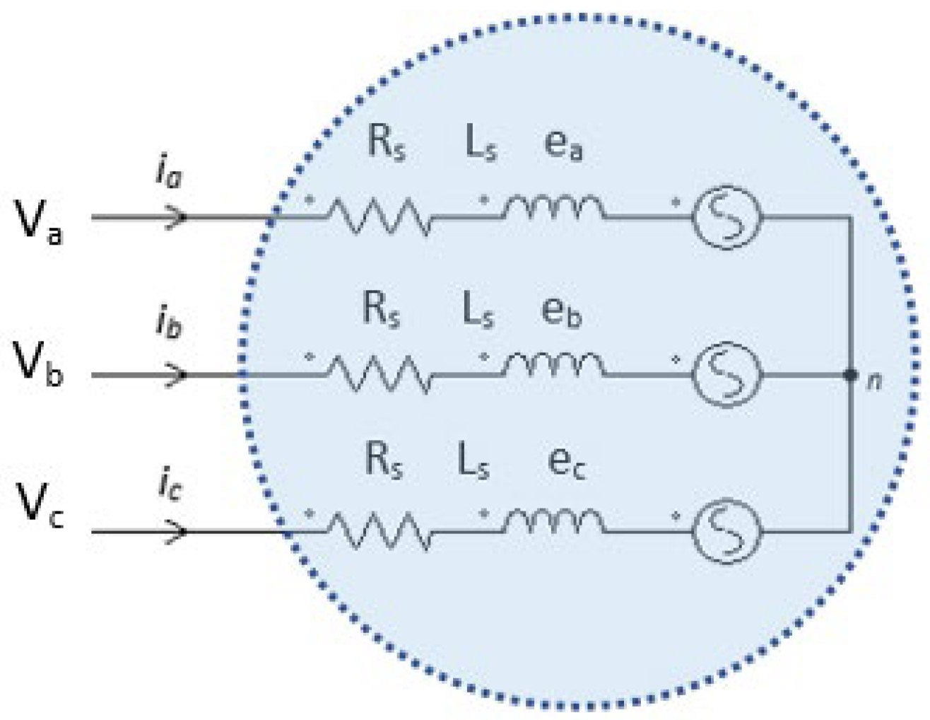
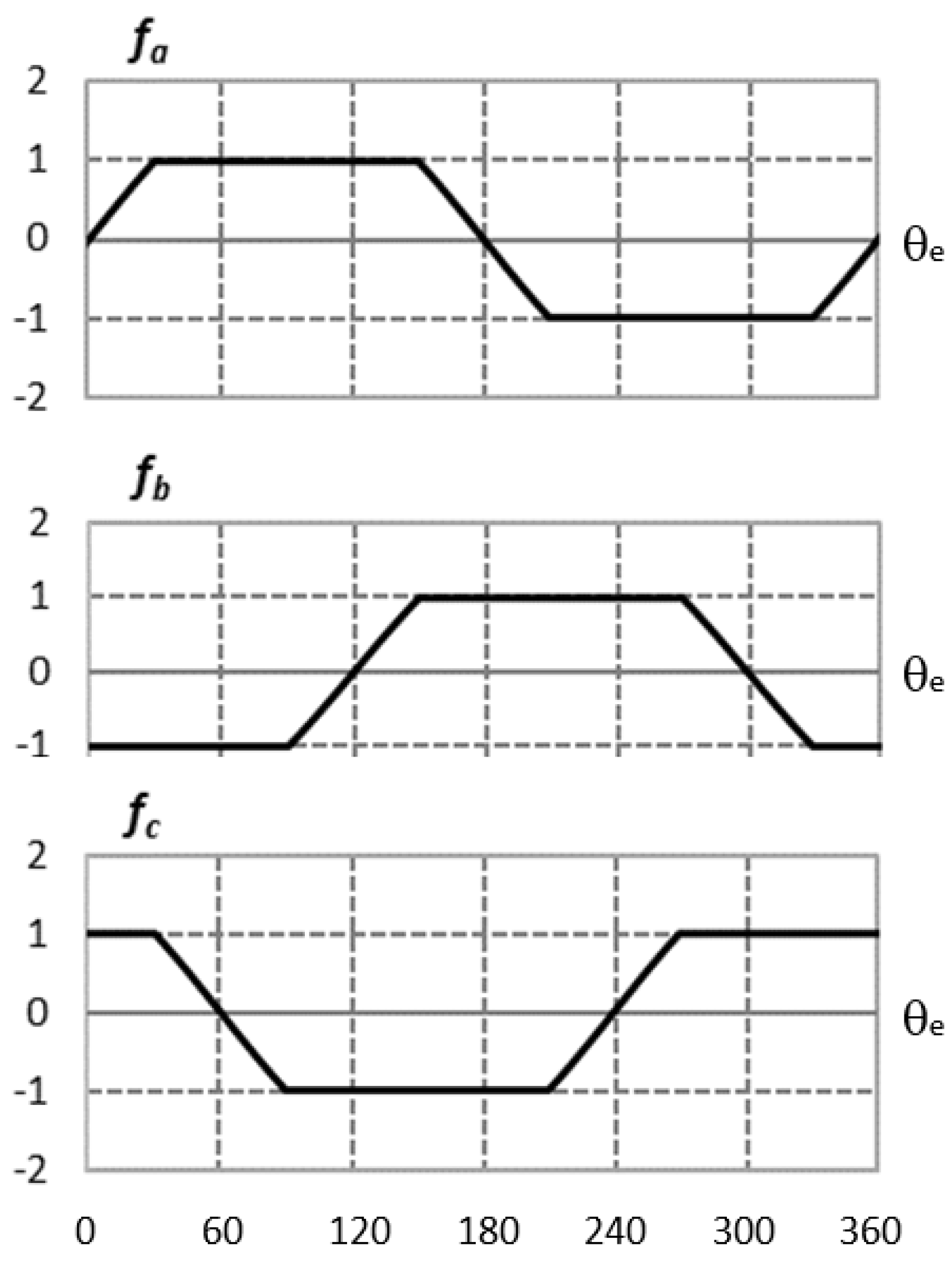
2. Mathematical Model of the BLDC Motor

The simplified equivalent circuit of the BLDC motor is shown in Figure 1, where the per-phase stator winding is represented by a resistance (R_s) and the equivalent inductance (L_s). The per-phase back-EMFs (e_an, e_bn, and e_cn) are sinusoidal waveforms in the case of a BLAC motor, but trapezoidal in the case of the BLDC. The back-EMFs are displaced 120 electrical degrees from each other. The motor is driven by a three-phase inverter, where the position of the rotor magnetic field should be detected instantaneously for proper switching commutation with the aid of three Hall sensors installed inside the BLDC motor on the stator frame [48].

In this paper, the mathematical model parameters of the BLDC motor are given using the PSIM^® package. However, the motor parameters can be identified using the methodology presented in [49].

The following set of equations can be utilized to construct the mathematical model of the BLDC motor in the case of trapezoidal EMFs. Firstly, the terminal voltages are given by Equations (1)–(3) for the three phases a, b, and c, respectively:

$$v_{an}=R_a{i}_a+\frac{d}{dt}\left(L_a{i}_a+M_{ab}{i}_b+M_{ac}{i}_c\right)+e_{an}$$

(1)

$$v_{bn}=R_b{i}_b+\frac{d}{dt}\left(L_b{i}_b+M_{ba}{i}_a+M_{bc}{i}_c\right)+e_{bn}$$

(2)

$$v_{cn}=R_c{i}_c+\frac{d}{dt}\left(L_c{i}_c+M_{ca}{i}_a+M_{cb}{i}_b\right)+e_{cn}$$

(3)

As the three-phase stator windings are symmetrical, the windings’ self-inductances are equal. Similarly, the mutual inductances are also equal. Accordingly, Relations (4), (5), and (6) are valid:

$$R_a=R_b=R_c=R_s$$

(4)

$$L_a=L_b=L_c=L$$

(5)

$$M_{ab}=M_{ba}=M_{ac}=M_{ca}=M_{bc}=M_{cb}=M$$

(6)

Substituting these values into Equations (1)–(3) yields the following relations [50,51]:

$$v_{an}=R_s{i}_a+\left(L-M\right)\frac{d}{dt}{i}_a+e_{an}$$

(7)

$$v_{bn}=R_s{i}_b+\left(L-M\right)\frac{d}{dt}{i}_b+e_{bn}$$

(8)

$$v_{cn}=R_s{i}_c+\left(L-M\right)\frac{d}{dt}{i}_c+e_{cn}$$

(9)

where L is the self-inductance, M is the mutual inductance and $(L_s=L-M)$ is the equivalent phase inductance. For trapezoidal back-EMFs, the following relations can be utilized to represent the induced EMFs in the BLDC motor:

$$e_a=K_e{\omega }_m{f}_a\left({\theta }_e\right)$$

(10)

$$e_b=K_e{\omega }_m{f}_b\left({\theta }_e\right)$$

(11)

$$e_c=K_e{\omega }_m{f}_c\left({\theta }_e\right)$$

(12)

where $K_e$ is the back-EMF constant, ${\omega }_m$ is the mechanical speed in rad/s, and $f_a\left({\theta }_e\right),f_b\left({\theta }_e\right)$ and $f_c\left({\theta }_e\right)$ are three-phase trapezoidal waveforms of unity magnitudes, as explained in Appendix A.

The electromagnetic torque developed by the BLDC motor is given by the following equation [50]:

$$T_{em}=\frac{\left(e_a{i}_a+e_b{i}_b+e_c{i}_c\right)}{{\omega }_m}$$

(13)

The electromagnetic torque produced by the BLDC motor is utilized to drive the mechanical load and overcome the mechanical friction and inertia of the motor during speed acceleration, as given by the following equation [36,50]:

$$T_{em}=T_L+J_m\frac{d{\omega }_m}{dt}+B{\omega }_m$$

(14)

By comparison, the constant current model presented in [52] can be utilized to obtain the transfer function of the BLDC motor, in a way similar to the DC motor.

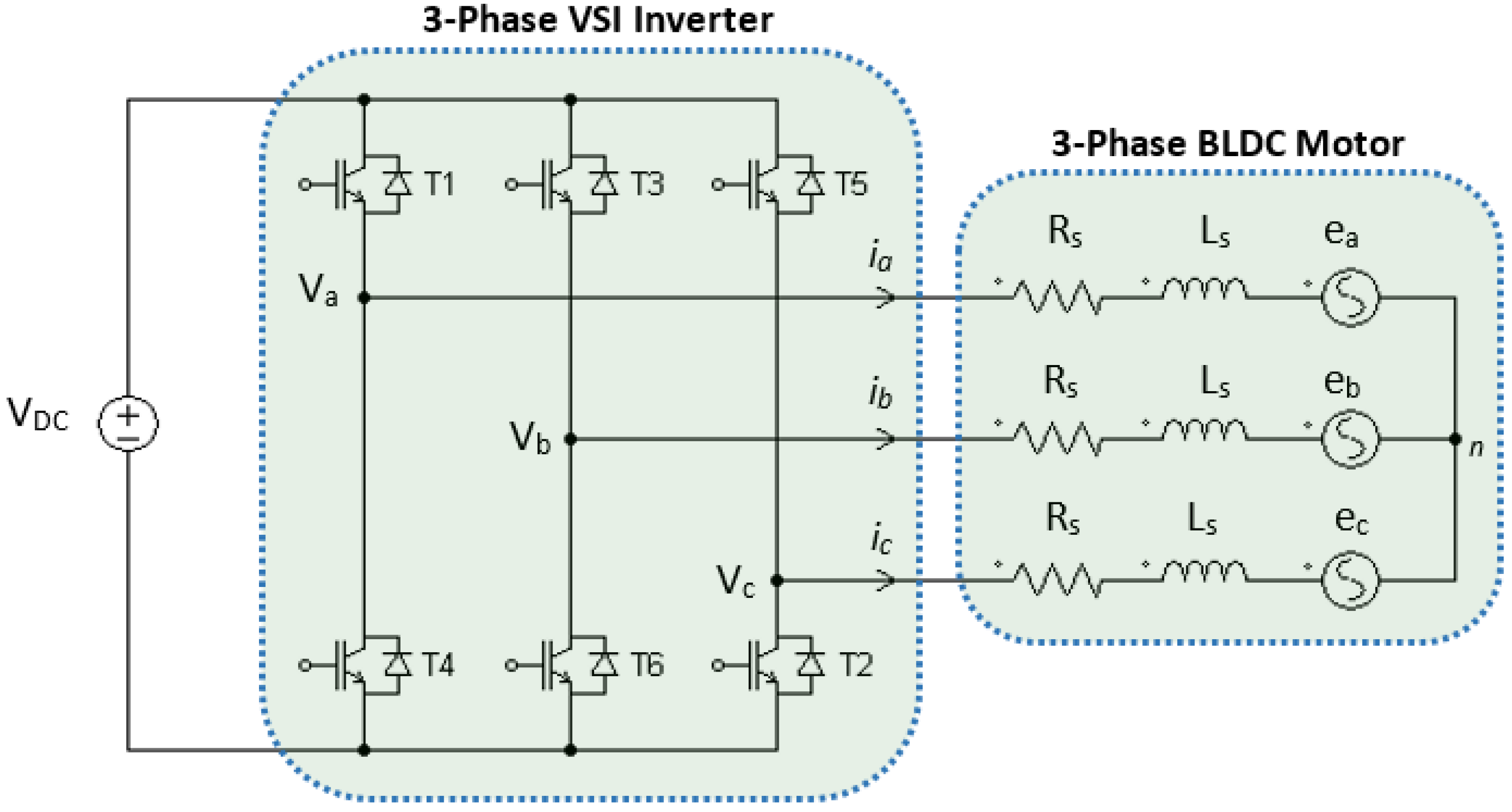
3. Description of the Three Investigated Systems

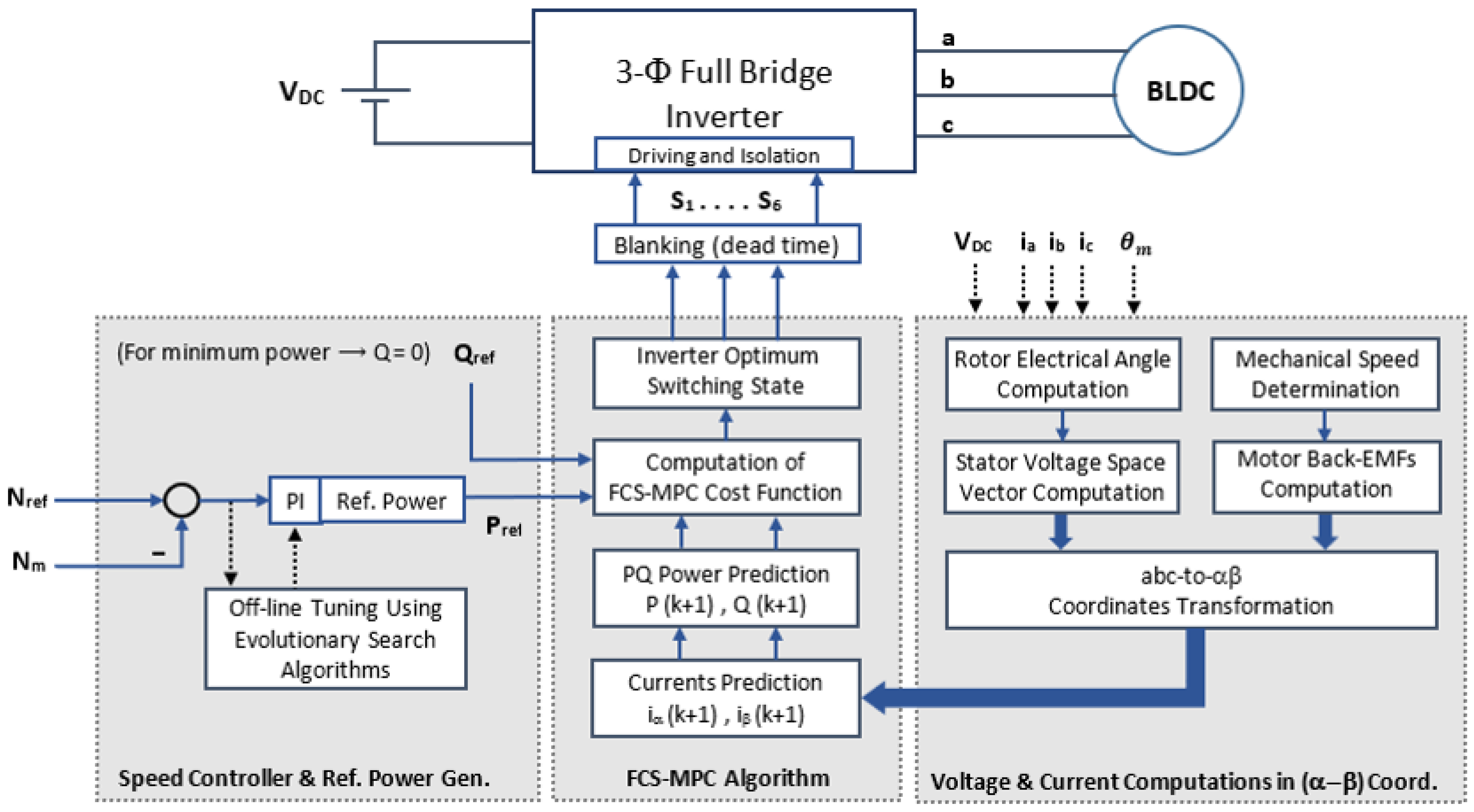
3.1. Direct Power Control Scheme (PQ FCS-MPC)

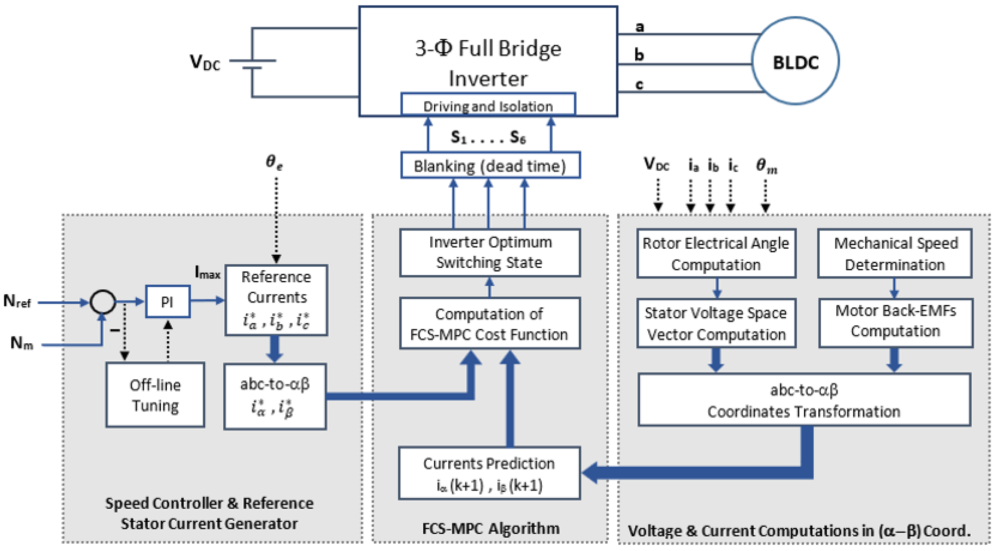
3.1.1. Block Diagram of the Direct Power Control Scheme (PQ FCS-MPC)

The block diagram of the first investigated system, the direct power control (PQ FCS-MPC) scheme, is illustrated in Figure 2. The control system has three main parts: (1) the speed control loop and reference power generation; (2) the calculations of stator, back-EMFs, stator voltage, and currents in the stationary reference frame; and (3) the FCS-MPC algorithm. The closed loop control of the BLDC motor is developed by a PI controller whose output is limited to upper and lower values. The optimum gains of the PI controller are determined off-line using evolutionary search algorithms (the tuning of PI controllers is beyond the scope of this paper). The output of the speed controller is the desired developed torque that should be produced by the BLDC motor. Then, the reference active power (P_ref) is calculated by multiplying the motor speed (N_m) with the generated reference torque (T_ref). Furthermore, the desired reactive power is set to zero to minimize the reactive power consumption. Accordingly, the BLDC motor operates at unity PF. The direct PQ FCS-MPC scheme of the BLDC motor requires determination (measurements or computations) of motor back-EMFs, stator voltages, and currents in the stationary (α–β) reference frame. These signals are determined and fed to the FCS-MPC algorithm, which regulates the active and reactive power fed to the motor in accordance with the set points (desired values). As shown in Figure 2, the FCS-MPC algorithm is composed of several blocks and functions, such as the prediction of stator currents one sample ahead, prediction of active and reactive powers one sample ahead, computation of the cost function, and selection of the optimum switching state of the voltage source inverter.

3.1.2. Prediction of Stator Currents One Sample Ahead

The FCS-MPC approach is among the techniques that control the operation of switching power converters. In the FCS-MPC technique, the future behavior of the system is predicted for a finite time frame [40]. The optimum future control action is applied to the system to satisfy a customized goal function [37]. Generally, the FCS-MPC approach results in fast transient responses and can involve many constraints in the control law [42].

Due to Equations (7)–(9), the inverter output phase voltages are written again in Equations (15)–(17):

$$v_{an}=i_a{R}_S+L_S\frac{d{i}_a}{dt}+e_{an}$$

(15)

$$v_{bn}=i_b{R}_S+L_S\frac{d{i}_b}{dt}+e_{bn}$$

(16)

$$v_{cn}=i_c{R}_S+L_S\frac{d{i}_c}{dt}+e_{cn}$$

(17)

The rates of change in the motor currents $\frac{d{i}_a}{dt}$, $\frac{d{i}_b}{dt}$, and $\frac{d{i}_c}{dt}$ are rearranged as given below:

$$\frac{d{i}_a}{dt}=\frac{1}{L_S}\left(v_{an}-e_{an}\right)-i_a\frac{R_S}{L_S}$$

(18)

$$\frac{d{i}_b}{dt}=\frac{1}{L_S}\left(v_{bn}-e_{bn}\right)-i_b\frac{R_S}{L_S}$$

(19)

$$\frac{d{i}_c}{dt}=\frac{1}{L_S}\left(v_{cn}-e_{cn}\right)-i_c\frac{R_S}{L_S}$$

(20)

Accordingly, the predicted value of the motor phase current i_a at the (k + 1)th sample is determined as follows:

$$\Delta i_a=\frac{\Delta t}{L_S}\left(v_{an}-e_{an}\right)-\Delta t i_a\frac{R_S}{L_S}$$

(21)

$$i_a^{k+1}-i_a^k=\frac{T_S}{L_S}\left(v_{an}-e_{an}\right)-T_S{i}_a^k\frac{R_S}{L_S}$$

(22)

$$i_a^{k+1}=i_a^k+\frac{T_S}{L_S}\left(v_{an}-e_{an}\right)-T_S{i}_a^k\frac{R_S}{L_S}$$

(23)

$$i_a^{k+1}=i_a^k\left(1-T_S\frac{R_S}{L_S}\right)+\frac{T_S}{L_S}\left(v_{an}-e_{an}\right)$$

(24)

where $L_s$ is the equivalent phase inductance of the motor stator winding, $R_s$ is the equivalent phase resistance of the motor stator winding, and T_S is the sampling time. Thus, the instantaneous stator currents of the other phases, i_b and i_c, at the (k + 1)th sample are predicted in a similar way:

$$i_b^{k+1}=i_b^k\left(1-T_S\frac{R_S}{L_S}\right)+\frac{T_S}{L_S}\left(v_{bn}-e_{bn}\right)$$

(25)

$$i_c^{k+1}=i_c^k\left(1-T_S\frac{R_S}{L_S}\right)+\frac{T_S}{L_S}\left(v_{cn}-e_{cn}\right)$$

(26)

From (22), (23), and (24), the stator currents of the BLDC motor sample can be predicted at the (k + 1)th sample based on the knowledge of the back-EMFs (e_an, e_bn, e_cn), inverter phase voltages (v_an, v_bn, v_cn), and stator currents i_a, i_b, and i_c at the current kth sample.

3.1.3. Computation of the Stator Voltage Space Vector

The space vector components of the stator voltage in the (α–β) frame are required for the FCS-MPC algorithm. The inverter output voltages (v_an, v_bn, v_cn) are usually measured directly by three Hall effect voltage transducers, while their (α–β) components in the stationary reference frame are calculated based on Equations (31) and (32), where the voltage space vector ${\overline{U}}_S$ is described by Equations (27) and (29) [40]:

$${\overline{U}}_S=\frac{2}{3}\left(v_{an}+a{v}_{bn}+a^2{v}_{cn}\right)$$

(27)

$$a={\mathrm{e}}^{\mathrm{j}2\pi /3};a^2={\mathrm{e}}^{\mathrm{j}4\pi /3}$$

(28)

$${\overline{U}}_S=\frac{2}{3}\left(v_{an}+e^{j2\pi /3}{v}_{bn}+e^{j4\pi /3}{v}_{cn}\right)$$

(29)

$${\overline{U}}_S=v_{\alpha }+j{v}_{\beta }$$

(30)

$$u_{\alpha }=v_{\mathrm{an}}$$

(31)

$$u_{\beta }=\frac{1}{\sqrt{3}}{v}_{\mathrm{bc}}$$

(32)

To reduce the total number of transducers and the overall cost, the motor terminal voltages can be computed (instead of measurements) based on the on-line status of the inverter switching state at the (k)th sample and the direct measurement of the inverter DC link voltage. Accordingly, only one Hall effect voltage transducer is utilized to determine the stator voltage space vector, as indicated by Equations (33)–(35).

$${\overline{U}}_S=\frac{2}{3}{V}_{DC}\left(S_1+e^{j2\pi /3}{S}_3+e^{j4\pi /3}{S}_5\right)$$

(33)

Consequently, the voltage space vector ${\overline{U}}_S$ can be resolved into two orthogonal components (U_α and U_β) in the (α–β) reference frame, where their equivalent values are calculated by (34) and (35) as given below:

$$u_{\mathsf{\alpha }}=\frac{2}{3}{V}_{DC}\left(S_1-\frac{1}{2}{S}_3-\frac{1}{2}{S}_5\right)$$

(34)

$$u_{\mathsf{\beta }}=\frac{2}{3}{V}_{DC}\left(\frac{\sqrt{3}}{2}{S}_3-\frac{\sqrt{3}}{2}{S}_5\right)$$

(35)

3.1.4. Computation of the Motor Back-EMFs in (α–β) Coordinates

For trapezoidal back-EMFs, the corresponding components of back-EMFs in the (α–β) stationary reference frame, e_α and e_β, can be calculated using Equations (36) and (37):

$$e_{\alpha }=e_{an}$$

(36)

$$e_{\beta }=\frac{1}{\sqrt{3}}{e}_{bc}$$

(37)

where the motor back-EMFs are previously described by Equations (38)–(40):

$$e_a=K_e{\omega }_m{f}_a\left({\theta }_e\right);e_b=K_e{\omega }_m{f}_b\left({\theta }_e\right);\mathrm{and}{e}_c=K_e{\omega }_m{f}_c\left({\theta }_e\right)$$

3.1.5. Prediction of Active and Reactive Power

Based on the PQ theory, the instantaneous active and reactive powers (P and Q) fed to the BLDC motor are computed using Equations (38) and (39), respectively, [34,35]:

$$P=\left(e_{\alpha }{i}_{\alpha }+e_{\beta }{i}_{\beta }\right)$$

(38)

$$Q=\left(e_{\beta }{i}_{\alpha }-e_{\alpha }{i}_{\beta }\right)$$

(39)

Transforming Equations (24)–(26) into the equivalent (α–β) components leads to the prediction of the currents i_α and i_β at the (k + 1)th sample using Equations (40) and (41):

$$i_{\alpha }^{k+1}=i_{\alpha }^k\left(1-T_S\frac{R_S}{L_S}\right)+\frac{T_S}{L_S}\left(u_{\alpha }-e_{\alpha }\right)$$

(40)

$$i_{\beta }^{k+1}=i_{\beta }^k\left(1-T_S\frac{R_S}{L_S}\right)+\frac{T_S}{L_S}\left(u_{\beta }-e_{\beta }\right)$$

(41)

where u_α and u_β are determined using either Equations (31) and (32) or by Formulas (34) and (35), while e_α and e_β are determined using Equations (36) and (37). Thus, from Equations (38), (39), (40), and (41), the instantaneous active and reactive powers fed to the BLDC motor are predicted at the (k + 1)th sample using Equations (42) and (43):

$$P^{k+1}=\left(e_{\alpha }^{k+1}{i}_{\alpha }^{k+1}+e_{\beta }^{k+1}{i}_{\beta }^{k+1}\right)$$

(42)

$$Q^{k+1}=\left(e_{\beta }^{k+1}{i}_{\alpha }^{k+1}-e_{\alpha }^{k+1}{i}_{\beta }^{k+1}\right)$$

(43)

Since the back-EMFs have relatively slow variation compared to the sampling and switching frequencies, the back-EMF components e_α and e_β can be considered constant during the sampling period, i.e., ($e_{\alpha }^{k+1}=e_{\alpha }^k$) and ($e_{\beta }^{k+1}=e_{\beta }^k$) [41,42].

3.1.6. Formulation of the Cost Function

The cost function of the direct PQ FCS-MPC algorithm is formulated to account for active and reactive powers fed to the BLDC motor as given by Equation (44):

$$J_{pq}={\left(P_{ref}-P^{k+1}\right)}^2+{\left(Q_{ref}-Q^{k+1}\right)}^2$$

(44)

where $P_{ref}$ and $Q_{ref}$ are the reference (desired) values of the active and reactive powers to be fed to the BLDC motor from the DC source through the 3-ΦVSI inverter. Due to Equation (44), the first term of the cost function aims to minimize the active power ripple, whereas the second term aims to minimize the reactive power ripple.

Both terms have the same degree of importance. For minimum reactive power fed to the motor, its reference value is set to zero $(Q_{ref}=0)$. In the direct PQ FCS-MPC approach, the cost function J_pq in Equation (44) is computed for all inverter switching states. Then, the switching state number i, which results in the lowest possible value of the cost function (J_i = J_{pq min}), is selected and considered as the optimum state to be applied to the transistors of the VSI during the next sample. In this manner, the cost function is instantaneously optimized for every sampling period, and the corresponding optimum switching state is determined and applied to the VSI inverter, driving the BLDC motor to the desired operating point.

3.2. Stator Current Controlled Scheme (CC FCS-MPC)

3.2.1. Block Diagram of the Stator Current Controlled Scheme (CC FCS-MPC)

The block diagram of the second investigated system, the current controlled FCS-MPC scheme of the BLDC motor, is illustrated in Figure 3. The control system is composed of three main parts: (1) the speed control loop and generation of the reference amplitude of stator currents; (2) the computations of stator voltage, currents, and back-EMFs in the stationary reference frame; and (3) the FCS-MPC algorithm. The closed loop control of the BLDC motor is developed by a PI controller with limited output. The optimum gains of the controller’s parameters are determined off-line using evolutionary search algorithms (the tuning of PI parameters is beyond the scope of this paper). The output of the speed controller represents the amplitude (peak value) of the stator current to satisfy the motor operation.

The reference quasi-square waves of the stator currents are generated with the aid of the electrical angle, computed from the knowledge of the mechanical rotor position and the number of poles of the BLDC motor, as given by Equation (45).

$${\theta }_e=\frac{P}{2}{\theta }_m$$

(45)

where P is the number of rotor poles and θ_m is the rotor mechanical position. The prediction of the stator currents one sample ahead is similar to that explained in Section 3.1.2. In addition, the computation of the stator voltage space vector and the computation of the motor back-EMFs in (α–β) coordinates are similar to those presented in Section 3.1.3 and Section 3.1.4, respectively. Thus, these equations and their explanations are not repeated.

3.2.2. Formulation of the Cost Function

The cost function of the current-controlled FCS-MPC algorithm is formulated in Equation (46). The cost function aims to minimize the absolute error between the reference and actual stator current components in (α–β) coordinates.

$$J_{cc}=\left|i_{\alpha }^{*}-i_{\alpha }\right|+\left|i_{\beta }^{*}-i_{\beta }\right|$$

(46)

where $i_{\alpha }^{*}$ and $i_{\beta }^{*}$ are the reference (desired) values of the stator current components in (α–β) coordinates, and $i_{\alpha }$ and $i_{\beta }$ are the corresponding actual values. In the current controlled FCS-MPC approach, the cost function J_cc in Equation (46) is computed for all inverter switching states. Then, the switching state number i, which results in the lowest possible value of the cost function $\left(J_i=J_{ccmin}\right)$, is selected to be the optimum state that should be applied to the transistors of the VSI during the next sample. Thus, the cost function is instantaneously optimized for every sampling period, and the corresponding optimum switching state is determined and applied to the inverter, driving the BLDC motor to the desired operating point.

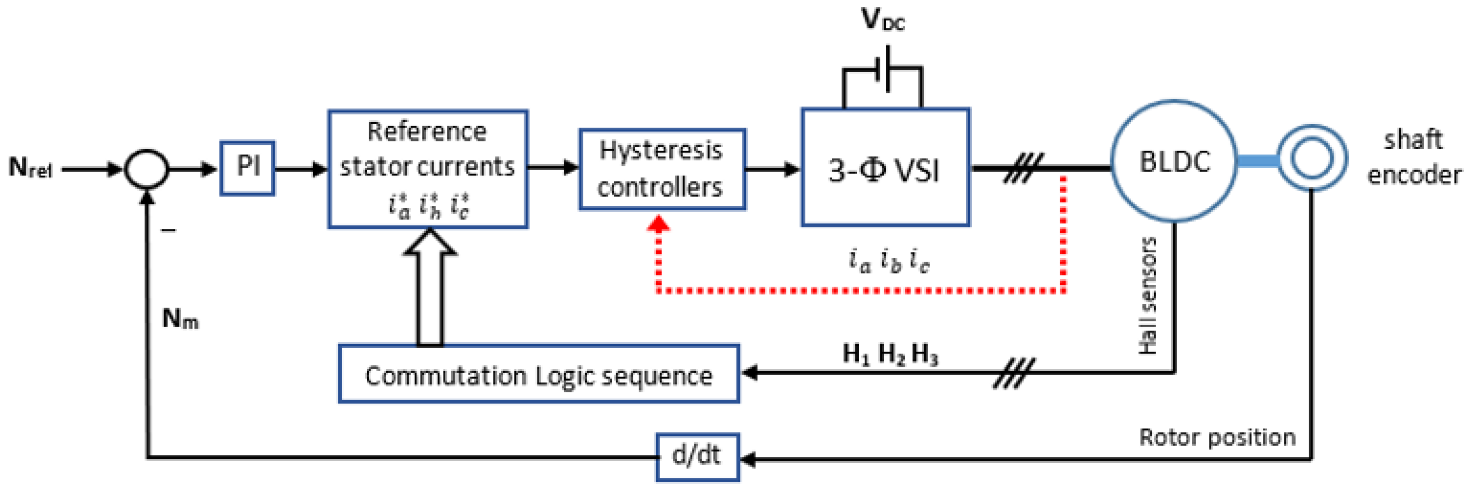
3.3. Stator Current Controlled Scheme with Hysteresis Current Controllers (Hysteresis CC)

The third investigated scheme of the BLDC motor is illustrated in Figure 4. In this scheme, the motor speed is regulated by a PI-type speed controller. The output of the speed controller represents the amplitude of the reference (desired) 3-Φ stator currents (I_max), whereas the waveforms of the reference stator currents (quasi-square waves of 120° mode) are generated with the aid of a commutation logic decoder, which converts the status of the three Hall sensors into 3-Φ signals displaced 120 electrical degrees from each other. The stator currents are controlled by three hysteresis current controllers with a certain tolerance band. The outputs of the ON–OFF current controllers are employed to generate the switching signals of the transistors of the 3-Φ VSI inverter.

4. Selected Simulation Results of the Investigated Systems

The three studied systems of the BLDC motor drive were modeled and investigated in the PSIM^® software. The simulation parameters are summarized in

Table 1. Simulation parameters.

Parameter	Value
Simulation Platform	PSIM
MPC Sampling time TS	10–20 μs
Motor phase resistance RS	10 Ω
Equivalent phase inductance LS	6 mH
Back-EMF constant	0.2 V/rpm
Motor poles	8
Moment of inertia	0.0005 kgm2

. In this section, some simulation results are presented and discussed. The illustrated results are categorized into two main groups: (1) the steady state performance of the elaborated schemes, and (2) the transient response of the investigated systems. Both result groups include quantitative assessments. In the first group of results, various steady state waveforms are illustrated for qualitative comparison. The corresponding harmonic spectra are also addressed graphically. In the second group, the transient responses of the investigated systems under both step variations in the reference speed and step changes in the load are presented.

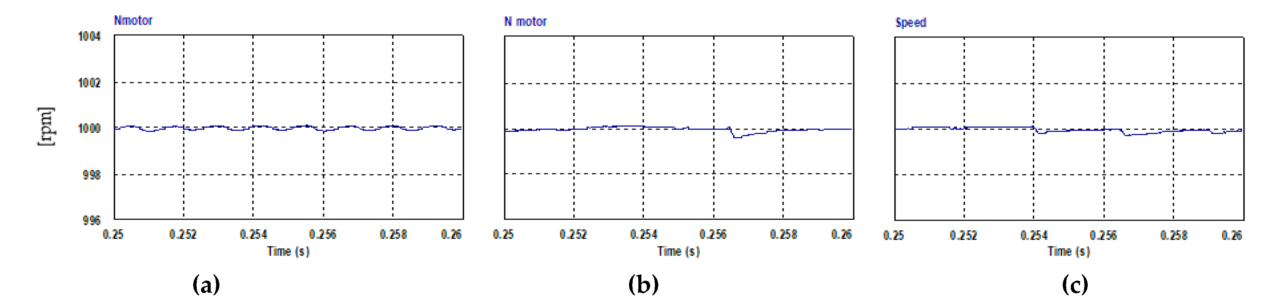
4.1. Steady State Performance

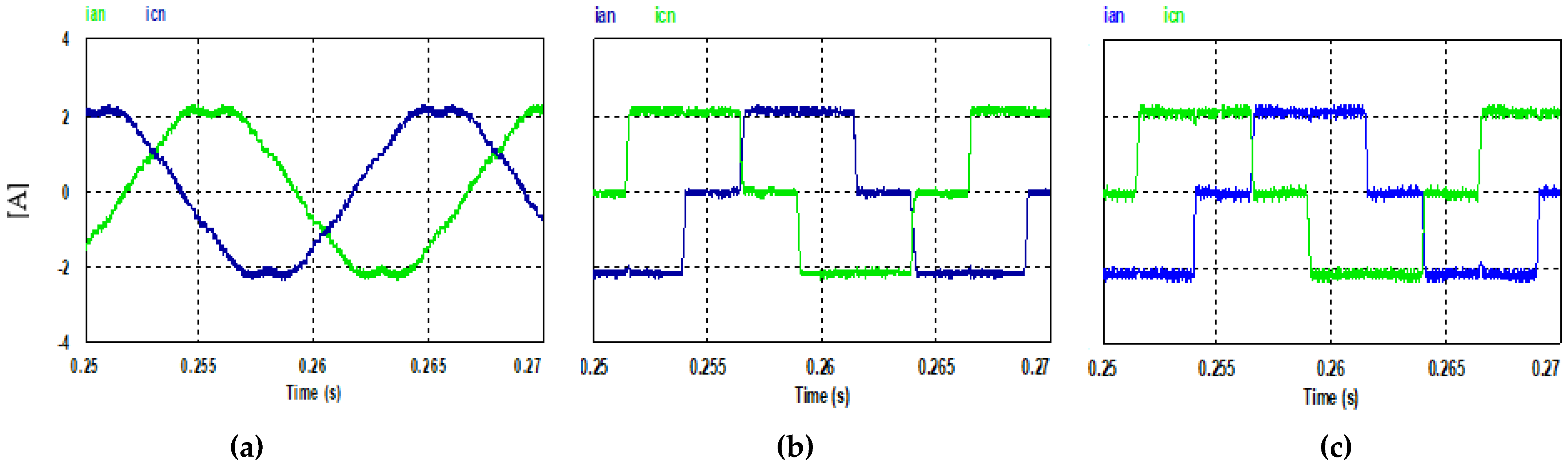
4.1.1. Time-Domain Waveforms

The three systems were operated under the same conditions, where the reference speed was set to 1000 RPM and the load torque was set to 2.5 N.m.

The steady state waveforms of the mechanical speed, stator currents, electromagnetic torque developed by the motor, active power consumed by the motor, reactive power supplied to the motor, stator current components in the (α–β) reference frame, back-EMF, and stator current of the same phase are illustrated in Figure 5, Figure 6, Figure 7, Figure 8, Figure 9, Figure 10 and Figure 11, respectively. The obtained results indicate that the motor mechanical speed was well controlled to the desired value, with negligible ripples in all three systems. The stator current was of better quality with the direct PQ FCS-MPC than with the other schemes. Moreover, the lowest peak-to-peak ripple torque was achieved with the direct PQ FCS-MPC scheme. The peak-to-peak ripple in active and reactive power were also at minimum values in the case of the direct PQ FCS-MPC scheme.

The other two schemes, the CC FCS-MPC scheme and the current control with hysteresis current controllers, resulted in low frequency pulsations in torque and active power waveforms. In addition, the reactive power had high ripples compared to the direct PQ FCS-MPC scheme. The worst quality of stator currents was obtained with the scheme using hysteresis current controllers. The quantitative assessment is presented in detail in

Table 2. Quantitative assessment of steady state performance: (N_ref = 1000 rpm; T_L = 2.5 N.m).

Item	Parameter			Value
				DPC FCS-MPC	CC FCS-MPC	Hysteresis CC
Motor Speed [RPM]	Reference Value		Nref	1000	1000	1000
	Worst values	Max.	Nmax	1000.16	1000.22	1000.19
		Min.	Nmin	999.84	999.53	999.72
	Average		Navg	1000	999.99	999.99
	% Speed Error		100 × (Nmax − Nmin)/Nref	0.032	0.069	0.047
Developed Torque [N.m]	Average Torque		Tag	2.58	2.69	2.70
	Worst values	Max.	Tmax	2.72	2.98	2.89
		Min.	Tmin	2.44	1.82	2.27
	% Peak-Peak Ripple		100 × (Tmax − Tmin)/Tavg	10.85	43.12	22.96
Active Power [W]	Average Power		Pavg	270.51	282.39	282.86
	Worst values	Max.	Pmax	285.29	313.03	303.33
		Min.	Pmin	255.68	190.32	238.18
	% Peak-Peak ripple		100 × (Pmax − Pmin)/Pavg	10.94	43.45	23.03
Reactive Power [VAR]	Average Value		QAVG	2.39	8.21	12.33
	Worst Values	Max.	Qmax	19.93	171.56	183.94
		Min.	Qmin	−14.44	−151.26	−158.50
	Peak-Peak Ripple		ΔQ = (Qmax − Qmin)	34.37	322.82	342.44
Stator Current [A]	RMS Value		Irms	1.586	1.721	1.733
	Peak of 1st Harmonic		I1 peak	1.869	1.937	1.938
	% Total Harm. Dist.		THD	9.09	28.98	30.60

. According to the results obtained, the direct PQ FCS-MPC scheme resulted in the relatively best steady state performance.

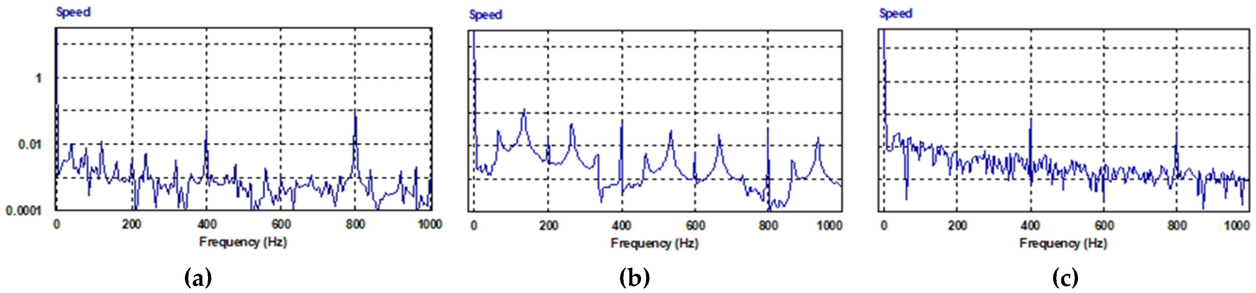
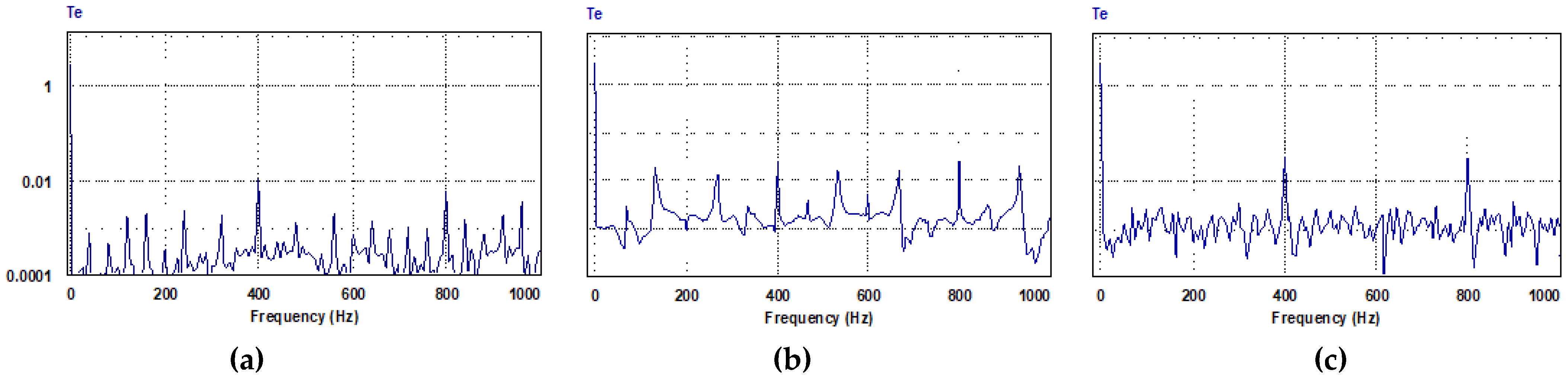
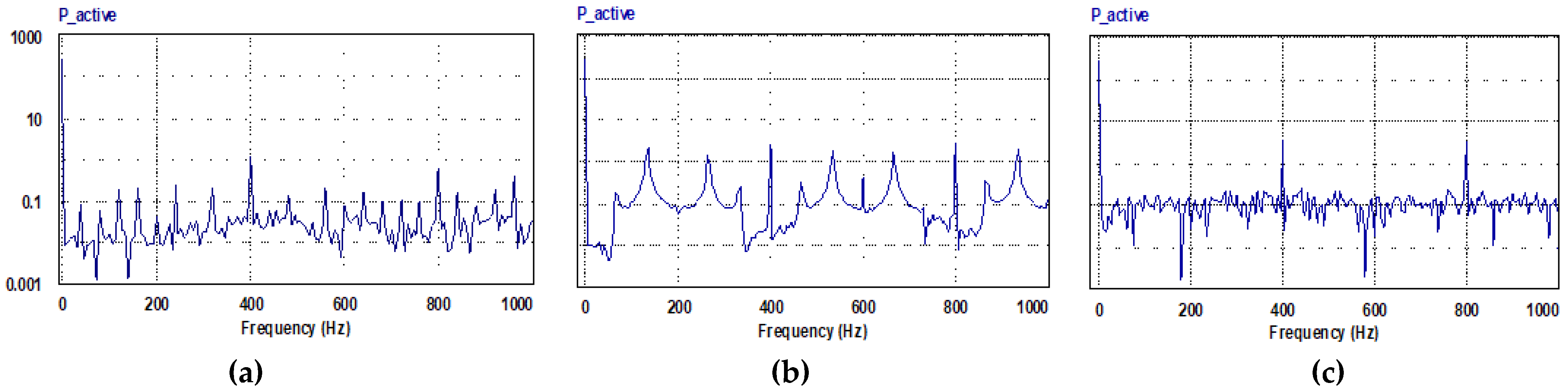
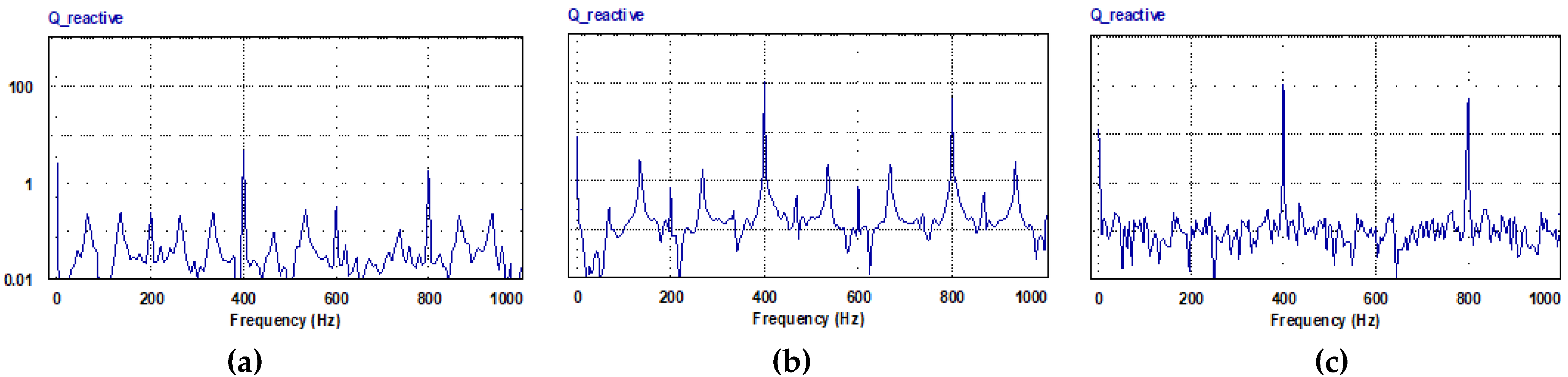
4.1.2. Harmonic Spectra

The harmonic spectra corresponding to the previously sketched waveforms in Figure 5, Figure 6, Figure 7, Figure 8 and Figure 9 were determined and are sketched in Figure 10, Figure 11, Figure 12, Figure 13 and Figure 14. In Figure 10, the harmonic spectra of the motor speed for the three schemes are presented. The results indicate that the dominant low order harmonics are the 6th and 12th components. However, their magnitudes are negligible (<0.06% in the worst case, the hysteresis current controller) (see quantitative assessment results of

Table 3. Quantitative assessment of harmonic spectra: (N_ref = 1000 rpm; T_L = 2.5 N.m).

Item	Parameter		Value
			DPC FCS-MPC	CC FCS-MPC	Hysteresis CC
Motor Speed [rpm]	Reference Value	Nref	1000	1000	1000
	Amplitudes of the worst low order harmonics	2nd order	---	0.135	---
		4th	---	0.0466	---
		6th order	0.0256	0.0468	0.064
Line-Line voltage [V]	Amplitude of 1st harmonic	1st order	214.23	215.88	210.91
	Amplitudes of the worst low order harmonics	5th order	32.71	23.73	21.12
		7th order	26.06	17.48	17.98
		11th order	12.97	23.84	27.89
Developed Torque [N.m]	Amplitudes of the worst low order harmonics	2nd order	---	0.02	---
		4th order	---	0.014	---
		6th order	0.0105	0.027	0.0348
		12th order	0.0062	0.025	0.0317
Active Power [W]	Amplitudes of the worst low order harmonics	2nd order	---	2.21	---
		4th order	---	1.43	---
		6th order	1.10	2.87	3.64
		8th order	---	1.84	---
		12th order	0.632	2.66	3.32
Reactive Power [VAR]	Amplitudes of the worst low order harmonics	6th order	4.37	106.41	110.03
		12th order	1.25	49.03	51.69
		18th order	0.587	32.10	33.81
Stator Current [A]	RMS Value	Irms	1.586	1.721	1.733
	Amplitude of 1st harmonic	I1peak	1.869	1.937	1.938
	% Total Harmonic Distor.	THD	9.09	28.98	30.60
	Amplitudes of the worst low order harmonics	5th order	0.050	0.392	0.40
		7th order	0.069	0.268	0.28
		11th order	0.0058	0.175	0.186

). The harmonic spectra of the stator current (Figure 11) had low order harmonics (5th, 7th, and 11th) in all systems. However, the direct PQ FCS-MPC scheme had the best harmonic content compared to the other schemes; the THD of the stator current was 9%, and it reached 30% in the hysteresis current controller scheme.

Furthermore, the harmonic spectra of the electromagnetic signal of Figure 12 have dominant low order harmonics (6th and 12th order components). At the same time, in the CC FCS-MPC scheme, second order harmonics also exist.

In addition, the active power waveforms of Figure 13 have low order harmonics (6th and 12th) that do not exceed 3.6% in the worst case (hysteresis current controller scheme). However, the CC FCS-MPC scheme resulted in the worst harmonic content in terms of the existence of second order harmonics in the active power waveforms, as indicated in Table 3. Moreover, the harmonic spectra of the reactive power shown in Figure 14 indicate that there are low order harmonics at orders 6th and 12th. The worst values of the low order harmonics were obtained by the CC FCS-MPC scheme followed by the hysteresis current controller scheme.

4.1.3. Quantitative Analysis of the Steady State Results

The quantitative analysis of the steady state performance of the BLDC motor drive was conducted for the three elaborated schemes. The results are presented in Table 2. The results indicate that the direct PQ FCS-MPC scheme achieved the relatively best performance among the examined schemes in terms of the lowest ripples in mechanical speed, developed torque, active power, reactive power, and stator current waveforms. In addition, the quantitative analysis of the corresponding harmonic spectra summarized in Table 3 demonstrates the superiority of the direct PQ FCS-MPC scheme over the other schemes in terms of the minimum magnitudes of undesired low order harmonics and the best harmonic content in the investigated frequency range.

4.2. Transient Response

The transient response of the three elaborated BLDC systems were investigated for two different cases. The first is the transient response of the BLDC motor when it is subjected to a step change in the desired (reference) speed signal (from −1000 rpm to + 1000 rpm). The second investigated case is the BLDC motor transient performance for a step change in the mechanical load. In each case, time domain waveforms are plotted for the three investigated schemes. In addition, qualitative analysis was undertaken on the obtained results. The results are summarized in

Table 4. Quantitative assessment of transient performance.

Mode of Operation	Parameter	Value
		DPC FCS-MPC	CC FCS-MPC	Hysteresis CC
Step change in mechanical load (TLoad = 0 → 2.5 N·m) (No =1000 rpm)	Load rejection time [ms]	35	31	32
	Max dip in speed [rpm]	19	21.1	21
	Percentage of speed dip [%]	1.91	2.11	2.1
Step change in reference speed (−1000 → 1000 RPM)	Settling time [ms]	32.5	40.4	39.9
	Peak overshoot [rpm]	2	14.3	6.2

.

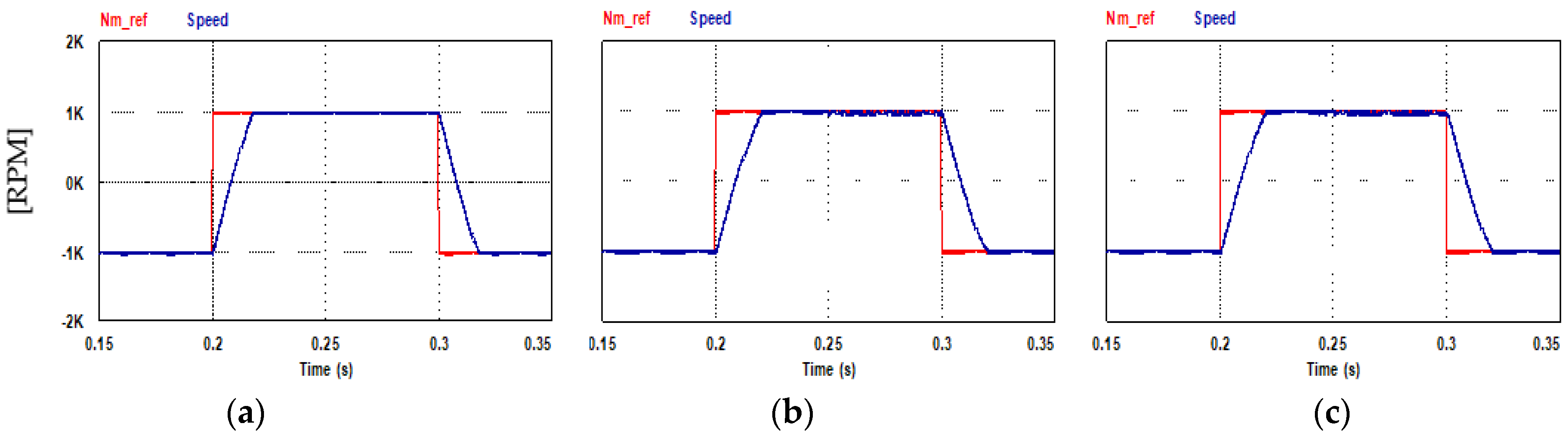
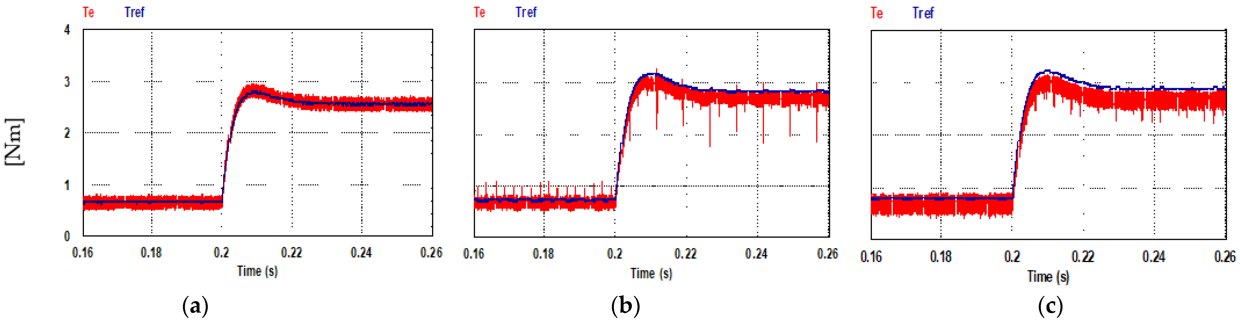
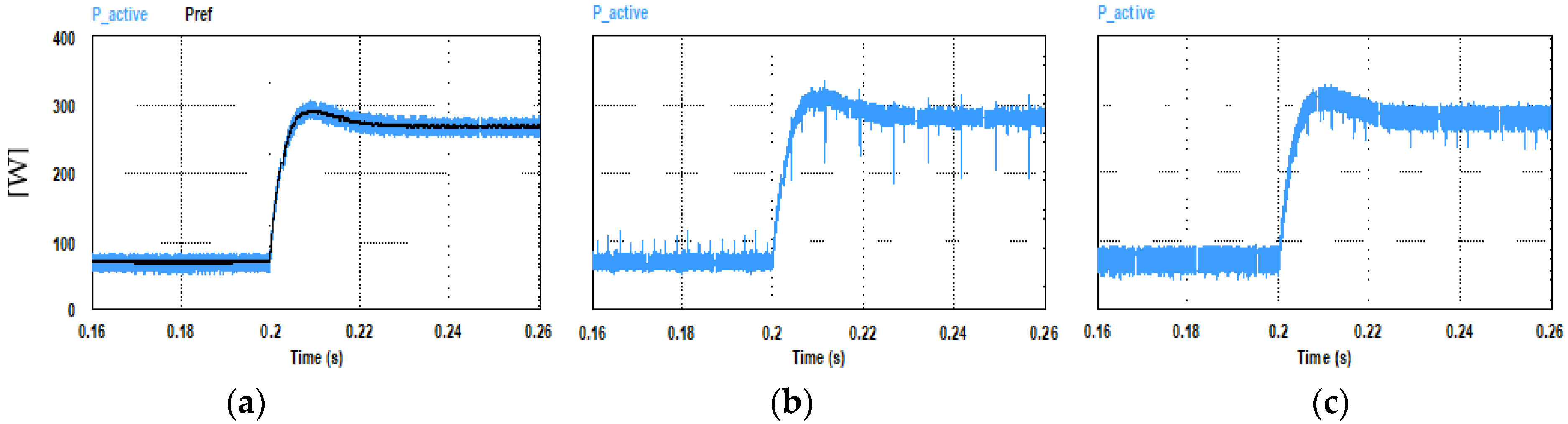
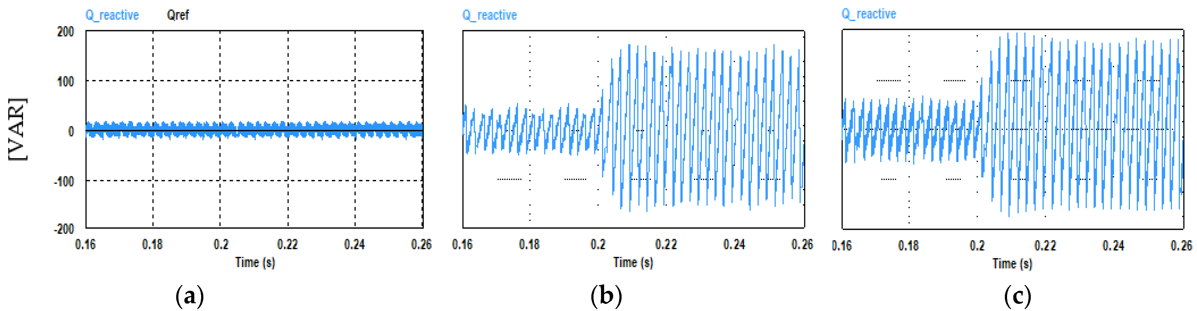
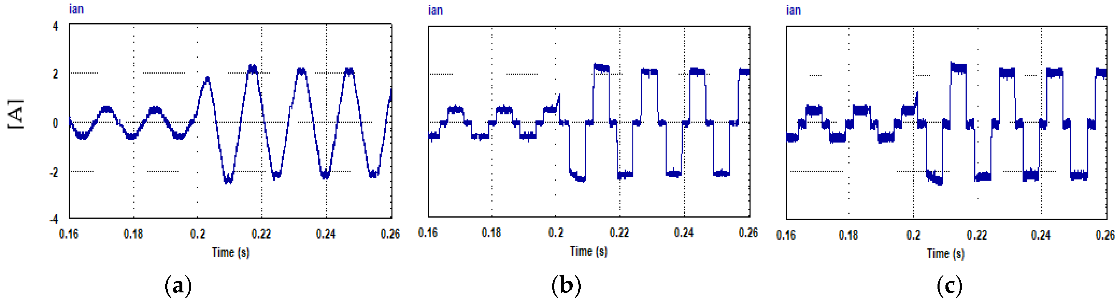
4.2.1. Step Change in the Reference Signal

As shown in Figure 15, the three investigated systems succeeded in controlling the motor speed to the set point. When the reference speed signal experienced a step change from −1000 rpm to +1000 rpm, the settling time was between 32.5 and 40.4 ms for the direct PQ FCS-MPC scheme and the CC FCS-MPC scheme, respectively. The current control scheme with the hysteresis current controller resulted in a settling time of 39.9 ms (see Table 4). The best peak overshoot was achieved with the direct PQ FCS-MPC scheme: 2 rpm (0.2%); whereas the worst peak overshoot was produced with the CC FCS-MPC scheme: 14.3 rpm (1.43%) (see Table 4).

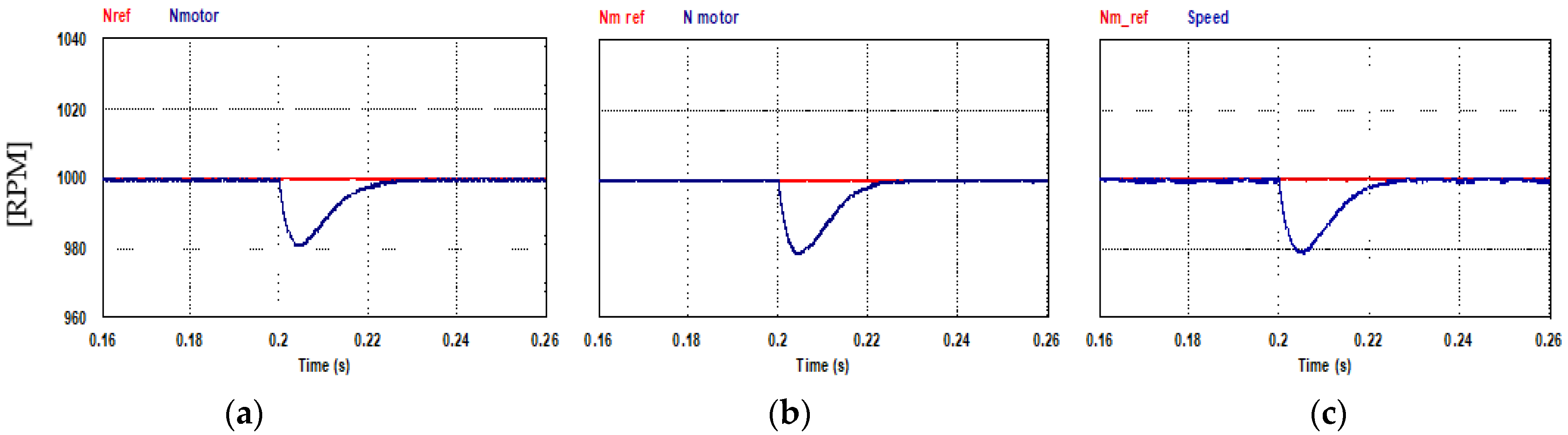
4.2.2. Sudden Load Variation (Step Change)

As illustrated in Figure 16, the motor was subjected to a sudden load change (step change) at time (t = 0.2 s). The three BLDC systems succeeded in returning the speed to the set point (1000 rpm); this occurred after approximately 35 ms in the case of the direct PQ FCS-MPC scheme, 31 ms in the case of the CC FCS-MPC scheme, and 32 ms in the case of the hysteresis current controller scheme. However, the dip speed was between 19 and 21.1 rpm in the case of the direct PQ FCS-MPC and CC FCS-MPC schemes, respectively. In the case of the hysteresis current controller, the dip speed was 21 rpm. The corresponding waveforms for the electromagnetic torque, active power, reactive power, and stator currents are presented in Figure 17, Figure 18, Figure 19 and Figure 20, respectively.

In Figure 17, it can be observed that the direct PQ FCS-MPC scheme resulted in minimum peak-to-peak ripples in the torque waveform, whereas the CC FCS-MPC scheme produced the worst waveform for the electromagnetic torque, with low frequency pulsations superimposed on the electromagnetic waveform. Similarly, the resultant waveforms of the active power consumed by the BLDC motor are plotted in Figure 18. The highest quality waveform was produced by the direct PQ FCS-MPC scheme, the power pulsation was produced by the CC FCS-MPC scheme, and the worst peak-to-to peak ripple was produced by the hysteresis current control scheme.

One of the noticeable differences between the three systems is the resultant waveform of reactive power fed to the motor as depicted in Figure 19. The best waveform obtained, with minimum possible peak-to-peak ripple, was achieved with the direct PQ FCS-MPC scheme, whereas the worst peak-peak ripple was obtained with the hysteresis current controllers scheme followed by the CC FCS-MPC scheme.

The resultant waveforms of the stator currents are plotted in Figure 20. The highest quality waveform was achieved with the direct PQ FCS-MPC scheme, whereas the lowest quality waveform was observed in the case of the hysteresis current control scheme.

4.2.3. Quantitative Analysis of the Transient Response

The quantitative analysis of the transient response of the BLDC motor drive with the elaborated schemes is summarized in Table 4.

5. Conclusions

In this paper, the performance of the BLDC motor drive trapezoidal EMFs was studied and assessed under three different control schemes. The first scheme investigated was the direct active and reactive power control using the FCS-MPC approach. This scheme provided a decoupled control of both active and reactive power fed to the motor.

The second scheme investigated was the stator current control using the FCS-MPC approach. In this scheme, the stator current components in the (α–β) coordinates were directly controlled using a finite control set model predictive controller. In the third scheme, however, the stator currents were controlled using hysteresis current controllers. The study included both steady state and transient performances. Furthermore, qualitative and quantitative analyses of the obtained results were performed.

The obtained results indicate that the three schemes can successfully operate the BLDC motor at the desired operating point. However, the direct PQ FCS-MPC scheme exhibited superior performance, especially at the steady state in terms of minimum torque ripple, minimum active and reactive power ripple, and minimum THD of the stator current, where the percentage of the peak-to-peak torque ripple did not exceed 11% of the average value, whereas, in the other schemes, this value was between 22% and 43%.

Moreover, the resultant percentage of the peak-to-peak active power ripple did not exceed 11% of the average value, whereas in the other schemes, this value was between 23% and 43%. The resultant reactive power ripple was only 10% of the corresponding values achieved with the other systems. The resultant THD of the stator current was 9%, which is 30% of the corresponding value obtained with the other schemes. Moreover, the minimum peak overshoot of 2 rpm (0.2% of the reference speed) was achieved with the DPC scheme, whereas, in other schemes, 14 rpm was reached (1.4% of the reference speed).

Furthermore, the current controlled FCS-MPC scheme produced undesired low frequency pulsations in the torque and active power waveforms with a relatively higher value of the THD of the stator current. Although the third scheme, stator current control with hysteresis current controllers, did not contribute a noticeably better performance at steady state, its cost–performance relation makes it an economic choice for low-cost BLDC drives with satisfactory performance.

References

1. Jin, H.; Liu, G.; Li, H.; Chen, B.; Zhang, H. A Fast Commutation Error Correction Method for Sensorless BLDC Motor Considering Rapidly Varying Rotor Speed. IEEE Trans. Ind. Electron. 2022, 69, 3938–3947. [Google Scholar] [CrossRef]
2. Jin, H.; Liu, G.; Zheng, S. Commutation Error Closed-Loop Correction Method for Sensorless BLDC Motor Using Hardware-Based Floating Phase Back-EMF Integration. IEEE Trans. Ind. Inform. 2022, 18, 3978–3986. [Google Scholar] [CrossRef]
3. Chen, S.; Zhou, X.; Bai, G.; Wang, K.; Zhu, L. Adaptive Commutation Error Compensation Strategy Based on a Flux Linkage Function for Sensorless Brushless DC Motor Drives in a Wide Speed Range. IEEE Trans. Power Electron. 2018, 33, 3752–3764. [Google Scholar] [CrossRef]
4. Zhao, D.; Wang, X.; Tan, B.; Xu, L.; Yuan, C.; Huangfu, Y. Fast Commutation Error Compensation for BLDC Motors Based on Virtual Neutral Voltage. IEEE Trans. Power Electron. 2021, 36, 1259–1263. [Google Scholar] [CrossRef]
5. Lee, Y. A New Method to Minimize Overall Torque Ripple in the Presence of Phase Current Shift Error for Three-Phase BLDC Motor Drive. Can. J. Electr. Comput. Eng. 2019, 42, 225–231. [Google Scholar] [CrossRef]
6. Zhang, H.; Li, H. Fast Commutation Error Compensation Method of Sensorless Control for MSCMG BLDC Motor with Nonideal Back EMF. IEEE Trans. Power Electron. 2021, 36, 8044–8054. [Google Scholar] [CrossRef]
7. Jin, H.; Liu, G.; Li, H.; Zhang, H. Closed-Loop Compensation Strategy of Commutation Error for Sensorless Brushless DC Motors with Nonideal Asymmetric Back-EMFs. IEEE Trans. Power Electron. 2021, 36, 11835–11846. [Google Scholar] [CrossRef]
8. Zhang, H.; Liu, G.; Zhou, X.; Zheng, S. High-Precision Sensorless Optimal Commutation Deviation Correction Strategy of BLDC Motor with Asymmetric Back EMF. IEEE Trans. Ind. Inform. 2021, 17, 5250–5259. [Google Scholar] [CrossRef]
9. Chen, S.; Sun, W.; Wang, K.; Liu, G.; Zhu, L. Sensorless High-Precision Position Correction Strategy for a 100 kW@20 000 r/min BLDC Motor with Low Stator Inductance. IEEE Trans. Ind. Inform. 2018, 14, 4288–4299. [Google Scholar] [CrossRef]
10. Wang, L.; Zhu, Z.Q.; Bin, H.; Gong, L. A Commutation Error Compensation Strategy for High-Speed Brushless DC Drive Based on Adaline Filter. IEEE Trans. Ind. Electron. 2021, 68, 3728–3738. [Google Scholar] [CrossRef]
11. Li, Y.; Song, X.; Zhou, X.; Huang, Z.; Zheng, S. A Sensorless Commutation Error Correction Method for High-Speed BLDC Motors Based on Phase Current Integration. IEEE Trans. Ind. Inform. 2020, 16, 328–338. [Google Scholar] [CrossRef]
12. Ebadpour, M.; Amiri, N.; Jatskevich, J. Fast Fault-Tolerant Control for Improved Dynamic Performance of Hall-Sensor-Controlled Brushless DC Motor Drives. IEEE Trans. Power Electron. 2021, 36, 14051–14061. [Google Scholar] [CrossRef]
13. Yang, L.; Zhu, Z.Q.; Gong, L.; Bin, H. PWM Switching Delay Correction Method for High-Speed Brushless DC Drives. IEEE Access 2021, 9, 81717–81727. [Google Scholar] [CrossRef]
14. Gu, C.; Wang, X.; Shi, X.; Deng, Z. A PLL-Based Novel Commutation Correction Strategy for a High-Speed Brushless DC Motor Sensorless Drive System. IEEE Trans. Ind. Electron. 2018, 65, 3752–3762. [Google Scholar] [CrossRef]
15. Kolano, K. Improved Sensor Control Method for BLDC Motors. IEEE Access 2019, 7, 186158–186166. [Google Scholar] [CrossRef]
16. Park, J.S.; Lee, K.-D. Online Advanced Angle Adjustment Method for Sinusoidal BLDC Motors with Misaligned Hall Sensors. IEEE Trans. Power Electron. 2017, 32, 8247–8253. [Google Scholar] [CrossRef]
17. Aladsani, A.S.; AlSharidah, M.E.; Beik, O. BLDC Motor Drives: A Single Hall Sensor Method and a 160° Commutation Strategy. IEEE Trans. Energy Convers. 2021, 36, 2025–2035. [Google Scholar] [CrossRef]
18. Bae, J.; Lee, D.-H. Position Control of a Rail Guided Mover Using a Low-Cost BLDC Motor. IEEE Trans. Ind. Appl. 2018, 54, 2392–2399. [Google Scholar] [CrossRef]
19. Carey, K.D.; Zimmerman, N.; Ababei, C. Hybrid field oriented and direct torque control for sensorless BLDC motors used in aerial drones. IET Power Electron. 2019, 12, 438–449. [Google Scholar] [CrossRef] [Green Version]
20. Khazaee, A.; Zarchi, H.A.; Markadeh, G.A.; Hesar, H.M. MTPA Strategy for Direct Torque Control of Brushless DC Motor Drive. IEEE Trans. Ind. Electron. 2021, 68, 6692–6700. [Google Scholar] [CrossRef]
21. Buja, G.; Bertoluzzo, M.; Keshri, R. Torque Ripple-Free Operation of PM BLDC Drives with Petal-Wave Current Supply. IEEE Trans. Ind. Electron. 2015, 62, 4034–4043. [Google Scholar] [CrossRef]
22. Bosso, A.; Conficoni, C.; Raggini, D.; Tilli, A. A Computational-Effective Field-Oriented Control Strategy for Accurate and Efficient Electric Propulsion of Unmanned Aerial Vehicles. IEEE/ASME Trans. Mechatron. 2021, 26, 1501–1511. [Google Scholar] [CrossRef]
23. Masmoudi, M.; El Badsi, B.; Masmoudi, A. Direct Torque Control of Brushless DC Motor Drives with Improved Reliability. IEEE Trans. Ind. Appl. 2014, 50, 3744–3753. [Google Scholar] [CrossRef]
24. Huang, C.-L.; Wu, C.-J.; Yang, S.-C. Full-Region Sensorless BLDC Drive for Permanent Magnet Motor Using Pulse Amplitude Modulation with DC Current Sensing. IEEE Trans. Ind. Electron. 2021, 68, 11234–11244. [Google Scholar] [CrossRef]
25. Yang, L.; Zhu, Z.Q.; Bin, H.; Zhang, Z.; Gong, L. Virtual Third Harmonic Back EMF-Based Sensorless Drive for High-Speed BLDC Motors Considering Machine Parameter Asymmetries. IEEE Trans. Ind. Appl. 2021, 57, 306–315. [Google Scholar] [CrossRef]
26. Chen, S.; Liu, G.; Zhu, L. Sensorless Control Strategy of a 315 kW High-Speed BLDC Motor Based on a Speed-Independent Flux Linkage Function. IEEE Trans. Ind. Electron. 2017, 64, 8607–8617. [Google Scholar] [CrossRef]
27. Song, X.; Han, B.; Wang, K. Sensorless Drive of High-Speed BLDC Motors Based on Virtual Third-Harmonic Back EMF and High-Precision Compensation. IEEE Trans. Power Electron. 2019, 34, 8787–8796. [Google Scholar] [CrossRef]
28. Xia, K.; Ye, Y.; Ni, J.; Wang, Y.; Xu, P. Model Predictive Control Method of Torque Ripple Reduction for BLDC Motor. IEEE Trans. Magn. 2020, 56, 1–6. [Google Scholar] [CrossRef]
29. De Castro, A.G.; Guazzelli, P.R.U.; dos Santos, S.T.C.A.; De Oliveira, C.M.R.; Pereira, W.C.A.; Monteiro, J.R.B.A. Zero Sequence Power Contribution on BLDC Motor Drives. Part II: A FCS-MPC Current Control of Three-Phase Four-Leg Inverter Based Drive. In Proceedings of the 2018 13th IEEE International Conference on Industry Applications (INDUSCON), São Paulo, Brazil, 11–14 November 2018; pp. 1024–1029. [Google Scholar] [CrossRef]
30. Darba, A.; De Belie, F.; D’Haese, P.; Melkebeek, J.A. Improved Dynamic Behavior in BLDC Drives Using Model Predictive Speed and Current Control. IEEE Trans. Ind. Electron. 2016, 63, 728–740. [Google Scholar] [CrossRef]
31. Wen, H.; Yin, J. A Duty Cycle Based Finite-Set Model Predictive Direct Power Control for BLDC Motor Drives. In Proceedings of the IECON 2020 The 46th Annual Conference of the IEEE Industrial Electronics Society, Singapore, 18–21 October 2020; pp. 821–825. [Google Scholar] [CrossRef]
32. Trivedi, M.S.; Keshri, R.K. Evaluation of Predictive Current Control Techniques for PM BLDC Motor in Stationary Plane. IEEE Access 2020, 8, 46217–46228. [Google Scholar] [CrossRef]
33. Valle, R.L.; de Almeida, P.M.; Ferreira, A.A.; Barbosa, P.G. Unipolar PWM predictive current-mode control of a variable-speed low inductance BLDC motor drive. IET Electr. Power Appl. 2017, 11, 688–696. [Google Scholar] [CrossRef]
34. de Castro, A.G.; Pereira, W.C.D.A.; de Almeida, T.E.P.; de Oliveira, C.M.R.; Monteiro, J.R.B.D.A.; de Oliveira, A.A. Improved Finite Control-Set Model-Based Direct Power Control of BLDC Motor With Reduced Torque Ripple. IEEE Trans. Ind. Appl. 2018, 54, 4476–4484. [Google Scholar] [CrossRef]
35. de Castro, A.G.; de Andrade Pereira, W.C.; de Oliveira, C.M.; de Almeida, T.E.; Guazzelli, P.R.; de Almeida Monteiro, J.R.; de Oliveira Junior, A.A. Finite Control-Set Predictive Power Control of BLDC Drive for Torque Ripple Reduction. IEEE Lat. Am. Trans. 2018, 16, 1128–1135. [Google Scholar] [CrossRef]
36. Ubare, P.; Ingole, D.; Sonawane, D. Nonlinear Model Predictive Control of BLDC Motor with State Estimation. IFAC-PapersOnLine 2021, 54, 107–112. [Google Scholar] [CrossRef]
37. Mohammd Taher, S.; Halvaei Niasar, A.; Abbas Taher, S. A New MPC-based Approach for Torque Ripple Reduction in BLDC Motor Drive. In Proceedings of the 2021 12th Power Electronics, Drive Systems, and Technologies Conference (PEDSTC), Tabriz, Iran, 2–4 February 2021; pp. 1–6. [Google Scholar] [CrossRef]
38. Aguirre, M.; Kouro, S.; Rojas, C.A.; Rodriguez, J.; Leno, J.I. Switching Frequency Regulation for FCS-MPC Based on a Period Control Approach. IEEE Trans. Ind. Electron. 2018, 65, 5764–5773. [Google Scholar] [CrossRef]
39. Yang, Y.; Wen, H.; Fan, M.; He, L.; Xie, M.; Chen, R.; Norambuena, M.; Rodriguez, J. Multiple-Voltage-Vector Model Predictive Control With Reduced Complexity for Multilevel Inverters. IEEE Trans. Transp. Electrification 2020, 6, 105–117. [Google Scholar] [CrossRef]
40. Caseiro, L.M.A.; Mendes, A.M.S.; Cruz, S.M.A. Dynamically Weighted Optimal Switching Vector Model Predictive Control of Power Converters. IEEE Trans. Ind. Electron. 2019, 66, 1235–1245. [Google Scholar] [CrossRef]
41. Azab, M. High performance decoupled active and reactive power control for three-phase grid-tied inverters using model predictive control. Prot. Control. Mod. Power Syst. 2021, 6, 25. [Google Scholar] [CrossRef]
42. Azab, M. A finite control set model predictive control scheme for single-phase grid-connected inverters. Renew. Sustain. Energy Rev. 2021, 135, 110131. [Google Scholar] [CrossRef]
43. Lopez-Santos, O.; Dantonio, D.S.; Flores-Bahamonde, F.; Torres-Pinzón, C.A. Hysteresis Control Methods; Chapter 2; Kabalci, E., Inverters, M., Eds.; Academic Press: Cambridge, MA, USA, 2021; pp. 35–60. [Google Scholar] [CrossRef]
44. Aguilera, R.P.; Acuna, P.; Konstantinou, G.; Vazquez, S.; Leon, J.I. Basic Control Principles in Power Electronics: Analog and Digital Control Design; Chapter 2; Blaabjerg, F., Ed.; Control of Power Electronic Converters and Systems, Academic Press: Cambridge, MA, USA, 2018; pp. 31–68. [Google Scholar] [CrossRef]
45. Kouzou, A. Power Factor Correction Circuits. In Power Electronics Handbook, 4th ed.; Chapter 16; Rashid, M.H., Ed.; Butterworth-Heinemann: Oxford, UK, 2018; pp. 529–569. [Google Scholar] [CrossRef]
46. Naseri, F.; Farjah, E.; Schaltz, E.; Lu, K.; Tashakor, N. Predictive Control of Low-Cost Three-Phase Four-Switch Inverter-Fed Drives for Brushless DC Motor Applications. IEEE Trans. Circuits Syst. I Regul. Pap. 2021, 68, 1308–1318. [Google Scholar] [CrossRef]
47. de Almeida, P.M.; Valle, R.L.; Barbosa, P.G.; Montagner, V.F.; Cuk, V.; Ribeiro, P.F. Robust Control of a Variable-Speed BLDC Motor Drive. IEEE J. Emerg. Sel. Top. Ind. Electron. 2021, 2, 32–41. [Google Scholar] [CrossRef]
48. Baszynski, M.; Pirog, S. Unipolar Modulation for a BLDC Motor with Simultaneously Switching of Two Transistors with Closed Loop Control for Four-Quadrant Operation. IEEE Trans. Ind. Inform. 2018, 14, 146–155. [Google Scholar] [CrossRef]
49. Gonzalez, J.J.; Montañez, F.G.; Mondragon, V.M.J.; Liceaga-Castro, J.U.; Escarela-Perez, R.; Olivares-Galvan, J.C. Parameter Identification of BLDC Motor Using Electromechanical Tests and Recursive Least-Squares Algorithm: Experimental Validation. Actuators 2021, 10, 143. [Google Scholar] [CrossRef]
50. Xia, C.-L. Permanent Magnet Brushless DC Motor Drives and Controls; John Wiley & Sons: Singapore; Pte. Ltd.: Solaris, Singapore, 2012; ISBN 978-1-118-18833-0. [Google Scholar]
51. Maharajan, M.P.; Xavier, S.A.E. Design of Speed Control and Reduction of Torque Ripple Factor in BLdc Motor Using Spider Based Controller. IEEE Trans. Power Electron. 2019, 34, 7826–7837. [Google Scholar] [CrossRef]
52. Krykowski, K.; Hetmańczyk, J. Constant Current Models of Brushless DC Motor. Electr. Control Commun. Eng. 2013, 3, 19–24. [Google Scholar] [CrossRef]
Figure 1. Simplified equivalent circuit of BLDC motor driven by a 3-Φ full bridge inverter.
Wevj 13 00112 g001
Figure 2. Block diagram of the direct PQ control scheme for the BLDC motor drive using the FCS-MPC approach.
Wevj 13 00112 g002
Figure 3. Block diagram of the current controlled FCS-MPC scheme of the BLDC motor drive.
Wevj 13 00112 g003
Figure 4. Conventional control scheme of the BLDC motor: stator current control with hysteresis current controllers.
Wevj 13 00112 g004
Figure 5. Motor mechanical speed at steady state (Nref = 1000 rpm): (a) PQ controlled FCS-MPC; (b) current controlled FCS-MPC; (c) hysteresis current controller.
Wevj 13 00112 g005
Figure 6. Steady state stator currents ia and ic (Nref = 1000 rpm): (a) PQ controlled FCS-MPC; (b) current controlled FCS-MPC; (c) hysteresis current controller.
Wevj 13 00112 g006
Figure 7. Steady state active power consumed by the motor (Nref = 1000 rpm, TL= 2.5 N.m): (a) PQ controlled FCS-MPC; (b) current controlled FCS-MPC; (c) hysteresis current controller.
Wevj 13 00112 g007
Figure 8. Steady state electromagnetic torque at (Nref = 1000 rpm, TL= 2.5 N.m): (a) PQ controlled FCS-MPC; (b) current controlled FCS-MPC; (c) hysteresis current controller.
Wevj 13 00112 g008
Figure 9. Steady state reactive power drawn by the motor (Nref = 1000 rpm, TL= 2.5 N.m): (a) PQ controlled FCS-MPC; (b) current controlled FCS-MPC; (c) hysteresis current controller.
Wevj 13 00112 g009
Figure 10. Harmonic spectrum of mechanical speed (Nref = 1000 rpm, TL= 2.5 N.m): (a) PQ controlled FCS-MPC; (b) current controlled FCS-MPC; (c) hysteresis current controller.
Wevj 13 00112 g010
Figure 11. Harmonic spectrum of stator current (Nref = 1000 rpm, TL = 2.5 N.m): (a) PQ controlled FCS-MPC; (b) current controlled FCS-MPC; (c) hysteresis current controller.
Wevj 13 00112 g011
Figure 12. Harmonic spectrum of developed torque (Nref = 1000 rpm, TL= 2.5 N.m): (a) PQ controlled FCS-MPC; (b) current controlled FCS-MPC; (c) hysteresis current controller.
Wevj 13 00112 g012
Figure 13. Harmonic spectrum of active power consumed by the motor (Nref = 1000 rpm, TL= 2.5 N.m): (a) PQ controlled FCS-MPC; (b) current controlled FCS-MPC; (c) hysteresis current controller.
Wevj 13 00112 g013
Figure 14. Harmonic spectrum of reactive power drawn by the motor (Nref = 1000 rpm, TL= 2.5 N.m): (a) PQ controlled FCS-MPC; (b) current controlled FCS-MPC; (c) hysteresis current controller.
Wevj 13 00112 g014
Figure 15. Speed response to the step change in the reference signal motor (Nref = ±1000 rpm square wave, TL = 1 N.m): (a) PQ controlled FCS-MPC; (b) current controlled FCS-MPC; (c) hysteresis current controller.
Wevj 13 00112 g015
Figure 16. Speed response under sudden load variation (Nref = 1000 rpm, TL = 2.5 N.m): (a) PQ controlled FCS-MPC; (b) current controlled FCS-MPC; (c) hysteresis current controller.
Wevj 13 00112 g016
Figure 17. Developed torque under sudden load variation (Nref = 1000 rpm, TL = 2.5 N.m, JL = 0.002 kg m2): (a) PQ controlled FCS-MPC; (b) current controlled FCS-MPC; (c) hysteresis current controller.
Wevj 13 00112 g017
Figure 18. Corresponding active power consumed by the motor (Nref = 1000 rpm, TL = 2.5 N.m, JL = 0.002 kg m2): (a) PQ controlled FCS-MPC; (b) current controlled FCS-MPC; (c) hysteresis current controller.
Wevj 13 00112 g018
Figure 19. Corresponding reactive power fed to the motor (Nref = 1000 rpm, TL = 2.5 N.m, JL = 0.002 kg m2): (a) PQ controlled FCS−MPC; (b) current controlled FCS-MPC; (c) hysteresis current controller.
Wevj 13 00112 g019
Figure 20. Corresponding stator current ia drawn by the motor (Nref = 1000 rpm, TL = 2.5 N.m, JL = 0.002 kg m2): (a) PQ controlled FCS-MPC; (b) current controlled FCS-MPC; (c) hysteresis current controller.
Wevj 13 00112 g020