Abstract
In view of the poor robustness and low accuracy in lane line identification based on digital image processing, this paper proposes a Markov random field intelligent algorithm based on machine learning to identify lane lines. The complete lane line identification steps are as follows: First, high-quality traffic scenario images are created by means of image preprocessing, which includes image graying, grayscale transformation, and the extraction of regions of interest (ROIs). Then, the images are modeled according to Markov random field theory, and model reasoning is performed based on the binary graph cut method. In the reasoning process, to achieve accurate lane line segmentation, i.e., the optimal solution of the model, the energy potential function is introduced to optimize the binary graph cut method. Finally, the lane line pixel label is marked according to the segmentation result. The experiments showed that the algorithm could accurately segment the lane line pixels after only 10 iterations, indicating that the identification method has good performance in both reasoning speed and identification accuracy, which takes account of both accuracy and real-time processing, and can meet the requirements of lane recognition for lightweight automatic driving systems.
1. Introduction
The key to realizing automatic driving technology is to correctly identify and detect various complex lane lines in traffic scenarios, using perception technology to transmit the processed correct lane line information to the control system of the intelligent vehicle, thus making correct path planning and behavior decisions to realize vehicle automatic driving. At the same time, the accurate semantic segmentation and detection of lane lines can provide an information basis for advanced driving assistance systems (ADASs), such as automatic cruise driving, lane keeping, lane changing, and overtaking, which can further improve active safety during driving [1,2].
At present, under good road conditions (structured roads with clear lane lines, no obvious illumination changes, and no obstacle occlusion), the lane line detection algorithm can achieve good results and meet the functional requirements of ADASs. However, actual traffic scenarios are complex and changeable, and there are various interferences such as illumination changes, the occlusion of other vehicles, unclear lane lines, etc., which may lead to false detection, missed detection, and even the failure of lane line detection algorithms, which greatly limits the application scenarios of ADASs and affects driving safety and user experience. Therefore, how to adapt to various complex road conditions in actual traffic scenarios and take into account the accuracy and real-time processing is the key problem facing lane line detection tasks, and it is also an important goal of the continuous optimization and upgrading of ADASs.
For lane line recognition, the Sobel operator and Canny operator are two widely used edge detection algorithms. Reference [3] used the Otsu algorithm [4] to extract the region of interest (ROI) from a gray image, detected the image ROI based on the Sobel operator, and then extracted the lane line through threshold segmentation and piecewise fitting. Reference [5] combined the Sobel operator with non-local maximum suppression (NLMS) to select numerous candidate lane lines in the image ROI, and then screened the candidate lane lines according to the combination of lane line structure features and color features to complete the extraction of lane lines.
Reference [6] detected the ROI extracted from the original image based on the Canny operator and the paired features of lane lines, and then extracted the lane lines through denoising and threshold segmentation. Reference [7] first used the Canny operator to detect the edge of the image, then combined Hough transform with the maximum likelihood method, determined the control points of the Catmull ROM spline based on the perspective principle, and finally completed lane line extraction.
The common feature of these algorithms is that the mechanism is transparent, the process is controllable, and the speed is fast, although the pattern of feature extraction is single. Although they can achieve good recognition effects in one or a few scenarios, they are very vulnerable to changes in the road environment, and the robustness of the algorithms is poor, and cannot meet the needs of lane line recognition in complex and changeable real scenarios.
In recent years, the rapid development of computer hardware has greatly promoted the development of deep learning theory and technology, making deep learning more and more widely used in many fields, especially in lane recognition applications. Deep learning has become the mainstream development direction for future research.
Reference [8] proposed a lane line identification method based on a support vector machine (SVM), using a spline curve to fit lane lines according to the screening results of lane lines by the SVM; however, this method relies on massive samples for training. Reference [9] used digital image processing to determine the starting and ending positions of the lane line by calculating the gradient change size and direction of the lane line edge, and made corrections based on the density function to finally determine the optimal lane line. However, this algorithm only worked well on flat roads. Reference [10] investigated preprocessing in lane line identification using a Gaussian filter to denoise, as well as edge enhancement to enrich lane line details to obtain accurate boundaries; however, the algorithm has low accuracy in scenarios of lane line damage. Reference [11] proposed a lane line identification algorithm based on multi-resolution and multi-scale Hough transform, which obtained the lane line by setting the threshold of the geometric characteristics of the lane line; however, the algorithm demanded many experiments in the threshold setting. Reference [12] estimated the directional changes of subsequent lane lines through the edge distribution function, but the effect was not ideal for dotted lines and bends.
The algorithm proposed in [13] needed segmentation before clustering to obtain the results. In addition to the speed and accuracy of neural network feature extraction, it also depended on the real-time processing and accuracy of clustering algorithms. The method proposed in [14] included two relatively independent neural networks which needed to be pre-trained, spliced, and adjusted slightly. The training process was complex and the convergence speed was slow. References [15,16] took a continuous lane line as a whole and used the Yolo V3 network for target detection on the image transformed with an inverse perspective to complete the lane line recognition, which made the prediction result of the algorithm deviate when the road slope value changed or the vehicle was bumpy.
When it comes to the impact of structured roads and scenarios with high dynamic light changes, all the above algorithms have low accuracy and poor robustness. The aforementioned machine-learning-based algorithms require large training sets, and the collection of such data is expensive [8,14]. Based on methods of digital image processing [10,11], the selection of the threshold value is inefficient. Thus, this paper proposes a lane line identification method based on Markov random field. First, through image preprocessing, the lane line pixels are enhanced; then, the Markov random field is used for image modeling; finally, the reasoning of the Markov random field is performed based on the graph cut method, which can achieve the accurate and rapid identification of lane lines.
2. Image Preprocessing
Lane line identification is an important basis for automatic driving, and is also an important part of advanced driving assistance systems (ADASs). Lane line identification algorithms mainly rely on the analysis of camera imaging, although contemporary cameras are generally affected by light, temperature, and vibrations, which will generate noise in the image; often, high-quality images cannot be obtained. Therefore, it is necessary to enhance the image, which is also known as image preprocessing [17]. In this study, the methods of color space transformation, image smoothing, grayscale transformation, and extraction of the region of interest are used for image preprocessing.
2.1. Color Space Transformation
When a camera shoots an image, it generally obtains a color digital image with an RGB color model, including three color channels R, G, and B, involving more information. In the lane line identification algorithm, in order to simplify the complexity of the model, the color image is often converted into a gray image. Therefore, image graying is operated in the following process.
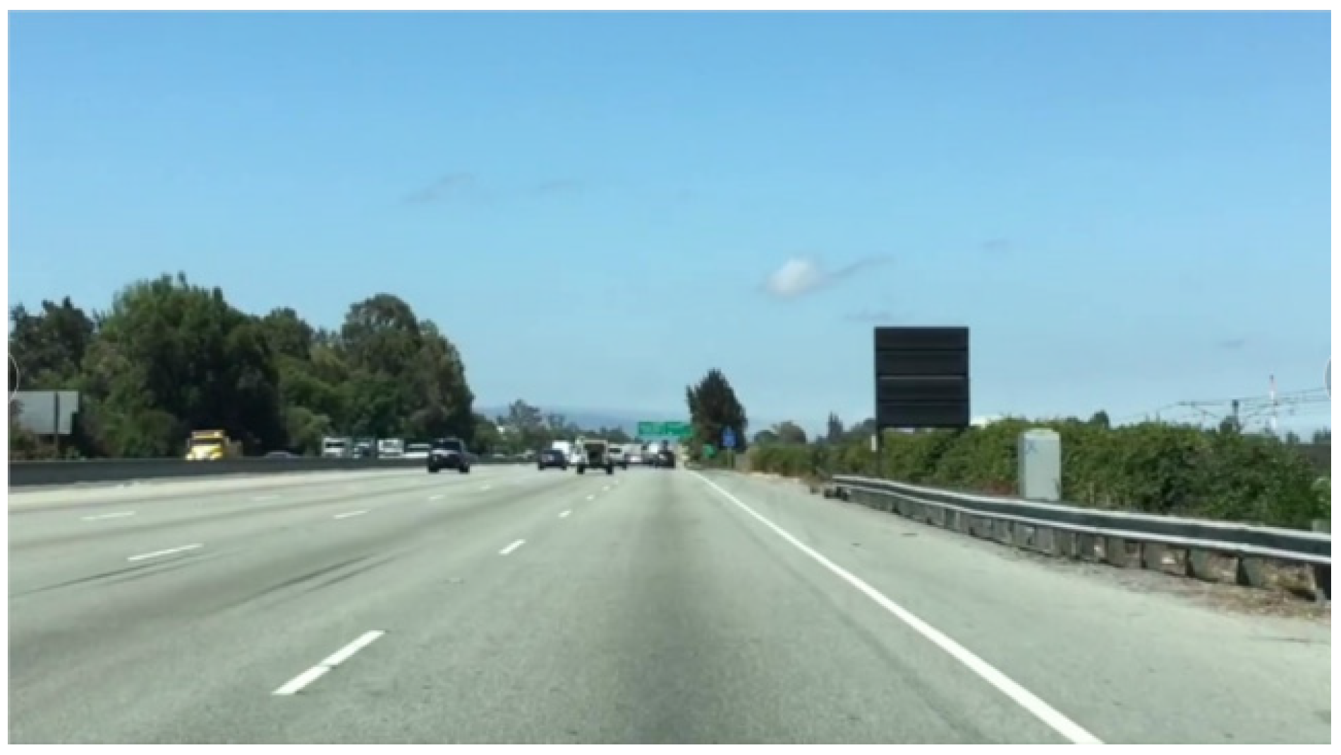
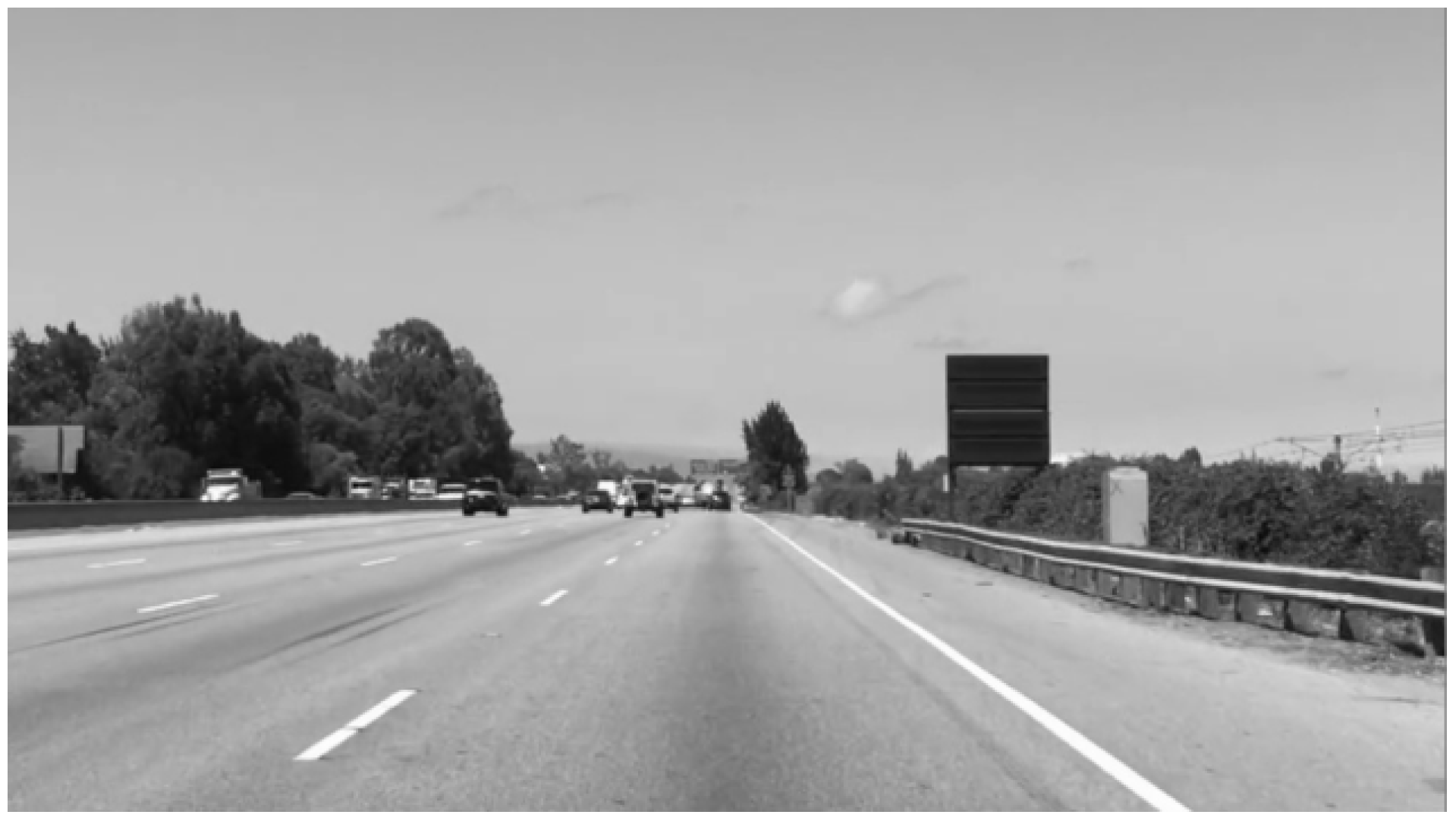
Figure 1 shows the original color image; the gray image shown in Figure 2 can be obtained by averaging the three color channels of each pixel. The conversion formula is presented in Equation (1), where represents the coordinates of the pixel point, , , and represent the R, G, and B three-channel values of the pixel point, respectively, and represents the gray value of the pixel point.

Figure 1.
Color image.

Figure 2.
Grayscale image.
2.2. Image Smoothing
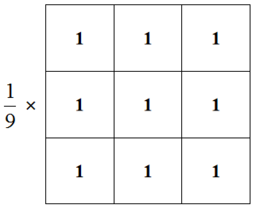
After obtaining a single-channel grayscale image, the proposed technique performs image processing in the spatial domain. Image smoothing is a method of spatial filtering. The smoothing filter plays a significant role in image denoising; thus, we used the mean filter to process the image. As shown in Figure 3, we set a 3 × 3 mask where the coefficients in the mask were all 1 and represented the average of the coefficients in the mask. At the same time, the edge of the image is usually processed by mirror expansion to prevent the loss of image edge information. Equation (2) represents the convolution process of an M × N image passing through an m × n weighted mean filter.
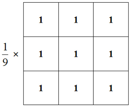
Figure 3.
A 3 × 3 mean filter template.
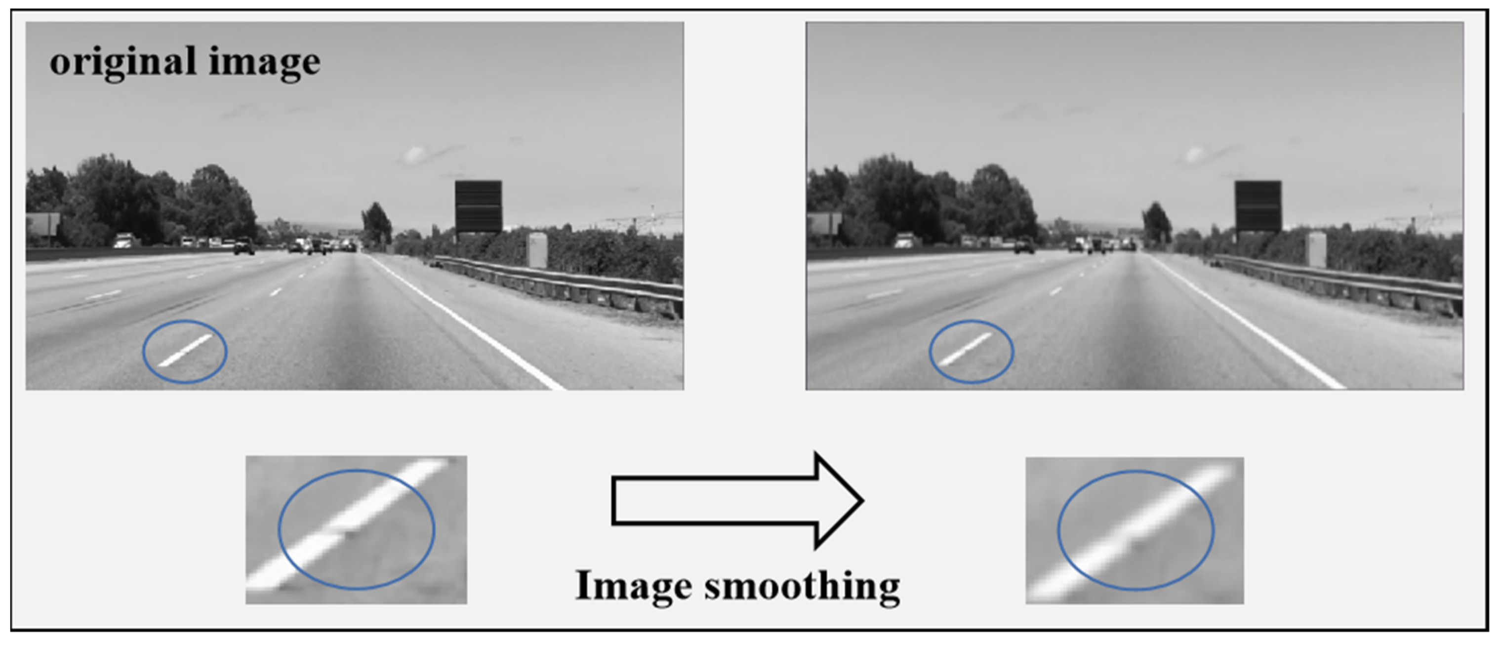
For masks of dimension m × n, m and n should be odd, represents the coefficient of the mask at , a and b represent the mask size, represents the gray value of the image pixel, the pixels in the neighborhood are averaged, and the final smoothed gray value is obtained. The image processed with the minimum mask of 3 × 3 is shown in Figure 4. It can be seen that after grayscale image smoothing, the image will be slightly blurred, which can effectively suppress the influence of noise pixels. From the details of the lane lines in Figure 4, it can be seen that the cracks in the original lane lines are used as noise pixels to interfere with the judgment of the entire lane line. After image smoothing, this noise can effectively be suppressed.

Figure 4.
Results of processing with a 3 × 3 mean filter.
2.3. Grayscale Transformation
In actual scenarios, the color of the lane line is quite different from the color of the background road surface. Therefore, if the lane lines and the road surface can be better distinguished, it will facilitate segmentation of the lane lines. As shown in Equation (3), the grayscale gamma transformation function can be constructed using the grayscale value of the lane line, higher than that of the road surface:
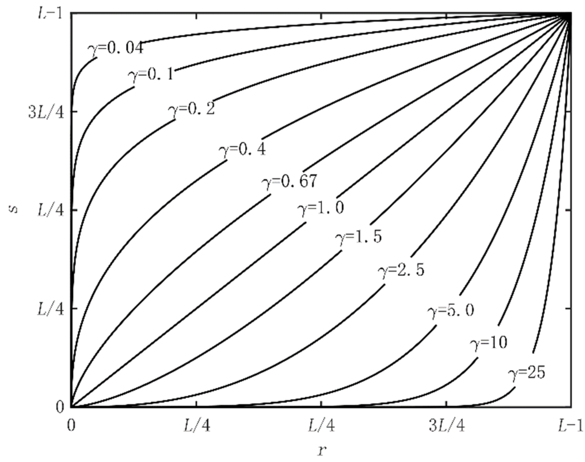
In Equation (3), is a normal number. In this study, we set , as the input gray level of the image, as the output gray level of the image, and as the gamma index which was used to adjust the contrast change in the image trend. The output image had higher contrast after applying gamma transform function to the original image. As shown in Figure 5, by changing the value of γ, a narrower gray-level value could be mapped to a wider range of gray-level output, and a wider gray level could also be mapped to a narrower range of gray-level output. In this way, lane line pixels with higher gray levels will be mapped to higher gray levels. For ground pixels with lower gray levels, the original gray level will be suppressed, which can better distinguish lane lines and road areas.

Figure 5.
Transformation curves corresponding to different γ values when c = 1.
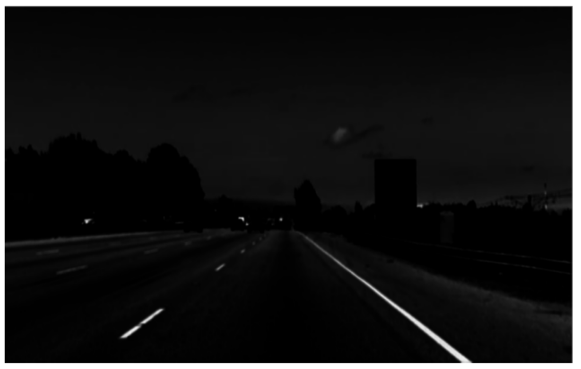
The results when γ is 5 and 10 correspond to Figure 6 and Figure 7, respectively. It can be seen that through the image grayscale transformation, the grayscale value of the lane line increased and that of the road surface was reduced, forming a more intuitive sense of contrast, also adding prior information for the segmentation of the lane lines below. However, the noise pixels in the road surface were also enhanced; thus, it is necessary to suppress the noise interference.
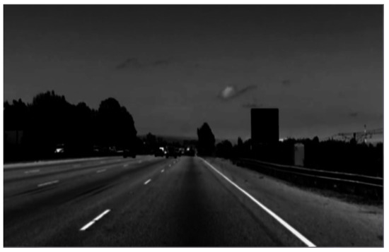
Figure 6.
The transformation result when γ is 5.
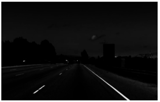
Figure 7.
The transformation result when γ is 10.
2.4. Road Region of Interest Extraction
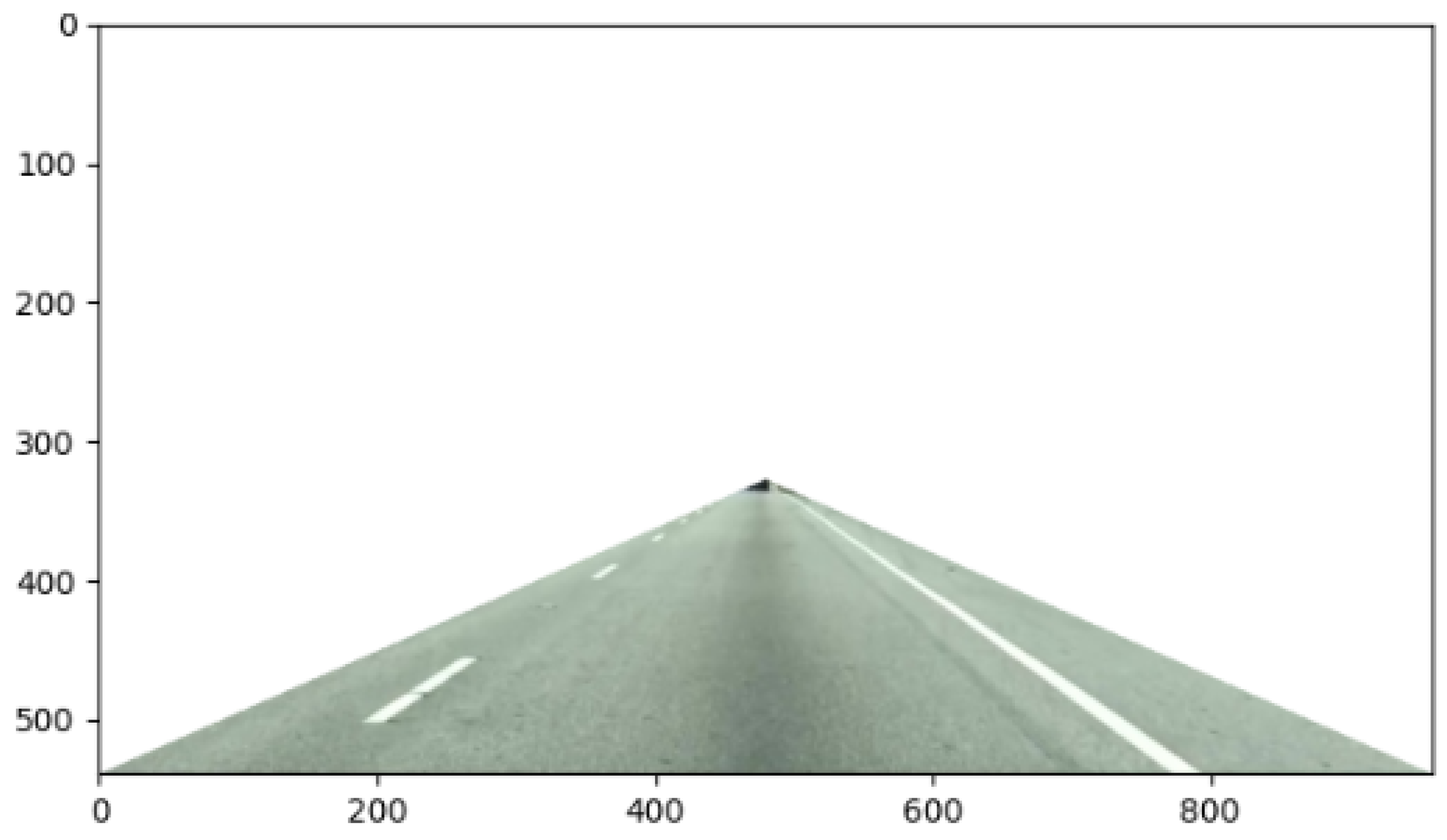
ROIs (regions of interest) can be used to acquire key information in an image. In lane line identification, the desired image is the lane line image in a certain region [18]. Masking other irrelevant information can reduce the model noise and improve the detection accuracy. The lane line generally appears in a specific region of the camera, as shown in Figure 8. This paper defines the front triangular field of view as the region of interest, which is located in the lower middle area of the image. For an image of size 1020 × 520, we specify that the left vertex of the triangle is (0,500), the right vertex is (1020,500), and the center point of the triangle is (510,330). Through image preprocessing and lane line search in this region, the operating efficiency will be greatly improved. Specifically, in this area, we first convert the image from color space to gray space, then use a 3 × 3 mask for smoothing, and finally use grayscale transformation with a γ of 10 to obtain the final preprocessed image.
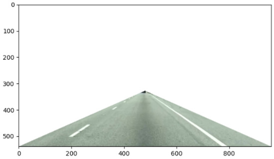
Figure 8.
Extraction of the ROI.
3. Markov Random Field
After image preprocessing, we modeled the image using Markov random field and further segmented out the lane line pixels. Markov random field (MRF) represents an undirected probabilistic graphical model which can classify different pixels in an image [19]. It has the relevant advantages of describing different labels of pixels. For an image, the position set of all pixel information is , the random variable set associated with each pixel position is , and the neighborhood set of each position pixel is , where N represents the neighborhood range; in this study, we set N = 4. As in Equation (4), if a Markov random field is to be established, the model must meet the Markov features:
Among them, Wn represents the category of the n pixel, and in the lane line detection task we specify that the categories are only lane lines and non-lane lines. WS represents the prior category of the image as a whole, and WEn represents the category of the pixel n neighborhood range. P (Wn|Ws) represents the conditional probability that the class of pixel n is Wn when the global class is WS. This feature explains the principle of conditional independence in undirected graph models, i.e., given a neighborhood, each pixel variable should be conditionally independent of each other.
We further modeled the image by MRF and specified that the image pixels corresponded to the nodes of the MRF one-to-one. In the MRF model, each node represents a variable, and the edge between the nodes depicts the dependencies between variable levels, as shown in Equation (5). The joint probability of the variables is described as the product of potential functions:
where Z is the normalization factor of the joint probability distribution to ensure that the result is an effective probability distribution, usually called the partition function, and the factor represents the jth potential function, which maps the set of random variables to the real number domain and returns a non-negative value. This value depends on the subset state of the variable set .
In the field of computer vision and image processing, we should not only consider the continuity of adjacent pixels, but also ensure the correct classification of discrete pixels. Therefore, it is necessary to use paired Markov random fields to obtain joint probability distributions by adding node potential functions, as shown in Equation (6).
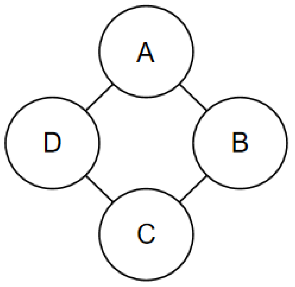
where is the energy potential function at the node p, and is the energy potential function on the edge connected to the adjacent nodes p and q. Figure 9 shows a 2 × 2 MRF graphic model. By defining the energy potential function in the neighborhood of four nodes and that of a single node, the joint probability distribution of the model can be determined, as shown in Equation (7):
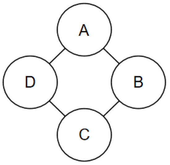
Figure 9.
Example MRF graphic model.
4. MRF Reasoning Based on Graph Cut Method
Probabilistic reasoning is equivalent to model solving. When the joint probability distribution is known, the goal is to determine the maximum posterior probability state of the model through reasoning, and the combination with the highest probability is viewed as the optimal classification [20]. Therefore, this study used the graph cut method for accurate reasoning of the MRF, which can support effective classification according to pixel information.
4.1. Maximum Posterior Probability Reasoning
After using Markov random fields for image modeling, the image processing problem is transformed into a problem of maximum posterior probability reasoning defined in the MRF, as shown in Equation (8):
where the maximum posteriori probability p (x) is proportional to the continuous product of the paired MRF energy potential function. The maximum posteriori probability is equivalent to the problem of obtaining a minimized the energy E (x); thus, it is transformed into the logarithmic domain for a solution. Therefore, it can be indicated through Equation (9):
where represents the observation cost under a given state at the single pixel p, which can also be regarded as the cost of sample classification. Similarly, represents the cost function of placing category labels at the two adjacent pixels p, q. The normalization factor Z in the MRF is equivalent to a constant in reasoning; therefore, it can be omitted.
4.2. Binary Graph Cut Method
The graph cut method is widely used in computer vision and image processing, mainly to solve the problem of energy minimization [21]. When using the binary graph cut method for accurate reasoning, the value of each random variable should be two, and the potential function between adjacent variables should meet the inequality relationship of Equation (10):
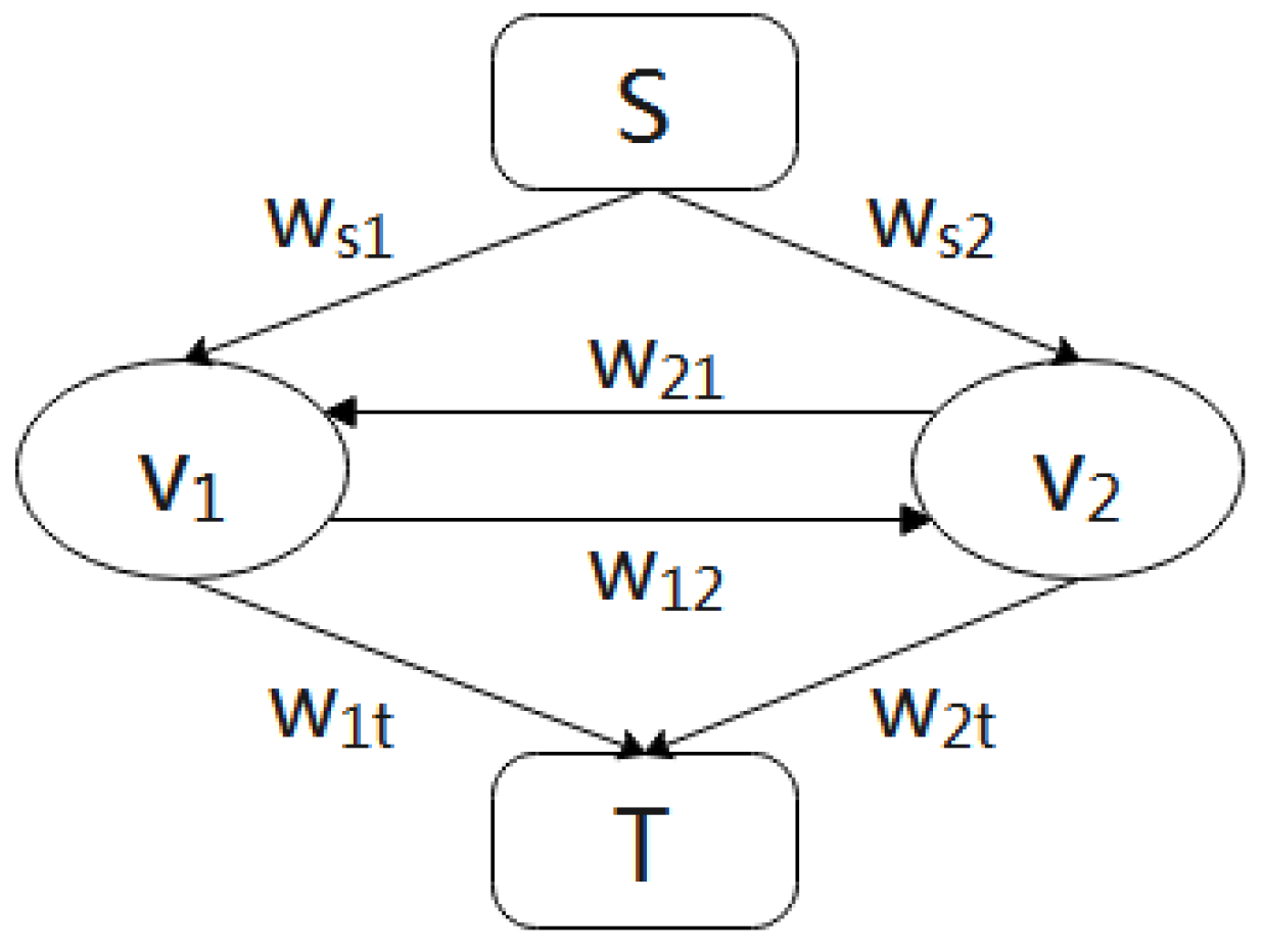
where represents the corresponding energy potential function value when the pixels p and q take different gray values. This inequality ensures that there will be no negative cost. For the MRF model, it can be represented by a directed graph: . Here, V represents the set of variables and E represents the set of adjacent variable edges. The edge weights of graph G are assigned according to the energy function. Each node potential function and edge potential function of the energy function are assigned to graph G in turn through certain rules; then, the edge weights after assignment are accumulated, and finally, a weighted graph G is formed.
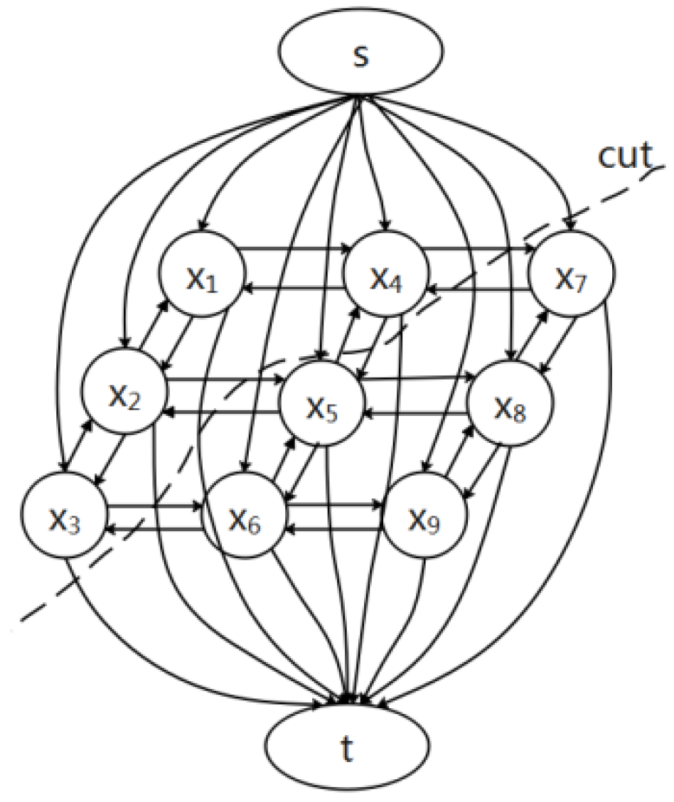
Through the s–t cutting graph G, the corresponding maximum posteriori probability is obtained. As shown in Figure 10, each node in the figure corresponds to a pixel. The node set V is divided into two disconnected subsets, S and T. Here, the source node s is in the set S, and the sink node t is in the set T. When a node u belongs to S, the node variable takes the value of 0; when the node u belongs to T, the node variable takes the value of 1. Adjacent nodes in the grid are connected by a pair of directed edges, the source node is connected to each node by a directed edge, and the sink node is also connected to each node by a directed edge.
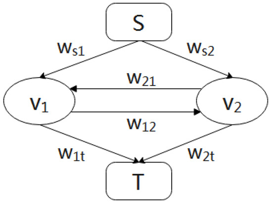
Figure 10.
Directed graph G.
As shown in Figure 11, the minimum s–t segmentation problem is to find a segmentation to minimize the weights of all edges. It can be understood that when classifying pixels, the cost allocated to S and T is . Considering the attributes of a single pixel and the continuity of the pixels in the neighborhood, the minimum cost can be calculated, which is specifically expressed as in Equation (11).
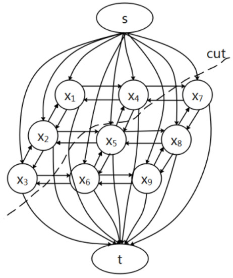
Figure 11.
s–t segmentation.
In conclusion, the energy minimization problem can be solved by s–t segmentation of the directed graph G, and each variable can be accurately classified by selecting an appropriate energy potential function.
4.3. Maximum Flow Problem
According to [22], the minimum segmentation method is equivalent to the maximum flow from the source node to the sink node. For the maximum flow problem, there are many algorithms with time complexity as the polynomial level [23]. In a given graph G, connected by directed edges, each edge has a non-negative capacity , and there are two vertices, s and t, called the source and sink nodes, respectively.
In the analysis of the maximum flow problem, when considering the capacity of each edge, the goal is to push as much “flow” from the source node to the sink node as possible.
The augmented path algorithm is often used to solve the maximum flow problem, which is an iterative process of the “flow”. First, a path from the source node s to the sink node t is found, and the capacity of the path should be greater than zero. Then, the maximum “flow” flowing through this path is calculated. For an edge constrained by a path of minimal volume, all paths along the edge will lose the portion of “flow” so that a new saturated edge is formed. This process is iterated until there are no paths that satisfy the condition.
The saturated edge in the maximum flow problem can isolate the source and sink nodes; therefore, the saturated edge can be used to achieve the purpose of segmentation. The minimum cost is achievable by reasonably choosing the energy function. Therefore, the maximum flow problem is equivalent to the minimum s–t segmentation problem.
4.4. Determination of Energy Potential Function
In Markov random field, the energy potential function is used to reflect the interaction between nodes, and is equivalent to the cost function of the minimum s–t segmentation. Each pixel in the image is independent of each other, and the energy potential function can be considered to obey the Gaussian distribution, which can be expressed by Equation (12):
where z is the normalization factor; parameter T is a non-zero constant which is used to indicate the concentration degree of the classification; C is the set of all the potential groups; and is the potential energy value of the potential groups which indicates the coupling degree between different potential groups. It can be expressed as shown in Equation (13):
where β is an adjustable parameter that is used to specify the degree of the difference between the s and t set potential functions. Through the above formulas, the energy minimization problem can be solved iteratively, i.e., the lane line segmentation pixels are obtained.
In this study, first, the task of lane recognition was transformed into the problem of energy segmentation between reasoning pixels by establishing a Markov model on the preprocessed image. Then, the energy potential function was determined and applied to s–t segmentation; finally, the optimal segmentation strategy was obtained by introducing the maximum flow problem for completing the recognition of lane line pixels.
5. Experimental Results and Analysis
5.1. Experimental Environment and Simulation
For the above MRF modeling and reasoning, related experiments were conducted. The experimental environment was Linux Ubuntu 20.4, CUDA 11.0, and the code writing was completed using Python 3.7 on a 4 GB RAM computer.
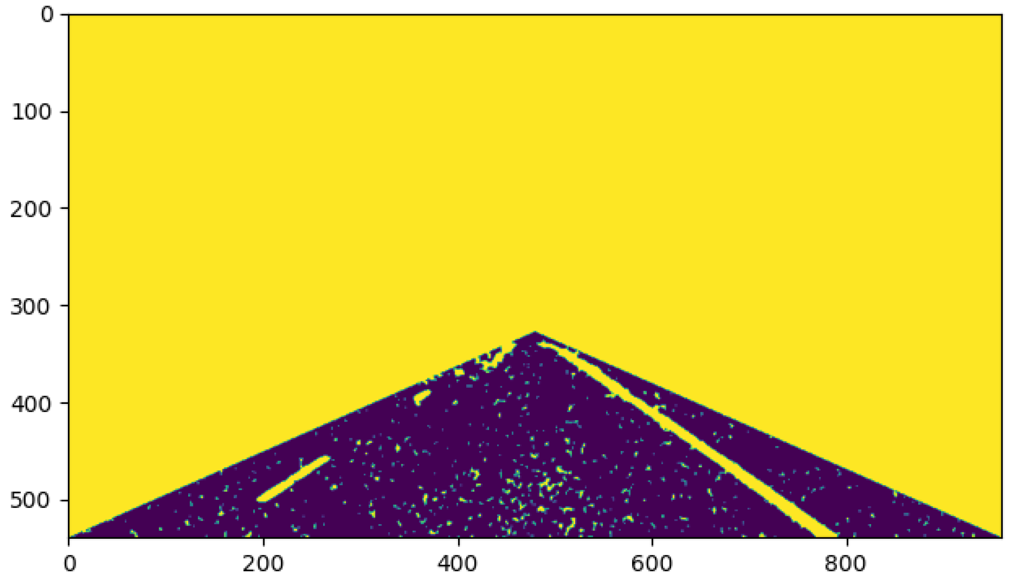
First, the image was preprocessed. Figure 12 shows the result after the original image was smoothed by the mean filter and processed by the grayscale transformation of gamma = 4, with the region of interest of the lane line intercepted; it can be seen that the road surface and the lane line were not segmented. Figure 13 shows the results after three iterations by solving the maximum a posteriori probability of MRF and combining the minimum s–t segmentation algorithm; it can be seen that the lane line and the road surface in the image were basically segmented, although due to the interference from abundant noise points, the noise points were wrongly recognized as a class with lane lines.
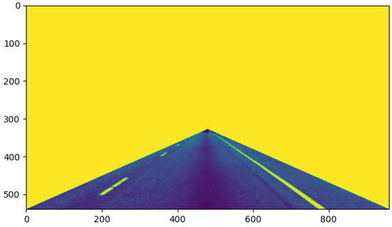
Figure 12.
Preprocessed image.

Figure 13.
Result after three iterations.
Figure 14 shows the result after six iterations. Compared with Figure 13, the segmentation accuracy was significantly higher, but there were still some noise points that affected the accurate segmentation of the lane lines. Therefore, the number of iterations still needed to be increased. Figure 15 shows the result after ten iterations. It can be seen that the lane line and the road surface were clearly separated, which indicates the high-quality semantic information between the lane line and the road surface. At this time, the lane line and the road mask had different labels, which can help to quickly complete the lane line recognition.

Figure 14.
Result after six iterations.
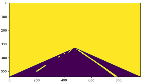
Figure 15.
Result after ten iterations.
5.2. Model Quantitative and Qualitative Analysis
To quantitatively analyze the performance of our model, we implemented lane line detection on the more challenging Tusimple dataset [13]. The Tusimple dataset contains 2000 real-world autonomous driving images captured by in-vehicle cameras with accurate annotations and evaluation criteria. The Tusimple dataset [13] uses accuracy to evaluate the detection. The expression of accuracy is given in Equation (14), where Npred denotes the lane line prediction result and Ngt denotes the lane line ground truth label.
We selected studies [8,11] with which we could compare our method on single-frame running time and accuracy. As shown in Table 1, we separately conducted ablation experiments for image preprocessing. When no image preprocessing was used, our method was slightly slower than those reported in reference [11], which was because lane line fitting by the Canny-operator-based method [11] is a global one-shot process. However, our MRF was a joint model of local and global images and had higher computational complexity than those presented in reference [11]. However, the best performance was obtained in detecting accuracy. After using the image preprocessing technique proposed in this paper, our method significantly outperformed the data-driven method in reference [8] (+3.02%). Moreover, our method only increased the running time by 11 ms and achieved an accuracy of 87.61%, an increase of 2.97%.

Table 1.
Algorithm comparison and ablation experiments.
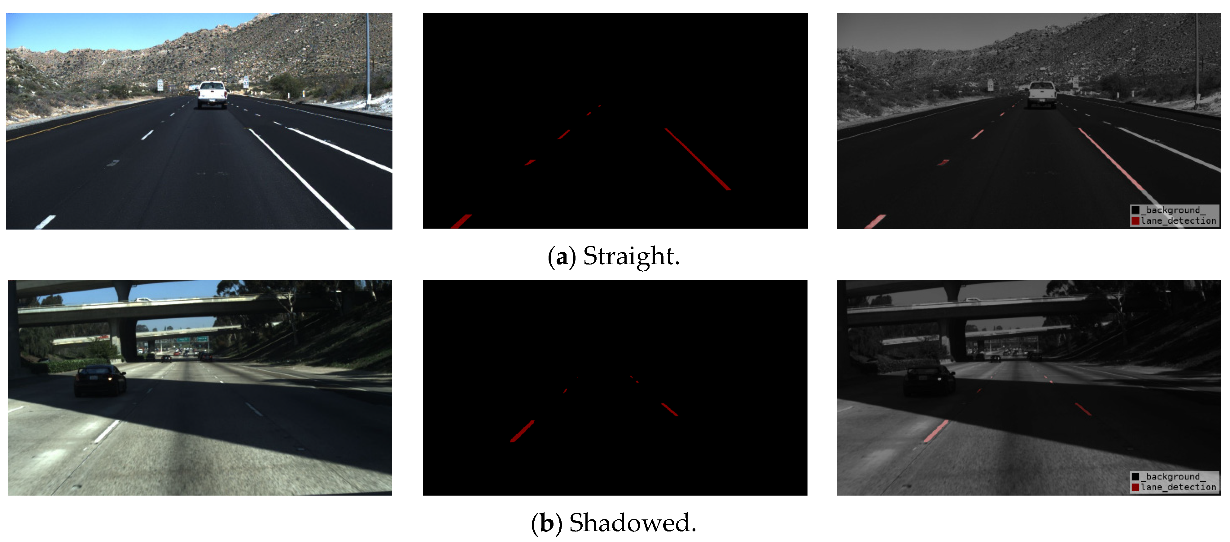
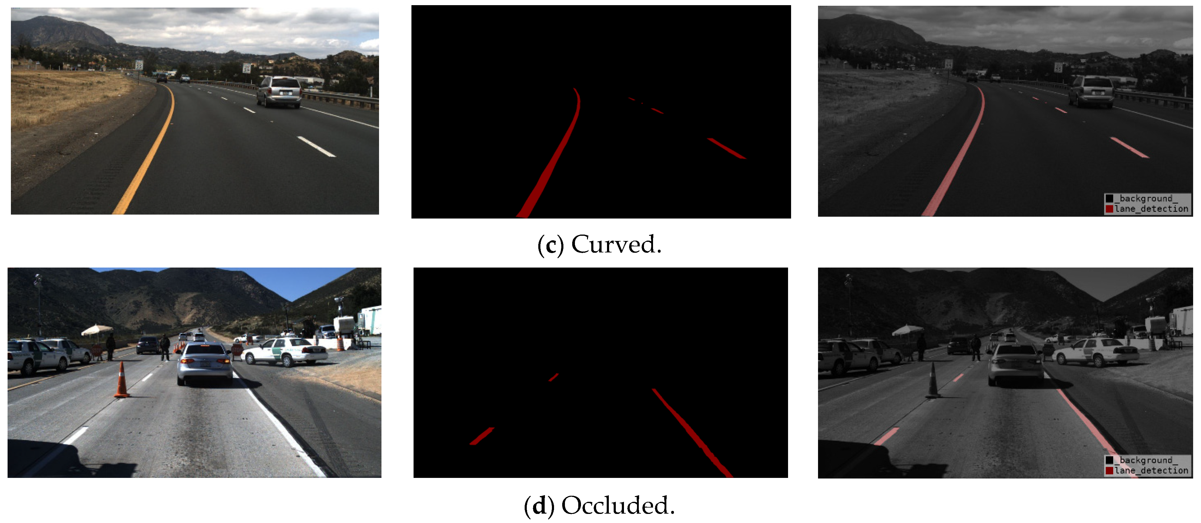
To more intuitively demonstrate the positive effect of our method, we selected different scenarios from the Tusimple dataset for lane line detection. As shown in Figure 16, the left is the original image, the middle is the result of lane line detection using our method, and the right is the image after masking the detection result with the real image. As shown in Figure 16a, our method demonstrated superior performance under well-lit and straight lane lines. As shown in Figure 16b, our method could still accurately detect lane lines under shadows. As shown in Figure 16c, our method had a strong fitting ability for curved lane lines. As shown in Figure 16d, occluded lane lines were one of the main challenges for our detection, and our method still has some shortcomings when detecting lane lines with fewer pixels at long distances.


Figure 16.
Lane line detection results on the Tusimple dataset.
6. Conclusions
Lane line recognition based on vision can extract track coordinates from images captured by optical sensors and provide key lane information for the decision-making processes and control of autonomous driving systems, which is the premise of vehicles travelling autonomously.
This paper proposes a lane line identification method based on Markov random field. First, the original image collected by the camera was preprocessed; then, the processed image was modeled based on Markov random field theory, and energy potential function was constructed based on the lane line segmentation task. Finally, the model was solved using the graph cut method. Experiments showed that, after ten iterations, the algorithm could quickly and accurately extract the pixels of the lane line, thus completing the semantic segmentation between the lane line and the road surface.
Author Contributions
Conceptualization, F.D. and Q.Z.; data curation, F.D.; funding acquisition, A.W. and Q.Z.; methodology, F.D. and A.W.; project administration, A.W.; supervision, A.W.; visualization, F.D.; writing—original draft preparation, F.D.; writing—review and editing, F.D. and Q.Z. All authors will be informed about each step of manuscript processing including submission, revision, revision reminder, etc., via emails from our system or assigned Assistant Editor. All authors have read and agreed to the published version of the manuscript.
Funding
The authors would like to thank the financial support from the academic support project for top-notch talents in disciplines (majors) in colleges and universities, No. GXBJZD20106, and the key natural science research projects of colleges and universities in Anhui Province, No. KJ2020A1116 and No. KJ2019A1154.
Institutional Review Board Statement
Not applicable.
Informed Consent Statement
Not applicable.
Data Availability Statement
Not applicable.
Conflicts of Interest
The authors declare no conflict of interest.
References
- Li, M.; Lyu, H.; Wang, F.; Jia, D. An Intelligent Vehicle Robust Lane Line Identification Method Based on Machine Vision. China Mech. Eng. 2021, 32, 242–251. (In Chinese) [Google Scholar]
- Kavya, R.; Md Zakir Hussain, K.; Nayana, N.; Savanur Sanjana, S.; Arpitha, M.; Srikantaswamy, R. Lane Detection and Traffic Sign Recognition from Continuous Driving Scenes Using Deep Neural Networks. In Proceedings of the 2nd International Conference on Smart Electronics and Communication, ICOSEC, Tamil Nadu, India, 7–9 October 2021; pp. 1461–1467. [Google Scholar]
- Huang, S.-T.; Chan, Y.-C.; Lin, Y.-C.; Lin, C.-L. Time to Lane Crossing Estimation Using Deep Learning-Based Instance Segmentation Scheme. In Proceedings of the ICAAI 2019 the 3rd International Conference on Advances in Artificial Intelligence, Istanbul, Turkey, 26–28 October 2019; pp. 29–34. [Google Scholar]
- Lin, Q.; Youngjoon, H.; Hahn, H. Real-Time Lane Detection Based on Extended Edge-Linking Algorithm. In Proceedings of the 2nd –International Conference on Computer Research and Development, ICCRD, Washington, DC, USA, 7–10 May 2010; pp. 725–730. [Google Scholar]
- Ng, H.-F.; Kheng, C.-W.; Lin, J.-M. A weighting scheme for improving Otsu method for threshold selection. J. Comput. 2016, 27, 12–21. [Google Scholar]
- Wu, P.-C.; Chang, C.-Y.; Lin, C.H. Lane-mark extraction for automobiles under complex conditions. Pattern Recognit. 2014, 47, 2756–2767. [Google Scholar] [CrossRef]
- Wang, Y.; Shen, D.; Teoh, E.K. Lane detection using spline model. Pattern Recognit. Lett. 2000, 21, 677–689. [Google Scholar] [CrossRef]
- Mechat, N.; Saadia, N.; M’Srdi, N.K.; Djelal, N. Lane Detection and Tracking by Monocular Vision System in Road Vehicle. In Proceedings of the 2012 5th International Congress on Image and Signal Processing, CISP, Chongqing, China, 16 October 2012; pp. 1276–1282. [Google Scholar]
- Kang, D.-J.; Jung, M.-H. Road lane segmentation using dynamic programming for active safety vehicles. Pattern Recognit. Lett. 2003, 24, 3177–3185. [Google Scholar] [CrossRef]
- Teo, T.Y.; Sutopo, R.; Lim, J.M.-Y.; Wong, K.S. Innovative lane detection method to increase the accuracy of lane departure warning system. Multimed. Tools Appl. 2021, 80, 2063–2080. [Google Scholar] [CrossRef]
- Yu, B.; Jain, A.K. Lane Boundary Detection Using a Multiresolution Hough Transform. In Proceedings of the IEEE International Conference on Image Processing, Santa Barbara, CA, USA, 26–29 October 1997; Volume 2, pp. 748–751. [Google Scholar]
- Chen, W.; Wang, W.; Wang, K.; Li, Z.; Li, H.; Liu, S. Lane departure warning systems and lane line detection methods based on image processing and semantic segmentation: A review. J. Traffic. Transp. Eng. 2020, 7, 748–774. [Google Scholar] [CrossRef]
- Neven, D.; De Brabandere, B.; Georgoulis, S.; Proesmans, M.; Van Gool, L. Towards End-to-End Lane Detection: An Instance Segmentation Approach. In Proceedings of the 2018 IEEE Intelligent Vehicles Symposium IV, Suzhou, China, 26–30 June 2018; pp. 286–291. [Google Scholar]
- Savant, K.V.; Meghana, G.; Potnuru, G.; Bhavana, V. Lane Detection for Autonomous Cars Using Neural Networks. In Proceedings of the Machine Learning and Autonomous Systems—Proceedings of ICMLAS 2021, Smart Innovation, Systems and Technologies, Tamil Nadu, India, 24–24 September 2022; Volume 269, pp. 193–207. [Google Scholar]
- Gao, Q.; Feng, Y.; Wang, L. A Real-Time Lane Detection and Tracking Algorithm. In Proceedings of the 2017 IEEE 2nd Information Technology, Networking, Electronic and Automation Control Conference, ITNEC, Chengdu, China, 15–17 December 2017; Volume 2018, pp. 1230–1234. [Google Scholar]
- Zhang, X.; Yang, W.; Tang, X.; Liu, J. A fast learning method for accurate and robust lane detection using two-stage feature extraction with YOLO v3. Sensors 2018, 18, 4308. [Google Scholar] [CrossRef] [Green Version]
- Petwal, A.; Hota, M.K. Computer Vision Based Real Time Lane Departure Warning System. In Proceedings of the 2018 IEEE International Conference on Communication and Signal Processing, ICCSP, Chennai, India, 3–5 April 2018; pp. 580–584. [Google Scholar]
- Cao, J.; Song, C.; Song, S.; Xiao, F.; Peng, S. Lane detection algorithm for intelligent vehicles in complex road conditions and dynamic environments. Sensors 2019, 19, 3166. [Google Scholar] [CrossRef] [PubMed] [Green Version]
- Nsimba, C.B.; Levada, A. An information-theoretic wavelet-based texture descriptor using Gaussian Markov random field models. Multimed. Tools Appl. 2019, 78, 31959–31986. [Google Scholar] [CrossRef]
- Zhao, J.; Huang, G.; Zhao, Z. SAR image change detection based on fuzzy Markov random field model. Int. Arch. Photogramm. Remote Sens. Spat. Inf. Sci.—ISPRS Arch. 2018, 42, 2371–2374. [Google Scholar] [CrossRef] [Green Version]
- Liu, C.; Bao, J.; Yang, J.; Ma, W.; Wang, J. Coastline detection in polarimetric SAR images using Markov random field segmentation based on mixture Wishart distribution. Syst. Eng. Electron. 2020, 42, 568–574. (In Chinese) [Google Scholar]
- Lin, Y.-K.; Chen, S.-G. A maximal flow method to search for d-MPs in ochastic-flow networks. J. Comput. Sci. 2017, 22, 119–125. [Google Scholar] [CrossRef]
- Wang, C.; Zhang, Y.; Wang, X. SAR Image Change Detection Based on Variational Method and Markov Random Field Fuzzy Local Information C-Means Clustering Method, Wuhan. Geomat. Inf. Sci. Wuhan Univ. 2021, 46, 844–851. (In Chinese) [Google Scholar]
Publisher’s Note: MDPI stays neutral with regard to jurisdictional claims in published maps and institutional affiliations. |
© 2022 by the authors. Licensee MDPI, Basel, Switzerland. This article is an open access article distributed under the terms and conditions of the Creative Commons Attribution (CC BY) license (https://creativecommons.org/licenses/by/4.0/).

