Collaborative Optimization of the Battery Capacity and Sailing Speed Considering Multiple Operation Factors for a Battery-Powered Ship

Abstract

In the context of harsh emission control and ecological environment protection, the shipping industry is transforming and upgrading towards greening, decarburization, and electrification. Battery-powered all-electric inland ships have been attracting increasingly attention. However, its initial investment cost is much more expensive than a traditional diesel-driven mechanical ship because lithium-ion batteries are currently expensive. Hence, a suitable battery size and efficient energy management strategy for ship sailing are very important for a battery-powered ship. In this paper, a novel joint optimization method of the sailing speed and battery capacity, which considers the interaction between battery size and sailing speed as well as multiple operation factors, such as freight demand and battery life, and port electricity price, is proposed to fully exploit the battery-powered ships’ application potential. Moreover, a joint optimization model of the sailing speed and battery energy consumption model considers the battery-powered ship’s characteristics and waterway characteristics. Next, a solution algorithm for the proposed joint optimization model is established to achieve joint decision-making regarding the sailing speed and battery size. Finally, case studies are conducted to demonstrate the flexibility and effectiveness of the proposed method. The results show that the proposed method can obtain the optimal sailing speed and the corresponding battery capacity synchronously when the actual transportation scenario is fixed. Moreover, the battery initial investment cost can be effectively reduced with the prosed method.

1. Introduction

As the amount of greenhouse gas that is generated by ships increases, the international maritime organization (IMO) has launched an ambitious target whereby all the ships built after 2025 should achieve 30% greenhouse gases (GHGs) emission reductions compared with 2005 [1,2]. Hence, new ways must be found to reduce emissions of greenhouse gas. Compared to ocean transport, inland waterway transport has not been paid enough attention to for a long time [3], and more than 95% of inland ships are conventional diesel-driven mechanical ships with low energy efficiency and serious environmental pollutants. As a result, a large amount of inland water transport can cause serious environmental pollution in areas along the river [4]. Though many solutions have been proposed to mitigate ship GHGs emissions, two popularly accepted ways are ship electrification and renewable energy use [5]. The battery-powered ship completely satisfies the above two requirements as the charged power can be generated from renewable energy resources (RESs), such as wind and solar radiation, and the ship power system is constructed by integrated power system (IPS) technology. In addition, the battery-powered ship can be considered as an energy storage device when it berths at the dock, and it can take part in the energy shifting operation of the land power network [6].

In an all-electric ship (AES), the propulsion and service loads are both met by the onboard power sources with the use of IPS technology and complex energy management [7,8]. Thus, in some cases, they are viewed as a “mobile microgrid”. IPS can easily integrate optimal power management technology, energy storage systems (ESS), and different kinds of renewable energy resources. It can reduce the redundancy of the onboard components of main engines in most cases and increase the system energy efficiency [9]. Concurrently, the electric propulsion system of AES can provide more flexible and controllable navigation than the fixed mechanical drives of traditional ships. Therefore, AES is considered an irreversible trend for future ship designs.

As the RES utilization technologies, such as solar energy and offshore wind power, are widely used on land, the promotion and application of marine RESs have become an inevitable trend, especially on ships [10,11]. Ruoli Tang et al. developed an optimal energy management model and control methodology to ensure the operational safety and efficiency of a ship with photovoltaic/battery/diesel/cold-ironing. The results indicated that the proposed method can reduce the ship’s electricity cost and increase the solar use [12]. Sun Fang et al. proposed a data-driven generation and demand-side robust coordination strategy considering the PV generation uncertainties. The simulation results show that the extreme learning machine-based method can well characterize the PV uncertainties [13]. Hai Lan et al. proposed a method for determining the optimal size of the photovoltaic (PV) generation system, the diesel generator, and the energy storage system in a ship power system that minimizes the investment cost, fuel cost, and CO₂ emissions [14]. Yuanchao Qiu et al. conducted a techno-economic analysis and an environmental performance assessment of the integration of the photovoltaic system [15]. The above researches indicate that energy storage is an indispensable part of the ship with renewable energy resources. The more energy storage is integrated, the more stable the ship’s power system.

For better control and operation AES, protection issues [16], designing advanced control strategies [17], reactive power planning [18], and distributed energy resource management [19] are all investigated and discussed. To reduce the ship’s pollution and energy consumption effectively, Zheming Jin et al. proposed a hierarchical control method for a DC distribution-based AES to solve the power management and power quality issues. The inverse-droop control framework is implemented to the hybrid ESSs [20]. Samy Fadel et al. proposed an accommodated control strategy for a medium-voltage direct current (MVDC) based AES with energy storage systems and diesel generators. The results show that it can effectively reduce the ship’s emissions and improve the energy efficiency [21]. Jun Hou et al. developed an MPC-based hybrid energy storage system (HESS) control strategy of an AES to alleviate the power fluctuations introduced by the propulsion loads. Their case study shows that the cooperative operation of the battery and flywheel can mitigate the load fluctuations effectively [22]. However, compared to the above approaches, sailing speed optimization is the most effective [23]. Zhi Yuan et al. established a joint optimization model for the sailing route and speed of an inland ship based on an energy consumption model that considers multiple environmental factors [24]. Xiong Yifan et al. discussed an inland ship speed optimization problem considering the loading and unloading uncertainty. An interval number programming method was constructed to solve the nonlinear optimization problem [25]. Kai Wang et al. proposed a joint optimization model of the sailing route and speed for a sea ship, which is based on an energy consumption model [26].

A battery-powered ship is a type of special AES that has no pollutant air emissions and can friendly integrate renewable energy resources on board or use the energy generated by RESs. According to the investigation of Research and Markets, the market scale of battery-only power ships will become 12.32 billion dollars, and hundreds of ships will use batteries as their only power source shortly. However, similar to the electric vehicle, the battery purchasing cost is too expensive [27,28], as a large amount of deployment of batteries has caused a large investment cost for the customers. To the best of the authors’ knowledge, there is no literature discussing the battery size and operation optimization of the battery-only-powered ships. Some studies have investigated ESS size optimization problems of hybrid energy ships. Kyunghwa Kimerature et al. proposed a battery sizing method 500 TEU container ship, in which the battery is used as the main power source in port in/out mode and harbor mode and used as the assistant power source in other modes [4]. Xianqiang Bao et al. proposed a joint optimization method of ESSs size and power energy management storage to minimize the ship operation cost over its life. The battery size was used to reduce the fuel consumption of an engineering ship [29]. M. Othman et al. proposed a modeling method for battery size optimization, dividing the whole optimization problem into two sub-problems to reduce the computational burden of sim optimization [30].

In this paper, a joint optimization of battery capacity deployment and ship sailing speed is proposed to maximally reduce the investment cost and operation cost and maximize the revenue of the battery-only powered ships to help more ship owners determine whether it is worth building a battery ship.

The remainder of this study is structured as follows. The description of the employed methodology is provided in Section 2. In Section 3, the details of the case ship study are presented, including the required input for the implementation, the considered design scenarios based on different marine propulsion systems, and the analysis of the vessel’s energy consumption. The equivalent battery-powered version is analyzed to determine the battery size, capacity, and electric power demand.

2. Problem Description

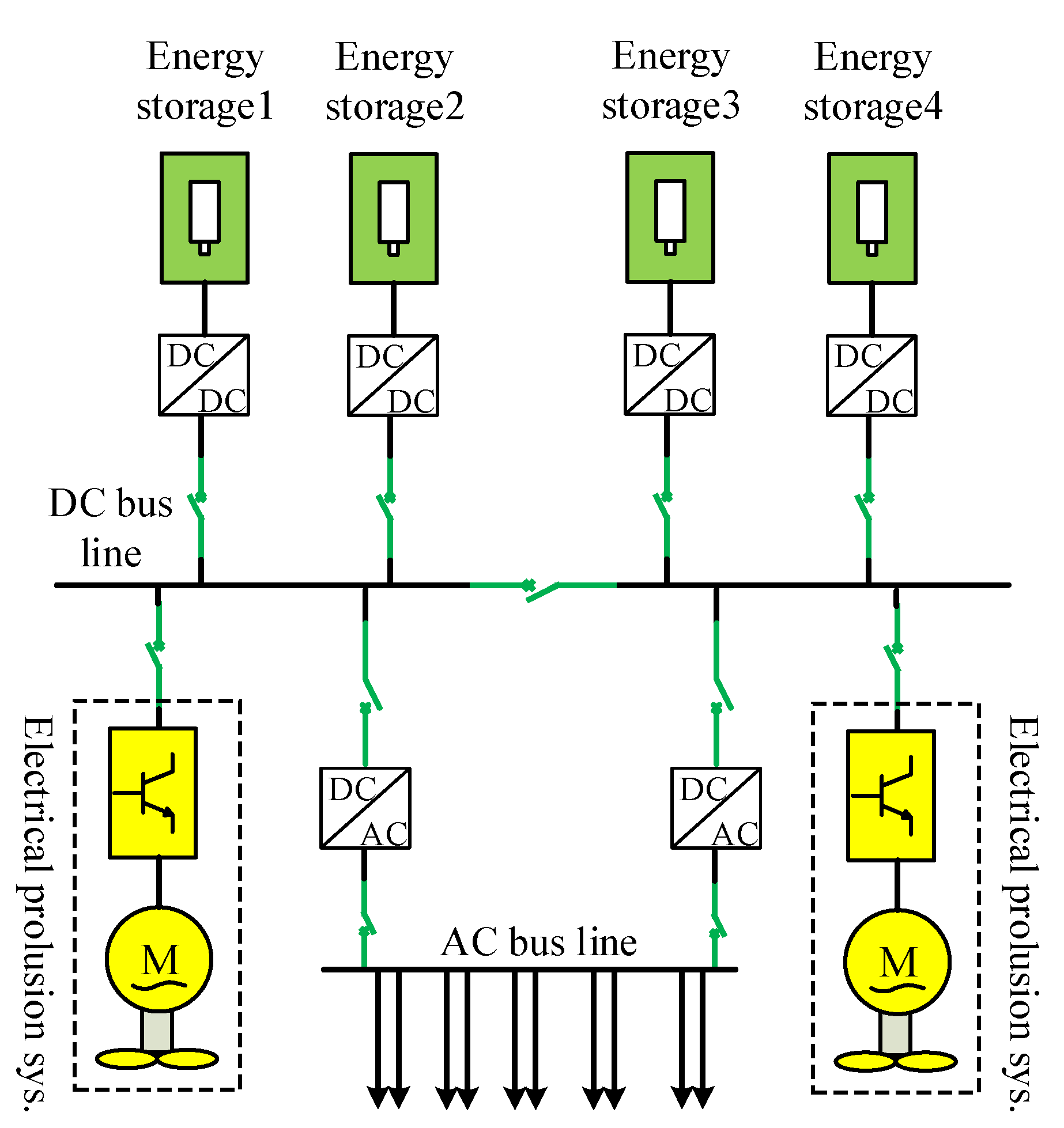
2.1. Battery-Only Powered Ship IPS Description

A generic diagram of battery-only powered IPS is shown in Figure 1. It can be considered as an independent shipboard DC microgrid [31]. Compared to the battery-only powered AC ship microgrid, the energy management of DC microgrid is simpler and the power supplying quality is higher. Hence, most battery-only powered IPS are constructed as a DC microgrid architecture. The number of battery units and battery topology are usually determined by the battery capacity and output voltage. For the inland ships, due to the propulsion load demand being usually lower than 1 MW, the bus voltage is usually lower than 1000 V. The battery power output and on/off status are determined by the energy management system (EMS). The most significant difference between the battery-only powered ships and the conventional mechanical ships is that the total ship available energy is limited to the former and can be considered as infinite regarding the latter. Therefore, the sailing speed and battery capacity optimization are more important to battery-only powered ships than conventional mechanical ships. Correspondingly, due to the power charging station limit, battery-only power ships are usually the only suitable fixed-route transportation, which means the route optimization does not affect them.

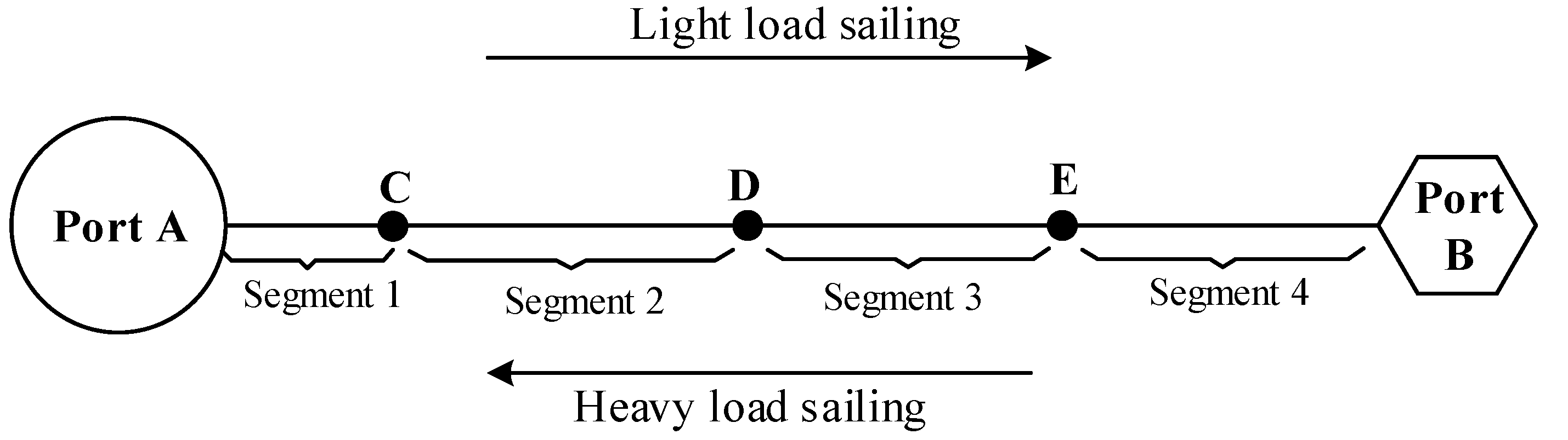
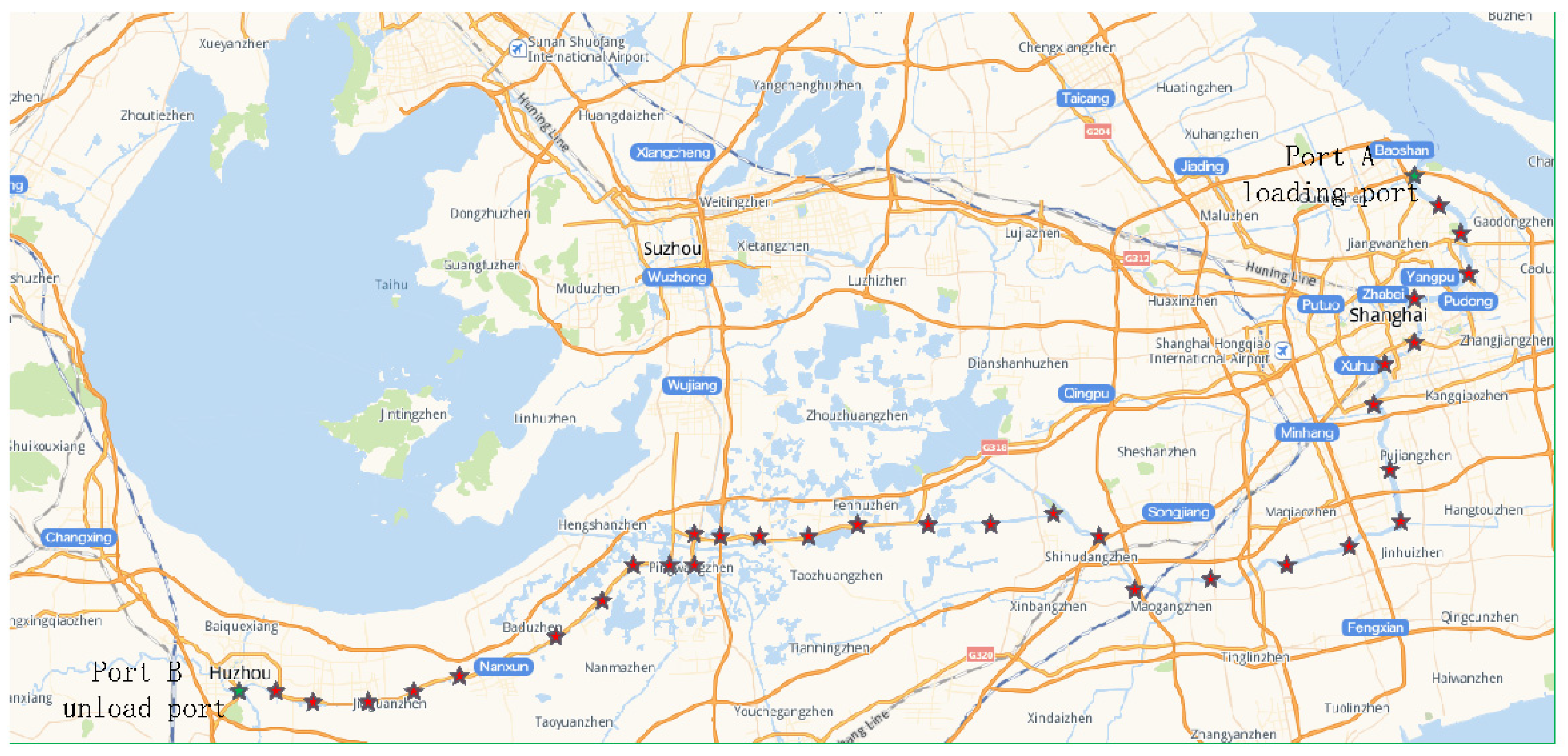
2.2. Ship Route Description

Though the battery-only powered ships do not need to consider how to plan their sailing route, for medium- and long-distance inland voyages, their entire route also can be divided into several segments according to the environmental factors of the waterway, such as the water depth, the water speed, and the tide. Without losing generality, we consider a battery-only powered ship route as shown in Figure 2. The energy management system of the battery-only powered ships must always pay attention to the SoC level of the battery groups in each route segment and adjust the ship sailing speed if it is necessary to guarantee the remaining battery energy can satisfy the energy demand for the remaining distance.

The whole voyage time $T_{wv}$ of the battery-only powered ships in a round trip can be denoted as,

$$T_{wv}=T_{hl}+T_{ll}+T_{ol}+T_{ul}+T_{rest}+T_c^A+T_c^B$$

(1)

where $T_{hl}$ is the sailing time of heavy load, $T_{ll}$ is the sailing time of light load, $T_{ol}$ is the loading time, $T_{ul}$ is the unloading time, $T_{rest}$ is the rest time between two consecutive voyages, $T_c^A$ is the battery charge time in port A, and $T_c^B$ is the battery charge time in port B.

Generally, $T_{ol}$, $T_{ul}$, and $T_{rest}$ are all considered as constant values for a given ship in the given route. $T_{hl}$, $T_{ll}$, $T_c^A$, and $T_c^B$ are auxiliary decision variables, which are used to help determine the optimal sailing speed of heavy load and light load statuses and the charged energy at the ports. They can be illustarted as the follows

$$T_{hl}={\displaystyle \sum }_{i=1}^N{T}_{hl,i}={\displaystyle \sum }_{i=1}^N\frac{D_{AB,i}}{V_{hl,i}}$$

(2)

$$T_{ll}={\displaystyle \sum }_{i=1}^N{T}_{ll,i}={\displaystyle \sum }_{i=1}^N\frac{D_{AB,i}}{V_{ll,i}}$$

(3)

where $N$ indicates the segment numbers, which means that the whole ship voyage is divided into N divisions. $i$ is the segment index. $T_{hl,i}$, $T_{ll,i}$ are the heavy load sailing and light load sailing in the $i\mathrm{th}$ segment, respectively. $V_{hl,i}$, $V_{ll,i}$ are the actual heavy and light load sailing speed to land in the $i\mathrm{th}$ segment, respectively. $D_{AB,i}$ is the distance of the $i\mathrm{th}$ segment.

Considering the waterway environment, the sailing speed to land can be described as follows. It is the combination of the ship sailing speed in calm water, the water speed, and the shallow water effect.

$$V_{hl,i}=V_{hlsw,i}-V_{hlswe,i}+V_{water,i}$$

(4)

$$V_{ll,i}=V_{llsw,i}-V_{llswe,i}+V_{water,i}$$

(5)

where $V_{hlsw,i}$, $V_{llsw,i}$ are the ship hydrostatic speeds of heavy load and light load in the $i\mathrm{th}$ segment, respectively. $V_{hlswe,i}$, $V_{llswe,i}$ are the shallow water effect of heavy load ship and light load ship in the $i\mathrm{th}$ segment, respectively. $V_{water,i}$ is the water speed in the $i\mathrm{th}$ route segment.

In Equations (4) and (5), $V_{water,i}$ is only determined by the environment and it has no relationship to the ship. The values of $V_{hlswe,i}$ and $V_{llswe,i}$ are determined by the ship shaft, the water depth, and the ship sailing speed. For a given ship, $V_{hlsw,i}$ and $V_{llsw,i}$ are only determined by the ship shaft power.

The battery charge times in port A and port B are shown in the follow

$$T_c^A=\frac{E_c^A}{P_c^A}$$

(6)

$$T_c^B=\frac{E_c^B}{P_c^B}$$

(7)

where $E_c^A$, $E_c^B$ are the absorbed energy of the ship in port A and port B, respectively. $P_c^A$ and $P_c^B$ are the charge power of the ship in port A and port B, respectively. No matter how much the electricity price is after the power charging at the ports, the left energy of the battery must satisfy the left distance used.

To meet the logistic requirement, the whole sailing time $T_{wv}$ must be less than a given time threshold.

$$T_{wv}\le T_{wv}^{max}$$

(8)

where $T_{wv}^{max}$ is the permitted maximum time consumption over a round trip. Generally, $T_{wv}^{max}$ is a given value.

3. Mathematical Modeling

This section provides the constraints and objective of the battery capacity optimization problem for a battery-only powered ship.

3.1. Ship Sailing Model

(1)

Ship sailing speed constraint

For a medium- and long-distance inland voyage, it may pass through a waterway with different administrative control and different navigation conditions, which leads to the permit-table ship sailing speed may be different. Therefore, the sailing plan of the battery-only powered ship must meet the speed constraint of the local district.

$$V_i^{min}\le V_{V_{hl,i}}\le V_i^{max}$$

(9)

$$V_i^{min}\le V_{ll,i}\le V_i^{max}$$

(10)

where $V_i^{min}$, $V_i^{max}$ are the permitted minimum ship sailing speed and maximum ship sailing speed.

(2)

Statistical model of shallow water effect

As is well known to all, when the river is not deep enough, the river bottom is close to the ship bottom, and the river will produce a counteraction to reduce the ship’s sailing. This counteraction is called the shallow water effect. The accurate shallow water effect model is very complex, and its modeling method cannot be easily grasped for a person without professional knowledge of ship designation. To describe the shallow water effect in a simple way, we use an approximated mathematical model based on the data which is supplied by the ship design institute. After many comparative analyses, we choose the polynomial-based statistical model to describe the shallow water effect.

$$V_{hlswe,i}=a_{hl,i}{V}_{hlsw,i}{}^3+b_{hl,i}{V}_{hlsw,i}{}^2+c_{hl,i}{V}_{hlsw,i}+d_{hl,i}$$

(11)

$$V_{llswe,i}=a_{ll,i}{V}_{llsw,i}{}^3+b_{ll,i}{V}_{llsw,i}{}^2+c_{ll,i}{V}_{llsw,i}+d_{ll,i}$$

(12)

where $a_{hl,i}$, $b_{hl,i}$, $c_{hl,i}$, and $d_{hl,i}$ indicate the shallow water effect coefficient in the ith segment when the ship is heavily loaded. Similarly, $a_{ll,i}$, $b_{ll,i}$, $c_{ll,i}$, and $d_{ll,i}$ indicate the shallow water effect coefficient when the ship is lightly loaded at the $i\mathrm{th}$ segment.

(3)

Statistical model of ship hydrostatic speed and battery output power

As is known to all, the ship’s hydrostatic speed determines the energy consumption for a given ship with a given loading status. It is the most important parameter in battery-power ship sailing speed optimization. Various kinds of literature have proven that the ship’s hydrostatic speed and shaft power have a cubic relation [5,32]. By analyzing the data supplied by the ship design institute, we assume the ship’s hydrostatic speed and the shaft power have the following relationship.

$$P_{ps}\left(V_{hlsw}\right)=a{v}_{wv}^w{V}_{hlsw}{}^3+b{v}_{wv}^w{V}_{hlsw}{}^2+c{v}_{wv}^w{V}_{hlsw}+d{v}_{wv}^w$$

(13)

$$P_{ps}\left(V_{llsw}\right)=a{v}_{llsw}{V}_{llsw}{}^3+b{v}_{llsw}{V}_{llsw}{}^2+c{v}_{llsw}{V}_{llsw}+d{v}_{llsw}$$

(14)

where $a{v}_{wv}^w$, $b{v}_{wv}^w$, $c{v}_{wv}^w$, and $d{v}_{wv}^w$ are the heavy load coefficient at hydrostatic speed $V_{hlsw}$ and loading weight $w$, and $a{v}_{llsw}$, $c{v}_{llsw}$, and $d{v}_{llsw}$ are the light load coefficient of hydrostatic speed $V_{llsw}$. $P_{ps}\left(V_{hlsw}\right)$ and $P_{ps}\left(V_{llsw}\right)$ are the propeller shaft powers when heavy load and light load, respectively.

After the shaft power is obtained, the power of battery output can be calculated by considering the efficiency of the reduction gearbox, propulsion motor, propulsion frequency converter, inverter, and converter.

$$P_{bat}\left(V_{hlsw}\right)=\frac{P_{ps}\left(V_{hlsw}\right)}{{\eta }_{hlsw}}+\frac{P_{costom}}{{\eta }_{costom}}$$

(15)

$$P_{bat}\left(V_{llsw}\right)=\frac{P_{ps}\left(V_{llsw}\right)}{{\eta }_{llsw}}+\frac{P_{costom}}{{\eta }_{costom}}$$

(16)

where ${\eta }_{hlsw}$, ${\eta }_{llsw}$ are the aggregated efficiency value of the devices from the propeller to the battery, which includes reduction gearbox efficiency, propulsion motor efficiency, propulsion frequency converter efficiency, and converter efficiency. $P_{costom}$ is the domestic load, ${\eta }_{costom}$ is the aggregated coefficient value of the devices from the domestic devices to the battery, which includes power network loss, inverter efficiency, and converter efficiency. $P_b\left(V_{hlsw}\right)$ and $P_b\left(V_{llsw}\right)$ are the battery output power at heavy load and light load, respectively.

(4)

Battery energy using model

According to Equations (2), (3) and (15), (16), the battery energy consumption under heavy load and light load cases can be shown the below

$$E_{using}\left(V_{hl}\right)={\displaystyle \sum }_{i=1}^N{\mathrm{T}}_{hl,i}{P}_{bat}\left(V_{hlsw,i}\right)+T_{ol}\frac{P_{costom}}{{\eta }_{costom}}$$

(17)

$$E_{using}\left(V_{ll}\right)={\displaystyle \sum }_{i=1}^N{\mathrm{T}}_{ll,i}{P}_{bat}\left(V_{llsw,i}\right)+T_{ul}\frac{P_{costom}}{{\eta }_{costom}}$$

(18)

where $P_{bat}\left(V_{hlsw,i}\right)$, $P_{bat}\left(V_{llsw,i}\right)$ are the battery output power at the $i\mathrm{th}$ segment, respectively. $E_{using}\left(V_{hl}\right)$, $E_{using}\left(V_{ll}\right)$ are the ship’s energy consumption in heavy load and light load, respectively.

The minimum battery capacity to meet the ship’s energy consumption for sailing the on distance is calculated.

$$E_{bat}^{min}\left(V_{zh}\right)=\frac{max\left(E_{using}\left(V_{hl}\right),E_{using}\left(V_{ll}\right)\right)}{DoD}$$

(19)

where $DoD$ is the depth of discharge of the battery.

Equation (19) indicates that the usable battery energy must be larger than the aggregated value of ship sailing, shipload waiting, and ship rest, whether the ship is in heavy load or light load.

In addition, the actual optimal battery energy capacity $E_{bat}$ should be larger than $E_{bat}^{min}\left(V_{zh}\right)$ and less than the maximum permittable value $E_{bat}^{max}$.

$$min\left(E_{bat}^{min}\left(V_{zh}\right)\right)\le E_{bat}\le E_{bat}^{max}$$

(20)

where $E_{bat}^{max}$ is determined by the combined value of the maximum battery deployable space and the maximum investment cost. $min\left(E_{bat}^{min}\left(V_{zh}\right)\right)$ is the battery capacity that the ship sails with the minimum permit-table speed in each segment.

(5)

Port energy charging model

When the ship leaves the port, the stored battery energy must be larger than the energy consumption of the ship to sails to the next port.

$$E_{using}\left(V_{ll}\right)\ge E_{chag}^B\ge max\left(0,E_{using}\left(V_{hl}\right)-\left(E_{bat}DoD-E_{using}\left(V_{ll}\right)\right)\right)$$

(21)

where $E_{bat}DoD$ denotes the maximum dischargeable energy and $E_{bat}DoD-E_{using}\left(V_{ll}\right)$ denotes the remaining usable energy when the ship reaches the loading port.

It should be noted that, in order to improve the battery consistency, it should be generally assumed that the ship battery is fully charged at the beginning of each navigation.

$$E_{chag}^A+E_{chag}^B=E_{using}\left(V_{hl}\right)+E_{using}\left(V_{ll}\right)$$

(22)

(6)

Battery using time model

The practical number of ship voyages within the battery cycle life is shown below

$$N_{hc}\left(V_{hl}\right)=min\left(N_{avag}{Y}_{bat},round\left(\frac{min\left(L_{bat}{T}_{hc},Y_{bat}\times 365\times 24\right)}{T_{hc}}\right)\right)$$

(23)

where $Y_{bat}$ is the battery calendar life, $T_{hc}$ is the time of a whole voyage, $N_{avag}$ is the average voyage times yearly, and $365\times 24$ represents the hours of one year. $round\left(\frac{min\left(L_{bat}{T}_{hc},Y_{bat}\times 365\times 24\right)}{T_{hc}}\right)$ is used to find the maximum permittable ship transportation time just considering the batteries capability within the battery’s lifetime.

3.2. Objective

3.2.1. Revenue of Ship Transportation

Revenue of shipload transportation can be expressed as the following

$$R_{bat}^{life}=S_{hc}{N}_{hc}\left(V_{hl}\right)$$

(24)

where $S_{hc}$ is the revenue of one voyage and $N_{hc}\left(V_{hl}\right)$ is the ship sailing times within the battery life.

3.2.2. Ship Running Cost

The ship running cost within the battery life is the aggregated value of the battery charging cost $C_{bat}^{chag}$ at both ports, the battery initial investment cost $C_{bat}^{pucs}$, and the personal salary cost $C_{man}$. It is expressed as the following

$$C_{bat}^{life}=C_{bat}^{chag}+C_{bat}^{pucs}+C_{man}$$

(25)

The battery charging cost $C_{bat}^{chag}$ can be further expressed as

$$C_{bat}^{chag}=\frac{E_{chag}^A{c}_{ele}\left(A\right)+E_{chag}^B{c}_{ele}\left(B\right)}{{\eta }_{chager}}$$

(26)

where $c_{ele}\left(A\right)$, $c_{ele}\left(B\right)$ are the battery charging costs at port A and port B, respectively. ${\eta }_{chager}$ is the efficiency of the charger.

The battery initial investment cost $C_{bat}^{pucs}$ can be further expressed as

$$C_{bat}^{pucs}=c_{bat}^{buy}{E}_{bat}$$

(27)

where $c_{bat}^{buy}$ is the battery’s unit capacity cost, $E_{bat}$ is the battery capacity.

The personal salary cost $C_{man}$ can be further expressed as

$$C_{man}=c_{man}^{oney}{N}_{man}$$

(28)

where $c_{man}^{oney}$ is the average one crew’s yearly wage and $N_{man}$ is the number of crew members that this ship must deploy according to the policy.

Therefore, the objective of the battery sizing problem considering energy management for a battery-only powered ship is

$$\max S_{bat}^{net}=R_{bat}^{life}-C_{bat}^{life}$$

(29)

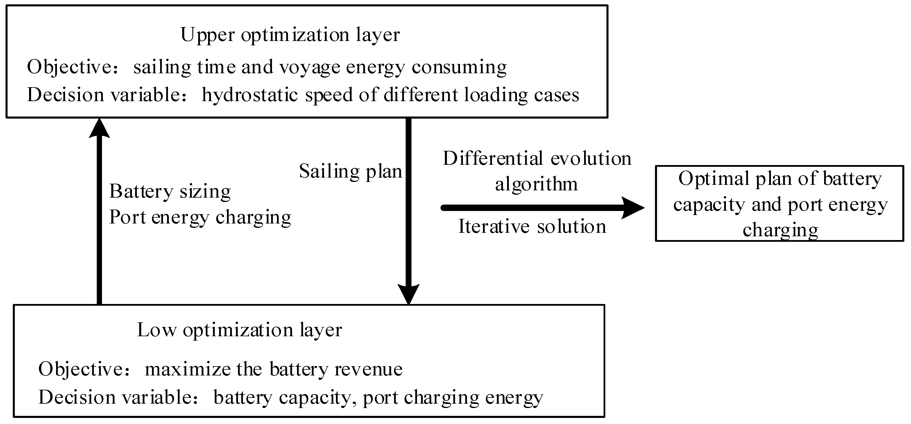
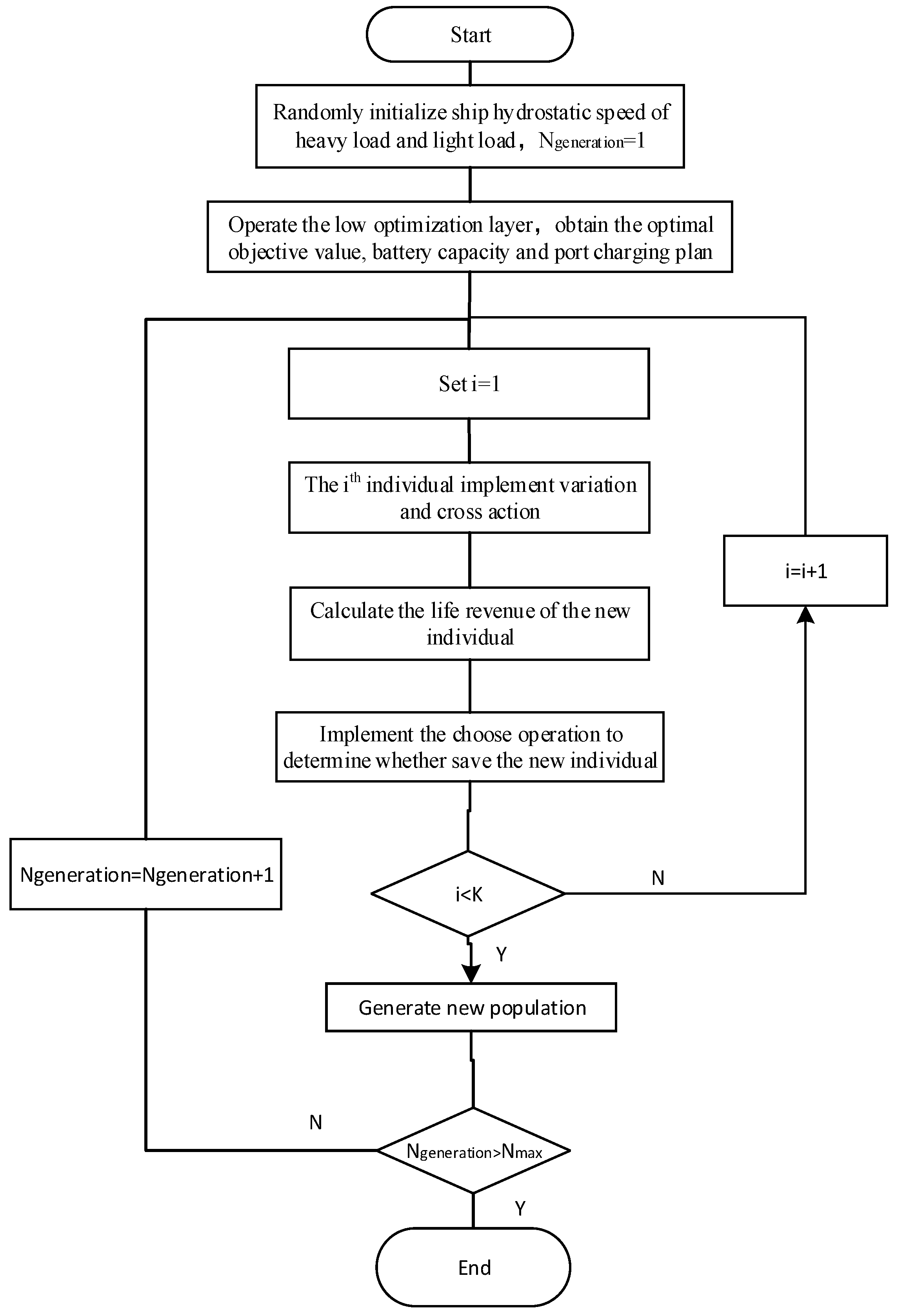
4. Optimization Algorithm

According to the modeling analysis of the previous section, the sailing time and energy consumption of the battery-powered ship are the nonlinear functions of the variables of sailing speed and battery initial size. Therefore, the joint optimization of the sailing speed and battery capacity is a multi-constraint and multi-variable nonlinear optimization problem. In order to decrease the solving complexity, the joint optimization problem is further divided into a bi-level optimization problem, as shown in Figure 3.

The upper optimization layer obtains many flexible ship sailing plans by implementing flexible, intelligent optimization algorithms, such as differential evolution algorithm, genetic algorithm, and particle swarm optimization algorithm. The ship sailing plans of the upper optimization layer will be imported to the lower optimization layer to obtain the optimal battery capacity and port energy-using plan. The upper and lower optimization layers update their results by the cross and variation actions until the end of the optimization.

Observing Figure 2, if the battery charging power at port A and port B is the fixed value, the lower optimization layer can be converted into a linear optimization problem from the main nonlinear optimization problem and greatly increase the solving efficiency.

Differential evolution (DE) proposed by Storn and Price in 1995 [33] is a population-based metaheuristic algorithm. Compared to other optimization algorithms, the DE algorithm needs few control parameters, is straightforward to implement, and it has a faster calculation speed and better global searchability. Therefore, the DE algorithm is adopted to solve the joint optimization model of the sailing speed and battery capacity in this paper. Its solving framework is shown below, where $K$ indicates the scale of the population and $N_{max}$ is the maximum iteration times of the proposed differential evolution algorithm.

In Figure 4, DE evolves the population by driving the mutation and selection operators [34]. The mutation has exploration ability with exploring different regions of the search space, while the selection has the exploitation ability with finding local optimal points.

5. Case Study and Results Analysis

5.1. Case Description

Two cases are discussed in this section. The first case has a medium–long distance route of about 270 km and has several segments, and the second case has a short distance route of about 100 km and only one segment. The above two cases are obtained from a constructing battery-power dry bulk carrier. The ship has a length of 62.8 m, a width of 12.4 m, a depth of 4 m, a design cargo capacity of 1600 tons, and a design sailing speed is 10 km/h.

Due to the limitation of the propulsion motor, the maximum hydrostatic speed of the ship is set as 14 km/h. After the calculation and simulation of the above-mentioned ship by the ship design institute, the ship’s shaft power at different hydrostatic speeds and loading states are shown in

Table 1. Design parameter of a battery-only powered inland water ship.

Ship Hydrostatic Speed (kW/h)	Full Load Sailing Power Demand (kW)	Light Load Sailing Power Demand (kW)
6.00	49.14	42.29
7.00	58.49	48.54
8.00	68.58	56.29
9.00	85.13	68.43
10.00	103.18	79.70
11.00	124.96	97.17
12.00	152.44	116.47
13.00	195.00	139.85
14.00	251.58	167.01

. Concurrently, the other parameters used in the case study are shown in

Table 2. Parameters of a battery-powered bulk freighter ship.

Parameters	Value
The minimum ship to land speed	3 kn
Ship loading time	3 h
Ship unloading time	3 h
Ship retiring time in the midway	2 h
Retiring time between the two navigations	12 h
Load transportation income	3 $/t
Manual cost	300 $/time/person
Battery discharge DoD	0.8
Battery calendar life	10 years
Battery cycling life	3000 times
Ship power demand when midway retiring	5 kW

, such as the minimum ship to land speed, ship loading and unloading time, battery discharge DoD, and so on. The ship navigation data were approved by many captains who have many years of experience in this route navigation and the battery data were collected from batteries approved by the China Classification Society (CCS).

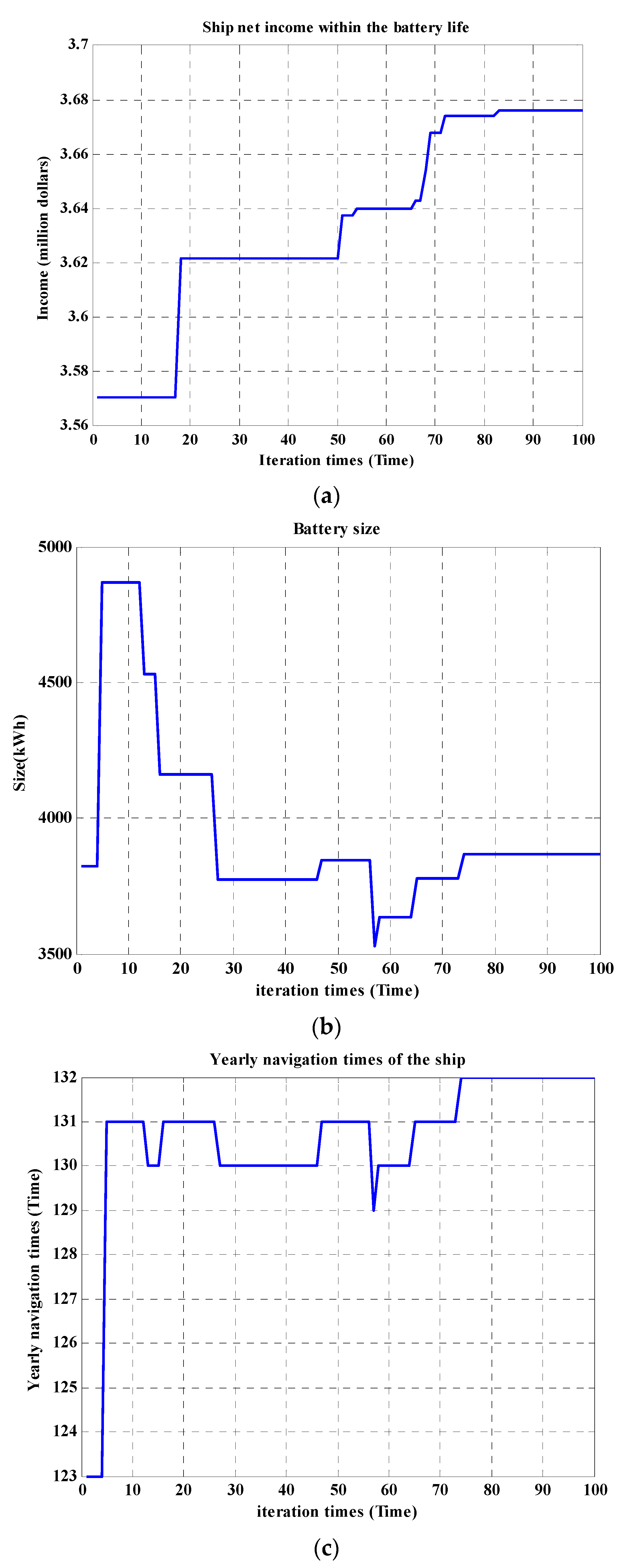
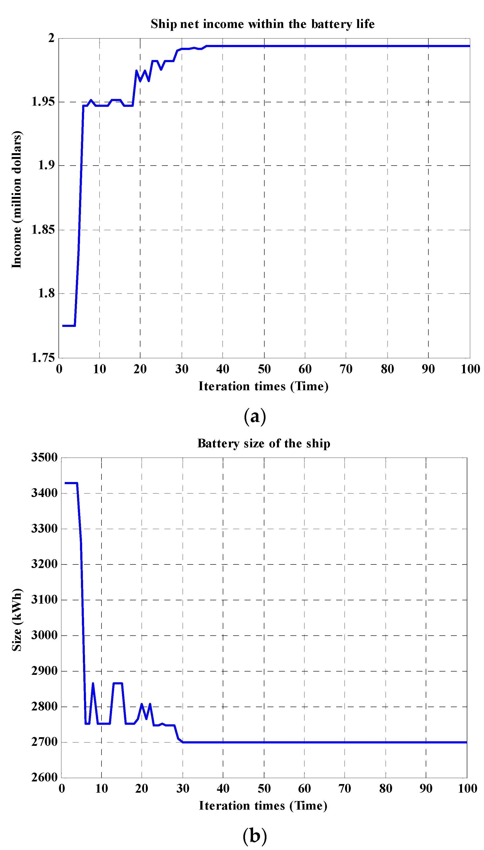
5.2. Case 1: Example of Medium-Long Route

In this case, the inland water transport route is from Taicang port located in Jiangsu Province to Huzhou port located in Zhejiang Province. The distance is 270 km, as shown in Figure 5. This route includes five types of water segments, as demonstrated in

Table 3. The voyage information of case 1.

Segment Number	Distance	Water Speed	Speed Limit
Segment 1	40 km	3 km/h	≥6 knots
Segment 2	6 km	−3 km/h	≥3 knots
Segment 3	56 km	3 km/h	≥4 knots
Segment 4	68 km	1 km/h	≥3 knots
Segment 5	24 km	0	≥3 knots
Segment 6	76 km	Has shallow water effect	≥3 knots

. They are the tide positive affected segment, the tide negative affected segment, the against the water segment, the still water segment, and the shallow water affected segment. The maximum time used for a voyage is set as 96 h, and the loading sailing time is set as 40 h.

The sailing and battery sizing optimization procedures are shown as follows:

Firstly, the fitting function between the battery output power and the ship’s hydrostatic speed is obtained by the polynomial fitting approach, considering the ship loading state.

Secondly, the fitting function between the shallow water effect value and the ship’s hydrostatic speed is also obtained by the polynomial fitting approach, considering the ship loading state.

Then, the proposed optimization method is applied to different utilization scenarios to verify its superiority, such as whether the load amount is sufficient or whether the port’s battery charging price is the same.

Scenario 1: electricity charging prices at port B and port A are the same, and the load is sufficient for the ship transportation.

In this scenario, the battery charging devices at port B and port A are both supported by the transport corporation and the district agency. Hence, the battery charging prices in these ports are both set as 0.06 $/kWh. In addition, there are large number of loads that need to be carried from port A to port B, so the ship can fully demonstrate its capability. The results as shown in Figure 6.

Figure 6 indicates the proposed optimization algorithm can effectively obtain the convergence solvation. The ship can achieve an income of 4.1779 million dollars over the battery’s life with yearly navigation of 132 times. This demonstrates that the battery’s cycle life is not fully utilized because only 2640 charge/discharge cycles are implemented over its 10 years calendar life. The optimal battery capacity is 3865.4 kWh, and the battery energy used sailing a fully loaded ship is 3075.4 kWh. Meanwhile, the battery energy used by a ship sailing with an empty load is 2678.9 kWh. The deployed battery capacity can just meet the full load required for sailing. In addition, the power charging principle at the two ports is the same, i.e., full charge before leaving. The sailing plan of the ship is shown in

Table 4. Sailing plan of the ship in one whole navigation.

Ship Hydrostatic Speed	Segment 1	Segment 2	Segment 3	Segment 4	Segment 5	Segment 6
Full load sailing	9.11	14	10	9.6	10	10
Empty load sailing	14	14	13.9	14	14	14

.

Table 4 indicates that the optimal ship sailing speed is much higher than its permitted minimum sailing speed and the empty load sailing speed is much higher than the full load speed. This indicates that the ship can effectively increase its income by raising its sailing speed, but the full load sailing power demand is very large and it increases sharply with the sailing speed. Hence, 10 km/h is the most suitable hydrostatic speed. On the other side, the empty load sailing power demand is not very large and it increases slowly to the full load condition. Hence, it can sail with the maximum speed to decrease the empty load sailing time.

Scenario 2: electricity charging price at port B is higher than port A, and the load is sufficient for the ship transportation.

In this case, the battery charging device at port A is supported by the port corporation, so its battery charging price is very high, namely set as 0.2 $/kWh. However, the battery charging device in port B is supported by the ship corporation and the district agency, so its battery charging price is low, usually 0.05 $/kWh. Similar to Scenario 1, a large number of loads need to be carried from port A to port B, so the ship can fully demonstrate its capability. The results are shown in Figure 7.

Figure 7 indicates that the proposed optimization algorithm can effectively obtain the convergence solvation. The ship can achieve an income of 3.676 million dollars over the battery’s life with yearly navigation of 128 times. Similar to scenario 1, the battery’s cycle life is not fully utilized, because only 2560 charge/discharge cycles are implemented over its 10 years calendar life. The optimal battery capacity is 3390.4 kWh, and the battery energy used by a ship sailing with a full load is 2695.3 kWh. Meanwhile, the battery energy used by a ship sailing with an empty load is 2541.6 kWh. The deployed battery capacity can just meet the requirements for full load sailing and the battery is chosen to charge fully at both ports. The sailing plan of the ship is shown in

Table 5. Sailing plan of the ship in one whole navigation.

Ship Hydrostatic Speed	Segment 1	Segment 2	Segment 3	Segment 4	Segment 5	Segment 6
Full load sailing	9.11	10.4	8	9.3	10	9.1
Empty load sailing	11	14	13.9	14	13	14

.

Compared to Table 4, the ship’s full load and empty load sailing speeds are both slowed to reduce the battery size demand and offset the negative impacts of the high electricity charging cost in port B.

Scenario 3: The electricity charging price at port B is equal to port A, but the load is insufficient.

In this scenario, the battery charging devices at port B and port A are the same and are both set as 0.06 $/kWh. However, the port does not have a sufficient load to provide the ship to carry. The maximum yearly navigation time is only 70. The results as shown in Figure 8.

In Figure 8, the ship can achieve an income of 2.12 million dollars over the battery’s life with yearly navigation of 70 times. In this scenario, the battery’s cycle life cannnot be fully utilized, because only 1400 charge/discharge cycles are implemented over its 10 year calendar life. The optimal battery capacity is 2689.6 kWh, and the battery energy used by a ship sailing with a full load is 2141.9 kWh. Meanwhile, the battery energy used by a ship sailing with an empty load is 2139 kWh. The deployed battery capacity can just meet the full load sailing requirement and the battery is chosen to charge fully at both ports. The sailing plan of the ship is shown in

Table 6. Sailing plan of the ship in one whole navigation.

Ship Hydrostatic Speed	Segment 1	Segment 2	Segment 3	Segment 4	Segment 5	Segment 6
Full load sailing	8.11	10.4	6	6	7	6
Empty load sailing	8.1	14	14	6	14	14

.

Compared to Table 4, the ship full load sailing speed slowed much. Correspondingly, the battery size demand was reduced significantly. In addition, due to the load demand being fixed, there is no need to reduce the navigation time. Hence, the empty load sailing speed is also reduced much.

Scenario 4: The electricity charging price at port B is higher than port A, but the load is insufficient.

In this scenario, the battery charging device at port B is 0.2 $/kWh, and 0.06 $/kWh at port A. In addition, the port does not have a sufficient load to provide the ship to carry. The maximum yearly navigation time is only 70. The results as shown in Figure 9.

In Figure 9, the ship can achieve an income of 1.994 million dollars over the battery’s life with yearly navigation of 70 times. The income decreased is due to the high battery charge cost in port A. Similar to Scenario 3, the battery’s cycle life cannnot be fully utilized because only 1400 charge/discharge cycles are implemented over its 10 years cal life. The optimal battery capacity is 2698.6 kWh, and the battery energy used by a ship sailling with a full load is 2141.9 kWh. Meanwhile, the battery energy used by a ship sailing with an empty load is 1250.7 kWh. The deployed battery capacity can just meet the full load sailing requirement and the battery is both chosen to charge fully at the two ports. The sailing plan of the ship is shown in

Table 7. Sailing plan of the ship in one whole navigation.

Ship Hydrostatic Speed	Segment 1	Segment 2	Segment 3	Segment 4	Segment 5	Segment 6
Full load sailing	8.11	10.4	6	6	7	6
Empty load sailing	8.1	10.4	6	7	6	6

.

Compared to Table 5, it can be found that comparing the load demand between the ports, the impacts of port electricity cost can be negligible.

According to the analysis of the above scenarios of Case 1, it can be found that if the load demand is sufficient, the ship should try its best to increase the navigation times to achieve the maximum profit. The ship full load sailing speed is near its design speed and the battery calendar life is the restricted limit to further the ship’s profit. If the battery purchasing cost is fixed, the maximum navigation time is mainly determined by the electricity price of the loading port. The lower battery size, the higher the electricity price. However, if the load demand is insufficient, no matter what the port electricity price is, the deployed battery only satisfies the minimum sailing speed energy consumption to maximize the transportation revenue.

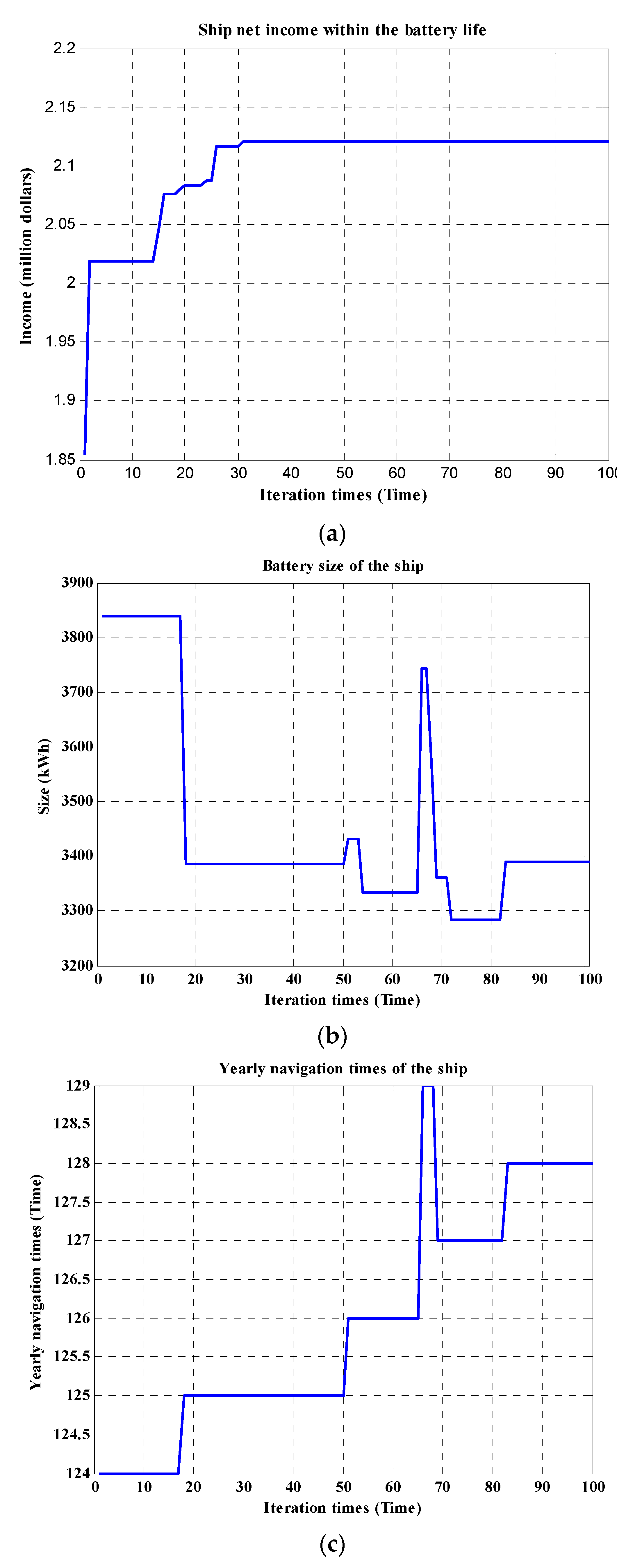
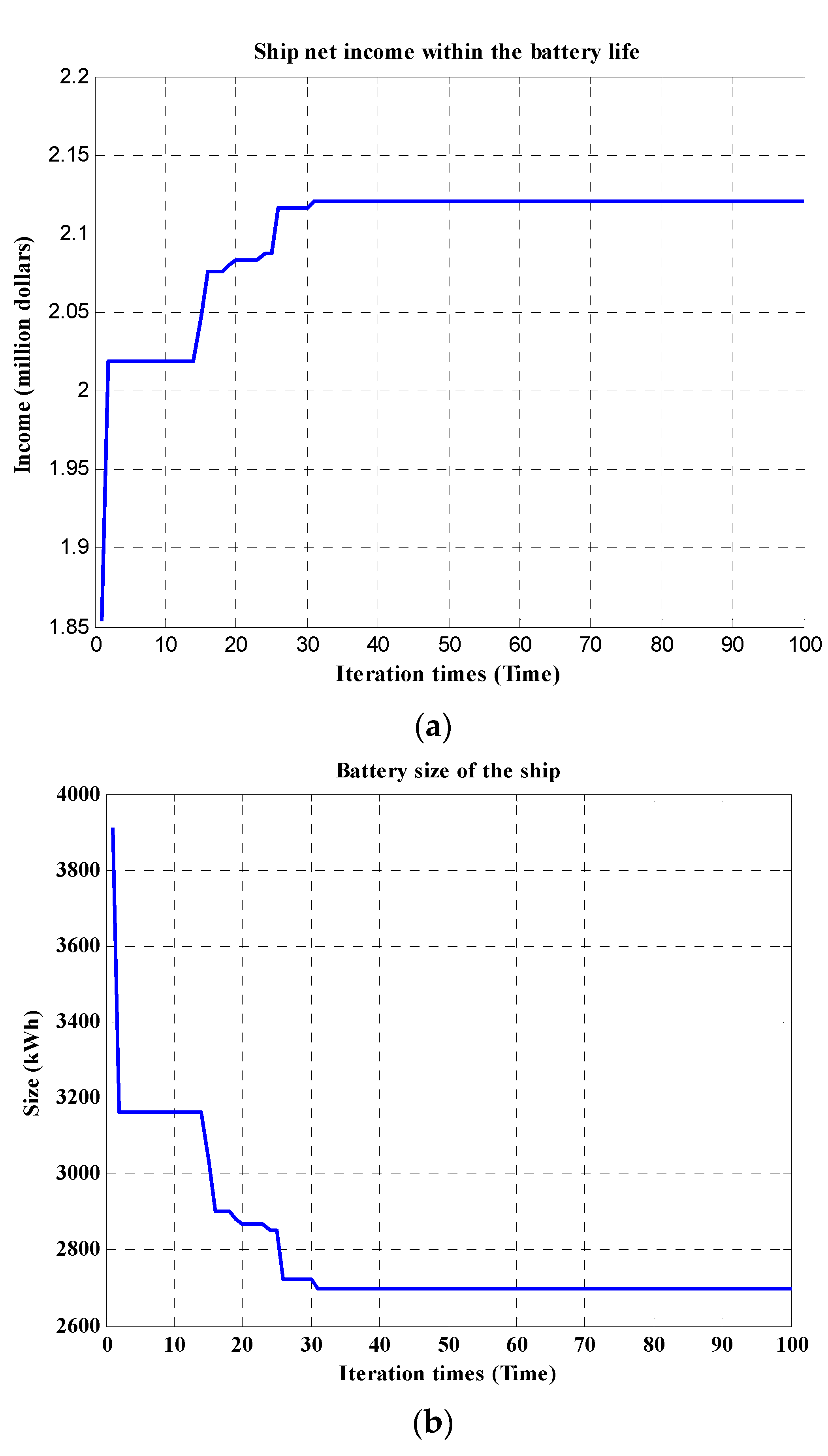
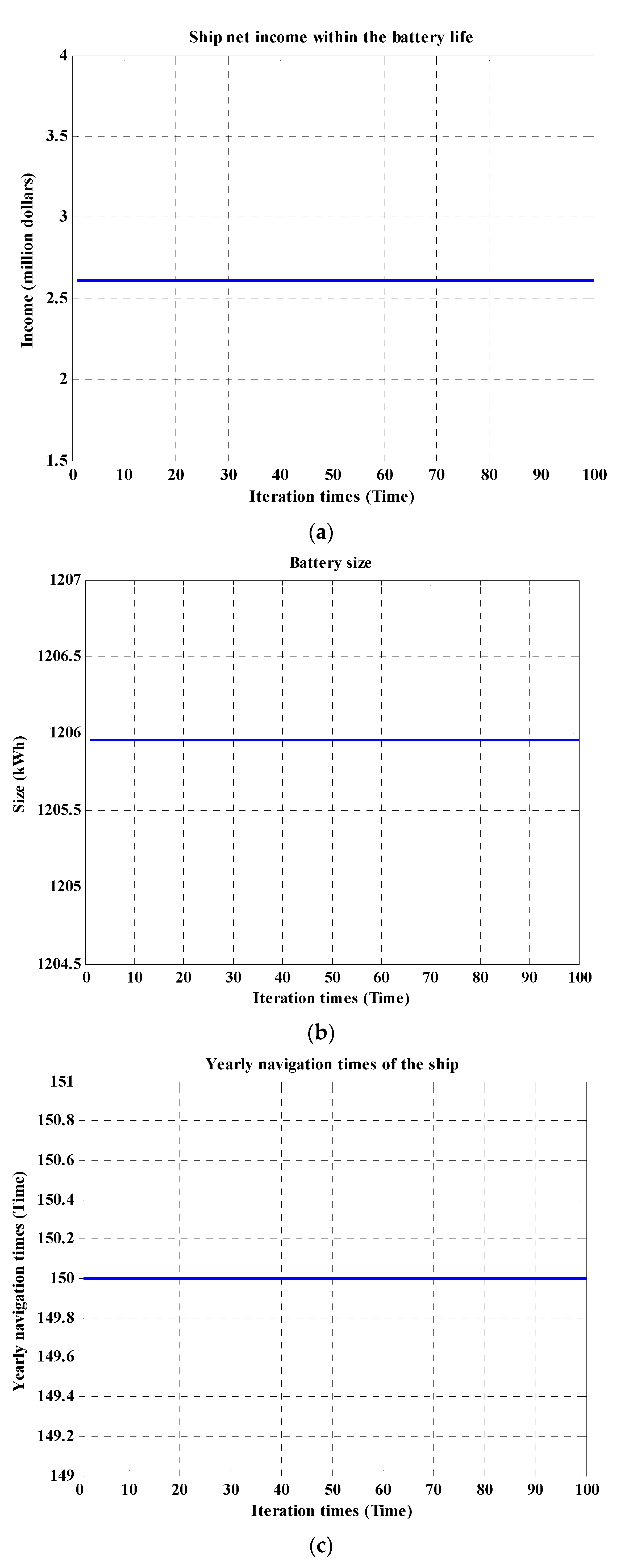
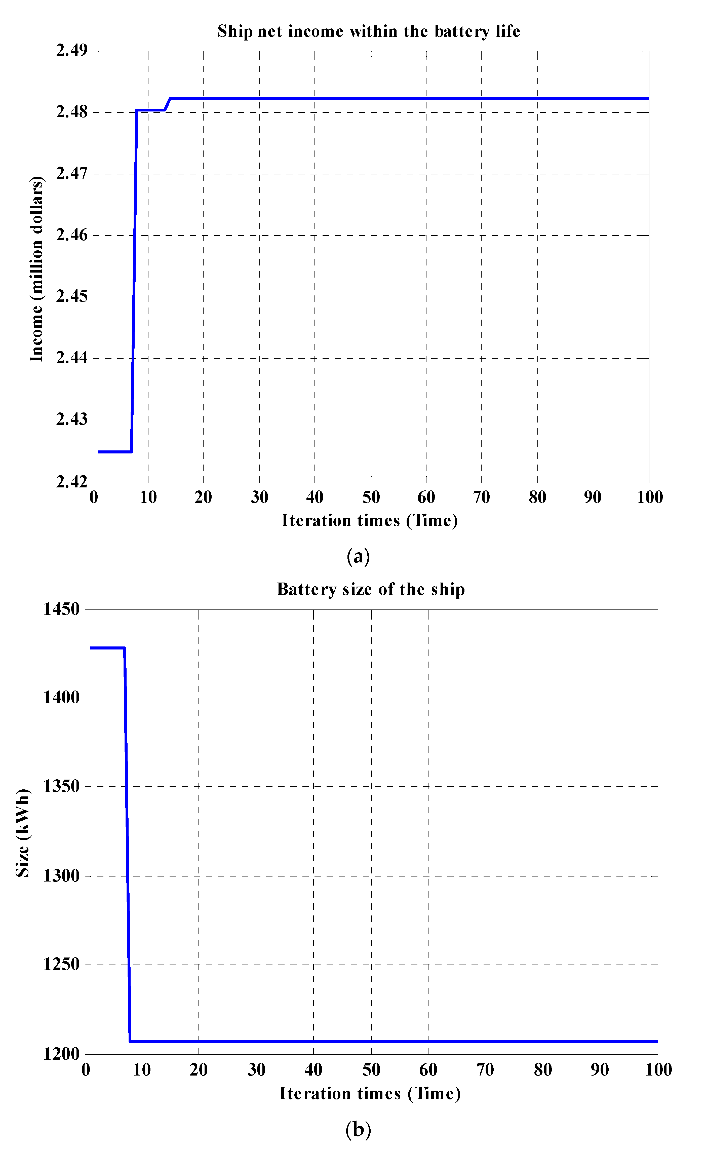
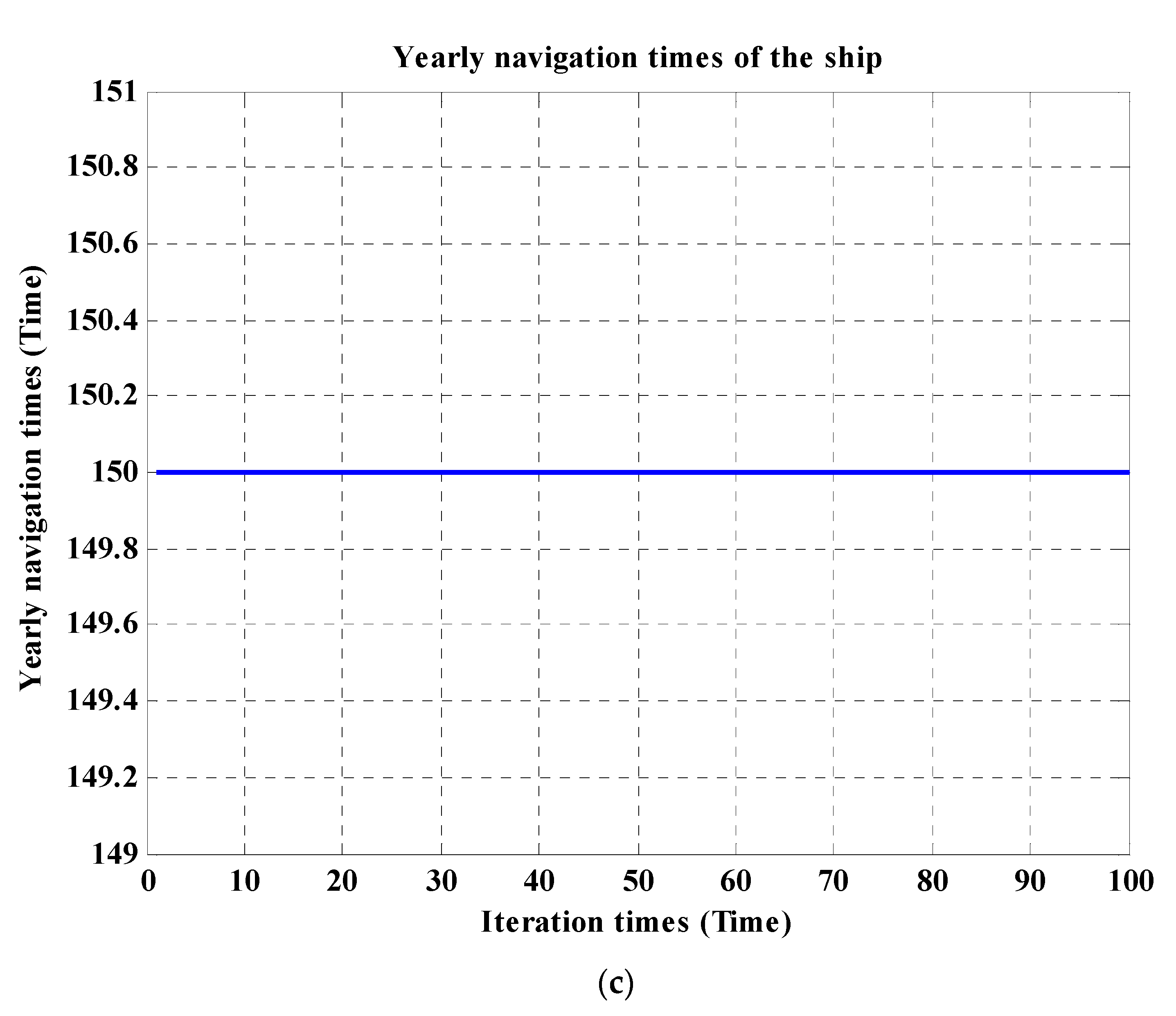
5.3. Case 2: Example of Near Route

In this case, the inland water transport route is just in Zhejiang Province, from Huzhou port to Jiaxing port. The distance is 100 km. This route only includes one type of water segment, this segment has been affected by the shallow water effect. The maximum time used for a voyage is set as 72 h, and the loading sailing time is set as 20 h. The load transportation income is 2 $/t and the manual cost is 100 $/time/person. The battery parameters and ship sailing parameters are shown in Table 2. Similar to Case 1, four scenarios are discussed.

Scenario 1: electricity charging prices at port B and port A are the same, and the load is sufficient for the ship transportation.

In this scenario, the battery charging cost at port A and port B are the same, namely 0.05 $/kWh. In addition, the load at port A is sufficient as it can support the ship carrying as its maximum capability.

Figure 10 indicates the proposed optimization algorithm can effectively obtain the convergence solvation for Case 2, and the convergency speed is very fast. The ship can achieve an income of 2.61 million dollars over the battery’s life with yearly navigation of 150 times. Due to the navigation distance is not far, the battery’s cycling life is fully used over its clander life. The optimal battery capacity is 1206 kWh, and the battery energy used by a ship sailing with a full load is 947.4 kWh. Meanwhile, the battery energy energy used by a ship sailing with an empty load is 932.5 kWh. The deployed battery capacity can just meet the full load sailing requirement and the battery is chosen to charge fully at both ports. The full load sailing speed is 6.2 km/h and the empty load sailing speed is 12.1 km/h.

Scenario 2: electricity charging price at port B is higher than port A, and the load is sufficient for the ship transportation.

In this scenario, the battery charging device at port A is higher than port B, which is 0.2 $/kWh for port A and 0.05 $/kWh for port B. Similar to Scenario 1, there are a large number of loads that need to be carried from port A to port B, so the ship can fully demonstrate its capability.

In Figure 11, the ship can achieve an income of 2.48 million dollars over the battery’s cycling life with yearly navigation of 150 times. Similar to scenario 1, the battery’s cycle life is fully used. The optimal battery capacity is 1207 kWh, and the battery energy used by a ship sailing with a full load is 948.5 kWh. Meanwhile, the battery energy energy used by a ship sailing with an empty load is 566.9 kWh. The deployed battery capacity can just meet the full load sailing requirement and the battery is chosen to charge fully at both ports. Due to the high charging cost of port A, the ship’s empty load sailing speed is slow compared to scenario 1. The full load sailing speed is 6.2 km/h and the empty load sailing speed is 6.1 km/h.

Scenario 3: electricity charging price at port B is equal to port A, and the load is insufficient for the ship transportation.

In this scenario, the battery charging device at port A and port B are the same, they both are 0.05 $/kWh. However, the load at port A is not enough, it only can support a yearly variation of 100 navigation times.

In Figure 12, the ship can achieve an income of 1.66 million dollars over the battery’s cycling life with yearly navigation of 100 times. The optimal battery capacity is 1205.4 kWh, and the battery energy used by a ship sailing with a full load is 948.5 kWh. Meanwhile, the battery energy used by a ship sailing with an empty load is 567.0 kWh. The deployed battery capacity can just meet the full load sailing requirement and the battery is chosen to charge fully at both ports. Due to the low charging cost of port A, the ship’s empty load sailing speed is fast compared to the full load state. The full load sailing speed is 6.2 km/h and the empty load sailing speed is 6 km/h.

Scenario 4: The electricity charging price at port B is higher than port A, and the load is insufficient.

In this scenario, the battery charging cost at port A is 0.2 $/kWh and it is 0.05 $/kWh at port B. In addition, the load at port A is not enough, it only can support a yearly variation of 100 navigation times.

In Figure 13, the ship can achieve an income of 1.658 million dollars over the battery’s cycling life with yearly navigation of 100 times. The optimal battery capacity is 1216 kWh, and the battery energy used by a ship sailing with a full load is 948.5 kWh. Meanwhile, the battery energy used by a ship sailing with an empty load is 955.7 kWh. The deployed battery capacity can just meet the full load sailing requirement and the battery is chosen to charge fully at both ports. To save cost, the ship’s empty load sailing speed is also very low. The full load sailing speed is 6 km/h and the empty load sailing speed is 12.3 km/h.

According to the analysis of the above scenarios of Case 2, it can be found that due to the voyage distance not being very long, the cycling using times becomes the restricted limit to further maximize the ship’s revenue if the load demand is sufficient. Because the ship’s full load sailing speed is its minimum permittable speed in this case, the battery capacity cannot be further optimized.

6. Conclusions

This paper proposes a joint optimization of battery size and ship sailing speed for a battery-powered all-electric inland dry bulk ship to maximize the ship’s life revenue. This ship can only charge power at its start port, and due to the complexity of the navigation waterway, it can be divided into several different segments with different environmental conditions. A joint optimization of battery size and ship sailing speed model is established considering the ship sailing speed constraint, the approximated shallow water effect model, the approximated relationship model of ship hydrostatic speed and battery output power, the battery energy using the model, and the port energy charging model. To solve this multi-variable nonlinear optimization problem, a bi-level optimization framework is implemented to decompose the solution complexity. Then, the differential evolution algorithm is used to obtain the final results. Two case studies with eight scenarios are analyzed. The results indicate that the proposed method can provide a suitable sailing speed considering the waterway environment and adjust it when the input parameters are changed. If the battery purchase cost is fixed, no matter how far the distance is, the load demand between the ports has the most impact on the ship’s battery capacity and sailing speed. Meanwhile, the port electricity charging cost has important effects on the ship’s battery capacity. The navigation distance changes the impact of battery sizing and the ship sailing speed is changed correspondingly. Though battery-powered ship investment is very sensitive, the proposed method can always find the optimal battery capacity and ship sailing speed plan.

In the future, we will focus on studying the best battery deployment plan for a battery-powered ship program with several ships.

References

1. Sundvor, I.; Thorne, R.J.; Danebergs, J.; Aarskog, F.; Weber, C. Estimating the replacement potential of Norwegian high-speed passenger vessels with zero-emission solutions. Transp. Res. Part D Transp. Environ. 2021, 99, 103019. [Google Scholar] [CrossRef]
2. Gaber, M.; El-Banna, S.; El-Dabah, M.; Hamad, M. Intelligent Energy Management System for an all-electric ship based on adaptive neuro-fuzzy inference system. Energy Rep. 2021, 7, 7989–7998. [Google Scholar] [CrossRef]
3. Fan, A.; Wang, J.; He, Y.; Perčić, M.; Vladimir, N.; Yang, L. Decarbonising inland ship power system: Alternative solution and assessment method. Energy 2021, 226, 120266. [Google Scholar] [CrossRef]
4. Kim, K.; Park, K.; Lee, J.; Chun, K.; Lee, S.-H. Analysis of Battery/Generator Hybrid Container Ship for CO2 Reduction. IEEE Access 2018, 6, 14537–14543. [Google Scholar] [CrossRef]
5. Kanellos, F.D. Optimal Power Management With GHG Emissions Limitation in All-Electric Ship Power Systems Comprising Energy Storage Systems. IEEE Trans. Power Syst. 2014, 29, 330–339. [Google Scholar] [CrossRef]
6. Wen, S.; Zhao, T.; Tang, Y.; Xu, Y.; Zhu, M.; Fang, S.; Ding, Z. Coordinated Optimal Energy Management and Voyage Scheduling for All-Electric Ships Based on Predicted Shore-Side Electricity Price. IEEE Trans. Ind. Appl. 2021, 57, 139–148. [Google Scholar] [CrossRef]
7. Weiming, M. Development of vessel integrated power system. In Proceedings of the 2011 International Conference on Electrical Machines and Systems (ICEMS), Beijing, China, 20–23 August 2011; pp. 1–6. [Google Scholar] [CrossRef]
8. Weiming, M. A survey of the second-generation vessel integrated power system. In Proceedings of the 2011 The International Conference on Advanced Power System Automation and Protection, Beijing, China, 16–20 October 2011; pp. 107–114. [Google Scholar] [CrossRef]
9. Kim, S.-Y.; Choe, S.; Ko, S.; Sul, S.-K. A Naval Integrated Power System with a Battery Energy Storage System: Fuel efficiency, reliability, and quality of power. IEEE Electrif. Mag. 2015, 3, 22–33. [Google Scholar] [CrossRef]
10. Huang, M.; He, W.; Incecik, A.; Cichon, A.; Królczyk, G.; Li, Z. Renewable energy storage and sustainable design of hybrid energy powered ships: A case study. J. Energy Storage 2021, 43, 103266. [Google Scholar] [CrossRef]
11. Diab, F.; Lan, H.; Ali, S. Novel comparison study between the hybrid renewable energy systems on land and on ship. Renew. Sustain. Energy Rev. 2016, 63, 452–463. [Google Scholar] [CrossRef]
12. Tang, R.; Li, X.; Lai, J. A novel optimal energy-management strategy for a maritime hybrid energy system based on large-scale global optimization. Appl. Energy 2018, 228, 254–264. [Google Scholar] [CrossRef]
13. Fang, S.; Xu, Y.; Wen, S.; Zhao, T.; Wang, H.; Liu, L. Data-Driven Robust Coordination of Generation and Demand-Side in Photovoltaic Integrated All-Electric Ship Microgrids. IEEE Trans. Power Syst. 2019, 35, 1783–1795. [Google Scholar] [CrossRef]
14. Lan, H.; Wen, S.; Hong, Y.-Y.; Yu, D.C.; Zhang, L. Optimal sizing of hybrid PV/diesel/battery in ship power system. Appl. Energy 2015, 158, 26–34. [Google Scholar] [CrossRef] [Green Version]
15. Qiu, Y.; Yuan, C.; Tang, J.; Tang, X. Techno-economic analysis of PV systems integrated into ship power grid: A case study. Energy Convers. Manag. 2019, 198, 111925. [Google Scholar] [CrossRef]
16. Zamani, M.A.; Sidhu, T.S.; Yazdani, A. Investigations Into the Control and Protection of an Existing Distribution Network to Operate as a Microgrid: A Case Study. IEEE Trans. Ind. Electron. 2013, 61, 1904–1915. [Google Scholar] [CrossRef]
17. Guerrero, J.M.; Chandorkar, M.; Lee, T.-L.; Loh, P.C. Advanced Control Architectures for Intelligent Microgrids—Part I: Decentralized and Hierarchical Control. IEEE Trans. Ind. Electron. 2013, 60, 1254–1262. [Google Scholar] [CrossRef] [Green Version]
18. Majumder, R. Reactive Power Compensation in Single-Phase Operation of Microgrid. IEEE Trans. Ind. Electron. 2012, 60, 1403–1416. [Google Scholar] [CrossRef]
19. Kumar Nunna, H.S.V.S.; Doolla, S. Multiagent-Based Distributed-Energy-Resource Management for Intelligent Microgrids. IEEE Trans. Ind. Electron. 2012, 60, 1678–1687. [Google Scholar] [CrossRef]
20. Jin, Z.; Meng, L.; Guerrero, J.M.; Han, R. Hierarchical Control Design for a Shipboard Power System With DC Distribution and Energy Storage Aboard Future More-Electric Ships. IEEE Trans. Ind. Inform. 2018, 14, 703–714. [Google Scholar] [CrossRef] [Green Version]
21. Faddel, S.; Saad, A.A.; Youssef, T.; Mohammed, O. Decentralized Control Algorithm for the Hybrid Energy Storage of Shipboard Power System. IEEE J. Emerg. Sel. Top. Power Electron. 2019, 8, 720–731. [Google Scholar] [CrossRef]
22. Hou, J.; Sun, J.; Hofmann, H. Control development and performance evaluation for battery/flywheel hybrid energy storage solutions to mitigate load fluctuations in all-electric ship propulsion systems. Appl. Energy 2018, 212, 919–930. [Google Scholar] [CrossRef]
23. Fagerholt, K.; Laporte, G.; Norstad, I. Reducing fuel emissions by optimizing speed on shipping routes. J. Oper. Res. Soc. 2010, 61, 523–529. [Google Scholar] [CrossRef]
24. Yuan, Z.; Liu, J.; Liu, Y.; Yuan, Y.; Zhang, Q.; Li, Z. Fitting Analysis of Inland Ship Fuel Consumption Considering Navigation Status and Environmental Factors. IEEE Access 2020, 8, 187441–187454. [Google Scholar] [CrossRef]
25. Xiong, Y.; Wang, Z.; Zhang, Y.; Yang, Y. Study on Route and Scheduling Optimization of Inland River Container Liner Ship Based on Interval Number Programming. In Proceedings of the 5th International Conference on Transportation Information and Safety, Liverpool, UK, 14–17 July 2019. [Google Scholar] [CrossRef]
26. Wang, K.; Li, J.; Huang, L.; Ma, R.; Jiang, X.; Yuan, Y.; Mwero, N.A.; Negenborn, R.R.; Sun, P.; Yan, X. A novel method for joint optimization of the sailing route and speed considering multiple environmental factors for more energy efficient shipping. Ocean Eng. 2020, 216, 107591. [Google Scholar] [CrossRef]
27. Belmonte, B.D.B.; Rinderknecht, S. Optimization Approach for Long-Term Planning of Charging Infrastructure for Fixed-Route Transportation Systems. World Electr. Veh. J. 2021, 12, 258. [Google Scholar] [CrossRef]
28. Hou, H.; Tang, J.; Zhao, B.; Zhang, L.; Wang, Y.; Xie, C. Optimal Planning of Electric Vehicle Charging Station Considering Mutual Benefit of Users and Power Grid. World Electr. Veh. J. 2021, 12, 244. [Google Scholar] [CrossRef]
29. Bao, X.; Xu, X.; Zhang, Y.; Xiong, Y.; Shang, C. Optimal Sizing of Battery Energy Storage System in a Shipboard Power System with considering Energy Management Optimization. Discret. Dyn. Nat. Soc. 2021, 2021, 2206. [Google Scholar] [CrossRef]
30. Othman, M.; Anvari-Moghaddam, A.; Ahamad, N.; Chun-Lien, S.; Guerrero, J.M. Scheduling of power generation in hybrid shipboard microgrids with energy storage systems. In Proceedings of the 2018 IEEE International Conference on Environment and Electrical Engineering and 2018 IEEE Industrial and Commercial Power System Europe (EEEIC/I&CPS Europe), Palermo, Italy, 12–15 June 2018; pp. 304–310. [Google Scholar] [CrossRef] [Green Version]
31. Wang, H.; Boulougouris, E.; Theotokatos, G.; Zhou, P.; Priftis, A.; Shi, G. Life cycle analysis and cost assessment of a battery powered ferry. Ocean Eng. 2021, 241, 110029. [Google Scholar] [CrossRef]
32. Buchem, M.; Golak, J.A.P.; Grigoriev, A. Vessel velocity decisions in inland waterway transportation under uncertainty. Eur. J. Oper. Res. 2021, 296, 669–678. [Google Scholar] [CrossRef]
33. Storn, R.; Price, K. Differential evolution–A simple and efficient heuristic for global optimization over continuous spaces. J. Glob. Optim. 1997, 11, 341–359. [Google Scholar] [CrossRef]
34. Das, S.; Suganthan, P.N. Differential Evolution: A Survey of the State-of-the-Art. IEEE Trans. Evol. Comput. 2011, 15, 4–31. [Google Scholar] [CrossRef]
Figure 1. Generic diagram of a battery-only power IPS.
Wevj 13 00040 g001
Figure 2. Illustration of a medium- and long-distance inland voyage.
Wevj 13 00040 g002
Figure 3. Bi-level optimization model of battery capacity determination for a battery-only powered ship.
Wevj 13 00040 g003
Figure 4. Solving framework of the proposed differential evolution algorithm.
Wevj 13 00040 g004
Figure 5. The inland water transport route of case 1.
Wevj 13 00040 g005
Figure 6. Simulation results of scenario 1 in case 1. (a) Variation of ship net income within the battery life over the optimization procedure (b) Battery capacity variation over the optimization procedure (c) Variation of yearly navigations over the optimization procedure.
Wevj 13 00040 g006
Figure 7. Simulation results of scenario 2 in case 1. (a) Variation of ship net income within the battery life over the optimization procedure (b) Battery capacity variation over the optimization procedure (c) Variation of yearly navigations over the optimization procedure.
Wevj 13 00040 g007
Figure 8. Simulation results of scenario 3 in case 1. (a) Variation of ship net income within the battery life over the optimization procedure (b) Battery capacity variation over the optimization procedure.
Wevj 13 00040 g008
Figure 9. Simulation results of scenario 4 in case 1. (a) Variation of ship net income within the battery life over the optimization procedure (b) Battery capacity variation over the optimization procedure.
Wevj 13 00040 g009
Figure 10. Simulation results of scenario 1 in case 2. (a) Variation of ship net income within the battery life over the optimization procedure. (b) Battery capacity variation over the optimization procedure. (c) variation of yearly navigations over the optimization procedure.
Wevj 13 00040 g010
Figure 11. Simulation results of scenario 2 in case 2. (a) Variation of ship net income within the battery life over the optimization procedure (b) Battery capacity variation over the optimization procedure (c) variation of yearly navigations over the optimization procedure.
Wevj 13 00040 g011aWevj 13 00040 g011b
Figure 12. Simulation results of scenario 2 in case 2. (a) Variation of ship net income within the battery life over the optimization procedure (b) Battery capacity variation over the optimization procedure.
Wevj 13 00040 g012
Figure 13. Simulation results of scenario 2 in case 2. (a) Variation of ship net income within the battery life over the optimization procedure (b) Battery capacity variation over the optimization procedure.
Wevj 13 00040 g013