Abstract
The purpose of this research is to develop a representative driving cycle for fuel cell logistics vehicles running on the roads of Guangdong Province for subsequent energy management research and control system optimization. Firstly, we collected and preliminarily screened the 42-day driving data of a logistics vehicle through the remote monitoring platform, and determined the vehicle characteristic signal vector for analysis. Secondly, the principal component analysis method is used to reduce the dimensionality of these characteristic parameters, avoiding the linear correlation between them and increase the comprehensiveness of the upcoming clustering. Next, the dimensionality-reduced data are fed to a clustering machine. K-means clustering method is used to gather the segmented road sections into highway, urban road, national highway and others. Finally, several segments are chosen in accordance to the occurrence possibility of the four types of road conditions, minimizing the deviation with the original data. By joining the segments and using a moving average filtering window, a typical driving cycle for this fuel cell logistics vehicle on a fixed route is constructed. Some statistical methods are done to validate the driving cycle.The effectiveness analysis shows the driving cycle we constructed has a high degree of overlap with the original data. This positive result provides a solid foundation for our follow-up research, and we can also apply this method to develop other urban driving cycles of fuel cell logistics vehicle.
1. Introduction
Fuel cell power system attracts much attention due to its high efficiency, high specific energy and environmental friendliness [1,2]. In recent years, several well-known automakers have turned their attention to fuel cells and launched corresponding fuel cell vehicles, such as Toyota’s Mirai, Honda’s Clarity, Hyundai’s nexo, and Mercedes-Benz’s GLC F-Cell. The governments of many countries and regions in the world have launched a series of policies to support the development of this industry and encourage the development of hydrogen refueling stations [3]. Commercial vehicles like logistics vehicles are considered to be the perfect candidates for promoting the industrialization of fuel cell vehicles, because usually they drive on a more structured and fixed route. Driving cycle is the basis of optimizing or validating test methods for energy consumption and emission of vehicles [4,5].
The driving cycle of fuel cell vehicles have a very important impact on the development of fuel cell systems. F. Nandjou et al. [6] studied the dynamic process of inlet gas heat and water transfer under NEDC for fuel cell performance. S. Kang et al. [7] studied the dynamic behavior and correlation of each component in the PEMFC system during the federal test procedure (FTP)-75, and solved the mass and heat transfer problems in the humidifier and heat exchanger of PEMFC. B. Li et al. [8,9] studied the effects of cycling conditions on the performance of fuel cells and the microstructure of membrane electrode assemblies to predict fuel cell life.
Though there are several famous standard driving cycles, such as JC10, FTP75 and ECE+NEDC, scholars attempt to develop driving cycles suitable for local areas. Ho et al. [10] collected on-road data along 12 designed routes and developed a Singapore driving cycle for passenger cars to estimate fuel consumption and vehicular emissions. Clustering, for example K-means clustering is a popular method for constructing typical driving cycles. Shen et al. [11] collected driving data from a hybrid electric bus in Shanghai and constructed its typical driving cycle by k-means clustering method. S.Shi et al. [12,13] did some research on Markov property analysis about using the velocity and acceleration joint probability distribution (VA distribution) of vehicles to distinguish different vehicle driving cycles.
However, the researches above focus mainly on internal combustion engine vehicles (ICEV) [14]. That is, the existing driving cycles are built specifically from data of conventional vehicles. Considering the difference characteristics and driving requirements between fuel cell vehicles (FCV) and conventional vehicles, applying these driving cycle to a fuel cell hybrid vehicle is not reasonable [15]. One of the differences is that a fuel cell logistics vehicle often cruises on a highway, which means the occurrence possibility of highway conditions are likely to be the most among the 4 working conditions, which are specifically national highway, urban road, highway and others. Besides, a fuel cell logistics vehicle is generally manufactured with a much lower maximum speed, which reaches no more than 80 km/h. The reality above leads to a great difference of the road map between a fuel cell vehicle and an internal combustion engine vehicle.
In the current tide of new energy for automobiles, there is no doubt that lithium-power battery is the most spotted power system. However, the shortcomings of lithium battery electric vehicles such as higher emissions throughout the full life cycle and long charging time give a segmented market for fuel cell vehicles [16]. From the perspective of comprehensive policies and operating costs, commercial vehicles running on structured roads are the best entry point for these fuel cell engine suppliers. Nowadays, there are not many fuel cell vehicles actually running on the roads of China, resulting in not much feedback on the development of fuel cell systems based on actual driving cycle. Therefore, the purpose of this article is mainly to focus on an existing structured road with fuel cell commercial logistics vehicles running every day, as a research to promote subsequent fuel cell system development, such as energy management research, control system optimization, and so on.
It is true that the typical driving cycle extraction method used in this article has not changed much from the driving cycle of other power systems. Everyone follows such a pipelined process that data acquisition, determination of feature vectors, data pre-processing, and statistical methods are used to describe each feature quantity in the overall working condition. Finally, the typical driving cycles are determined, but those roads cannot be used well in the development of our existing fuel cell system. Therefore, on the eve of the start of this industry, we believe that it is very necessary to develop a typical driving cycle for fuel cell logistics vehicles in a specific area.
This paper collected data of a fuel cell logistics vehicle running on a fixed route. The process of how the driving cycle is built is shown in Figure 1. Further in this paper, the driving cycle is validated.
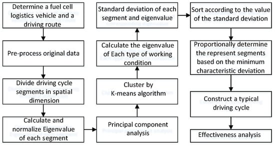
Figure 1.
Construction method of driving cycle for fuel cell logistics vehicle.
2. Data Acquisition and Preprocessing
2.1. Introduction of the DAQ Paltform
In order to monitor the operation of fuel cell vehicles and fuel cell systems in real time, and optimize energy management strategy and control systems in a timely and effective manner, so as to protect the fuel cell system to a greater extent, a remote data monitoring platform based on the on-board system is established. In this platform, the T-BOX system sends the collected vehicle information, such as the state parameters of the motor, power battery, and fuel cell system (collected by related sensors) to the cloud server via LTE, and we can perform subsequent processing on these data in the background. The relevant information of the remote data monitoring platform we are currently using is shown in Table 1.

Table 1.
The introduction of our data acquisition platform.
2.2. Determination of Driving Route
At present, our fuel cell logistics vehicles are mainly operated in Guangdong Province and Shanghai. Considering that in the preliminary research process, we hope that the sample route we choose will cover as many road types as possible, which will help us follow-up on optimizing the energy management and the control strategy, so we chose a route of the logistics vehicle in Yunfu City, Guangdong Province for research, as shown in Figure 2. The whole path is 92 km in length and takes the fuel cell logistics vehicle for about 2 hours. This route covers various types of roads such as national highway, urban road and highway, and 42-day data is collected.
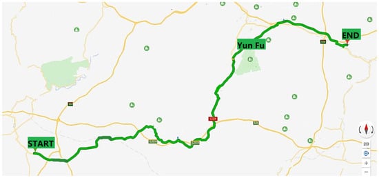
Figure 2.
The selected driving route.
After determining the sample driving route, we can acquire the route’s terrain profile by using Google Earth software, the terrain data is shown in Figure 3.
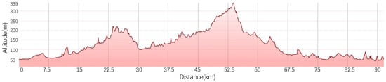
Figure 3.
The terrain of the route.
The impact of terrain on the fuel cell system is mainly reflected in the intake pressure of the air compressor, because the power level of fuel cell system we use at this stage is not very large, taking into account the cost and policy factors, if we choose a cross very high and very low altitude routes, then the controller design of the fuel cell system will have great challenges, the actual output power will be greatly reduced. As can be seen from the above figure, the maximum altitude of the sample driving route we selected is 339 m, which is less than the maximum altitude required by the real drive emission(RDE) [17] test to not exceed 700 m, but at the same time, the difference of the altitude of the whole journey in our route is about 300 m, which exceeds the requirement of an altitude difference of less than 100 m in the RDE test. Considering that our logistics vehicles usually travel between cities, this prerequisite makes us difficult to find in the existing database that the road features are rich as well as the altitude difference is small, so we choose to appropriately relax the restriction on altitude difference.
2.3. Data Preprocessing
After acquiring the original data, we need to perform data preprocessing on the original data, which mainly includes the following aspects: judgment of invalid operating data, outlier detection and data filtering.
(1) Judgment of invalid operating data
This part is mainly due to the fact that after the vehicle is started or stopped, although the data acquisition system has sent the vehicle information to the cloud during this period, in fact, the vehicle has not displaced. Therefore, we have eliminated them through human judgment.
(2) Outlier detection
This part is mainly due to the signal interruption in the data communication process, which is eliminated by the method of outlier detection in this research work.
(3) Data filting
Because the original data is noisy, it needs to be filtered. In this research, the method of moving average filter is used to filter the original data.
3. Clustering of Vehicle Working Conditions Based on K-Means
3.1. Division of Working Conditions
The time-velocity sequence is divided into many segments along the time axis as shown in Figure 4. The data are available in a Supplementary File named as “supplementary.csv”, the sampling time is 1 second and the speed is in kilometer per hour.Considering the accuracy and complexity of the calculation, every segment is 1 kilometer long and it’s assumed that the vehicles dynamic parameters in one particular segment are basically the same.
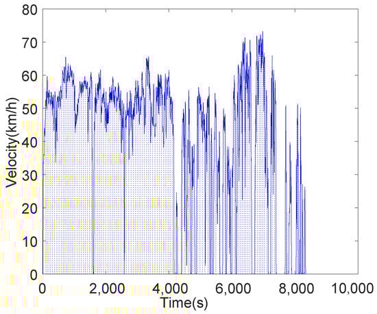
Figure 4.
The division of time-velocity sequence in a certain day.
3.2. Selection of Characteristic Parameters
This paper refers to a literature [18] when selecting the characteristic parameters, additionally the throttle pedal angle and brake pedal angle are taken into account. The characteristics are chosen as listed in Table 2 [19].
Table 2.
The list of selected characteristic parameters.
However, after a correlation analysis of the parameters all above, it’s found that the correlation coefficient of the throttle and brake pedal angle reaches nearly 1. So the throttle and brake pedal angle are eliminated from the parameters group. The calculation formulas for above parameters are as follow.
(1) Average vehicle speed
where n is the number of data points in each working condition segement, and is the vehicle speed when the i-th data point corresponds to the working condition segement.
(2) Average vehicle speed (neglecting parking situations)
(3) Standard deviation of vehicle speed
(4) Maximum acceleration is the maximum value of acceleration of each segement.
(5) Average acceleration while accelerating
where is the number of data points with positive acceleration in each segement, and is the vehicle acceleration at the -th data point in the segement.
(6) Minimum acceleration is the minimum value of acceleration of each segement.
(7) Average acceleration while decelerating
where is the number of data points with negative acceleration in each segement, and is the vehicle acceleration when the -th data point corresponds to the segement.
(8) Acceleration ratio
(9) Deceleration ratio
(10) Idling ratio
where is the number of data points where the vehicle speed is zero in each segement.
(11) Standard deviation of acceleration
where is the acceleration corresponding to the i-th data point in the segement, and is the average acceleration of the segement.
(12) Standard deviation of jerk
where is the impact degree corresponding to the i-th data point in the segement, is the average jerk of the segement.
(13) The accelerator pedal opening is obtained through the fuel cell vehicle remote monitoring platform.
(14) The brake pedal opening is obtained through the fuel cell vehicle remote monitoring platform.
In summary, a characteristic parameter vector of 12 elements is formed as follows.
3.3. Principal Component Analysis
In order to avoid over-fitting problem, it is necessary to do dimensionality reduction to the data before cluster analysis and principal component analysis (PCA) [20] is used. Since maximum acceleration and minimum acceleration do not contribute much, PCA is conducted on the rest 12 characteristic parameters.
In general, when the sum of the variance’s contribution of several principal component reaches up to 85%, these principal components are believed to be able to describe most of the information of the original data [21]. The results obtained by PCA are shown in Figure 5 and Figure 6.
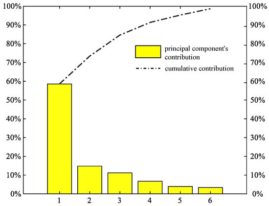
Figure 5.
The cumulative contribution of first 6 principal components.
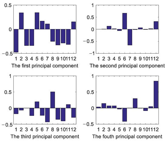
Figure 6.
The linear combination coefficients for first four principal components (The number on the x-axis coordinate corresponds to the serial number in Table 2).
In Figure 5, the cumulative contribution of the first 4 principal components reaches 90%. Figure 6 shows the linear combination coefficients of the twelve characteristics. The higher the absolute value of the combination coefficient is, the stronger is the relationship between the principal component and the characteristics [22].
3.4. Clustering of Working Conditions
This paper uses K-means algorithm to cluster all segments in the principal component domain [23]. Before K-means algorithm is conducted, a proper selection of the parameter K is essential. A theory, which is called Elbow method, uses sum of the squared errors(SSE) to find the proper K. This criteria is defined as formula below.
in which p is the point to be clustered, is the cluster center, means the Euler distance between them, k is the number of cluster center. It’s obvious that SSE decreases as K increases, however, there exists an inflection point in the curve. When K is bigger than the inflection point, little improvement of SSE is achieved. Thus, the proper selection of the parameter K is the inflection point of the SSE curve, which is shown in Figure 7.
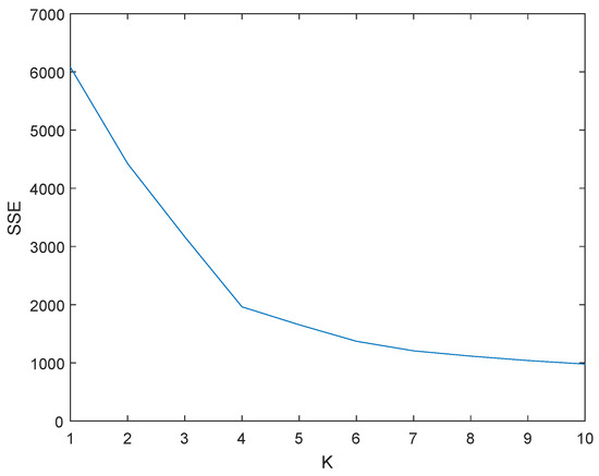
Figure 7.
Cluster parameter K versus SSE.
Then set the cluster number as 4 and do the clustering to the data above. To show the cluster result intuitively, all the segments are labeled in the three-dimension coordinate composed of three principal components, as shown in Figure 8.
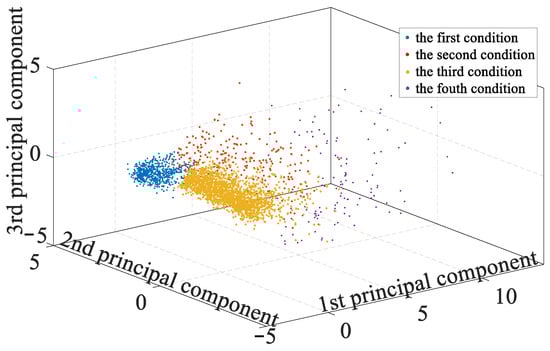
Figure 8.
The clustering result of segments.
In reference to the statistical analysis of the clustering result, the four clustered sets are defined as four different driving conditions, which is respectively highway, urban road, national highway and others. Average values of these twelve parameters for the four conditions are shown in Table 3. RDE test simply divides three driving conditions from each other with maximum speed. On the contrary, this paper take not only the maximum speed, but also the average speed, ratio of idling and deviation of the acceleration into account. In Highway presents the highest average speed and lowest average acceleration and the deviation of acceleration, indicating that the road condition is clear. Urban road presents a lowest average speed and shows relatively high ratio of idling, deviation of acceleration. Nation highway shares a relatively high average speed but lower than that of the highway, and shows a low deviation of acceleration. Others shows a lowest average speed and highest ratio of idling, which means there whether exists a traffic jam or simply a start-stop scenario.
Table 3.
Average values of characteristic parameters of four conditions.
The information of the whole journey validates the correctness of the the clustering result. The proportion of the four types of driving condition (highway: urban road: national highway: others) is 544: 856: 2498: 128. It’s clear that the proportions of the driving conditions in real route is similar to the clustering result. In comparison to the RDE test, which stipulates that the proportion of city, rural and motorway should be 34%, 33% and 33%, and the error of the proportion should be between −10% and +10%. It’s one of the great difference of the road map construction method with the fuel cell vehicle.
4. Construction of Typical Driving Cycle
In accordance to the proportion of the four types of driving conditions, 10 segments of National highway, 3 of Urban road and 4 of Highway are selected from the bank of segments. They are combined together in a certain sequence, which is the same to the order these driving conditions occur on the real route, as shown in Figure 9. Besides, 2 segments from Others driving conditions are added at the start and the end of the route.
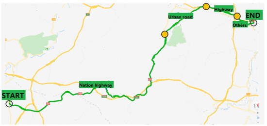
Figure 9.
The segmentation of route in map.
In order to find the most representative driving segments, a criteria, shown in Equation (13) is introduced and it may find the minimum of the deviation between a certain driving segment with its cluster center.
where is the deviation of a segment in this type of driving condition, is the eigenvalue in the principal component space of a driving segment, is the mean value of the eigenvalue in the j-th (j = 1, 2, 3, 4) type of driving condition, and is the number of eigenvalues. The calculation had been done and the best result is shown in Table 4.
Table 4.
Selected driving segments and their deviations.
The driving cycle was formed by connecting the chosen segments in order. In this case, there would possibly exist discontinuities between every two segments. In order to solve this problem, this paper uses moving filter method to smooth the driving cycle curve. Finally, the typical driving cycle of fuel cell logistics vehicle is formed as shown in Figure 10. The whole driving cycle is 18 km in length, lasting for 1581 seconds.
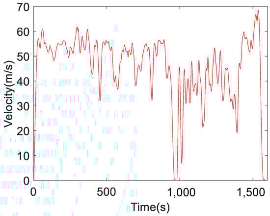
Figure 10.
Constructed driving cycle of fuel cell logistics vehicle.
5. Effectiveness Analysis of Driving Cycle
In order to validate the driving cycle, this paper calculates the errors of the characteristic parameters between the original data and the cycle built in this paper. Two equations, as shown in Equations (14) and (15), are introduced:
where is the relative error of each characteristic parameter, and is the average error derived from . A is the average value of a characteristic parameter of the original data, is that of the cycle built in this paper. The result shows the average error between the original data and the cycle is only 7.9%.
Furthermore, this paper calculates the speed acceleration () probability distribution (SAPD) of the original data and the cycle. The velocity distribution is between 0 and 75 km/h, and the acceleration distribution is between -4 and 4 . The specific result is shown in Table 5.
Table 5.
Velocity-acceleration () probability distribution matrix of the original data/cycle(%).
In this paper, the cosine similarity theorem is used to judge the similarity of the distribution probability matrix of the original data and the cycle [24]. First, the above two distribution probability matrices are converted into two vectors a and b. The equation for cosine similarity is shown in Equation (16):
where is the cosine similarity and is the angle of two vectors. The result is 0.9903, which is very close to 1, indicating that the driving cycle constructed in this paper are very similar to the original one.
6. Discussion
Nowadays, there are not many fuel cell vehicles actually running on the roads of China, resulting in not much feedback on the development of fuel cell systems based on actual driving cycle. Therefore, the purpose of this article is mainly to focus on an existing structured road with fuel cell commercial logistics vehicles running every day, as a research to promote subsequent fuel cell system development, such as energy management research, control system optimization, and so on.
This study proposed a methodology to construct a representative driving cycle of fuel cell vehicles in Guangdong Province. After being pre-processed, the original data are divided in spatial dimension. Characteristic parameters are derived and K-means algorithm for cluster analysis is used. The results of the effectiveness analysis show that the typical driving cycle we constructed can cover the original data well and reflect the four road structures of highway, urban road, national highway and others.
In the process of constructing the driving cycle, a few prominent differences between fuel cell vehicles (FCV) and internal combustion engine vehicles (ICEV) are shown. For example, a fuel cell logistics vehicle have higher average velocity and smooth acceleration due the its cruising on a highway, which suggests that the occurrence possibility of highway conditions is the most. However, a fuel cell logistics vehicle has a much lower maximum speed no more than 80 km/h, which leads to a lower energy consumption when the cycle is used for vehicle power analysis. The facts above proves again the necessity of building an independent driving cycle for FCV. The validity analysis of the driving conditions has provided an outstanding evidence of the correctness of the driving cycle built in this paper, and the cycle can be taken as basis for the optimization research of energy management strategies of fuel cell powertrain system. As more and more enterprises pay much attention on the development and application of commercial vehicles that run on a typical route, it’s possible for the researchers in those enterprises to analyze the energy consumption along the route following the procedure this paper puts forward, and plans wisely where a gas station should be built.
Supplementary Materials
The following are available online at https://www.mdpi.com/2032-6653/12/1/5/s1.
Author Contributions
Conceptualization, S.Z.; Data curation, J.J.; Formal analysis, J.J.; Methodology, J.J.; Project administration, S.Z.; Supervision, S.Z.; Writing—review & editing, Y.W. All authors have read and agreed to the published version of the manuscript.
Funding
This research received no external funding.
Institutional Review Board Statement
Not applicable. The study did not require ethical approval and not involve humans or animals.
Informed Consent Statement
Not applicable. The study did not involve humans.
Data Availability Statement
The data presented in this study are available in Supplementary File, which is named as “supplementary.csv”.
Conflicts of Interest
There is no conflict of interest.
References
- Bassam, A.M.; Phillips, A.B.; Turnock, S.R.; Wilson, P.A. An improved energy management strategy for a hybrid fuel cell/battery passenger vessel. Int. J. Hydrog. Energy 2016, 41, 22453–22464. [Google Scholar] [CrossRef]
- Wee, J.H. Applications of proton exchange membrane fuel cell systems. Renew. Sustain. Energy Rev. 2007, 11, 1720–1738. [Google Scholar] [CrossRef]
- Nistor, S.; Dave, S.; Fan, Z.; Sooriyabandara, M. Technical and economic analysis of hydrogen refuelling. Appl. Energy 2016, 167, 211–220. [Google Scholar] [CrossRef]
- Liu, J.; Wang, X.; Khattak, A. Customizing driving cycles to support vehicle purchase and use decisions: Fuel economy estimation for alternative fuel vehicle users. Transp. Res. Part C Emerg. Technol. 2016, 67, 280–298. [Google Scholar] [CrossRef]
- Lien, N.T.Y.; Dung, N.T. The determination of driving characteristics of Hanoi bus system and their impacts on the emission. Vietnam J. Sci. Technol. 2017, 55, 74. [Google Scholar] [CrossRef]
- Nandjou, F.; Poirot-Crouvezier, J.P.; Chandesris, M.; Rosini, S.; Hussey, D.S.; Jacobson, D.L.; Lamanna, J.M.; Morin, A.; Bultel, Y. A pseudo-3D model to investigate heat and water transport in large area PEM fuel cells—Part 2: Application on an automotive driving cycle. Int. J. Hydrog. Energy 2016, 41, 15573–15584. [Google Scholar] [CrossRef]
- Kang, S.; Min, K. Dynamic simulation of a fuel cell hybrid vehicle during the federal test procedure-75 driving cycle. Appl. Energy 2016, 161, 181–196. [Google Scholar] [CrossRef]
- Li, B.; Lin, R.; Yang, D.; Ma, J. Effect of driving cycle on the performance of PEM fuel cell and microstructure of membrane electrode assembly. Int. J. Hydrog. Energy 2010, 35, 2814–28192008. [Google Scholar] [CrossRef]
- Lin, R.; Li, B.; Hou, Y.P.; Ma, J.M. Investigation of dynamic driving cycle effect on performance degradation and micro-structure change of PEM fuel cell. Int. J. Hydrog. Energy 2009, 34, 2369–2376. [Google Scholar] [CrossRef]
- Ho, S.H.; Wong, Y.D.; Chang, V.W.C. Developing Singapore Driving Cycle for passenger cars to estimate fuel consumption and vehicular emissions. Atmos. Environ. 2014, 97, 353–362. [Google Scholar] [CrossRef]
- Shen, P.; Zhao, Z.; Li, J.; Zhan, X. Development of a typical driving cycle for an intra-city hybrid electric bus with a fixed route. Transp. Res. Part D Transp. Environ. 2018, 59, 346–360. [Google Scholar] [CrossRef]
- Shi, S.; Lin, N.; Zhang, Y.; Huang, C.; Liu, L.; Lu, B.; Cheng, J. Research on Markov property analysis of driving cycle. In Proceedings of the 2013 IEEE Vehicle Power and Propulsion Conference (VPPC), Beijing, China, 15–18 October 2013; pp. 1–5. [Google Scholar]
- Shi, S.; Lin, N.; Zhang, Y.; Cheng, J.; Huang, C.; Liu, L.; Lu, B. Research on Markov property analysis of driving cycles and its application. Transp. Res. Part D Transp. Environ. 2016, 47, 171–181. [Google Scholar] [CrossRef]
- Gao, J.D.; Qin, K.J.; Liang, R.L.; Li, M.L. Comparative analysis of medinm-duty diesel engine emissions under BJCBC and ETC. J. Jilin Univ. Technol. Ed. 2012, 42, 33–38. [Google Scholar]
- Mock, P.; Kühlwein, J.; Tietge, U.; Franco, V.; Bandivadekar, A.; German, J. The WLTP: How a new test procedure for cars will affect fuel consumption values in the EU. Int. Counc. Clean Transp. 2014, 9, 35–47. [Google Scholar]
- Yang, Z.; Wang, B.; Jiao, K. Life cycle assessment of fuel cell, electric and internal combustion engine vehicles under different fuel scenarios and driving mileages in China. Energy 2020, 198, 117365.1–117365.9. [Google Scholar] [CrossRef]
- Merkisz, J.; Jacyna, M.; Merkisz-Guranowska, A.; Pielecha, J. The Parameters of Passenger Cars Engine in Terms of Real Drive Emission Test. Arch. Transp. 2014, 32, 43–50. [Google Scholar] [CrossRef][Green Version]
- Donateo, T.; Pacella, D.; Laforgia, D. Development of an Energy Management Strategy for Plug-In Series Hybrid Electric Vehicle Based on the Prediction of the Future Driving Cycles by ICT Technologies and Optimized Maps. In Proceedings of the SAE 2011 World Congress & Exhibition, Detroit, MI, USA, 12–14 April 2011. Paper No. SAE 2011-01-0892. [Google Scholar]
- Si, L.; Hirz, M.; Brunner, H. Big Data-Based Driving Pattern Clustering and Evaluation in Combination with Driving Circumstances. In Proceedings of the SAE World Congress 2018, Detroit, MI, USA, 10–12 April 2018. Paper No. SAE 2018-01-1087. [Google Scholar]
- Abdi, H.; Williams, L.J. Principal component analysis. Wiley Interdiscip. Rev. Comput. Stat. 2010, 2, 433–459. [Google Scholar] [CrossRef]
- Xie, H.; Tian, G.; Chen, H.; Wang, J.; Huang, Y. A distribution density-based methodology for driving data cluster analysis: A case study for an extended-range electric city bus. Pattern Recognit. 2018, 73, 131–143. [Google Scholar] [CrossRef]
- Berzi, L.; Delogu, M.; Pierini, M. Development of driving cycles for electric vehicles in the context of the city of Florence. Transp. Res. Part D Transp. Environ. 2016, 47, 299–322. [Google Scholar] [CrossRef]
- Wang, Q.; Huo, H.; He, K.; Yao, Z.; Zhang, Q. Characterization of vehicle driving patterns and development of driving cycles in Chinese cities. Transp. Res. Part D Transp. Environ. 2008, 13, 289–297. [Google Scholar] [CrossRef]
- Allaire, G.; Kaber, S.M. Numerical Linear Algebra; Springer: Berlin/Heidelberg, Germany, 2008; Volume 55. [Google Scholar]


Publisher’s Note: MDPI stays neutral with regard to jurisdictional claims in published maps and institutional affiliations. |
© 2021 by the authors. Licensee MDPI, Basel, Switzerland. This article is an open access article distributed under the terms and conditions of the Creative Commons Attribution (CC BY) license (http://creativecommons.org/licenses/by/4.0/).