Eco-Driving for Different Electric Powertrain Topologies Considering Motor Efficiency

Abstract

Electrification and automatization may change the environmental impact of vehicles. Current eco-driving approaches for electric vehicles fit the electric power of the motor by quadratic functions and are limited to powertrains with one motor and single-speed transmission or use computationally expensive algorithms. This paper proposes an online nonlinear algorithm, which handles the non-convex power demand of electric motors. Therefore, this algorithm allows the simultaneous optimization of speed profile and powertrain operation for electric vehicles with multiple motors and multiple gears. We compare different powertrain topologies in a free-flow scenario and a car-following scenario. Dynamic Programming validates the proposed algorithm. Optimal speed profiles alter for different powertrain topologies. Powertrains with multiple gears and motors require less energy during eco-driving. Furthermore, the powertrain-dependent correlations between jerk restriction and energy consumption are shown.

1. Introduction

In the European Union in 2018, only 0.05% of the final energy consumption of road-based mobility is electricity [1]. However, today’s mega trends such as urbanization and sustainability require a shift in road-based mobility systems toward more efficient and environmentally friendly transport. The advent of Connected Autonomous Vehicles (CAVs) may change the environmental impact of mobility. Kopelias et al. [2] give a literature review of possible factors affecting the environmental impact of CAVs and refer to the vehicle, network and user. The vehicle itself may be affected by alternative fuels or electric powertrains, new vehicle size and design as well as intelligent operation such as energy-efficient driving, platooning and intelligent route choice.

Vehicle design, powertrain and operation may change for a CAV. Anselma and Belingardi [3], Tate et al. [4] and Gambhira [5] incorporate energy-efficient driving in powertrain optimization process to gain a CAV-optimized powertrain. However, in comparison to state-of-the-art powertrain optimizations for human-driven electric vehicles [6,7], the design space is narrow. Anselma and Belingardi [3] only review a single electric motor with a single-speed transmission. Gambhira [5] examines a second powered axle. However, electric powertrains may consist of multiple motors and gears as a second driven axle and/or a second gear may result in efficiency gains [8], ([9] p. 86ff). Furthermore, the implemented energy-efficient driving scenarios are simplified and therefore are not realistic. Anselma and Belingardi [3] and Gambhira [5] use Dynamic Programming (DP) to calculate speed profiles. Since DP is computationally expensive, the speed profiles are generated offline for fixed boundary conditions. Thus, leading vehicles can not be simulated realistically. Tate et al. [4] optimize the speed profile by smoothing a driving cycle.

Sciarretta [10] gives a summary about energy-efficient driving: minimal-energy route navigation, anticipating the road, signal phase and timing, energy-efficient car-following and others may reduce energy demand of vehicles. However, the potential savings in literature differ greatly. For anticipated car-following, Sciarretta ([10] p. 14f) reviewed literature that shows efficiency gains ranging from 0–44% with respect to the leading vehicle. This range can be explained by different boundary conditions and methodologies.

Energy-efficient driving methodologies may be divided into online and offline applications. DP is often used as an offline method ([10] p. 164), [11,12,13], since it can compute the global optimal solution using nonlinear functions and efficiency maps present as look-up tables (LUT). Online applications may be used in a model predictive control (MPC) and react to changing boundary conditions, such as leading vehicles. For fast computation, these models are often simplified.

Furthermore, methodologies can be incorporated in the three main areas:

• “wheel-to-distance” optimization
• “tank-to-distance” optimization
• minimization of $a^2$

Han et al. [14] describe “wheel-to-distance” and “tank-to-distance” optimizations. The former neglects the vehicle’s powertrain efficiency, minimizing the power at the wheel. The latter incorporates the efficiency of the powertrain. Another widely used technique is the minimization of squared acceleration, especially in car-following scenarios, due to the quadratic formulation of the problem and thereby fast optimization methods [15,16,17].

According to Han et al. [14], an optimal “wheel-to-distance” speed profile consists of three to four stages. If no traffic is regarded, the vehicle should accelerate/decelerate as fast as possible to a specific speed, keep that speed constant and decelerate with coasting and/or maximal braking, depending on the vehicle’s recuperative ability.

The powertrain’s efficiency is examined for “tank-to-distance”. Thus, the optimal speed profile depends on the chosen powertrain. Han et al. [14] differentiate between a combustion and an electric powertrain. Due to the combustion engine’s poor efficiency at low load, cruising may not as efficient as a periodic alternation between acceleration and coasting. This results in what is referred to as a pulse-and-glide (P&G) strategy. Eo et al. [18] proof savings through P&G on a dynamo-meter for a parallel hybrid electric vehicle (HEV). Li and Peng [19] optimize the speed profile for a gasoline engine with a continuously variable transmission (CVT), assuming optimal control and constant efficiency of the CVT. Thus, the optimal engine speed for each load can be calculated by curve fitting. Finally, the brake-specific fuel consumption map, which depends on engine torque and engine speed, can be reduced to a static fuel rate, depending solely on the motor power, thus reducing the computational burden. However, energy-efficient driving taking the powertrain’s efficiency into consideration may have multiple degrees of freedom, since speed and powertrain operation can be optimized. Shao ([20] p. 26ff) optimizes the speed for a combustion engine with six gears, using mixed-integer programming.

For an HEV, Guo et al. [21] decouple the problem by first minimizing the “wheel-to-distance” losses and second by optimizing powertrain operation. Other works simultaneously optimize speed profile and powertrain operation [20,22,23]. Shao [20] pre-calculates the most efficient operating points offline and saves them in linearized form. Li et al. [23] use a constant average efficiency for the electric motor and combustion engine.

For full-electric vehicles, Li et al. [24] optimize the speed profile for a four-wheel-drive electric vehicle with a motor at each wheel. However, the motor efficiency is neglected. Shao ([20] p. 93f) considers an electric vehicle with a single motor and single-speed transmission. The resulting electrical motor power depends on motor torque and speed and is approximated by a polynomial function:

$$P_{\mathrm{el}}=c_{00}+c_{10}{\omega }_{\mathrm{m}}+c_{01}{T}_{\mathrm{m}}+c_{11}{\omega }_{\mathrm{m}}{T}_{\mathrm{m}},$$

(1)

where $c_{00}$, $c_{10}$, $c_{01}$ and $c_{11}$ are fitting coefficients and ${\omega }_{\mathrm{m}}$ and $T_{\mathrm{m}}$ the motor speed and motor torque, respectively. Lelouvier et al. [25] optimize the energy consumption of a platoon of electric vehicles with an MPC. The electric power of the electric motor is modeled based on Reference [26] with the polynomial function:

$$P_{\mathrm{el}}=c_1{\omega }_{\mathrm{m}}{T}_{\mathrm{m}}+c_2{T}_{\mathrm{m}}^2,$$

(2)

with the fitting coefficients $c_1$ and $c_2$. Han et al. [14] neglect battery losses and aerodynamic drag and approximate the electric motor power, which is also based on Equation (2), with $c_1=1$. This results in a parabolic speed profile for the electric vehicle. Padilla et al. [27] optimize the speed profile using sequential quadratic programming by minimizing the consumed power, representing an electric motor by a quadratic function. All regarded electric vehicles considering motor efficiency consist of a powertrain with one motor and single-speed transmission.

Minimizing acceleration avoids unnecessary accelerations and thus saves energy. Dollar and Vahidi [15] optimize the speed for a platoon, of which the leading vehicle drives different driving cycles. Efficiency gains are higher for more transient speed profiles of the leading vehicle, showing the impact of the chosen boundary conditions. Wegener et al. [17] determine the eco-driving potential of different powertrains by optimizing the speed by minimizing acceleration. The gained speed profile is used to calculate the energy consumption of the different powertrains. However, this approach determines how well the powertrains fit to the resulting speed profile and do not exploit the full potential of the various powertrains.

In powertrain simulation, energy consumption is often gained by LUTs representing motor efficiency ([28] p. 87). The required electrical power, gained by motor efficiency maps, is non-convex, since efficiency drops for low torques and speeds (Figure A1 in Appendix A). So et al. [12] use DP with an efficiency map of an electric motor for an electric powertrain with one motor and a single-speed transmission and showed that energy-efficient driving of an electric powertrain may result in P&G. Except works that use DP, all further reviewed studies approximate the power of the electric motor by quadratic functions of torque and speed or minimize acceleration. If acceleration is minimized, the energy demand must be calculated retrospectively. Thus, the energy savings are due to avoiding unnecessary acceleration and braking but not due to efficiently using the powertrain. Quadratic representations of energy demand do not represent the motor efficiency for low torques. Thus, these techniques result in non-optimal speed profiles. Furthermore, electric powertrains may consist of multiple motors and gears as a second driven axle or a second gear may result in efficiency gains. By adding multiple gears or powered axles, powertrain operation and speed profile may be simultaneously optimized.

To the authors’ knowledge, there exist no online capable eco-driving algorithm that take realistic motor efficiency into account. In addition, no work was found that considers multiple motors and multiple gears while simultaneously considering motor efficiency. Therefore, the scope of the paper is:

• To formulate an online capable optimization of vehicle speed and powertrain operation for different electric powertrain topologies, taking realistic motor efficiency into account.
• To compare the optimization to a quadratic representation of the electrical power and to the minimization of acceleration, which are widely used in literature.
• To verify the optimization by a DP algorithm.

2. Methods

In this section we introduce the new eco-driving nonlinear programming (NLP) algorithm, which allows a simultaneous optimization of speed profile and powertrain operation for different electric powertrain topologies, taking realistic motor efficiency into account. Next, the DP algorithm, which is used to verify the results, is introduced. Finally, the case studies are presented, which are used to determine the eco-driving potential for different powertrain topologies.

2.1. Eco-Driving-Algorithm

To gain energy efficient speed profiles for different powertrain topologies, an optimal control problem (OCP) is transcibed into a NLP with the cost function J, the states $x$, the control input $u$ and the equality constraints $h_i$ and inequality constraints $g_j$:

$$\begin{array}{cc}\underset{x,u}{\min }\hfill & J(x,u)\hfill \\ \mathrm{s}.\mathrm{t}.\hfill & \frac{\mathrm{d}x}{\mathrm{d}t}=f(x(t),u(t))\hfill \\ & h_i=0\hfill \\ & g_j\le 0\hfill \end{array}$$

(3)

The state vector consists of acceleration a, velocity v and distance s:

$$x={\left[\begin{array}{ccc}a& v& s\end{array}\right]}^{\mathsf{T}}.$$

(4)

The size of the control vector depends on the powertrain topology. For each motor k and each transmission gear r, a traction torque $T_{\mathrm{T}}^{kr}$ and braking torque $T_{\mathrm{B}}^{kr}$ is added, where $T_{\mathrm{B}}$ describes the braking torque due to recuperation of the motor. A friction brake is not examined, as this is not used for an electric vehicle during eco-driving. The distinction between traction torque $T_{\mathrm{T}}$ and braking torque $T_{\mathrm{B}}$ allows an efficient description of the discontinuity of the transmission’s and motor’s efficiency around zero torque. Thus, Equation (5) represents a topology with two motors, of which the first one has a two-speed transmission:

$$u={\left[\begin{array}{cccccc}{T}_{\mathrm{T}}^{11}& T_{\mathrm{B}}^{11}& T_{\mathrm{T}}^{12}& T_{\mathrm{B}}^{12}& T_{\mathrm{T}}^{21}& T_{\mathrm{B}}^{21}\end{array}\right]}^{\mathsf{T}}.$$

(5)

To avoid a simultaneous use of one motor’s traction and recuperation torque or the simultaneous use of two gears, complementarity constraints are introduced, which will be explained later. The state transitions are incorporated in the equality constraints and can be formulated as:

$$\dot{a}=\frac{\mathrm{d}a}{\mathrm{d}t}$$

(6)

$$\dot{v}=\frac{1}{m\lambda }\left(-F_{\mathrm{roll}}-F_{\mathrm{air}}-F_{\mathrm{slope}}+F_{\mathrm{pt}}\right)$$

(7)

$$\dot{s}=v,$$

(8)

with the vehicle mass m, the rotational inertia factor $\lambda$, which represents an additional mass due to the spin of rotating mass ([29] p. 82), the roll resistance force $F_{\mathrm{roll}}$, the air resistance force $F_{\mathrm{air}}$, the slope resistance force $F_{\mathrm{slope}}$ and the powertrain force $F_{\mathrm{pt}}$, where

$$F_{\mathrm{roll}}=mg{f}_{\mathrm{r}}cos\left(\alpha \right)$$

(9)

$$F_{\mathrm{air}}=0.5{\rho }_{\mathrm{a}}{c}_{\mathrm{a}}{A}_{\mathrm{a}}{v}^2$$

(10)

$$F_{\mathrm{slope}}=mgsin\left(\alpha \right)$$

(11)

$$F_{\mathrm{pt}}=\sum _{k=1}^K\sum _{r=1}^{R^k}\frac{i_{\mathrm{gb}}^{kr}}{r_{\mathrm{w}}}\left({\eta }_{\mathrm{gb}}^{kr}{T}_{\mathrm{T}}^{kr}+\frac{1}{{\eta }_{\mathrm{gb}}^{kr}}{T}_{\mathrm{B}}^{kr}\right),$$

(12)

with the gravity g, the roll resistance constant $f_{\mathrm{r}}$, the slope $\alpha$, the air density ${\rho }_{\mathrm{a}}$, the air resistance constant $c_{\mathrm{a}}$, the vehicle front surface $A_{\mathrm{a}}$, the number of motors K, the number of gears for the $k\mathrm{th}$ motor $R^k$, the wheel radius $r_{\mathrm{w}}$, the constant gearbox efficiency ${\eta }_{\mathrm{gb}}^{kr}$ and gear ratio $i_{\mathrm{gr}}^{kr}$ for motor k and gear r, respectively.

Furthermore, the OCP is restricted by inequality constraints $g_j$, with the maximal traction power $P_{\max }^k$, maximal recuperation power $P_{\min }^k$, maximal traction torque $T_{\max }^k$ and maximal recuperation torque $T_{\min }^k$ for each motor k. Here, the inequality constraints are represented as box constraints:

$$j_{\min }\le \frac{\mathrm{d}a}{\mathrm{d}t}\le j_{\max }$$

(13)

$$a_{\min }\le a\le a_{\max }$$

(14)

$$v_{\min }\le v\le v_{\max }$$

(15)

$$s_{\min }\le s\le s_{\max }$$

(16)

$$P_{\min }^k\le \frac{T_{\mathrm{T}}^{kr}v{i}_{\mathrm{gb}}^{kr}}{r_{\mathrm{w}}}\le P_{\max }^k$$

(17)

$$0\le T_{\mathrm{T}}^{kr}\le T_{\max }^k$$

(18)

$$T_{\min }^k\le T_{\mathrm{B}}^{kr}\le 0.$$

(19)

The required electrical power $P_{\mathrm{el}}$ of each motor is determined by two sixth-degree bivariate polynomial functions $P_{\mathrm{el},\mathrm{T}}$ and $P_{\mathrm{el},\mathrm{B}}$ for traction and recuperation, respectively:

$$P_{\mathrm{el}}=P_{\mathrm{el},\mathrm{T}}(T_{\mathrm{T}},\omega )+P_{\mathrm{el},\mathrm{B}}(T_{\mathrm{B}},\omega ),$$

(20)

where $\omega$ represents the motor speed. The polynomial coefficients are fitted to the electrical power determined by the original motor map $P_{\mathrm{el},\mathrm{LUT}}$ by minimizing the quadratic difference between the fit and original motor map at $N_{\mathrm{LUT}}$ operating points. To gain realistic behavior, boundary conditions are introduced, forcing the electrical power to be zero for $T=0$ and $\omega =0$. Furthermore, an inequality constraint forcing the electrical power to be positive for $T>0$ and negative for $T<0$,

$$\begin{array}{cc}\min \hfill & {\displaystyle {\displaystyle \sum }_{j=1}^{N_{\mathrm{LUT},\mathrm{T}}}}{\left(P_{\mathrm{el},\mathrm{T}}\left(T_{\mathrm{T},j},{\omega }_j\right)-P_{\mathrm{el},\mathrm{LUT},\mathrm{T},j}\right)}^2\hfill \\ \mathrm{s}.\mathrm{t}.\hfill & P_{\mathrm{el},\mathrm{T}}\left(T_{\mathrm{T}}=0,\omega \right)=0\hfill \\ & P_{\mathrm{el},\mathrm{T}}\left(T_{\mathrm{T}},\omega =0\right)=0\hfill \\ & P_{\mathrm{el},\mathrm{T}}(T_{\mathrm{T}}>0,\omega )\ge 0\hfill \end{array}$$

(21)

$$\begin{array}{cc}\min \hfill & {\displaystyle {\displaystyle \sum }_{j=1}^{N_{\mathrm{LUT},\mathrm{B}}}}{\left(P_{\mathrm{el},\mathrm{B}}\left(T_{\mathrm{B},j},{\omega }_j\right)-P_{\mathrm{el},\mathrm{LUT},\mathrm{B},j}\right)}^2\hfill \\ \mathrm{s}.\mathrm{t}.\hfill & P_{\mathrm{el},\mathrm{B}}\left(T_{\mathrm{B}}=0,\omega \right)=0\hfill \\ & P_{\mathrm{e}1,\mathrm{B}}\left(T_{\mathrm{B}},\omega =0\right)=0\hfill \\ & P_{\mathrm{el},\mathrm{B}}(T_{\mathrm{B}}<0,\omega )\le 0\hfill \end{array}$$

(22)

The overall required electrical power is calculated by summing up all electrical motors K for all gears R with ${\omega }^{kr}$ representing the motor speed of motor k for gear r:

$${\omega }^{kr}=\frac{v{i}_{\mathrm{gr}}^{kr}}{r_{\mathrm{w}}}$$

(23)

$$P_{\mathrm{el},\mathrm{all}}=\sum _{k=1}^K\sum _{r=1}^{R^k}{P}_{\mathrm{el}}^k\left(T_{\mathrm{T}}^{kr},T_{\mathrm{B}}^{kr},{\omega }^{kr}\right).$$

(24)

The final cost function consists of multiple weighted sums [30]. The first two penalize jerk and acceleration, the third penalizes energy consumption of all electric motors, the fourth is used as regularization term of the control vector and the last ones are required for a realistic powertrain operation. The first of the later terms inhibits the simultaneous use of one motor’s traction and recuperation torque, the second the simultaneous use of two gears. To speed up the solver, these complementarity constraints are implemented in the cost function, similar to a soft constraint:

$$\begin{array}{c}\hfill J=\underset{\mathrm{Jerk}}{\underbrace{w_{\mathrm{j}}\int \phantom{\left({\left(\frac{d{T}_{\mathrm{T}}^{kr}}{dt}\right)}^2\right)}{\left(\frac{\mathrm{d}a}{\mathrm{d}t}\right)}^2\mathrm{d}t}}+\underset{\mathrm{Acceleration}}{\underbrace{w_{\mathrm{a}}\int \phantom{\left({\left(\frac{d{T}_T^{kr}}{dt}\right)}^2\right)}{a}^2\mathrm{d}t}}+\underset{\mathrm{Energy}}{\underbrace{w_{\mathrm{E}}\int \phantom{\left({\left(\frac{d{T}_T^{kr}}{dt}\right)}^2\right)}{P}_{\mathrm{el},\mathrm{all}}\mathrm{d}t}}+\underset{\mathrm{Regularization}}{\underbrace{\phantom{\left({\left(\frac{d{T}_T^{kr}}{dt}\right)}^2\right)}{w}_{\mathrm{r}}\int \sum _{k=1}^K\sum _{r=1}^{R^k}\left({\left(\frac{\mathrm{d}{T}_{\mathrm{T}}^{kr}}{\mathrm{d}t}\right)}^2+{\left(\frac{\mathrm{d}{T}_{\mathrm{B}}^{kr}}{\mathrm{d}t}\right)}^2\right)\mathrm{d}t}}+\\ \hfill +\underset{\mathrm{Motor}\mathrm{operation}}{\underbrace{\phantom{\left({\left(\frac{d{T}_T^{kr}}{dt}\right)}^2\right)}{w}_{\mathrm{scm}}\int \sum _{k=1}^K\sum _{r=1}^{R^k}{\left(T_{\mathrm{T}}^{kr}{T}_{\mathrm{B}}^{kr}\right)}^2\mathrm{d}t}}+\\ \hfill +w_{\mathrm{scg}}\int \sum _{k=1}^K\sum _{r=1}^{R^k-1}\\ \hfill \underset{\mathrm{Gear}\mathrm{selection}}{\underbrace{\left({\left(T_{\mathrm{T}}^{kr}\sum _{q=r+1}^{R^k}{T}_{\mathrm{T}}^{kq}\right)}^2+{\left(T_{\mathrm{T}}^{kr}\sum _{q=r+1}^{R^k}{T}_{\mathrm{B}}^{kq}\right)}^2+{\left(T_{\mathrm{B}}^{kr}\sum _{q=r+1}^{R^k}{T}_{\mathrm{B}}^{kq}\right)}^2+{\left(T_{\mathrm{B}}^{kr}\sum _{q=r+1}^{R^k}{T}_{\mathrm{T}}^{kq}\right)}^2\right)\mathrm{d}t.}}\end{array}$$

(25)

A multi-speed transmission represents a mixed integer problem. The result is highly dependent on the first guess. An initial guess is produced by a relaxed formulation of the problem—the problem is solved for a vehicle with multiple motors with different single-speed transmissions, of which each motor and transmission combination represents one gear in the multi-speed transmission. It is assumed that the lower gear ratios are more efficient. Thus, for the first guess of the actual problem, the lower gear ratio is active except for the duration where the solution of the relaxed problem had to switch on the motor with the higher gear ratio. In a second step, the NLP-solver is initialized with this guess.

2.2. Algorithm in Car-Following

For car-following, the presented algorithm is used within an MPC and is therefore adjusted. A smooth ride over a wide speed range is achieved through scaling the coefficients $w_{\mathrm{j}}$ and $w_{\mathrm{a}}$ with the square of the initial velocity $v_{\mathrm{init}}$ of the current prediction horizon:

$$w_{\mathrm{j},\mathrm{mpc}}=w_{\mathrm{j}}\times \max \left(1,v_{\mathrm{init}}^2\right)$$

(26)

$$w_{\mathrm{a},\mathrm{mpc}}=w_{\mathrm{a}}\times \max \left(1,v_{\mathrm{init}}^2\right).$$

(27)

Furthermore, the cost function is extended by two terms, the first penalizes an deviation to a nominal inter-vehicle distance, the second avoids maximum recuperation at the end of the prediction horizon by reducing the costs G by the kinetic energy scaled with $w_{\mathrm{vEnd}}$:

$$\begin{array}{c}\hfill G=J(w_{\mathrm{j}}=w_{\mathrm{j},\mathrm{mpc}},w_{\mathrm{a}}=w_{\mathrm{a},\mathrm{mpc}})+\underset{\mathrm{Inter}\text{-}\mathrm{vehicle}\mathrm{distance}}{\underbrace{\phantom{w_{\mathrm{s}}\int {\left(\Delta s-s_{\mathrm{v}0}-v{t}_{\mathrm{dn}}\right)}^2\mathrm{d}t}{w}_{\mathrm{s}}\int {\left(\Delta s-s_{\mathrm{v}0}-v{t}_{\mathrm{ref}}\right)}^2\mathrm{d}t}}-\underset{\mathrm{Kinetic}\mathrm{energy}}{\underbrace{\phantom{w_{\mathrm{s}}\int {\left(\Delta s-s_{\mathrm{v}0}-v{t}_{\mathrm{ref}}\right)}^2\mathrm{d}t}{w}_{\mathrm{vEnd}}0.5\lambda m{v}_{\mathrm{end}}^2,}}\end{array}$$

(28)

with the end velocity $v_{\mathrm{end}}$, the inter-vehicle distance $\Delta s$, a constant describing the maximal inter-vehicle distance at stand still $s_{\mathrm{v}0}$ and the reference time gap $t_{\mathrm{ref}}$. The minimum and maximum allowed distance $s_{\min }$ and $s_{\max }$ of Equation (16) are defined as:

$$s_{\min }=s_{\mathrm{lv}}+t_{\mathrm{g},\min }v$$

(29)

$$s_{\max }=s_{\mathrm{lv}}+t_{\mathrm{g},\max }v+s_{\mathrm{v}0},$$

(30)

with $s_{\mathrm{lv}}$ representing the location of the leading vehicle, $t_{\mathrm{g},\min }$ the minimal and $t_{\mathrm{g},\max }$ the maximal time gap between the vehicles.

The problem is implemented in Matlab, using CasADi [31] modeling language and the IPOPT -solver [32].

2.3. Dynamic Programming

A DP solver was implemented to verify the NLP solver results. Equation (31) presents the optimization problem, where the subscript $n$ represents the discrete time stepts from the starting point, N the number of discrete time steps, $x$ the states presented in Equation (4) and $u$ the discrete control vector, describing the actual acceleration a:

$$\begin{array}{ll}\underset{x,u}{\min }\hfill & {\displaystyle \sum _{n=1}^{N-1}}J\left(x_n,u_n\right)\hfill \\ \mathrm{s}.\mathrm{t}.\hfill & x_{n+1}=f_{\mathrm{DP}}\left(x_n,u_n\right)\hfill \\ & \begin{array}{cc}{x}_n& \in \left[x_{n,\min }{x}_{n,\max }\right]\\ u_n& \in \left[u_{n,\min }{u}_{n,\max }\right]\end{array}\hfill \end{array}$$

(31)

$f_{DP}(x_n,u_n)$ incorporates the same physics described in Equations (6)–(11). However, motor torque is calculated backward based on acceleration a and speed v. For DP, the original motor map present as LUT is used to calculate energy consumption. Inequality constraints (13)–(16) are also incorporated in the DP algorithm. This implementation generates a global optimal speed profile within the discretization with respect to all considered states.

2.4. Case Studies

To see the effects of eco-driving for different powertrain topologies, one free-flow scenario without any traffic and one car-following scenario are simulated. The first scenario is called city to city (C2C) and should represent a short highway segment. The free-flow scenario is used to see the universal effects of eco-driving for different powertrain topologies. However, in real life, leading vehicles may disturb the own speed planning. For the car-following scenario, the algorithm is used within an MPC. To test fuel economy for autonomous vehicles, Mersky and Samaras [33] suggest a car-following-test, in which a leading vehicle drives a driving cycle, while the AV has to follow the leading vehicle. Inspired by this approach, in this paper the leading vehicle is driving the worldwide harmonized light vehicles test procedure (WLTP). The prediction horizon is 10 s and the speed of the leading vehicle is assumed to be known for the prediction horizon. The boundary conditions for all scenarios as well as the driving style parameters can be seen in

Table 1. Scenario parameters.

Parameter	C2C	Car-Following
Initial acceleration	0 m/s2	0 m/s2
Final acceleration	0 m/s2	0 m/s2
Initial velocity	50 m/s	0 m/s
Final velocity	50 m/s	0 m/s
Final time	100 s	-
Final distance	2500 m	-
Minimal velocity	40 km/h	v${}_{\mathrm{lv}}$ − 18 km/h
Maximal velocity	120 km/h	v${}_{\mathrm{lv}}$ + 18 km/h
Min./max. jerk	±0.9 m/s3	±0.9 m/s3
Min. acceleration	−3.5 m/s2	−3.5 m/s2
Max. acceleration	2 m/s2	2 m/s2
Minimal time gap	-	1.5 s
Maximal time gap	-	3.5 s
Reference time gap	-	2.5 s
Max. distance at stand still	-	5 m

, where $v_{\mathrm{lv}}$ is the speed of the leading vehicle. The reference vehicle parameters are mostly inspired by the BMW i3. In addition, to see the effects of different powertrains, the vehicle’s powertrain may be extended by a second gear or a second motor at the second axle.

Table 2. Vehicle parameters.

Parameter	Value	Unit	Source
m	1320	kg	[35]
$\lambda$	1.05	-	Estimated
r	0.35	m	[35]
$A_{\mathrm{a}}$	2.8	m2	-
$c_{\mathrm{a}}$	0.29	-	[35]
$f_{\mathrm{r}}$	0.01	-	Estimated
$P_{1,\max }$	125 (PMSM)	kW	[35]
$T_{\mathrm{T}1}=-T_{\mathrm{B}1}$	250	Nm	[35]
$i_{\mathrm{gb}11}$	9.665	-	[35]
${\eta }_{\mathrm{gb}11}$	0.95	-	Estimated
$i_{\mathrm{gb}12}$	3	-	-
${\eta }_{\mathrm{gb}12}$	0.96	-	Estimated
$m_{2.\mathrm{gear}}$	20	kg	Estimated
$P_{2,\max }$	36 (IM)	kW	-
$T_{\mathrm{T}2}=-T_{\mathrm{B}2}$	110	Nm	-
$i_{\mathrm{gb}21}$	5	-	-
${\eta }_{\mathrm{gb}21}$	0.96	-	Estimated
$m_{2.\mathrm{motor}}$	80	kg	Estimated

shows the vehicle parameters, where $m_{2.\mathrm{gear}}$ and $m_{2.\mathrm{motor}}$ represent the additional mass of the two-speed transmission and second driven axle, respectively. The efficiency maps of the motors were gained by the validated tool presented in Reference [34] (Figure A1). The first is a permanent magnet synchronous motor (PMSM) and the second is an induction motor (IM).

The results of the eco-driving NLP algorithm are compared to a quadratic representation of the electric motor power, representing the state of the art and to the minimization of $a^2$ as well as to a global optimal solution determined by DP. The presented algorithm is used for the quadratic representation of motor power. However, the fit of the electric power is exchanged by a bivariate polynomial fit over the whole operation area of order one for the motor speed and order two for the motor torque, similar to Equations (1) and (2). The boundary condition of $P(\omega ,T=0)=0$ is set. This imitates the approaches of References [14,20,26]. Hereinafter, the eco-driving NLP algorithm representing motor power with bivariate polynomials of order six is referred to Poly 6 × 6 and the quadratic representation is referred to Poly 1 × 2.

The resulting speed profiles depend on the weighting factors of Equations (25) and (28). While a comparison between the Poly 6 × 6 and Poly 1 × 2 algorithms is possible with a fixed set of weighting factors, problems arise for a comparison with an $a^2$-minimization as the former weights energy to jerk and the later weights acceleration to jerk. Thus, the comparison to the $a^2$-minimization is conducted only for the C2C scenario with an additional boundary condition. First the $a^2$-minimization is conducted with the parameter set of

Table 3. Weighting factors and constraints.

Experiment (Section)	Algorithm	${\mathit{w}}_{\mathbf{j}}$	${\mathit{w}}_{\mathbf{a}}$	${\mathit{w}}_{\mathbf{E}}$	${\mathit{w}}_{\mathbf{r}}$	${\mathit{w}}_{\mathbf{scm}}$	${\mathit{w}}_{\mathbf{scg}}$	${\mathit{w}}_{\mathbf{s}}$	${\mathit{w}}_{\mathbf{vEnd}}$	${\mathit{g}}_{\mathbf{j},\mathbf{g}}$$\mathbf{Active}?$
C2C (3.2–3.4)	$a^2$	4	1	0	0	0.1	0.2	-	-	Reference
	Poly 6 × 6/Poly 1 × 2	0	0	${10}^{-3}$	0	0.1	0.2	-	-	Yes
[l]C2C-DP Comparison (4.2)	DP	250	0	${10}^{-3}$	0	0	0	-	-	No
	Poly 6 × 6	250	0	${10}^{-3}$	0	0.1	0.2	-	-	No
Car-following (3.5)	Poly 6 × 6/Poly 1 × 2	0.15	0	${10}^{-3}$	$5\times {10}^{-4}$	0.1	0.2	$5\times {10}^{-3}$	0.1	No

. Next, the speed profile’s total summed square of jerk $\sum j_{a^2}^2$ is calculated and introduced as global inequality constraints for further optimizations. Equation (32) shows the additional inequality constraint, where $m_{\mathrm{j}}$ scales the global allowed jerk for the sensitivity analysis.

$$g_{\mathrm{j}},\mathrm{g}=\sum j^2-\frac{1}{m_{\mathrm{j}}}\sum j_{\mathrm{a}}^{2}2.$$

(32)

The inital value of $m_{\mathrm{j}}$ is one. All other weights for all simulations are listed in Table 3. For all problems, $\Delta t$ is set to 0.2 s, however, for the computationally expensive DP algorithm $\Delta t$ is set to 1 s.

3. Results

The section presents the results. First, the different fits of motor power are presented, followed by the results of the free-flow scenario. First, the different algorithms are compared and later different powertrain topologies. A sensitivity analysis regarding the penalization of jerk is conducted. Last, the results of the car-following scenario are presented. It is important to note that the presented energy consumption are all calculated by the original motor efficiency maps using the calculated torques and motor speeds of the optimizations.

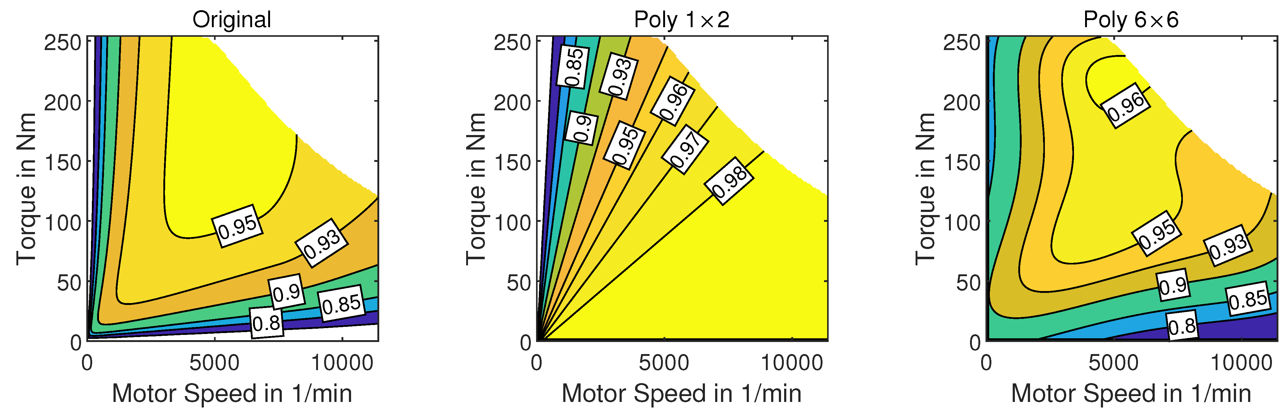
3.1. Comparison of Fits

Energy-efficient driving that minimizes the energy from “tank-to-distance” is about finding the motor’s proper operation points. Thus, to compare the fits of the electrical power, the mechanical power is divided by the electrical power to gain the motor efficiency map. This allows a good comparison of the fits. Figure 1 shows the original map, the fit of Poly 1 × 2, which represents state of the art and the new presented approach Poly 6 × 6, respectively. While Poly 6 × 6 does represent the general shape of the original motor map, the Poly 1 × 2 does not. The area of optimal efficiency of Poly 1 × 2 is at low torques, expanding for high motor speeds, whereas the original and Poly 6 × 6 have the best efficiency for high motor torque and medium speeds. As can be seen later, the imprecise fit of the Poly 1 × 2 does not allow a simultaneous optimization of vehicle speed and powertrain operation.

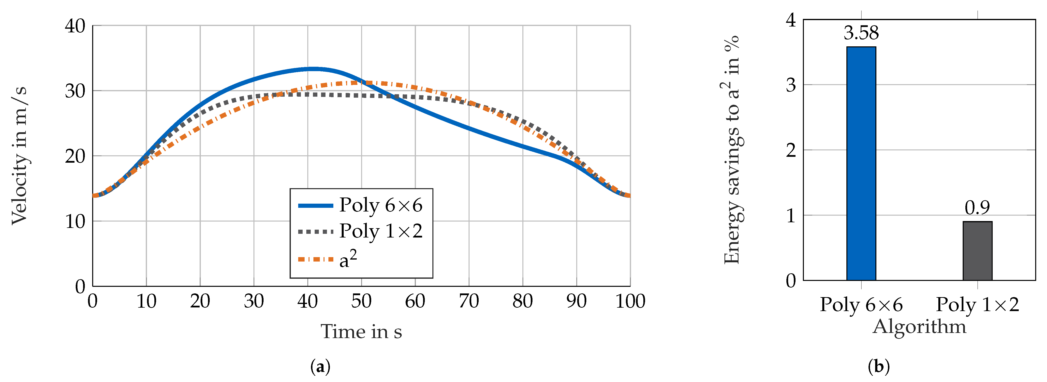
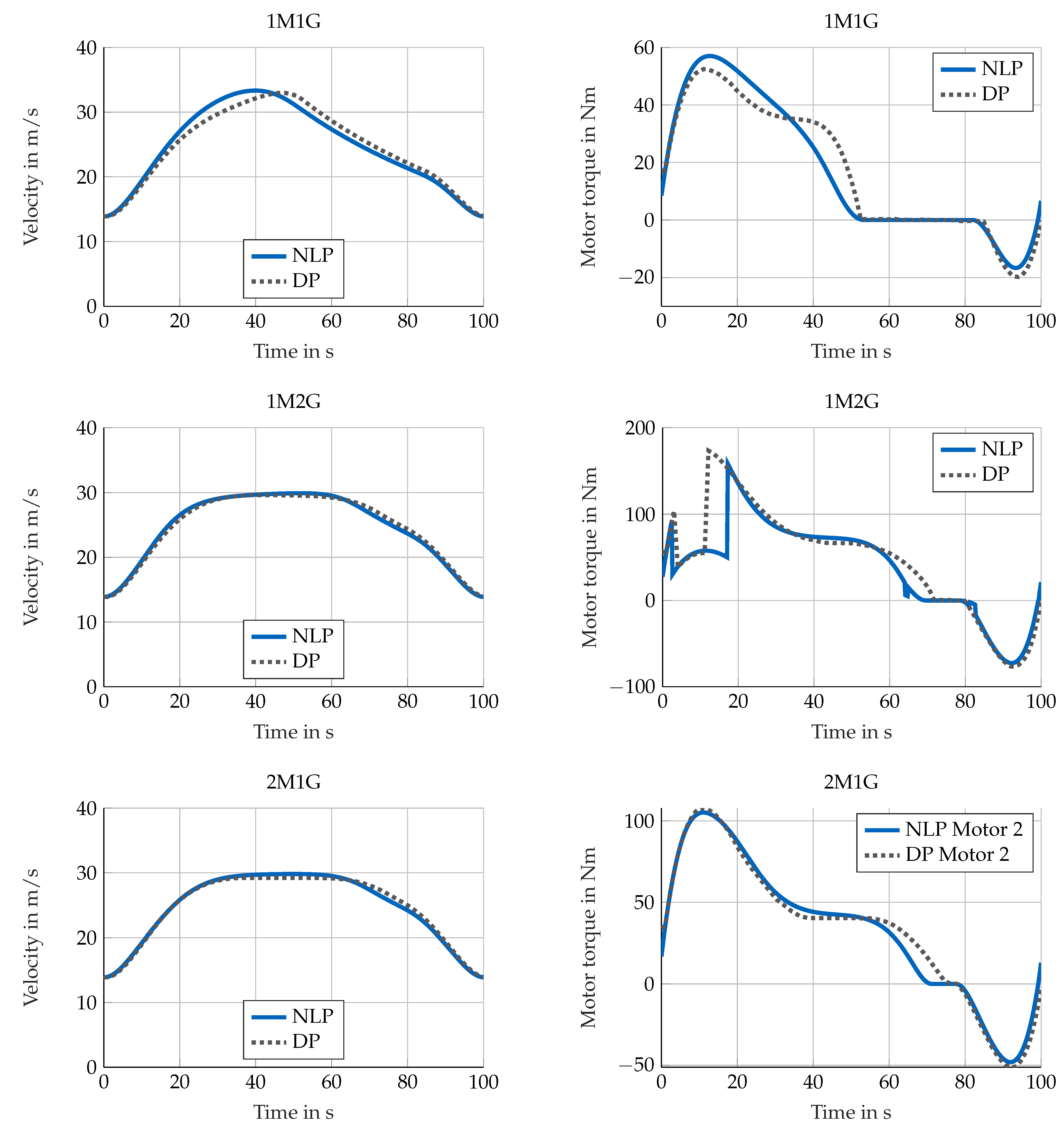
3.2. Comparison of Algorithms

The C2C scenario is used to compare the resulting speed profiles for the different algorithms. First, the powertrain consisting of one motor and single-speed-transmission is used. Figure 2a shows the resulting speed profiles for the Poly 6 × 6 algorithm, the state of art Poly 1 × 2 algorithm and the minimization of $a^2$. Figure 2b shows the energy savings compared to the $a^2$-minimization. It can be seen that the speed profiles differ. The optimization with Poly 1 × 2 accelerates, drives quasi-constant and decelerates. The Poly 6 × 6 optimization accelerates to a higher speed, coasts and decelerates (P&G). The comparison of the energy savings show an additional 2.7% of efficiency gain due to the better approximation of the electrical power with the new presented approach.

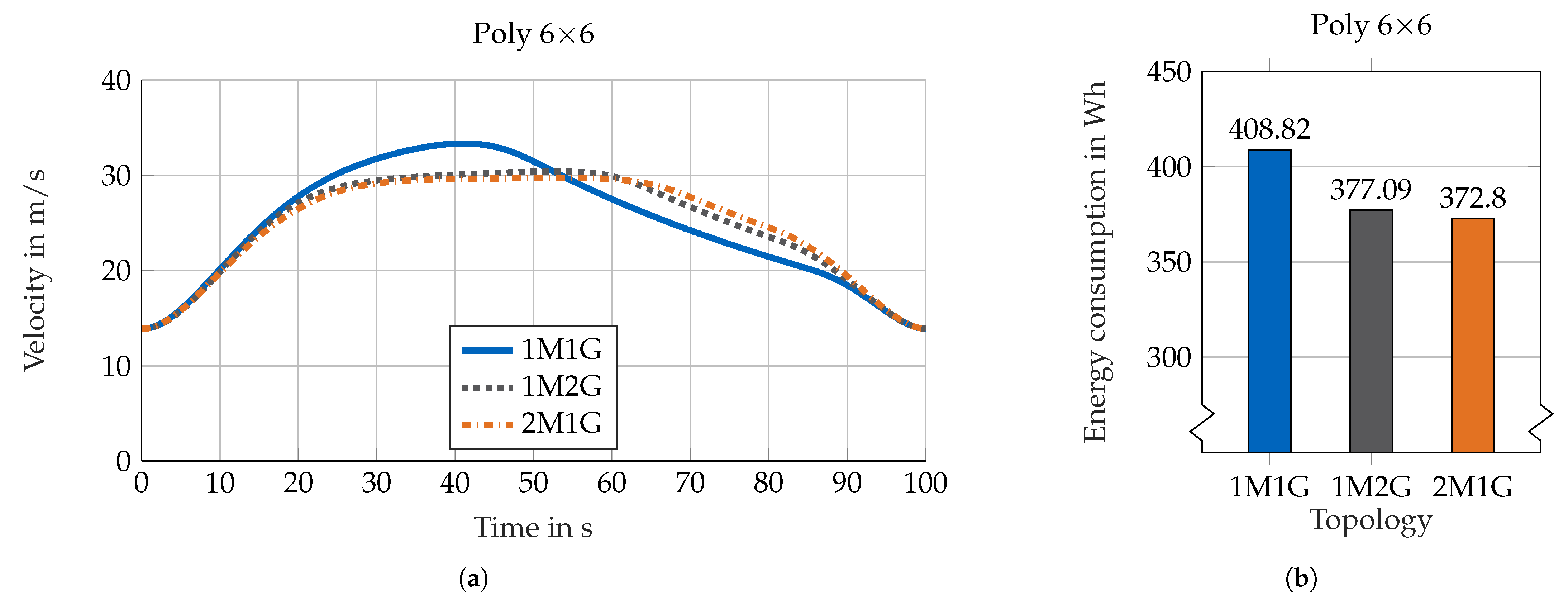
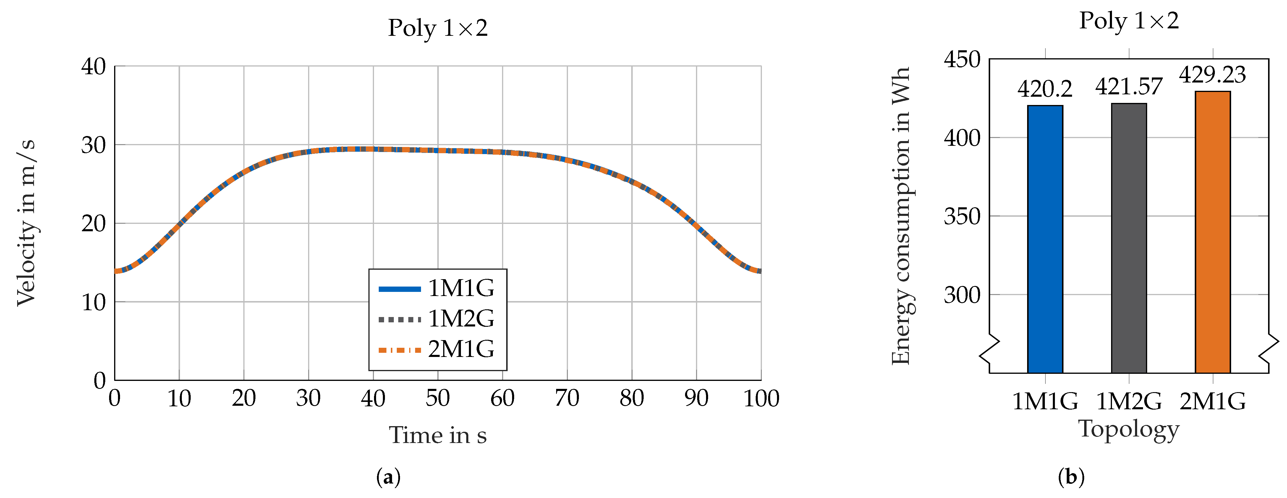
3.3. Comparison of Powertrain Topologies

Figure 3a shows the resulting speed profiles for the C2C scenarios using Poly 6 × 6 for the vehicles with one motor and single-speed-transmission (1M1G), one motor and two-speed-transmission (1M2G) and two motors with a single-speed transmission each (2M1G). All speed profiles that are based on Poly 6 × 6 consists of an acceleration, gliding and braking phase. However, the 1M2G and 2M1G topology do incorporate a phase of almost constant speed. Figure 3b shows the absolute energy consumption for the different topologies with the Poly 6 × 6 algorithm. In comparison to the 1M1G topology, 1M2G and 2M1G save 7.8% and 8.8% of energy, respectively.

Figure 4 shows the speed profiles and absolute energy consumption for the same scenario and same topologies using Poly 1 × 2. In contrast to Poly 6 × 6, the speed profiles for Poly 1 × 2 are almost identical for the different topologies. While all topologies save energy with Poly 6 × 6, the savings do not occur in the same way with Poly 1 × 2, due to a imprecise representation of the efficiency. The speed profiles do not differ since the original motor with its gear ratio is chosen as optimal operation mode most of the time. Thus, the actual energy consumption, calculated by the original motor efficiency map, rises by 0.3% for the 1M2G and 2.2% for the 2M1G in comparison to the 1M1G topology due to the increased vehicle weight.

Table 4. C2C results.

Algorithm		1M1G	1M2G	2M1G
$a^2$	Abs. in Wh	424.0	379.9	377.1
Poly 1 × 2	Abs. in Wh	420.2	421.6	429.2
	Rel. difference to $a^2$ in %	−0.9	+11	+13.8
Presented Poly 6 × 6	Abs. in Wh	408.8	377.1	372.8
	Rel. difference to $a^2$ in %	−3.6	−0.7	−1.1
	Rel. difference to Poly 1 × 2 in %	−2.8	−11.8	−15.1

summarizes the absolute energy consumption for different powertrain topologies using Poly 1 × 2 and Poly 6 × 6 and the relative difference to the $a^2$ and Poly 1 × 2 minimization of the regarded powertrain topology. To obtain the energy consumption of the $a^2$ minimization, the speed profile is calculated first and then constrained to optimize powertrain operation with the Poly 6 × 6 optimization. The results show that the 1M1G topology is able to reduce the energy consumption by the greatest extent in comparison to the $a^2$ minimization.

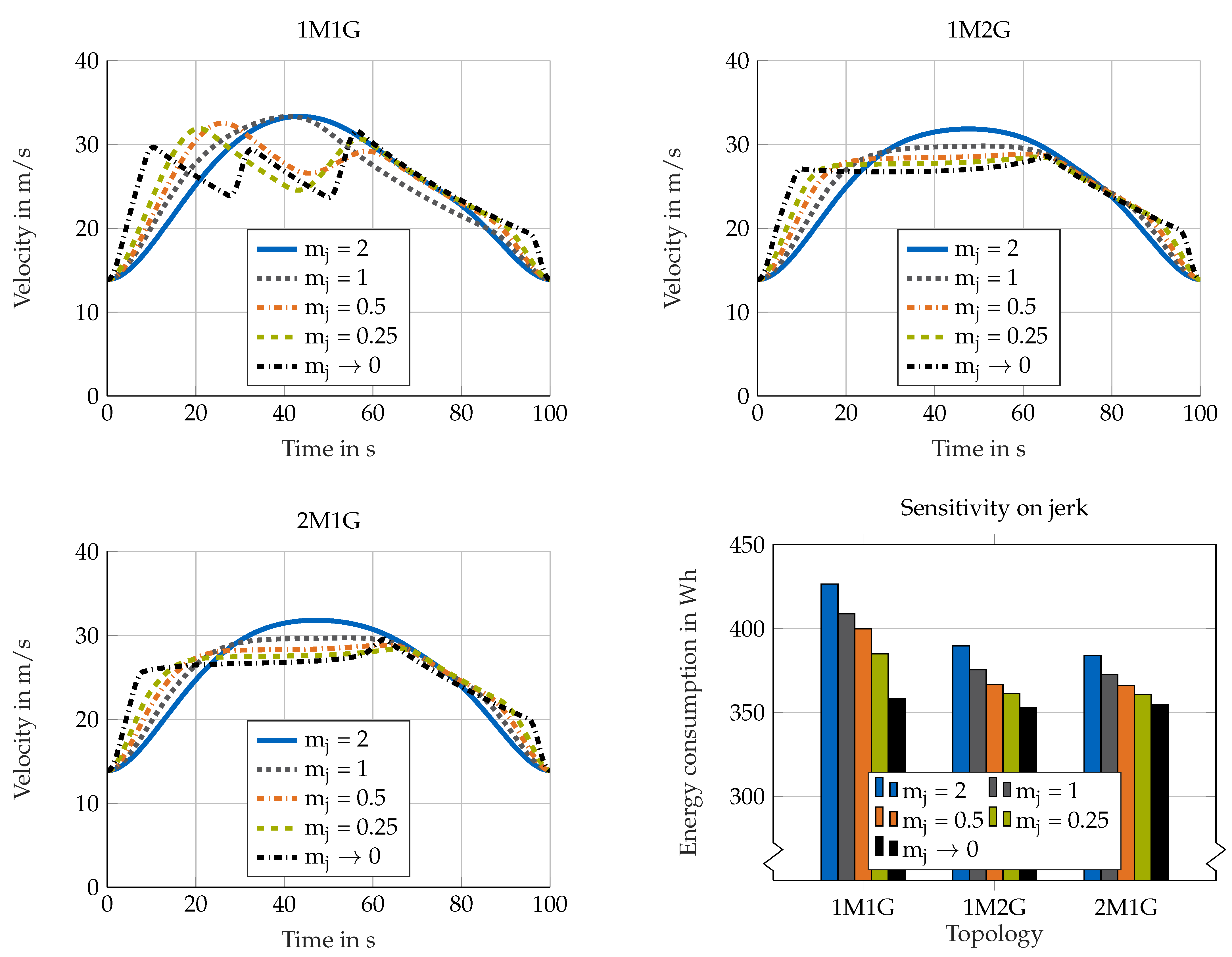
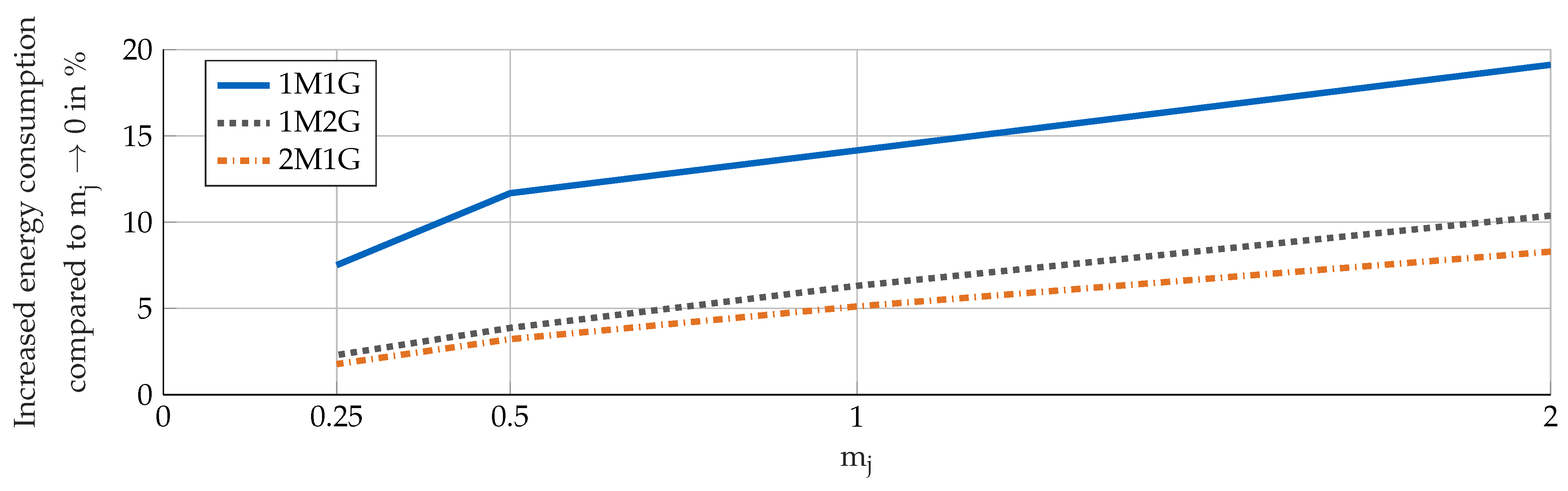
3.4. Sensitivity Analysis: Energy-Efficiency vs. Jerk

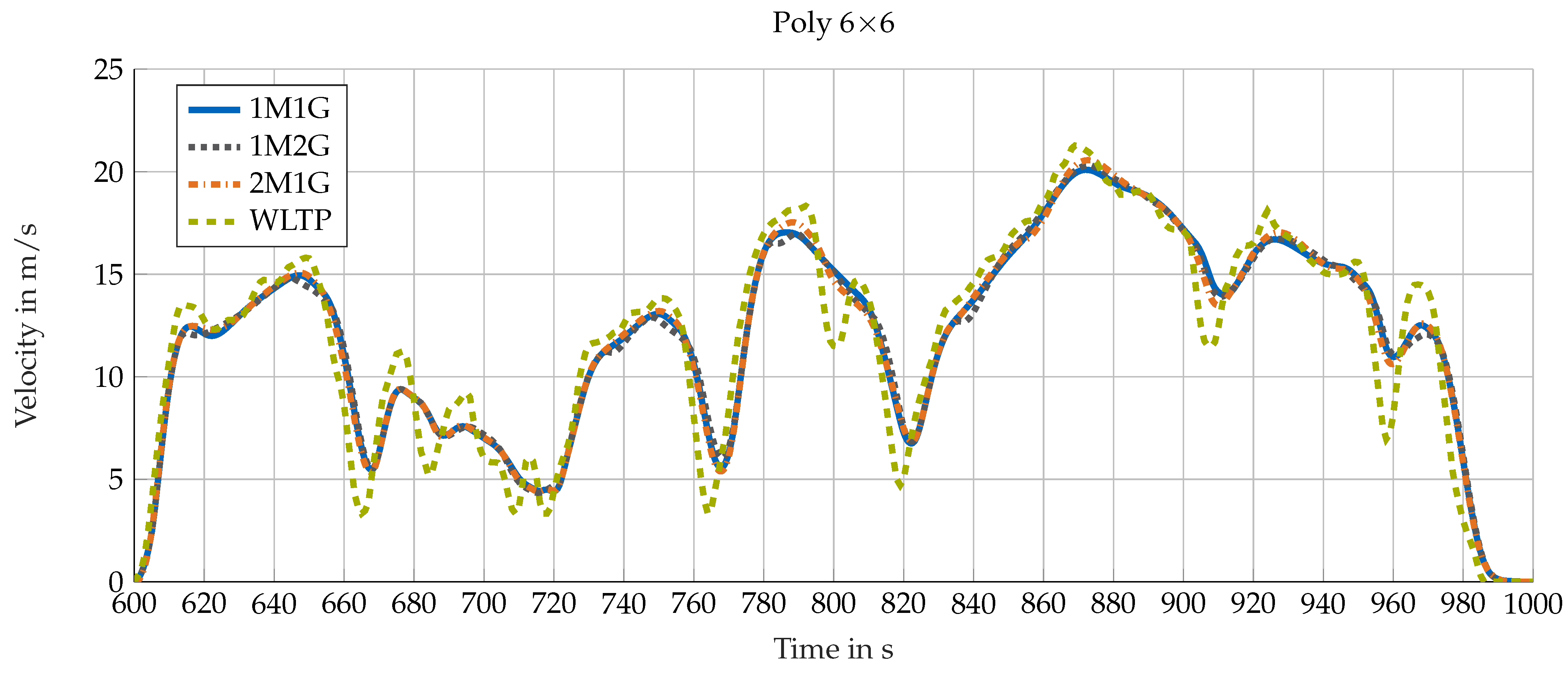
To see the interdependency between energy consumption and jerk limitation, further simulations using Poly 6 × 6 are conducted, where the global limitation on jerk is scaled by the factor $\frac{1}{m_j}$ (Equation (13)). Thus, if $m_j>1$, the jerk limitation gets stricter while an decreasing factor gives the optimization more freedom to reduce energy consumption. Figure 5 shows speed profiles for different levels of jerk restriction in the C2C scenario for 1M1G, 1M2G and 2M1G respectively as well as the final energy consumption. It can be seen that 1M1G tends to P&G if jerk is less restricted. The other topologies tend to accelerate, keep a constant speed and end with a gliding phase and hard braking. The gradients in the speed profiles get steeper if jerk is less restricted. Furthermore, a second pulse at $t\approx 65\mathrm{s}$ before the gliding phase can be seen if jerk is not restricted.

The relative difference in energy consumption compared to $m_j\to 0$ for different restrictions on jerk are shown in Figure 6. It can be seen that the energy consumption rises for higher restrictions on jerk. In particular, the 1M1G-topology increases energy consumption if jerk restrictions are rising. However, if no restriction is active, energy consumption of the 1M1G topology is almost as low as the energy consumption of the other topologies (Figure 5). Since the energy consumption for the 1M1G topology is higher if jerk is restricted, the sensitivity on jerk is higher for this topology.

3.5. Car-Following

The free-flow scenario was used to examine the general effects of eco-driving for various powertrain topologies. However, for more realistic results, a car-following scenario is implemented representing stricter boundary conditions. Figure 7 shows the different resulting speed profiles as well as the original speed of the WLTP. It can be seen that Poly 6 × 6 smooths the speed profiles, avoiding unnecessary accelerations. Furthermore, it includes coasting phases. The optimized speed profiles differ slightly in maximum speed between the powertrain topologies.

Table 5. Car-following results.

Algorithm/Cycle		1M1G	1M2G	2M1G
WLTP	Abs. in kWh	3.24	2.95	3.0
Poly 1 × 2	Abs. in kWh	3.17	3.16	3.29
	Rel. difference to WLTP in %	−2.4	+7.2	+9.7
Presented Poly 6 × 6	Abs. in kWh	3.12	2.82	2.85
	Rel. difference to WLTP in %	−3.7	−4.5	−5
	Rel. difference to Poly 1 × 2 in %	−1.4	−10.9	−13.4

shows the absolute energy consumption for different powertrain topologies using different algorithms and the relative difference in the WLTP and Poly 1 × 2 consumption of the examined powertrain topology. Likewise the C2C scenario, the Poly 1 × 2 is not able to reduce energy demand by the same extend like the Poly 6 × 6 algorithm. For the 2M1G topology, energy consumption increases with Poly 1 × 2 in comparison to 1M1G. With Poly 6 × 6, energy savings are between 3.7 and 5 percent towards the energy required driving the original WLTP with the corresponding powertrain. Again, energy consumption of the multi-speed and multi-motor topologies are lower compared to 1M1G. In comparison to the C2C scenario, the 1M1G topology has the lowest savings due to eco-driving.

4. Discussion

First, the results are discussed, followed by the proof of global optimality due to the comparison to DP. The section closes with the limitations and future work.

4.1. Discussion of Results

The results of the C2C scenario and car-following scenario (Section 3.3 and Section 3.5) show that the optimal speed profile and energy savings due to eco-driving depends on the powertrain configuration in an electric vehicle.

For the 1M1G topology, the speed profile consists of an acceleration, a coasting and a braking phase. Constant speed is avoided with the 1M1G topology, since this leads to low torque and thus low efficiency. Therefore, the vehicle accelerates to a higher speed and has a longer coasting phase. Although the higher speed increases the power loss due to air resistance, the better utilization of the motor map results in lower energy consumption.

For the 1M2G and 2M1G topology there is a quasi-constant speed phase after the acceleration. The second gear with the low gear ratio allows an efficient operation at constant speed. The same applies to the second motor. Due to the second, smaller motor, relatively high loads and thereby a high efficiency is achieved while cruising. With the ability to optimize the load point internally in the powertrain, the 1M2G and 2M1G topologies have lower energy consumptions than the 1M1G topology.

The sensitivity analysis (Section 3.4) shows the influence of jerk on energy consumption. For all topologies, a reduction in jerk leads to an increase in energy consumption. Vice versa, energy consumption can be reduced by reducing jerk restrictions. This can be explained by the fact that restricting jerk suppresses the fast setting of an efficient load point. As a result, vehicles operate longer with poor efficiency. However, the sensitivities vary between the topologies. While the consumption of the 1M1G topology varies by 19.1% in the considered scenarios, the consumption of the 1M2G and 2M1G topologies varies by 10.4% and 8.3%. Again, this can be explained by the possibility of powertrain-internal optimization. If a jerk limitation prevents a quick set up of an efficient load point, it is possible for the 1M2G and 2M1G topologies to drive more efficiently by using correct gear selection or correct load distribution. If, on the other hand, there is no jerk limitation, any powertrain topology can quickly set an efficient load point, resulting in almost equal energy consumptions among the topologies. If no comfort is considered, the speed profile of the 1M1G topology results in P&G, similar to Reference [12]. This is energy optimal but unrealistic for passenger trips. Penalizing or restricting jerk partially suppresses this behavior. The other topologies include a cruising phase, even if jerk is not restricted.

The potential savings due to eco-driving depend on the combination of scenario, powertrain and the reference speed profile. For the C2C scenario, the 1M1G topology has the highest relative savings, while for the car-following, the 2M1G topology has the highest relative savings. Optimizing the speed profile means optimizing the operating points. Thus, powertrains that were previously operated in poor operating points benefit more than powertrains that were operated at high efficiency during reference.

It was also shown that state-of-the-art optimization methods, here represented as Poly 1 × 2, optimizing “tank-to-distanc” efficiency, do not suffice for an simultaneous optimization of speed and powertrain operation for electric powertrains with multiple motors or gears due to an imprecise representation of the motor efficiency. Since the regions of best efficiency differ, the optimization chooses the wrong gear and wrong motor which may result in an increased energy demand. As the state of the art fits the electrical power by a quadratical function and minimizing it, low torques are preferred. However the original efficiency map reveals low efficiency for low torques. Thus, in this area the electrical power over torque is non-convex. The minimization of the real electrical power does prefer high torque or zero torque, which results in the typical P&G behavior.

The car-following scenario was solved on a laptop with an Intel Core i7-7820HQ with 16 GB of RAM. The average solving time for Poly 6 × 6 is 72 ms for the 1M1G topology. The 1M2G topology needs 121 ms for the relaxed problem and 62 ms for the actual problem. For the 2M1G topology, an average solving time of 137 ms is achieved. Thus, the algorithm is online capable. The Poly 1 × 2 algorithm needs 68 ms for the 1M1G topology.

4.2. Numerical Proof of Global Optimality

The results of the Poly 6 × 6-NLP are compared to the results of the DP, which calculates the global optimal solution within the discrete solution space. Figure 8 displays the resulting speed profiles of the DP and NLP with Poly 6 × 6 as well as the resulting motor torques for the 1M1G, 1M2G and 2M1G topology, respectively.

Likewise, the NLP’s optimal speed profiles, the DP’s optimal speed profiles differ among the different topologies. For the 1M1G topology, the speed profile consists of acceleration, coasting and braking. The other topologies include a quasi-constant speed phase. The acceleration phase for the DP and NLP differ for the 1M1G topology: At $t\approx 20\mathrm{s}$, the DP solution reduces acceleration and motor torque and keeps it constant for a longer time than the NLP. As a result, the top speed is slightly lower and the coasting phase for the DP is shorter. However, the final energy consumption, calculated by the original efficiency map, as in all our experiments, is only 0.9% higher for the NLP, in comparison to the DP. The speed profiles of NLP and DP for the 1M2G and 2M1G topologies are overlapping by a great extent. The energy consumption differs by 0.4% and 0.2%, respectively. The 1M2G topology optimized by DP shifts faster to the second gear ($t\approx 11\mathrm{s}$) and has a shorter coasting phase ($t\approx 71\mathrm{s}$). The 2M1G topology only uses the second motor for both solutions. Again, the coasting phase of the 2M1G topology is shorter ($t\approx 75\mathrm{s}$).

Even though there are differences between DP and NLP, the general behavior like the different segments in the speed profile as well as the general behavior of the chosen gear and chosen motor comply. Additionally, the final energy consumption coincide within 1% for all topologies. Differences can be explained by the discretization of the DP and the efficiency map fit of the NLP. Thus, it can be said that the behavior of the Poly 6 × 6-NLP is valid.

4.3. Limitations and Future Work

So far, only a static gear efficiency and the load-dependent motor efficiency have been considered. The gear efficiency could be modeled load-dependent, too. In addition, the modeling of the power electronics and the battery are further possibilities for improving the algorithm’s accuracy. These can all be combined into one map, which is then fitted. In addition, a more precise modeling of the idling torques of the different motor types may be useful. The algorithm is based on state-of-the art vehicle modeling equations and uses a motor efficiency map of a validated tool. With 13.9 kWh/100 km (neglecting auxiliary power) for the 1G1M topology, the simulation’s results are reasonable. However, future work should focus on the validation of the results. Tests on a dynamo-meter, similar to Reference [18] or the integration of the algorithm in other validated tools should be addressed.

It should be considered that the powertrains shown are not optimized. This means that adjusting the motor size and gear ratio can result in further savings. However, this algorithm allows the optimization of the powertrain considering different topologies and motors under realistic conditions. Thus, it may contribute to an extension of the solution space and the consideration of realistic scenarios for the powertrain optimization of CAVs, compared to References [3,4,5].

The first presented case study represents a free-flow scenario, without any disturbing traffic, the second represents a car-following scenario, in which the vehicle has to consider a leading vehicle. Traffic measures, like traffic lights and speed limits are spatial based characteristics but the presented algorithm is implemented in time domain. Thus, both scenarios had to be simplified. The scenarios do have a constant speed limit and no spatial based speed restrictions due to corners are implemented. For more realistic scenarios the algorithm can be called iteratively or can be implemented in the spatial domain. The algorithm’s integration in existing, validated simulation tool boxes allows more complex scenarios and powertrain simulations.

5. Conclusions

It has been shown that current online-capable eco-driving algorithms are not capable of optimizing speed and powertrain operation for electric vehicles with multiple gears and motors. In addition, current algorithms greatly overestimate motor efficiency at low torque, resulting in sub-optimal speed profiles. We presented an eco-driving algorithm that allows simultaneous optimization for multiple motors and gears. Furthermore, the efficiency at low torque is realistically represented. The test in a free-flow scenario and a car-following scenario show the savings potential of several motors and gears in an electric vehicle, including eco-driving. Depending on the scenario, optimal speed profiles differ for various powertrain topologies. In addition, the influence of jerk on energy consumption was shown. The comparison to Dynamic Programming shows valid behavior for the presented algorithm.

References

1. Eurostat. Final Energy Consumption in Road Transport by Type of Fuel. 2018. Available online: https://ec.europa.eu/eurostat/databrowser/view/ten00127/default/table?lang=en (accessed on 1 July 2020).
2. Kopelias, P.; Demiridi, E.; Vogiatzis, K.; Skabardonis, A.; Zafiropoulou, V. Connected & autonomous vehicles—Environmental impacts—A review. Sci. Total Environ. 2020, 712, 135237. [Google Scholar] [CrossRef] [PubMed]
3. Anselma, P.G.; Belingardi, G. Enhancing Energy Saving Opportunities through Rightsizing of a Battery Electric Vehicle Powertrain for Optimal Cooperative Driving. SAE Int. J. Connect. Autom. Veh. 2020, 3. [Google Scholar] [CrossRef]
4. Tate, L.; Hochgreb, S.; Hall, J.; Bassett, M. Energy Efficiency of Autonomous Car Powertrain; SAE Technical Paper Series; SAE International400 Commonwealth Drive: Warrendale, PA, USA, 2018. [Google Scholar] [CrossRef]
5. Ullekh Raghunatha Gambhira. Powertrain Optimization of an Autonomous Electric Vehicle. Master’s Thesis, The Ohio State University, Columbus, OH, USA, 2018.
6. Christian Angerer. Antriebskonzept-Optimierung für Batterieelektrische Allradfahrzeuge. Ph.D. Thesis, Technische Universität München, München, Germany, 2020.
7. Vaillant, M. Design Space Exploration zur Multikriteriellen Optimierung Elektrischer Sportwagenantriebsstränge. Ph.D. Thesis, Karlsruher Institut für Technologie, Karlsruhe, Germany, 2015. [Google Scholar]
8. Hofman, T.; Dai, C. Energy efficiency analysis and comparison of transmission technologies for an electric vehicle. In Proceedings of the 2010 IEEE Vehicle Power and Propulsion Conference, Lille, France, 1–3 September 2010; pp. 1–6. [Google Scholar]
9. Pesce, T. Ein Werkzeug zur Spezifikation von Effizienten Antriebstopologien für Elektrofahrzeuge. Ph.D. Thesis, Doktorhut, München, Germany, 2014. [Google Scholar]
10. Sciarretta, A. Energy-Efficient Driving of Road Vehicles: Toward a Cooperative, Connected, and Automated Mobility; Springer International Publishing: Berlin/Heidelberg, Germany, 2019. [Google Scholar] [CrossRef]
11. Mensing, F.; Trigui, R.; Bideaux, E. Vehicle trajectory optimization for application in ECO-driving. In Proceedings of the 2011 IEEE Vehicle Power and Propulsion Conference, Chicago, IL, USA, 6–9 September 2011; pp. 1–6. [Google Scholar]
12. So, K.M.; Gruber, P.; Tavernini, D.; Karci, A.E.H.; Sorniotti, A.; Motaln, T. On the Optimal Speed Profile for Electric Vehicles. IEEE Access 2020, 8, 78504–78518. [Google Scholar] [CrossRef]
13. Teichert, O.; Koch, A.; Ongel, A. Comparison of Eco-Driving Strategies for Different Traffic-Management Measures. In Proceedings of the 2020 IEEE Intelligent Transportation Systems Conference (ITSC), Rhodes, Greece, 20–23 September 2020; pp. 1867–1873. [Google Scholar]
14. Han, J.; Vahidi, A.; Sciarretta, A. Fundamentals of energy efficient driving for combustion engine and electric vehicles: An optimal control perspective. Automatica 2019, 103, 558–572. [Google Scholar] [CrossRef]
15. Dollar, R.A.; Vahidi, A. Quantifying the impact of limited information and control robustness on connected automated platoons. In Proceedings of the 2017 IEEE 20th International Conference on Intelligent Transportation Systems (ITSC), Yokohama, Japan, 16–19 October 2017; pp. 1–7. [Google Scholar] [CrossRef]
16. Zhang, C.; Vahidi, A. Predictive cruise control with probabilistic constraints for eco driving. In Proceedings of the Dynamic Systems and Control Conference, Arlington, VA, USA, 31 October–2 November 2011; Volume 54761, pp. 233–238. [Google Scholar]
17. Wegener, M.; Plum, T.; Eisenbarth, M.; Andert, J. Energy saving potentials of modern powertrains utilizing predictive driving algorithms in different traffic scenarios. Proc. Inst. Mech. Eng. Part D J. Automob. Eng. 2020, 234, 992–1005. [Google Scholar] [CrossRef]
18. Eo, J.S.; Kim, S.J.; Oh, J.; Chung, Y.K.; Chang, Y.J. A Development of Fuel Saving Driving Technique for Parallel HEV; SAE Technical Paper Series; SAE International400 Commonwealth Drive: Warrendale, PA, USA, 2018. [Google Scholar] [CrossRef]
19. Li, S.E.; Peng, H. Strategies to minimize the fuel consumption of passenger cars during car-following scenarios. Proc. Inst. Mech. Eng. Part D J. Automob. Eng. 2012, 226, 419–429. [Google Scholar] [CrossRef]
20. Shao, Y. Optimization and Evaluation of Vehicle Dynamics and Powertrain Operation for Connected and Autonomous Vehicles; Dissertation, University of Minnesota Digital Conservancy. 2019. Available online: http://hdl.handle.net/11299/211322 (accessed on 28 December 2020).
21. Guo, L.; Gao, B.; Gao, Y.; Chen, H. Optimal Energy Management for HEVs in Eco-Driving Applications Using Bi-Level MPC. IEEE Trans. Intell. Transp. Syst. 2017, 18, 2153–2162. [Google Scholar] [CrossRef]
22. Qi, X.; Wu, G.; Hao, P.; Boriboonsomsin, K.; Barth, M.J. Integrated-Connected Eco-Driving System for PHEVs with Co-Optimization of Vehicle Dynamics and Powertrain Operations. IEEE Trans. Intell. Veh. 2017, 2, 2–13. [Google Scholar] [CrossRef] [Green Version]
23. Li, L.; Wang, X.; Song, J. Fuel consumption optimization for smart hybrid electric vehicle during a car-following process. Mech. Syst. Signal Process. 2017, 87, 17–29. [Google Scholar] [CrossRef]
24. Li, Y.; Wu, D.; Du, C.; Yang, H.; Li, Y.; Yang, X.; Lu, X. Velocity Trajectory Planning for Energy Savings of an Intelligent 4WD Electric Vehicle Using Model Predictive Control; SAE Technical Paper Series; SAE International400 Commonwealth Drive: Warrendale, PA, USA, 2018. [Google Scholar] [CrossRef]
25. Lelouvier, A.; Guanetti, J.; Borrelli, F. Eco-platooning of autonomous electrical vehicles using distributed model predictive control. Parameters 2017, 2, 4. [Google Scholar]
26. Murgovski, N.; Johannesson, L.; Sjöberg, J. Convex modeling of energy buffers in power control applications. IFAC Proc. Vol. 2012, 45, 92–99. [Google Scholar] [CrossRef] [Green Version]
27. Padilla, G.; Weiland, S.; Donkers, M. A global optimal solution to the eco-driving problem. IEEE Control Syst. Lett. 2018, 2, 599–604. [Google Scholar] [CrossRef]
28. Guzzella, L.; Sciarretta, A. Vehicle Propulsion Systems: Introduction to Modeling and Optimization, 3rd ed.; Springer: Berlin/Heidelberg, Germany, 2013. [Google Scholar] [CrossRef]
29. Mitschke, M.; Wallentowitz, H. Dynamik der Kraftfahrzeuge; Springer Fachmedien Wiesbaden: Wiesbaden, Germany, 2014. [Google Scholar] [CrossRef]
30. Marler, R.T.; Arora, J.S. The weighted sum method for multi-objective optimization: New insights. Struct. Multidiscip. Optim. 2010, 41, 853–862. [Google Scholar] [CrossRef]
31. Andersson, J.A.E.; Gillis, J.; Horn, G.; Rawlings, J.B.; Diehl, M. CasADi—A software framework for nonlinear optimization and optimal control. Math. Program. Comput. 2019, 11, 1–36. [Google Scholar] [CrossRef]
32. Wächter, A.; Biegler, L.T. On the implementation of an interior-point filter line-search algorithm for large-scale nonlinear programming. Math. Program. 2006, 106, 25–57. [Google Scholar] [CrossRef]
33. Mersky, A.C.; Samaras, C. Fuel economy testing of autonomous vehicles. Transp. Res. Part C Emerg. Technol. 2016, 65, 31–48. [Google Scholar] [CrossRef]
34. Kalt, S.; Erhard, J.; Lienkamp, M. Electric Machine Design Tool for Permanent Magnet Synchronous Machines and Induction Machines. Machines 2020, 8, 15. [Google Scholar] [CrossRef] [Green Version]
35. BMW. Technische Daten.Der neue BMWi3. 2017. Available online: https://www.press.bmwgroup.com/deutschland/article/attachment/T0273661DE/392973 (accessed on 9 July 2020).
Figure 1. Comparison of motor efficiency maps between original, Poly 1 × 2 and Poly 6 × 6 fit.
Wevj 12 00006 g001
Figure 2. Comparison of different optimization methods for a 1M1G topology (a) speed profiles (b) energy savings to a 2 minimization.
Wevj 12 00006 g002
Figure 3. Comparison of different topologies with Poly 6 × 6 (a) speed profiles (b) energy consumption.
Wevj 12 00006 g003
Figure 4. Comparison of different topologies with Poly 1 × 2 (a) speed profiles (b) energy consumption.
Wevj 12 00006 g004
Figure 5. Speed profiles and energy consumption for different jerk limits and topologies.
Wevj 12 00006 g005
Figure 6. Relative energy consumption for different jerk limits compared to m j 0 in %.
Wevj 12 00006 g006
Figure 7. Optimized speed profiles for different topologies and original worldwide harmonized light vehicles test procedure (WLTP).
Wevj 12 00006 g007
Figure 8. Comparison of Dynamic Programming (DP) and nonlinear programming (NLP) for city to city (C2C) scenario.
Wevj 12 00006 g008