Cloud-Based Big Data Platform for Vehicle-to-Grid (V2G) ^†

Abstract

Battery Electric Vehicles (BEVs) have increasingly become prevalent over the past years. BEVs can be regarded as a grid load and as a way to support the grid (energy buffering), provided this extensive battery usage does not affect the BEV’s performance. Data from both the vehicle and the grid are required for effective Vehicle-to-Grid (V2G) implementation. As such, a cloud-based big data platform is proposed in this paper to exploit these data. Additionally, this study aims to develop smart algorithms, which optimise different factors, including BEV cost of ownership and battery degradation. Dashboards are developed to provide key information to different V2G stakeholders.

1. Introduction

The penetration of Battery Electric Vehicles (BEV) has been faster than expected in part due to a recent diesel emission scandal and decreasing battery price. A KPMG report [1] highlighted that BEVs would be between 11–15% of new vehicle sales within EU and China by 2025. Within the UK, the market will comprise 16–20% of vehicles over the next 10 years. Several Original Equipment Manufacturers (OEM) have aligned themselves with these projections: Volkswagen Group planned to release 80 new variants of BEV by 2025, Volvo announced that after 2019 all vehicles would be partially or completely battery-powered, and Ford will introduce 13 new BEV models over the next 5 years. Due to the low energy density of the battery, BEV users have concerns when the battery is reaching its bottom level and whether next charging station is available and in the proximity. Even though the number of charging station is increasing rapidly, it would be a challenge to meet rapid BEV penetration. For example, it is predicted to be 1 million electric vehicles on the road in the UK by 2020s, which is 10 times greater than the current number of vehicles. The charging infrastructure must increase by at least the same amount to maintain similar service [2]. The expansion of the charging stations must be in adequation to the customer’ needs. Quddus et al. [3] proposed a model for this expansion, considering the integration of renewable energies.

One drawback of BEV penetration is the increasing load on the electrical grid during the peak hours when BEVs are charging. Two solutions exist; increase the grid capacity or develop smart charging. The first solution is expensive, while the second one, easier to implement, requires better charging management [4,5,6,7,8]. In addition to smart charging, Vehicle-to-Grid (V2G) offers the possibility for BEVs to support the grid owing to their large-capacity battery. The benefits of V2G have yet to be fully explored and communicated to stakeholders, including BEV owners, vehicle manufacturers, energy suppliers and government. Yilmaz and Krein [9] and Ehsani et al. [10] proposed a wide review of the V2G potential benefits and applications. OEMs could integrate, in their future BEV models, built-in V2G capability, including a bi-directional charging system. Charging stations could allow bi-directional power flow, and, finally, utility companies could define the battery energy selling price. Recent reports highlight the V2G charger market will grow at a Compound Annual Growth Rate (CAGR) of 50.05% during the period of 2018-2022 [11]. Each BEV connected to the grid could be used as bidirectional energy storage – storing renewable energy when available and releasing that energy during peak demand [12]. The peak shaving capability and benefits enabled by V2G have been emphasised by Aziz et al. [13] and Li et al. [14]. A research thesis by Kaufmann [15] estimates the financial return from V2G could be circa $1275 per vehicle every year, while the NREL claimed in 2015 that circa $1825 per vehicle every year is achievable.

V2G with high BEV penetration could provide new opportunities and threats to the electricity market. As stated in “Electric Vehicles” IRENA report [16], there is a potential for the electricity market to adopt structures and a regulatory framework that enables V2G business models to decarbonise the grid, improve efficiency and mitigate the need for grid-reinforcement. The willingness for the population to adopt BEV and V2G is crucial. Some surveys and studies focus on this willingness, especially in Northern Europe countries [17,18,19]. They highlight the need for clear government positions and regulations. Wang et al. [20] introduced a rewarding scheme based on blockchain, which could encourage the willingness for V2G adoption. Increased percentage penetrations of wind and solar will underpin a greater need for V2G to both optimise the integration of these resources and to balance frequency disturbances created from their variability in a generation [21,22,23]. According to Navigant Research, frequency regulation revenue will reach $190.7 million by 2022 [24].

Previous projects considered an optimisation approach to enable V2G. In Nguyen and Le’s analysis [25], optimisation is done on BEV and home energy scheduling. The goal is to minimise electricity cost and user discomfort. Another study aims to minimise the plug-in electric vehicle charging cost proposing six algorithms [26]. The battery supporting the grid will operate more often than battery only used for vehicle propulsion. Those extra battery cycles may lead to faster battery degradation [27]. In Wang et al. analysis [28], a minor lifetime reduction is observed. Another study [29] analysed the profitability of V2G, considering battery degradation. It concluded that considering energy prices and battery costs, V2G is not currently profitable for BEV owners, but the expected battery cost reduction could provide benefits to future BEV owners. V2G could be an opportunity to introduce dynamic electricity pricing, as discussed in [30]. The majority of the aspects of V2G have been studied separately in different previous research works. However, for a fully functional V2G system, all aspects must be considered at the same time on a common platform, which this work is addressing.

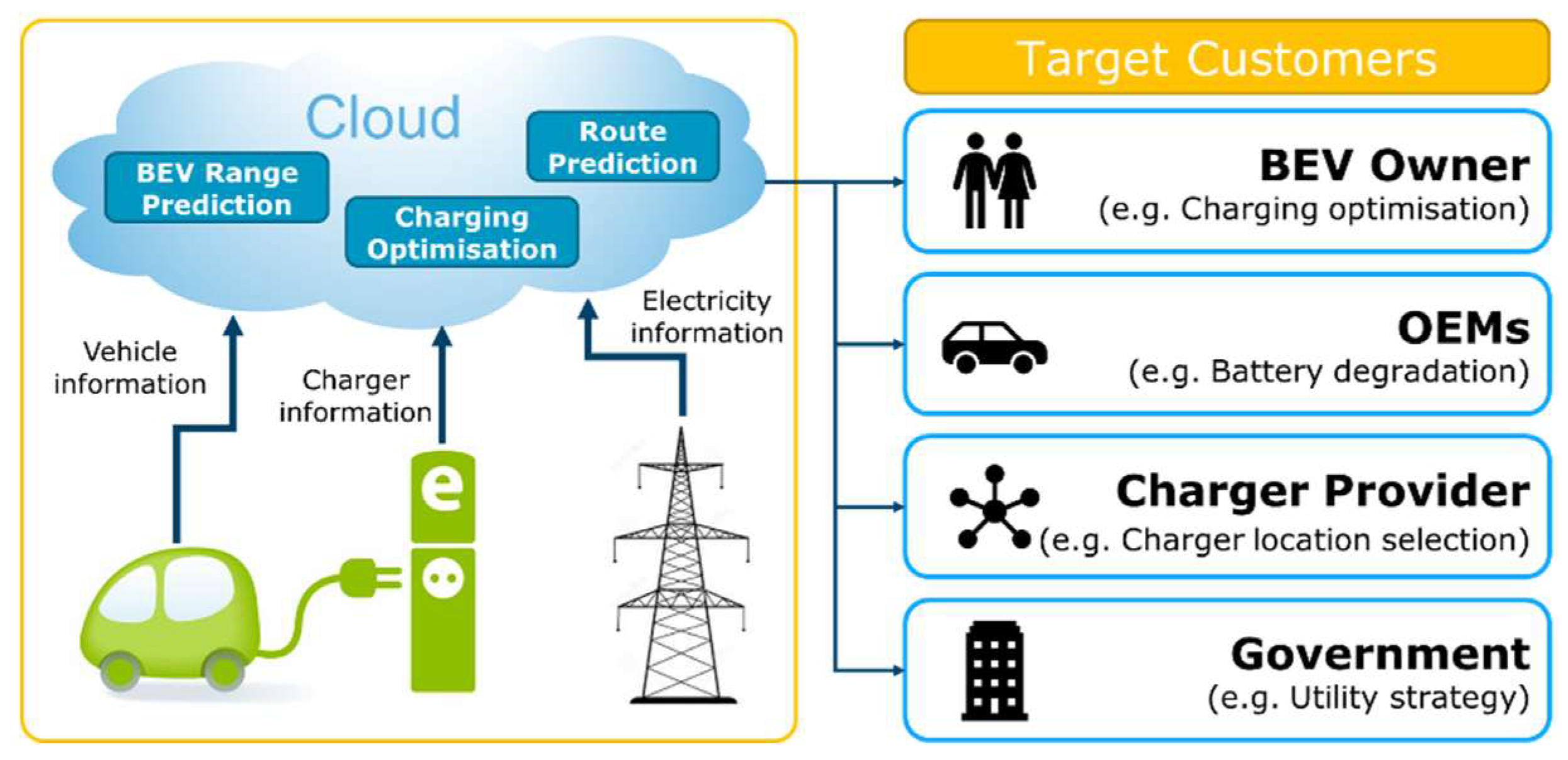
In this paper, the aim is to optimise the charging cost and battery degradation for BEV using Dynamic Programming (DP). In the rest of the paper, “charging optimisation” refers to charging and discharging optimisation based on electricity cost and battery degradation. Before performing the optimisation, smart algorithms using machine learning are developed to predict whether the vehicle will be plugged in, the charging duration, the next trip destination, the next trip distance, and the next trip energy required. The novelty lies in the usage of a cloud-based platform and the data-driven approach adopted. Until BEV range becomes sufficiently high or charging stations become as prevalent as gas stations, data from vehicles and charging stations will continue to play a key role in mitigating range anxiety. These data can be stored in the cloud and enriched with additional sources, such as electrical grid information and battery degradation model, for further analytics. Once the creation of the integrated database is ready, it could be used for various purposes. BEV owners, for instance, could reap the benefit of the charging optimisation by reducing electricity cost, and OEMs could use this database to understand how battery degradation would differ with various charging and driving behaviours. Charging station providers could utilise this database to design charging infrastructure to provide a better service to BEV owners. For government or utility providers, the database can enhance understanding of electricity load and mitigate electricity load issues due to high electricity demand from BEV. Figure 1 illustrates the V2G data platform and its potential users.

The key objective of this paper is to develop state-of-the-art V2G analysis tools and model for:

(1)

the creation of a smart data collection and management infrastructure, and

(2)

advanced analytics, including charging optimisation.

As data format from vehicle and grid is different, it is important to convert and combine these data into a common format. A Not only Structured Query Language (NoSQL) database is used due to its flexibility and capability to deal with this type of data. The database is implemented in the cloud in order to reduce memory and computation burden on the vehicle or on the On-Board Charger (OBC). Based on the data stored, algorithms, such as route prediction, BEV range prediction and charging optimisation, have been developed. Finally, the results are shared with target customers via an online dashboard.

The second section of this article details the data pipeline with information about data logging and enrichment. The database characteristics are also discussed, as well as cloud architecture. The third section explains the development of the algorithms, the way they work and implementation output. The fourth and penultimate section highlights analysis results and topics to investigate further, before conclusion remarks.

2. Materials and Methodology

For this research, real-world data from 15 vehicles and more than 5000 trips over 1 year have been logged internally (Figure 2). Data loggers are installed via vehicle On-Board Diagnostics (OBD) port, and CAN data are recorded and transferred to Secure FTP (SFTP) server. These data are pre-processed in terms of data quality, consistency check and data reformatting. The data on the individual contains the vehicle speed, GPS coordinates, ambient temperature, date and time. The driver identity, home and work addresses and vehicle type are not collected to ensure driver’s privacy. The approach detailed in this manuscript requires the GPS position at the start and end of the trip. BEV GPS positions are logged for optimisation purposes only and not shared for any other purpose. Drivers that do not want to be tracked by GPS would not benefit from this solution. Vehicle information is used to create the metadata and merged with vehicle time-series data, forming the primary data for the database. Some important information, such as electricity cost and charger information (i.e., location, power), cannot be logged by the datalogger; hence external sources are required to enrich the database. This database is additionally enriched with secondary information, constituting electricity cost and charger information, both of which come from external sources (e.g., Google Application Programming Interface (API), HERE API).

The electricity cost is averaged after gathering the prices from the “Big Six” in the United Kingdom (British Gas, EDF, E. ON, npower, SSE, Scottish Power). One and two rate tariffs are taken into account, making the price ranging from GBP (pound sterling) 0.162/kWh to GBP 0.197/kWh. There is currently no tariff when selling the BEV electricity to the grid in the UK. However, at the beginning of 2010s, the electricity generated by individuals from photovoltaic panels was sold at GBP 0.44/kWh to the grid. Based on this information, the price for selling to the grid is assumed to be from GBP 0.25/kWh to GBP 0.45/kWh to consider both single and two rate tariffs. The charger information is queried from API, such as HERE (https://www.here.com/) or OpenChargeMap (https://openchargemap.org/site), where GPS coordinates and charging power are extracted. As V2G compatible chargers are not available at commercial scale, it is assumed that all chargers are reversible and allow V2G.

At this stage, all the data are available and need to be stored in a database. Two database types have been considered for this study: Structured Query Language (SQL) and Not only SQL (NoSQL). SQL is often used to store a relational database in a table format, while NoSQL is not limited to rows in a table and thus supports a non-relational database. NoSQL is schema-free as it consists of documents with different formats: time-series, string and single value. NoSQL is selected for this research due to its high flexibility and scalability [31]. MongoDB is the database program chosen to support the database owing to its capability to store data in JSON-like documents and its compatibility with Python.

Smart algorithms have been first developed on local machines before being pushed to the cloud. They can benefit from the computation power of the cloud and hence remove the need for embedded computation capabilities in the vehicle. Microsoft Azure is the cloud solution chosen. A Windows-based virtual machine is created where the database is synchronised with an on-premises server database (MongoDB). On the on-premises server-side, the database is uploaded to a Blob storage service via a script. Blob storage is a Microsoft Azure service for data storage in the cloud, and it can store any type of data, such as photos, videos, texts, etc. Then, on the cloud, the opposite process is done with another script that downloads the database from Blob storage. The smart algorithms, initially developed locally, are run in the cloud, and their outputs are stored in the database (Figure 3). The calculation outputs are analysed, and dashboards are created to visualise the results. A Power BI Gateway is required in order to make the data available online. Three PowerBI dashboards are created, considering different targets: the BEV owners, the charger providers/utility companies and the OEMs.

3. Development and Results

Once the database is ready, it can be used with algorithms. As mentioned in the previous section, depending on the stakeholder, analytics may be different. In this paper, charging optimisation for BEV owners is investigated. Charging optimisation requires relevant information, such as next trip route prediction and next trip range, both required to set battery State-of-Charge (SOC) target. Figure 4 depicts the algorithm flow diagram. The various algorithms depicted are detailed in the next section. The database contains all the information required to control and predict the charging power for each vehicle. The only extra input required is the Vehicle Identification Number (VIN) in order to select the appropriate vehicle data for the algorithms.

The data are logged from conventional vehicles. Hence, as part of the data pre-processing, these data must be converted to BEV data. For this purpose, a BEV model, representing a C-segment vehicle with a 24 kWh onboard battery capacity, has been developed. The converted data, including battery power, SOC and average energy consumption, are then stored in the database for use as an input to the other algorithms.

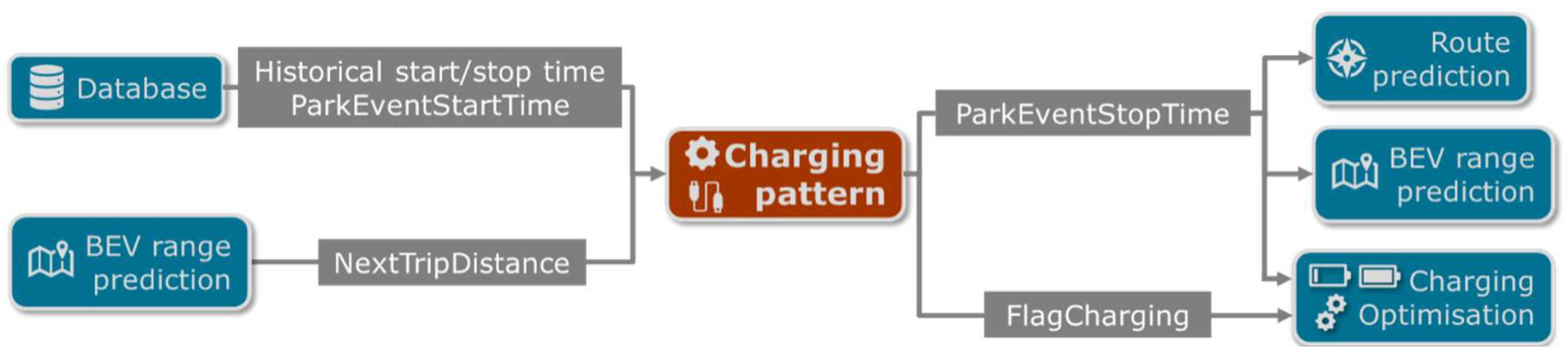
3.1. Charging Pattern Prediction

The charging pattern algorithm consists of two parts, as depicted in Figure 5. The objective of the first part of this algorithm is to predict the stop date and time of the parking event (ParkEventStopTime). The second part outputs a binary indicator of whether the vehicle is plugged in (i.e., charging) or not during the parking event (FlagCharging).

ParkEventStopTime is determined using the predicted duration of the parking event. This is a regression problem as the duration, which is an output, is a continuous value. As implemented in [32], feature importance is assessed to determine the significance of the various variables for predicting the output, which is parking duration in this case. The most important variables are found as start and stop location, start and stop time of the trip finished and a binary indication of either weekend or weekday. Parking duration prediction is then implemented and tested using both Decision Tree and Random Forest machine learning methods.

Decision Tree is an efficient machine learning approach for solving both regression and classification tasks. Random Forest is a collection of Decision Trees run in parallel and averaged to get a final prediction. The implementation details of both Decision Tree and Random Forest in this paper are depicted in

Table 1. Decision Tree and Random Forest implementation details.

Decision Tree		Random Forest
Property	Value	Property	Value
Tree induction algorithm	Classification and Regression Trees (CART)	Number of trees	100
Stopping criteria	Minimum samples split or minimum samples leaf	Model averaging method	Bootstrap aggregating
Information gain metric	Mean square error	Feature selection	Randomised
Cross-validation	80% of data set for training, 20% for validation	Cross-validation	80% of data set for training, 20% for validation

. For a more detailed treatment of these approaches, the reader is referred to [33].

Performance comparison between Decision Tree and Random Forest is evaluated using Mean Absolute Error (1) and by examining the correlation between true and predicted values of parking event duration.

$$MAE \left[h\right]=\frac{{{\displaystyle \sum }}_{i=1}^N\left|y_i-x_i\right|}{N},$$

(1)

where $y$ stands for real parking duration, $x$. is the predicted parking duration and $N$ is the number of observations in the test set. Results suggest that Decision Tree performs better than Random Forest according to the Mean Absolute Error and correlation coefficients between predicted and true values of parking event duration. Mean Absolute Errors are 2.39 and 2.91 h, and correlation coefficients between real and predicted values are 0.65 and 0.41, respectively.

Moving on to prediction of the charging indicator FlagCharging, researchers have examined the various factors, affecting the user’s choice of whether to charge a vehicle or not [34]. Prediction of a charging event is a binary classification type of problem, where output 0 refers to a vehicle not being plugged-in, output 1 refers to the vehicle being plugged-in. The next trip distance (as per Section 3.3) and parking duration are chosen to be the inputs.

The dataset used for determining FlagCharging is collected for My Electric Avenue (MEA) project [35]. This external dataset is used because it provides information on whether a vehicle is plugged in (i.e., charging) during a parking event or not. The input variables used for the predictive models adopted are start and stop time of the trips and start and stop time of charging events. Decision Tree and Random Forest machine learning models are then implemented on the MEA data as per Table 1.

Table 2. Charging prediction accuracy with different prediction methods.

Method	Decision Tree	Random Forest
Accuracy (%)	80.8	85.6

shows the accuracy results of both models, where accuracy is computed as the percentage of correct predictions among all predictions.

From the accuracy results in Table 2, Random Forest provides more accurate results compared to the Decision Tree. Thus, Random Forest is chosen as a final predictor of whether a vehicle is plugged-in or not.

3.2. Route Prediction

The aim of the algorithm described in this section is to predict next trip destination (NextTripDestination) using the vehicle’s current and historical locations, as well as the time at the end of a parking event, as depicted in Figure 6.

The route prediction problem in this paper is equivalent to a destination prediction problem. Destination prediction has been widely studied [36]. In this paper, potential destinations are first identified by examining locations of significance using a spatial clustering algorithm. Then, a Markovian approach is used for destination prediction.

The most challenging part of the clustering algorithm is geographical data pre-processing. The geographical data used consists of a sequence of destinations in the form $\left(x, y\right)$, where $x$ is latitude, $y$ is longitude. A commonly used algorithm for clustering is Density-Based Spatial Clustering of Applications with Noise (DBSCAN) [37], and this is the one selected here.

The DBSCAN algorithm requires two parameters: ε (epsilon) and $minPts$ (minimum number of points). It outputs two sets of points: cluster points and noise. The algorithm randomly selects one point (location in this case) and counts the number of points within ε around the selected point. If the number of counted points is at least equal to $minPts$, then a cluster is formed. The next step is to check if the criteria are met for other points inside the formed cluster; meaning that if we consider ε distance around each point inside the cluster and it is found that there are at least $minPts$ enclosed within ε, then the enclosed points are added to the cluster. Otherwise, a point that does not enclose $minPts$ within ε is defined as noise. This process is repeated until all points are classified as either within-cluster or noise. In Figure 7, blue points are shown to form a cluster, while green ones are classified as noise.

In this paper, the algorithm parameterisation is; $\mathsf{\epsilon }=0.3\mathrm{km}$ and $minPts=5$. This parameter choice is arrived at after examining various parameter values.

Table 3. DBSCAN (Density-Based Spatial Clustering of Applications with Noise) parameters definition.

$\mathit{\epsilon }$	% of Noise	# of Clusters
0.5	12.84	15
0.4	14.08	16
0.3	14.75	16

summarises this parameter variation where $minPts$ is arbitrarily fixed at 5. The parameter $\mathsf{\epsilon }$ is varied in steps of 0.1 km from 0.3 km to 0.5 km. The percentage of noise (“% of noise” column) represents the proportion of points that do not belong to any cluster. The smaller $\mathsf{\epsilon }$ is, the more points are defined as noise as there are not enough neighbours ($minPts$) within $\mathsf{\epsilon }$ to form a cluster. Also, the number of clusters increases with the reduction of $\mathsf{\epsilon }$. Clustering with $\mathsf{\epsilon }=0.3$ is adopted for further analysis after finding that it yields the most geographically relevant clustering using Google Maps, as shown in Figure 8.

Finally, now that all locations have been clustered into potential destinations, a Markovian approach is used for the destination prediction problem. The Markov chain method is used here, owing to its applicability to problems with sequential data [38]. The set of clusters form the state space for the Markov Chain, meaning that movement from one cluster to another is a transition between states. The following three steps give an overview of the implementation of the Markov chain method:

(1)

A sequence representing the movement of a vehicle between clusters (i.e., states) is established. Let $s=\left\{s_1,s_2,s_3,\dots ,s_r\right\}$ be the set of states that can be assumed.

(2)

Define the Transition Probability (TP) from state $s_i$ to state $s_j$ as $p_{ij}$. A TP matrix $S=\left(p_{ij}\right)$ is computed from historical data, where

$$p_{ij}=P\left(s_i\to s_j\right)=\frac{N\left(s_i\to s_j\right)}{{{\displaystyle \sum }}_{n=1}^{n=r}N\left(s_i\to s_n\right)},$$

(2)

(3)

If the start location is the cluster $i$, the $i$th row of the TP matrix is used to predict the next destination since the row represents probabilities of movement from cluster $i$ to all the other clusters.

The data used for calculating TP matrix are divided into “time-windows”, as proposed in [39,40,41]. This can be justified by the assumption that a person’s driving habits highly depend on the time of the day and the day of the week. For example, one may always drive from home to office between 7:00 am and 9:00 am on weekdays. The algorithm is tested on 1037 destinations of a vehicle. Results of the destination prediction algorithm can be seen in

Table 4. Destination prediction results for a weekday.

Metrics	Unit	Without Time Windows	Weekday (With Time Windows)
		n/a	06:00–10:00	10:00–12:00	12:00–14:00	14:00–16:00	16:00–20:00	20:00–23:00	23:00–06:00
# of points	(#)	1037	189	101	78	127	293	23	9
# of clusters	(#)	16	3	3	3	4	6	1	1
Accuracy	(%)	42	78	62.5	50	60	62	100	100
Mean distance error	(km)	4.5	4.4	0.2	0.3	0.3	0.7	0.01	0
Error	(%)	46.4	40.3	3.8	3.2	3.3	11.5	0	0

and

Table 5. Destination prediction results for the weekend.

Metrics	Unit	Without Time Windows	Weekend (With Time Windows)
		n/a	07:00–11:00	11:00–13:00	13:00–16:00	16:00–22:00	22:00–07:00
# of points	(#)	1037	37	46	59	63	12
# of clusters	(#)	16	1	2	2	2	1
Accuracy	(%)	42	100	100	71	86	100
Mean distance error	(km)	4.5	0	0.02	0.08	0.08	0.002
Error	(%)	46.4	0	0.1	0.8	0.6	0

.

The accuracy measures used in Table 4 and Table 5 are defined in the following equations:

$$A\mathit{ccuracy}[\%]=\frac{\#ofclusterspredictedcorrectly}{total\#ofpredictions}\times 100,$$

(3)

$$\mathit{Mean}\mathit{distance}\mathit{error}\left[\mathrm{km}\right]=\frac{{{\displaystyle \sum }}_1^N(DistReal-DistPredicted)}{total\#ofpredictions},$$

(4)

$$\mathit{Error}[\%]=\frac{Mean distanceerror}{Average trip distance}\times 100.$$

(5)

Equation (3) represents the amount of correctly predicted clusters over the whole set of clusters as a percentage. Equation (4) stands for mean distance error, which is an average difference in distances between real destination and the predicted one, in kilometres. Equation (5) is a proportion of mean distance error over average trip distance, in percentage.

The results in Table 4 and Table 5 confirm the benefits of dividing the prediction into different time-windows. Without time-windows, the prediction accuracy is 42%. With time-windows, the prediction accuracy is always more than 50% for weekdays and at least 71% for the weekend. It can go up to 100% in some cases. The weekday (with time window) in Table 4 has one large mean distance error occurring from 06:00–10:00. This has been found to be due to a rarely driven route, affecting the metric calculation in the end.

Note that for destination prediction, it is assumed that only destinations present in the available data will be reached. In case of an unexpected trip, such as emergency or rare trips, the prediction accuracy would, as expected, drop. The prediction accuracy, especially for unexpected trips, could be improved with more data, including driving and charging data, as well as data from additional sources, such as a mobile phone. Assuming the integration of this solution in a smartphone application, the BEV owner would be able to select a “V2G” mode amongst different charging modes. This mode would allow the configuration of some parameters in order to compensate for unexpected and rare trips. Alternatively, the user could manually set up the next trip destination and start time in the case of rare trips.

The final step of this algorithm is to draw a route to a predicted destination by sending a request to a Google API and getting output in the form of coordinates of the predicted destination.

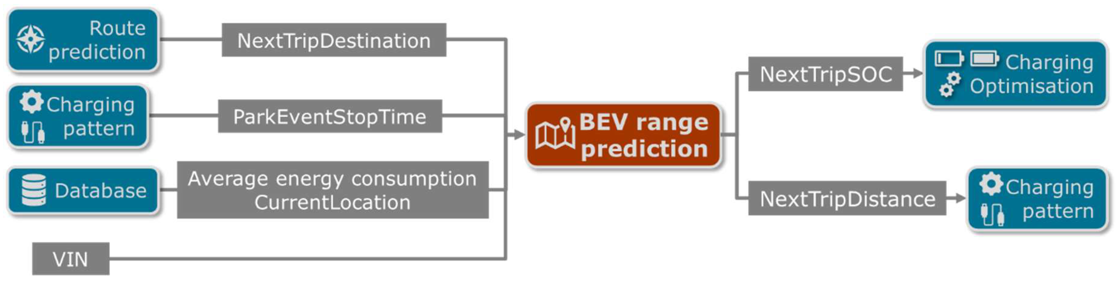
3.3. BEV Range Prediction

The purpose of this algorithm is to predict the range required for the next trip; it requires knowledge of the next trip distance. The next trip SOC is then input into the charging optimisation, while the next trip distance is an input for the second part of the charging pattern (Figure 9).

The BEV range prediction is a well-known research topic in order to accurately define the BEV range and reduce the range of anxiety [42,43]. The fundamental input is historical data. Additionally, road type, driving style or weather could be taken into account for the improvement in prediction accuracy. A previous study [44] created three models: physical, energy and SOC-based. For the current study, only an energy-based model is implemented. Different models have been developed considering distance, road type and average vehicle speed with the purpose of predicting the next trip average consumption. The first model considering the overall consumption is predicting only one single average consumption value, which is not accurate enough. The second and third models consider, respectively, the next trip distance and the next trip road type. Unlike the first method, these methods provide more accurate results, but the prediction is slightly underestimated. A fourth model considers the road type and the average vehicle speed but does not improve the results. Finally, the fifth method, using average fuel consumption and average vehicle speed, provides the most accurate prediction. A post-processing step is necessary to calculate the average consumption versus average vehicle speed trendline. This trendline is stored in the database (Figure 10) and will be updated regularly to consider the latest data. Figure 10 depicts the trendline using all vehicles’ data; however, for better optimisation, each vehicle has its own trendline made with its own data. For each trip, the consumption and speed are averaged and displayed. From the figure shown, a trend can be seen with high average consumption for average speed lower than 10 km/h. Then, from 10 km/h to 50 km/h, average consumption remains almost constant. Finally, above 50 km/h, the average consumption increases as the average speed. The average blue line is defined as calculating the average of average consumption for each time window of 1 km/h.

With knowledge of the next trip destination, start time and location, the next trip distance and average speed are defined using Google API (Figure 11). Next trip average speed combined with the trendline stored in the database allows getting the next trip average consumption. The rest of the calculation follows from the following equations:

$$E_{NextTrip}\left[\mathrm{kWh}\right]=Consumptio{n}_{NextTrip}\times Distanc{e}_{NextTrip}$$

(6)

$$SO{C}_{NextTrip}[\%]=\frac{E_{NextTrip}}{C_{Battery}}\times 100$$

(7)

Each vehicle has its own trendline defined using its own data; therefore, an assumption of having one unique driver per vehicle is made, and the average consumption is tailored for each vehicle. This is a way to consider somehow the driving style, as an aggressive driving style leads to higher consumption as compared to a calm driving style.

3.4. Charging Optimisation

The last algorithm is fundamental, where the charging power profile is defined. The inputs are the initial SOC, the SOC for the next trip, the parking duration (start and stop date-time), charger power and electricity cost. All these parameters allow the charging optimisation to define the power profile with duration, cost, power and SOC constraints (Figure 12).

Charging optimisation topics have been studied in previous projects. Some studies utilise Dynamic Programming (DP) [45,46], Multi-Objective Particle Swarm Optimisation (MOPSO) [47], Genetic Algorithm (GA) [48] or heuristic method [49] to define an optimal way to define the charging profile considering different parameters: charging duration, efficiency, charging voltage, temperature, grid operation cost, etc.

The charging optimisation utilises DP as it allows the computation of the global optimal solution. DP has been widely used for path optimisation and to obtain an optimal SOC profile of hybrid electric vehicles [50]. In this project, DP will be used to find the optimal charging power profile. The principle of DP is to break down a complicated problem into multiple and simpler problems to solve. First, DP runs backwards from the end of the optimisation problem to the beginning to construct a map of optimal control actions at all possible state variable values and time steps. From this, the related optimal state variable profile can be obtained by simply simulating the model forward in time. Starting from a known initial state and proceeding towards the end of the problem, a one-time step at a time while determining the optimal control action at each time step based on the optimal control map. Optimality is defined with respect to the cost function (8) that is made of two parts: the electricity cost when charging or discharging and the battery degradation cost. Each of the parts is in units of GBP and have a weighting factor. The optimal solution must additionally respect the problem constraints, such as the final SOC (originating from BEV range prediction, NextTripSOC) level that will allow covering the next trip distance. The state variable chosen for this optimisation problem is the battery SOC, whereas the charger power acts as the control variable. Here, the power to charge or discharge the battery will be capped between the minimum and maximum charger power. It is assumed that all chargers are reversible, hence allowing V2G usage. The last parameter to be defined is the grid discretisation of the state and control variables (battery SOC and charging power, respectively), as well as the length of the time step. Generally, the finer the discretisation size, the more accurately the discretised optimisation problem approximates the underlying continuous problem. Thus, the optimal solution obtained from the discretised problem is closer to the optimal solution of the real-world continuous problem. On the other hand, a finer discretisation grid will increase the number of computations required and will consequently take longer to complete. The discretisation is fixed in order to spend around 1% of the charging event duration to compute DP.

$$J=w_{1}cos{t}_{chg/dchg}+w_{2}cos{t}_{batt degradation}$$

(8)

$$cos{t}_{chg/dchg}\left[GBP\right]=P_{chg/dchg}cos{t}_{elec}$$

(9)

$$cos{t}_{batt degradation}\left[GBP\right]={\Delta }_{bat}\left(t\right).cos{t}_{batt}$$

(10)

where $cos{t}_{chg/dchg}$ (9) is the electricity cost when charging or discharging the battery, where $P_{chg/dchg}$ the power when charging and discharging in kWh, and $cos{t}_{elec}$ the electricity cost in GBP/kWh. The parameter $cos{t}_{batt degradation}$ (10) comes from the battery model where the degradation is evaluated in GBP. Where ${\Delta }_{bat}\left(t\right)$ is the battery degradation in Ah, and $cos{t}_{batt}$ is the battery cost in GBP/Ah. Each of these two parameters has their unitless weighting factor: $w_1$ for the electricity cost, and $w_2$ for the battery degradation. The modelling is based on a previous study [51].

$${\Delta }_{bat}\left(t\right)=\frac{1}{Q_{bat-max}}{{\displaystyle \int }}_0^t\left|F\left(So{C}_{bat}\right)G\left(i_{bat}\right)i_{bat}\left(t\right)\right|dt,$$

(11)

$$F\left(So{C}_{bat}\right)=1+3.25{\left(1-So{C}_{bat}\right)}^2,$$

(12)

$$\{\begin{array}{c}G\left(i_{bat}\right)=1+0.45\frac{i_{bat}}{i_{bat-nom}}if i_{bat}\ge 0\\ \\ G\left(i_{bat}\right)=1+0.55\frac{\left|i_{bat}\right|}{i_{bat-nom}}if i_{bat}<0\end{array},$$

(13)

where $Q_{bat-max}$ is the entire life battery capacity, $So{C}_{bat}$ is the battery SOC, $i_{bat}$ is the battery current, and $i_{bat-nom}$ is the nominal battery current.

While minimising the cost function, the DP solution must also respect boundary conditions. The final battery SOC ($SO{C}_{bat, final}$) must be greater than or equal to the SOC required to complete the next trip (14). The SOC must stay between the minimum and maximum operational limits ($SO{C}_{bat, min}$, $SO{C}_{bat, max}$, (15)). The charger power that restricts the SOC rate of change must be limited between the minimum and maximum charger power ($P_{charger,min}$,$P_{charger,max}$, (16)).

$$SO{C}_{bat,final}\ge SO{C}_{NextTrip}$$

(14)

$$SO{C}_{bat,min}\le SO{C}_{bat}\le SO{C}_{bat,max}$$

(15)

$$P_{charger,min}\le P_{charger}\le P_{charger,max}$$

(16)

The optimal charging power profile is generated and then sent to the vehicle onboard charger controller (Figure 13). The benefits of the DP optimisation have been discussed later in this paper. The DP algorithm has been tested in multiple scenarios where charging duration is 1 h, starting SOC is 30%, and the final SOC target is 40%. The varying parameter is the electricity cost when buying or selling.

Table 6. DP (Dynamic Programming) algorithm tested for multiple scenarios.

Scenario	Tariff Name	Electricity Cost				Balance
		Buying		Selling
		Rate 1	Rate 2	Rate 1	Rate 2
		(GBP/kWh)	(GBP/kWh)	(GBP/kWh)	(GBP/kWh)	(GBP)
1	Standard	0.162	0	0	0	−0.39
2	Eco7	0.197	0.088	0	0	−0.21
3	Standard + V2G1	0.162	0	0.4	0	0.11
4	Eco7 + V2G1	0.197	0.088	0.4	0	0.45
5	Eco7 + V2G2	0.197	0.088	0.45	0.25	0.55

shows the experimental results of the DP algorithm. The electricity costs have been explained in Section 2, and they are linked to tariff names in the table. “Standard” refers to the one-rate tariff when buying. “Eco7” is the two-rate tariff when buying. “V2G₁” is the one-rate tariff when selling. “V2G₂” is the two-rate tariff when selling. The “Balance” column is the sum of the electricity bought with the electricity sold. When the balance is negative, the BEV owner spends money during the charging event and earns money if the balance is positive. Scenario 1 without V2G can be compared with scenario 3 with V2G. A benefit of GBP 0.5 is observed in this specific case when V2G is used. 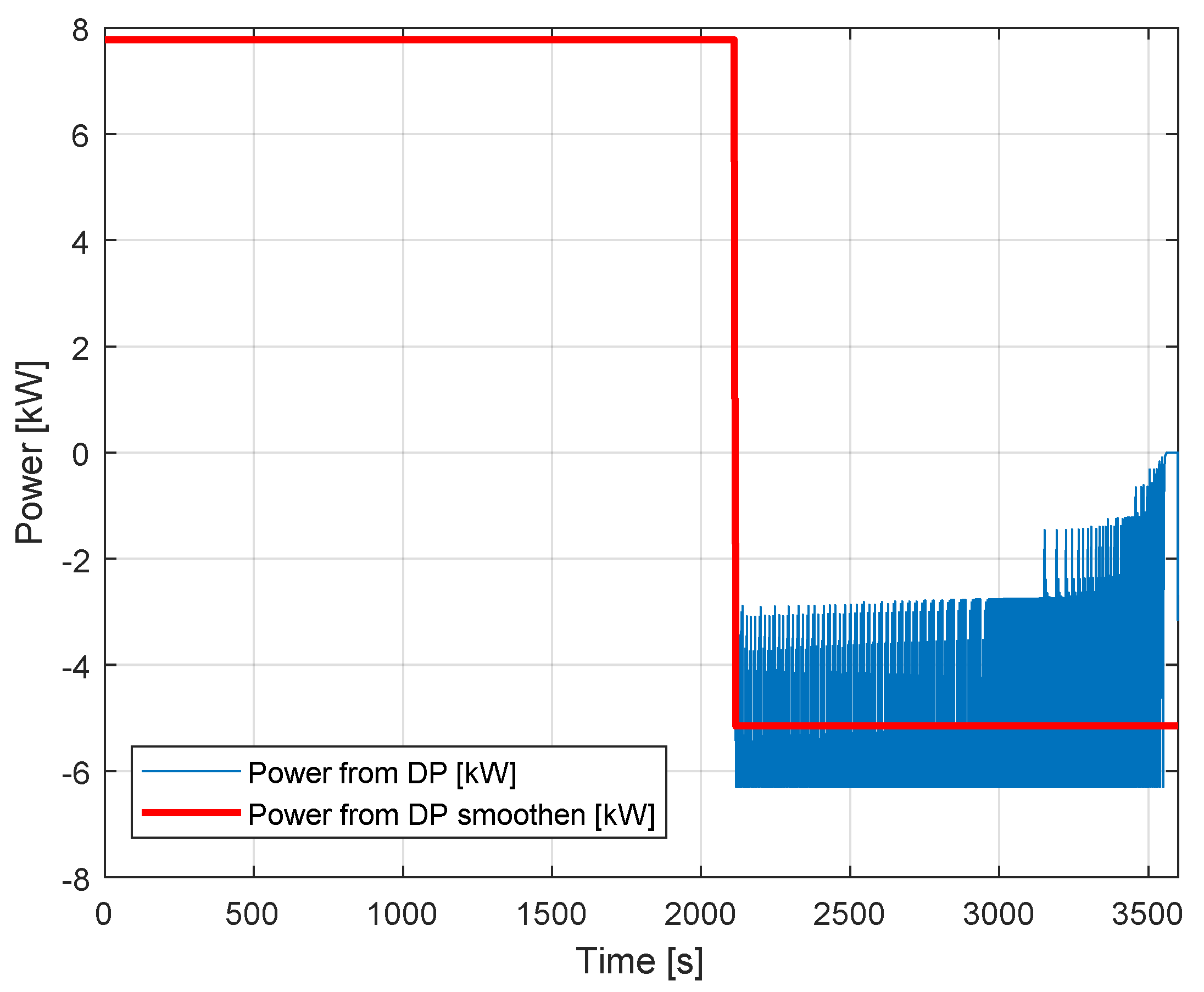Similarly, the comparison of scenario 2 and 5 (Figure 13, Figure 14) shows that the BEV owner can make up to GBP 0.76 benefits with V2G tariffs. Assuming this scenario can happen between 1 h to 5 h per day during a year, the annual benefits can range from GBP 200 to GBP 1400.

Figure 14 shows the optimal charging profile for scenario 5. Two traces are visible—the raw power profile in blue and the smoothen power profile in red. The raw power profile contains many oscillations, especially when the power is negative. This is due to a numerical error related to DP calculation. These oscillations are not acceptable for both the electrical grid and the BEV, that is why the power profile needs to be filtered. The raw power profile is averaged during the oscillation events while keeping the same optimisation results.

3.5. Dashboard

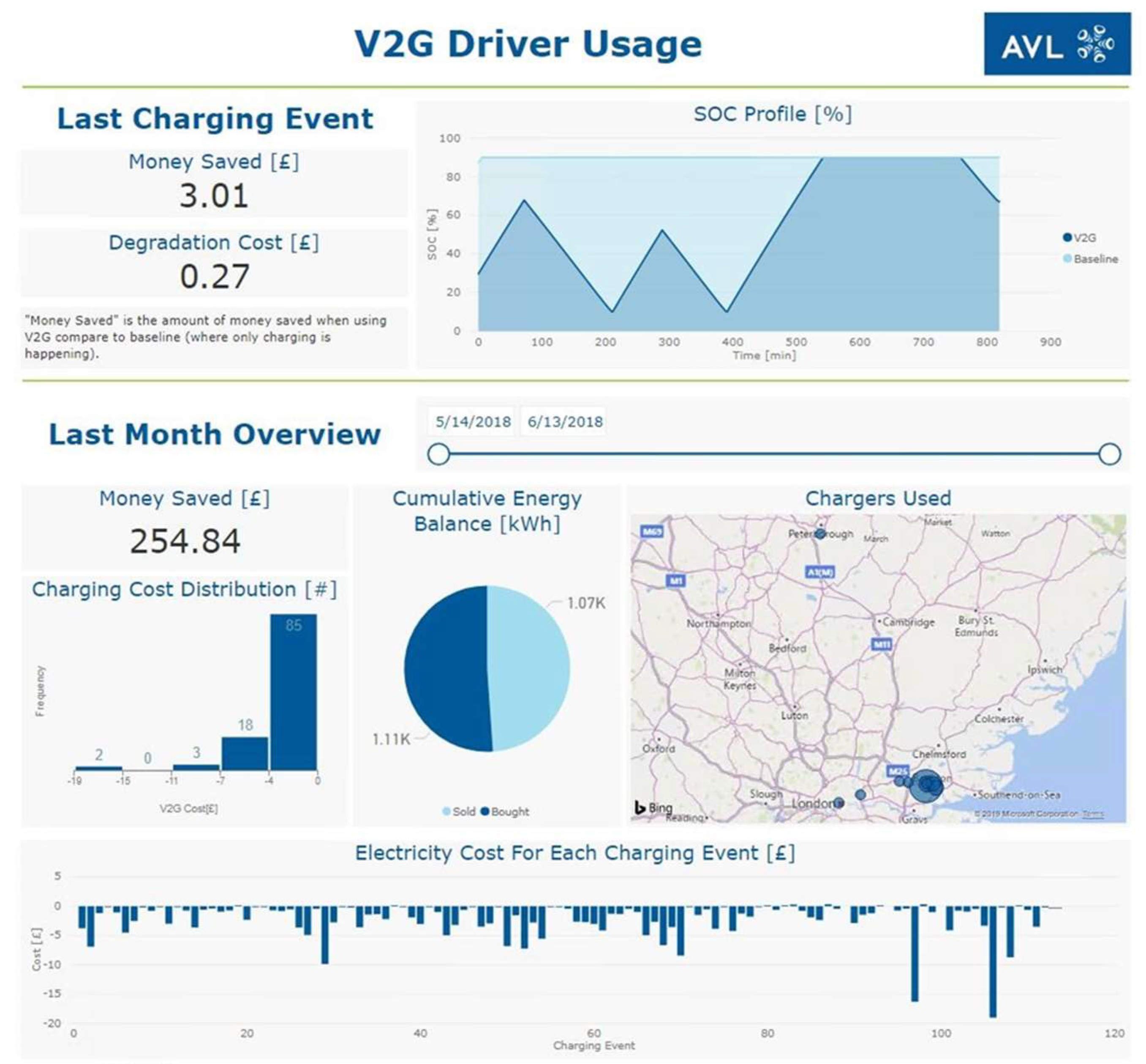
The dashboards are key to communicate the optimisation results to the target customers. BEV owners can track the amount of money their BEVs have earned when selling energy to the grid (Figure 15). OEMs can understand how the battery behaves under V2G use and how the battery could be improved in terms of performance, for example. Finally, utility companies and charger providers can analyse and understand the energy flow associated with V2G and plan for further infrastructure investments.

4. Discussion

The assumptions on the previous part emphasise a financial benefit for the vehicle owner when using V2G. The goal here is to confirm these assumptions using real-world data. One month of real-world data has been aggregated to evaluate the benefits. Three cases have been studied: Case 1: V2G with DP, Case 2: no V2G with DP and Case 3: no V2G without DP. Case 1 allows the BEV owner to sell electricity to the grid and benefit from a charging/discharging optimisation, thanks to DP. Case 2 considers only charging optimisation with DP. Case 3 acts as a basic charging feature, the battery is charged at full charger power available until either the SOC is maximum or until the end of the charging event.

As the data used are logged from conventional vehicles, it may occur that the trip distance is too great or charging event too short for the BEV battery range. These few cases are considered and compensated in the final cost column (

Table 7. Charging cost comparison for different charging system cases.

Case	V2G	DP	One-Month Total Cost (GBP)
Case 1	Yes	Yes	−137
Case 2	No	Yes	14
Case 3	No	No	20

). The cost column summarises the amount spent (positive) or earnt (negative), and it already considers the battery degradation cost. Case 3 is the costliest for the driver as there is no possibility to sell electricity to the grid. Furthermore, the charging takes place at full power without considering the possibility of waiting for a lower electricity tariff. Adding the optimisation, thanks to DP, the driver can benefit from cheaper electricity cost to reduce the charging cost of case 2. Case 1 makes the driver earning money while making its battery available for grid support. Despite the important financial benefits, the battery degrades faster.

The battery lifetime decreases due to the extended usage, which leads to a reduction of the battery performance. The degradation weighting factor, from DP cost function, must be increased to preserve the battery. The same month of data, run previously in simulation, is run again with higher values of the degradation weighting factor, ranging from 1 to 10,000. According to Han [52], battery life can be evaluated using Depth-of-Discharge (DOD) with 80% as a lifetime target. This statement coincides with the OEMs warranty in terms of battery performance. Based on the initial battery cost (GBP 3720, assuming 200 US $/kWh from [51] and US $ 1.29 ≈ GBP 1), the battery minimum value limit is GBP 2978 to ensure good performance, assuming linear degradation. A degradation weighting factor set to a value of 1 gives a lifetime of around 1 year; the BEV owner will obtain high financial benefits, around GBP 2800 for the first year, but the battery will need to be replaced much earlier than in the case of conventional battery usage. This financial benefit for the first year is based on one-month simulation with a bit more than 600 km driven in about 18 h, and about 700 h spent on charging/discharging. Increasing the degradation weighting factor acts as a deterrent to selling electricity to the grid, decreasing in the process the revenue from selling electricity to the grid; therefore, the degradation cost decreases, and the life of the battery is extended (Figure 16). A weighting factor values trade-off must be defined between the immediate cost benefits and the battery degradation according to the customer’s needs. An exponential trendline is drawn to model the trade-off between battery degradation and electricity cost based on the simulation points. For this user and with the assumed electricity cost, the optimal point is calculated. This point is where the sum of electricity sold (GBP-270) and the battery degradation cost (GBP 115) are maximised. It allows this user to gain GBP 155 for one month, with a degradation weighting factor value lower than 1.

This solution and its associated benefits rely on the BEV owner’s willingness to share their data and participate in V2G. Without this participation, the solution developed cannot be optimum or even not useable for BEV owners that do not share their data. For people having concern about data privacy and those who do not want to be tracked, another solution must be developed.

5. Conclusions

This work demonstrates the potential financial benefits of V2G for the BEV owners by using their battery as an energy buffer. The financial benefit is estimated at around GBP 2800 for the first year considering the simplifying assumptions taken. This can be achieved by smart data usage enabled by the cloud-based big data platform. The data structure provides rapid and uncomplicated access to the necessary data for the prediction algorithm, which is based on machine learning techniques. The prediction results are then aggregated to feed dashboards, providing essential information to the target customers.

Despite financial benefits for the BEV owners, V2G implementation increases battery usage cycles and thus leads to quicker battery degradation. Therefore, OEMs must consider the early degradation of batteries when designing next-generation batteries for V2G-capable vehicles. Regarding the electricity cost when selling to the grid, a trade-off must be found to satisfy both the vehicle owners and the utility company.

As a next step, real-world data from BEV must be employed to attain more accurate results. In addition, real-world testing could be performed to demonstrate the capability of these algorithms and allowing further improvement in the process. The charging optimisation detailed in this paper does not consider the grid, which could be critical during grid peak demands. The grid loads are not considered and could be added to the cost function (8) as a third parameter. With high BEV penetration, start charging at the same time or during peak time, when millions of BEVs could overwhelm the grid. Also, a solution to make sure BEVs do not charge at the same time, leading to new peak demand, must be developed. Approaches considering the grid load have been studied in past projects, where a penalty parameter is used [53]. On top of the grid load consideration, renewable energies integration could be added to the grid ecosystem. The portion of renewable energies generation in the electricity mix increases; however, the renewable energy generation fluctuates due to weather conditions. Then, BEV could be charged more when renewable generation is high and then discharged more when grid load is high. Hence, optimisation could be achieved, taking into account BEV needs, grid load and renewables. Furthermore, additional data, such as traffic information, could be used to improve further the prediction accuracy. Finally, the security of the V2G transactions could be improved using technology, such as blockchain, based on previous work [54,55,56].