Comparison of the Economic and Environmental Performance of V2H and Residential Stationary Battery: Development of a Multi-Objective Optimization Method for Homes of EV Owners

Abstract
:1. Introduction
2. Method
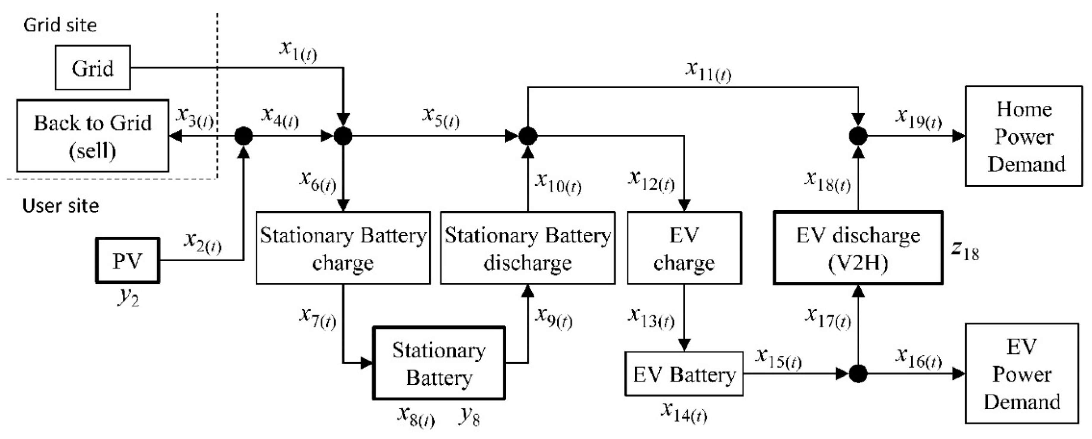
2.1. Modeling
- To obtain min{fcost(x1, x3, y2, y8, z18)} in Equation (1), the problem takes the following form:min. objective function Equation (2)
subject to: optimization constraints Equations (7) to (28) - To obtain min{fco2(x1)} in Equation (1), the problem takes the following form:min. objective function Equation (3)
subject to: optimization constraints Equations (7) to (28) - Substitute min{fcost(x1, x3, y2, y8, z18)} and min{fco2(x1)} calculated in the previous two steps into Equation (1) to solve the problem described as following form:min. objective function Equation (1)
subject to: optimization constraints Equations (7) to (28)
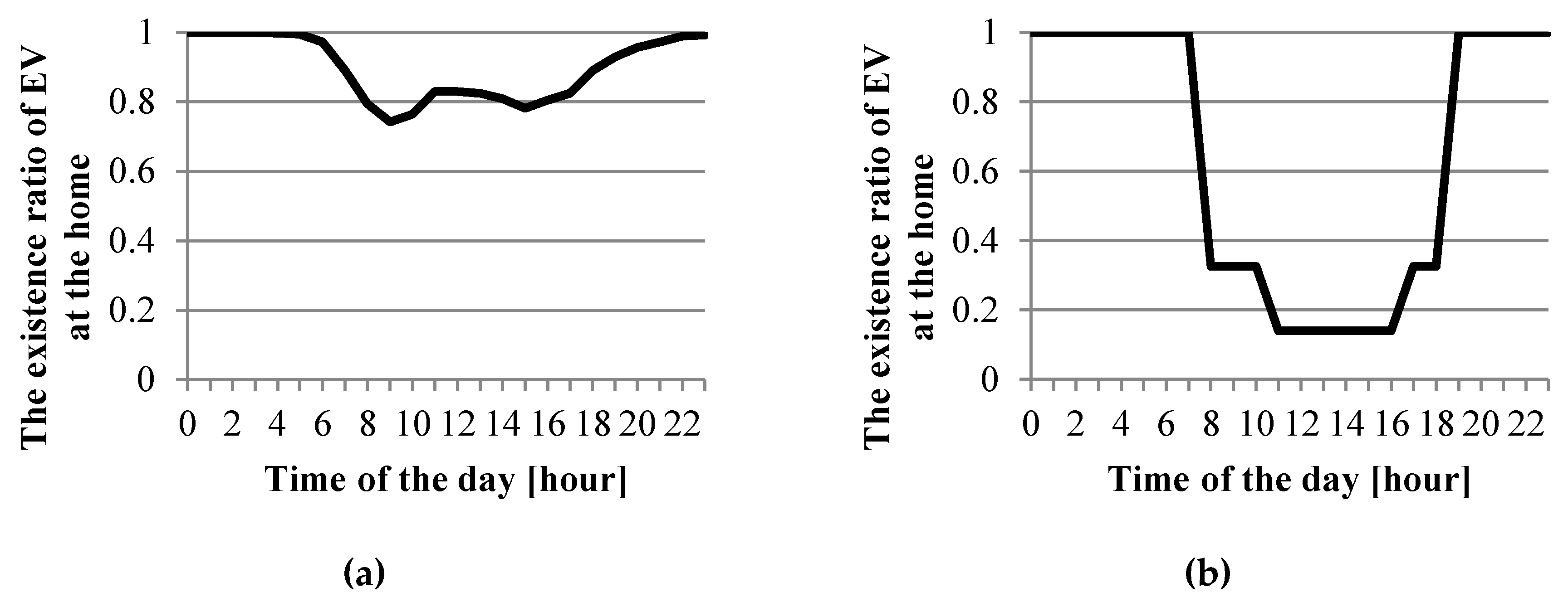
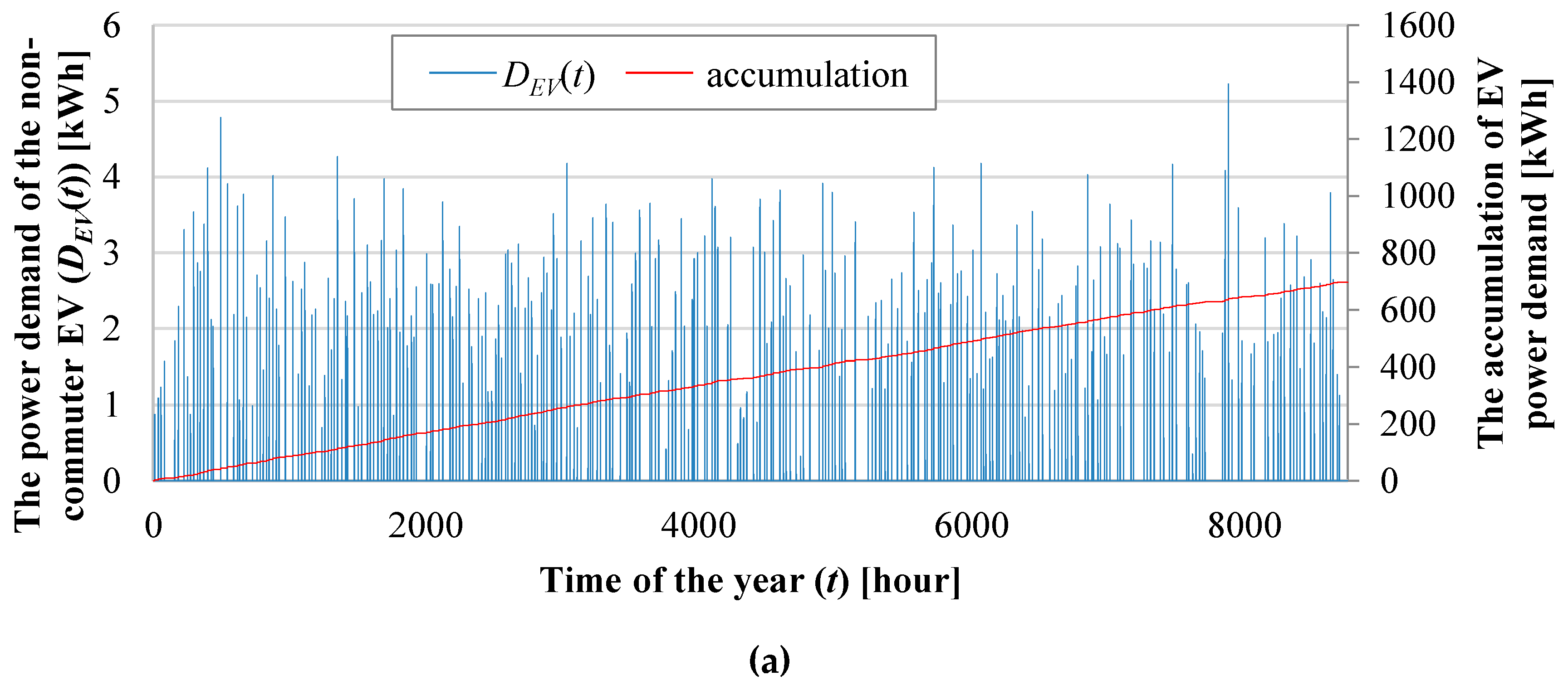
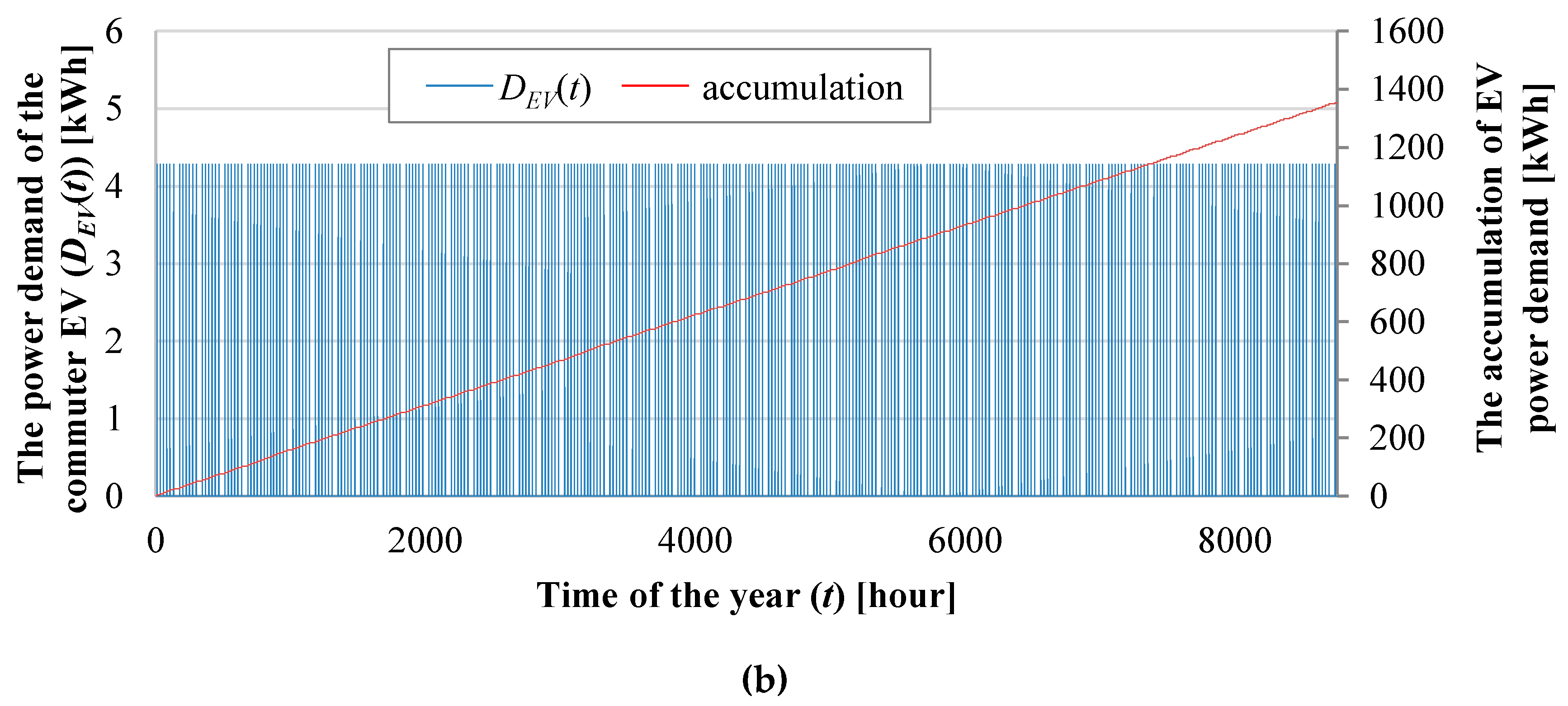
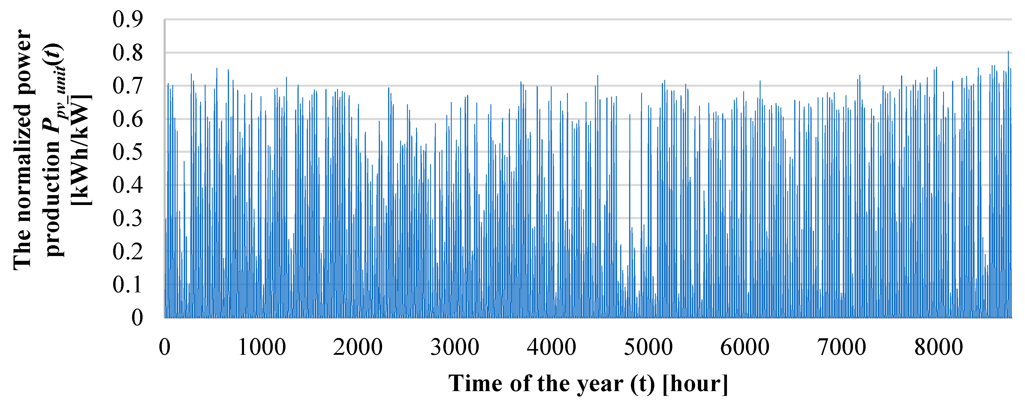
2.2. Sample System
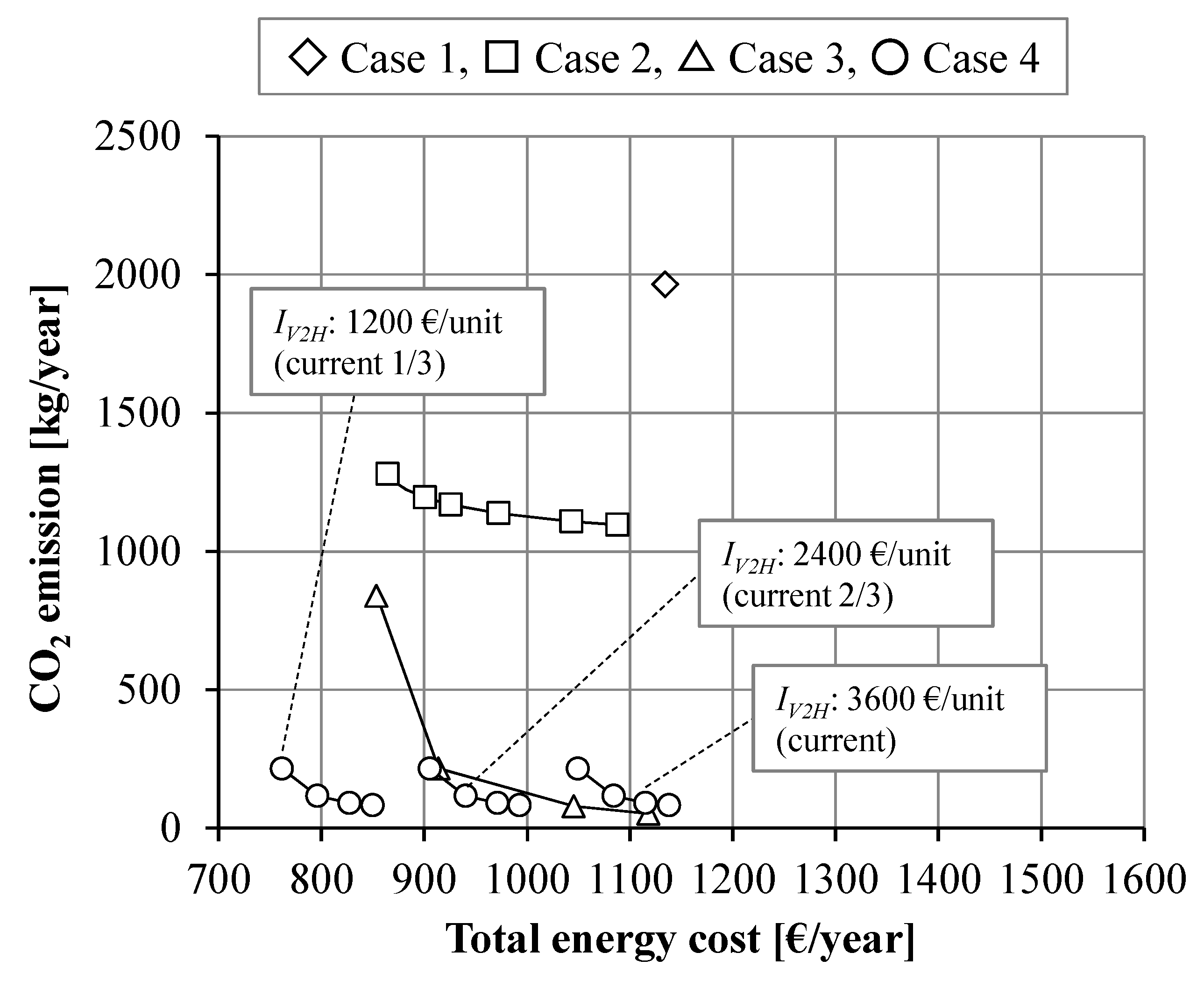
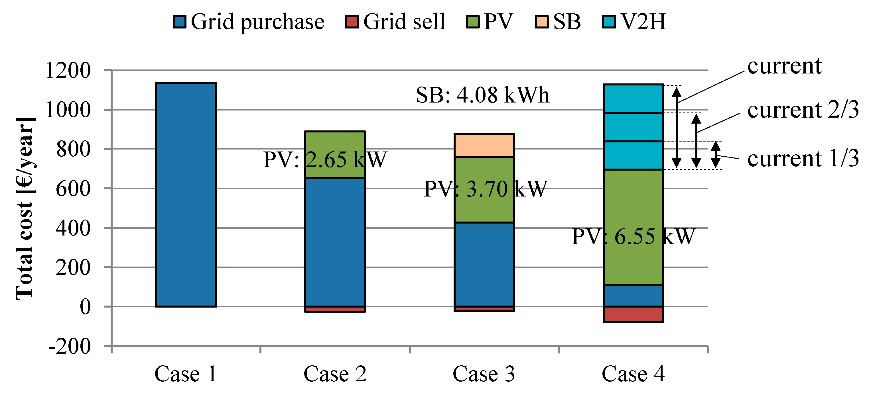
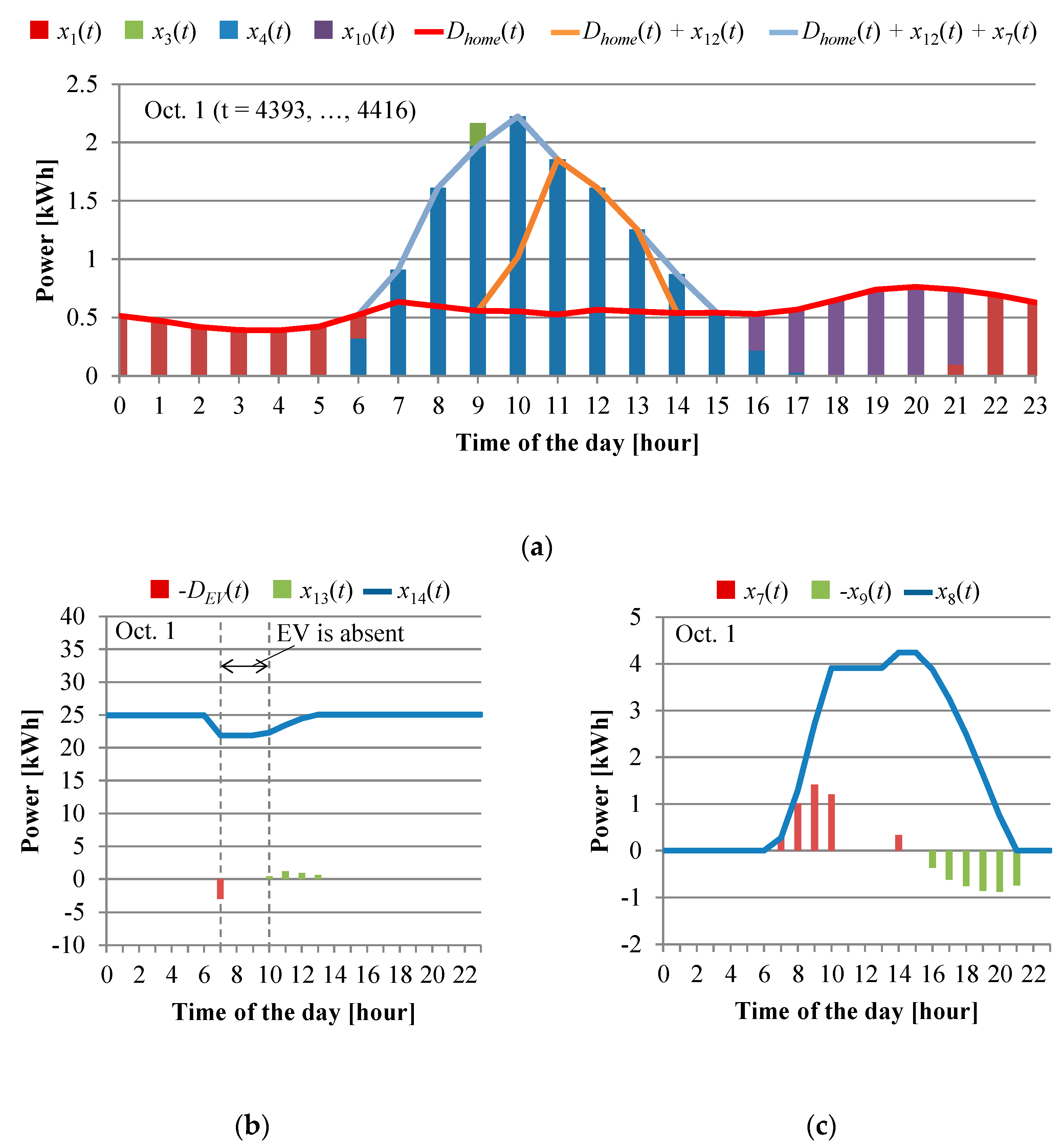
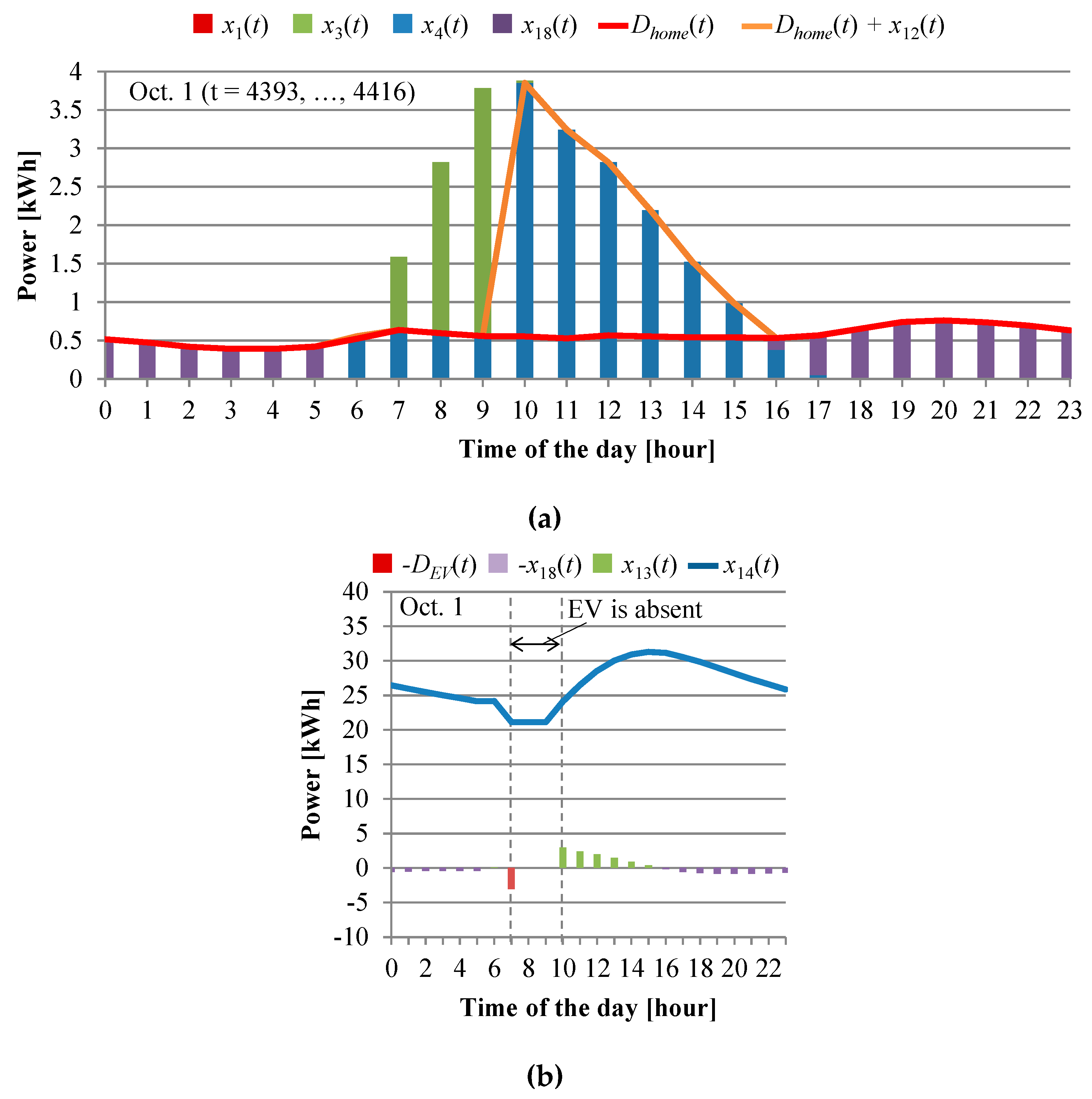
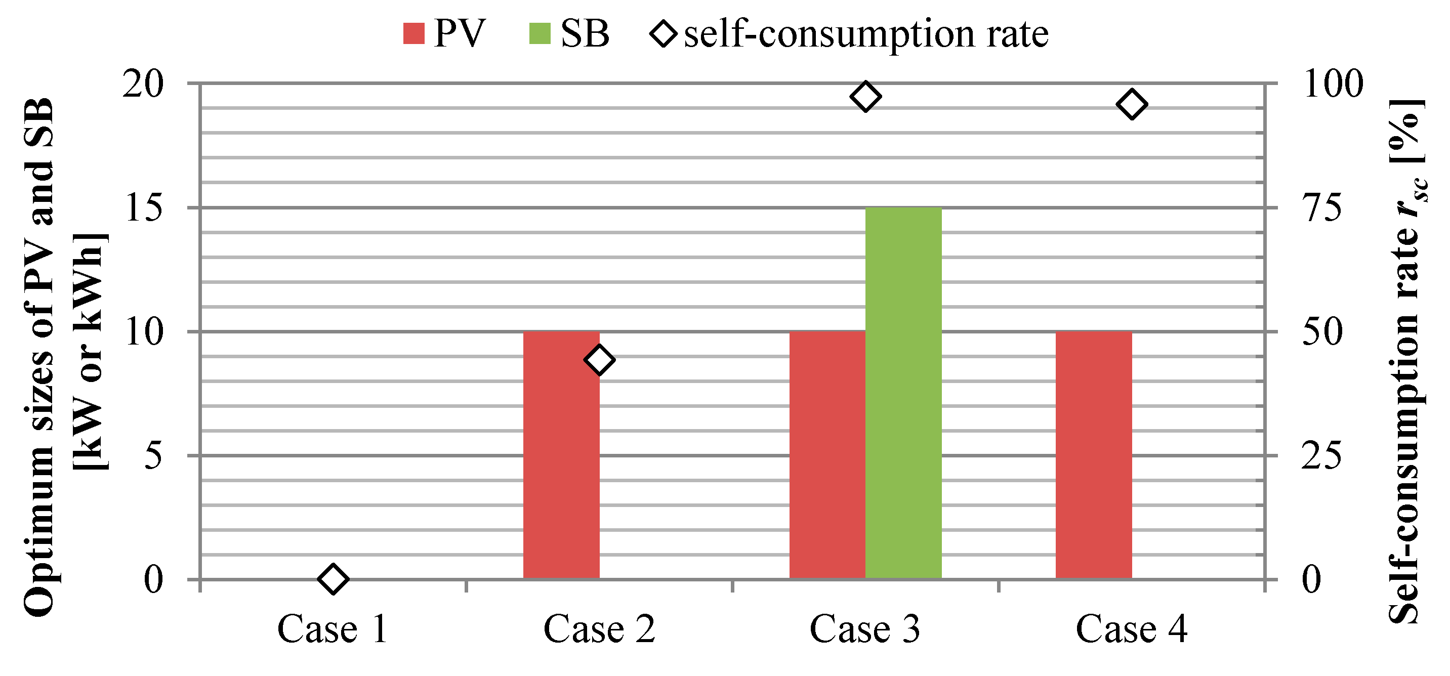
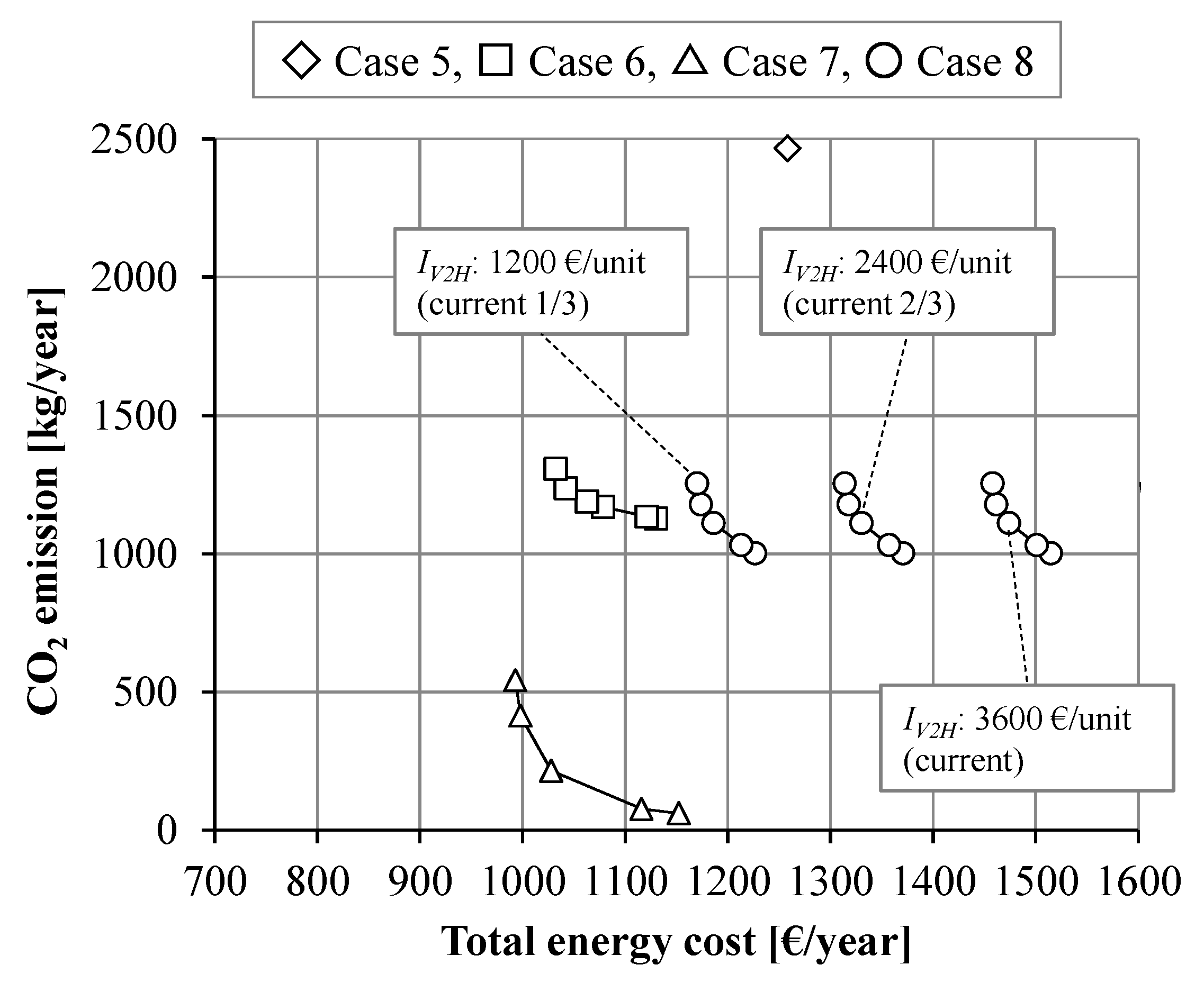
3. Results
4. Discussion
5. Conclusions
Author Contributions
Funding
Conflicts of Interest
Nomenclature
| Set | |
| t | index of optimization periods, t = 1, 2, ..., T (hour) |
| Variables | |
| xi(t) (i = 1, ..., 19) | energy flow or state of charge in period t (kWh) |
| y2 | size of PV (kW) |
| y8 | size of SB (kWh) |
| z18 | necessity of V2H system (binary variable) (unit) |
| fcost | total energy cost (€) |
| fCO2 | total CO2 emission (kg-CO2) |
| Parameters | |
| T | time horizon of the optimization problem (hour) |
| pbuy(t) | purchase unit price in period t (€/kWh) |
| psell(t) | selling unit price in period t (€/kWh) |
| CPV | cost coefficients of PV (€/kW/hour) |
| CSB | cost coefficients of SB (€/kWh/hour) |
| CV2H | cost coefficients of V2H (€/unit/hour) |
| IPV | investment cost of PV (€/kW) |
| ISB | investment cost of SB (€/kWh) |
| IV2H | investment cost of V2H (€/unit) |
| MPV | annual maintenance cost of PV (€/kW/year) |
| MSB | annual maintenance cost of SB (€/kWh/year) |
| MV2H | annual maintenance cost of V2H (€/unit/year) |
| LPV | product life of PV (year) |
| LSB | product life of SB (year) |
| LV2H | product life of V2H (year) |
| egrid | CO2 emission rate for grid power (kg-CO2/kWh) |
| PPV_unit(t) | normalized power production of PV in period t (kWh/kW) |
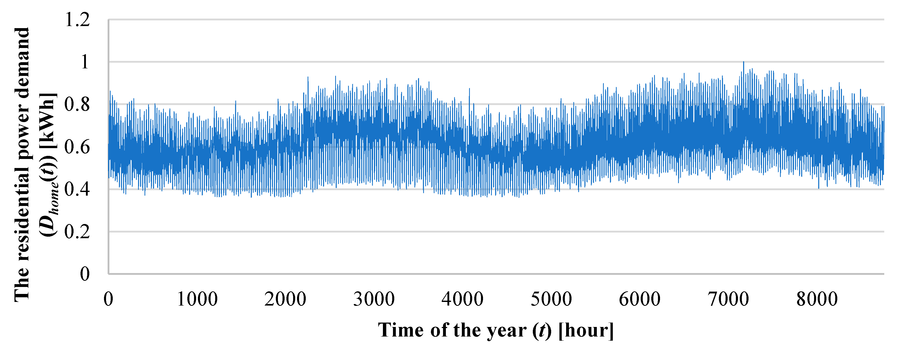
| DEV(t) | power demand to drive EV in period t (kWh) |
| Dhome(t) | residential power demand in period t (kWh) |
| Cap.EV | capacity of EV battery (kWh) |
| rEV_ini. | ratio of initial SoC |
| lbEV_SOC | lower limit of SoC (kWh) |
| ubEV_SOC | upper limit of SoC (kWh) |
| PVmax | maximum size of PV (kW) |
| SBmax | maximum size of SB (kW) |
| ηSB_Ch. | efficiency of charging for SB |
| ηSB_DisCh. | efficiency of discharging for SB |
| rSB_ini. | ratio of initial SoC for SB |
| rSB_Ch. | ratio of charging power for SB |
| rSB_DisCh. | ratio of discharging power for SB |
| ηEV_Ch. | efficiency of charging for EV |
| ηEV_DisCh. | efficiency of discharging for EV |
| PEV_Ch. | charging power for EV (kW) |
| PEV_DisCh. | discharging power for EV (kW) |
| δEV (t) | the absence of the EV in period t |
| DT | departure time (hour) |
| CT | comeback time (hour) |
| ST | stay time (min) |
| DP | driving period (min) |
| TL | trip length (km) |
| V | average driving speed of EV (km/h) |
| w | weight of objectives |
Appendix A
- LCOE = the levelized cost of electricity;
- Ii = investment expenditures in the year i;
- Mi = operations and maintenance expenditures in the year i;
- Fi = fuel expenditures in the year i;
- Ei = electricity generation in the year i;r = discount rate; and
- n = life of the system.
References
- Ministry of Economy, Trade and Industry. The 5th Strategic Energy Plan; METI: Tokyo, Japan, 2018. Available online: https://www.enecho.meti.go.jp/en/category/others/basic_plan/5th/pdf/strategic_energy_plan.pdf (accessed on 1 October 2019).
- Kaschub, T.; Jochem, P.; Fichtner, W. Interdependencies of Home Energy Storage between Electric and Stationary Battery. World Electr. Veh. J. 2013, 6, 1144–1150. [Google Scholar] [CrossRef]
- Erdinc, O.; Paterakis, N.G.; Mendes, T.D.P.; Bakirtzis, A.G.; Catalao, J.P.S. Smart Household Operation Considering Bi-directional EV and ESS Utilization by Real-Time Pricing-Based DR. IEEE Trans. Smart Grid 2015, 6, 1281–1291. [Google Scholar] [CrossRef]
- Wu, X.; Hu, X.; Moura, S.; Yin, X.; Pickert, V. Stochastic control of smart home energy management with plug-in electric vehicle battery energy storage and photovoltaic array. J. Power Sources 2016, 333, 203–212. [Google Scholar] [CrossRef]
- Erdinc, O.; Paterakis, N.G.; Pappi, I.N.; Bakirtzis, A.G.; Catalao, J.P.S. A new perspective for sizing of distributed generation and energy storage for smart households under demand response. Appl. Energy 2015, 143, 26–37. [Google Scholar] [CrossRef]
- Wu, X.; Hu, X.; Teng, Y.; Qian, S.; Cheng, R. Optimal integration of a hybrid solar-battery power source into smart home nanogrid with plug-in electric vehicle. J. Power Sources 2017, 363, 277–283. [Google Scholar] [CrossRef]
- Naghibi, B.; Masoum, M.A.S.; Deilami, S. Effects of V2H Integration on Optimal Sizing of Renewable Resources in Smart Home Based on Monte Carlo Simulations. IEEE Power Energy Technol. Syst. J. 2018, 5, 73–84. [Google Scholar] [CrossRef]
- Technology Collaboration Programme on Hybrid and Electric Vehicles (HEV TCP). Hybrid and Electric Vehicles -The Electric Drive Hauls-; International Energy Agency: Paris, France, 2019; pp. 67–73. Available online: http://www.ieahev.org/assets/1/7/Report2019_WEB_New_(1).pdf (accessed on 1 October 2019).
- Zakariazadeh, A.; Jadid, S.; Siano, P. Multi-objective scheduling of electric vehicles in smart distribution system. Energy Convers. Manag. 2014, 79, 43–53. [Google Scholar] [CrossRef]
- Kataoka, R.; Shichi, A.; Yamada, H.; Iwafune, Y.; Ogimoto, K. Evaluation of Economic and Environmental Superiority of EV Battery in Power Systems: Development of Multi-objective Optimized Model for V2H. In Proceedings of the 32nd Electric Vehicle Symposium (EVS32), Lyon, France, 19–22 May 2019. [Google Scholar]
- MathWorks, Optimization Toolbox. Available online: https://jp.mathworks.com/help/optim/index.html?lang=en (accessed on 1 October 2019).
- Mustapha, A.; Fonseca, J.G.D.S., Jr.; Oozeki, T.; Iwafune, Y. Evaluation of Residential PV-EV System for Supply and Demand Balance of Power System. IEEJ Trans. Power Energy 2015, 135, 27–34. (In Japanese) [Google Scholar] [CrossRef]
- Iwafune, Y.; Ogimoto, K.; Azuma, H. Integration of Electric Vehicles into the Electric Power System Based on Results of Road Traffic Census. Energies 2019, 12, 1849. [Google Scholar] [CrossRef]
- The Energy Conservation Center, Japan. Results of the Survey of Standby Power Consumption. 2013. (In Japanese) [Google Scholar]
- Morita, K.; Manabe, Y.; Kato, T.; Funabashi, T.; Suzuoki, Y. An Evaluation of Average Electricity Demand Characteristics with Hundreds of Households. J. Jpn. Soc. Energy Resour. 2016, 38, 20–29. (In Japanese) [Google Scholar] [CrossRef]
- New Energy and Industrial Technology Development Organization, MEteorological Test data for PhotoVoltaic System. Available online: http://www.nedo.go.jp/library/nissharyou.html (accessed on 1 October 2019).
- Power Generation Cost Analysis Working Group, Report on Analysis of Generation Costs, Etc. for Subcommittee on Long-term Energy Supply- demand Outlook. 2015. Available online: https://www.meti.go.jp/english/press/2015/pdf/0716_01b.pdf (accessed on 1 October 2019).
- Kobashi, T.; Say, K.; Wang, J.; Yarime, M. Techno-economic analyses of PV, PV + battery, PV + EV for household in Kyoto and Shenzhen towards 2030. In Proceedings of the 35th Energy Systems Economic Environment Conference, Tokyo, Japan, 30 January 2019; pp. 383–386. (In Japanese). [Google Scholar]
- Ministry of Economy, Trade and Industry. Available online: http://www.meti.go.jp/committee/kenkyukai/energy_environment/energy_resource/pdf/ 005_08_00.pdf (accessed on 1 October 2019).
- Mitsubishi Research Institute, Inc. 2017. Available online: https://www.meti.go.jp/meti_lib/report/H28FY/000479.pdf (accessed on 1 October 2019).
- Nichicon Corp., EV Power Station. Available online: https://www.nichicon.co.jp/products/v2h/about/ (accessed on 1 October 2019).
- Chubu Electric Power Co. Inc. Available online: http://www.chuden.co.jp/home/home_menu/home_basic/otoku/index.html (accessed on 1 October 2019).
- The Federation of Electric Power Companies of Japan, Expanding Use of Non-Fossil Energy Sources. Available online: https://www.fepc.or.jp/english/environment/global_warming/nuclear_lng/ (accessed on 1 October 2019).
- Hara, T. Technology Assessment based on Range Analysis of the Linear-Programming Bottom-up Energy Systems Model. J. Jpn. Soc. Energy Resour. 2019, 40, 202–219. (In Japanese) [Google Scholar] [CrossRef]
- International Renewable Energy Agency; Data Methodology. 2015. Available online: http://dashboard.irena.org/download/Methodology.pdf (accessed on 1 October 2019).
- Landi, M. Vehicle-to-Grid developments in the UK. In Proceedings of the 32nd Electric Vehicle Symposium (EVS32), Lyon, France, 19–22 May 2019. [Google Scholar]


| Case | EV Driving Pattern | System Configurations | |||
|---|---|---|---|---|---|
| Grid | PV | SB | V2H | ||
| 1 | Non-commuter | ○ | - | - | - |
| 2 | ○ | ○ | - | - | |
| 3 | ○ | ○ | ○ | - | |
| 4 | ○ | ○ | - | ○ | |
| 5 | Commuter | ○ | - | - | - |
| 6 | ○ | ○ | - | - | |
| 7 | ○ | ○ | ○ | - | |
| 8 | ○ | ○ | - | ○ | |
| Vehicle efficiency | 7 | (km/kWh) | |
| Capacity of EV battery | (Cap.EV) | 40 | (kWh) |
| Ratio of initial SoC | (rEV_ini.) | 0.5 | |
| Lower limit of SoC | (lbEV_SOC) | 8 | (kWh) |
| Upper limit of SoC | (ubEV_SOC) | 32 | (kWh) |
| Equipment | Parameter | |||
|---|---|---|---|---|
| PV | Investment cost | (IPV) | 2064 | (€/kW) |
| Maintenance cost | (MPV) | 1% of IPV | (€/kW/year) | |
| Product life | (LPV) | 30 | (year) | |
| Maximum size | (PVmax) | 10 | (kW) | |
| SB | Investment cost | (ISB) | 240 | (€/kWh) |
| Maintenance cost | (MSB) | 2% of ISB | (€/kWh/year) | |
| Product life | (LSB) | 10 | (year) | |
| Maximum size | (SBmax) | 15 | (kWh) | |
| Efficiency of charging | (ηSB_Ch.) | 1.0 | ||
| Efficiency of discharging | (ηSB_DisCh.) | 0.86 | ||
| Ratio of initial SoC | (rSB_ini.) | 0.5 | ||
| Ratio of charging power | (rSB_Ch.) | 0.333 | ||
| Ratio of discharging power | (rSB_DisCh.) | 0.333 | ||
| Charger or Discharger for EV | Investment cost | (IV2H) | 3600, 2400, 1200 | (€/unit) |
| Maintenance cost | (MV2H) | 2% of IV2H | (€/unit/year) | |
| Product life | (LV2H) | 10 | (year) | |
| Efficiency of charging | (ηEV_Ch.) | 0.9 | ||
| Efficiency of discharging | (ηEV_DisCh.) | 0.9 | ||
| Maximum charging power | (PEV_Ch.) | 3.3 | (kW) | |
| Maximum discharging power | (PEV_DisCh.) | 3.3 | (kW) | |
© 2019 by the authors. Licensee MDPI, Basel, Switzerland. This article is an open access article distributed under the terms and conditions of the Creative Commons Attribution (CC BY) license (http://creativecommons.org/licenses/by/4.0/).
Share and Cite
Kataoka, R.; Shichi, A.; Yamada, H.; Iwafune, Y.; Ogimoto, K. Comparison of the Economic and Environmental Performance of V2H and Residential Stationary Battery: Development of a Multi-Objective Optimization Method for Homes of EV Owners. World Electr. Veh. J. 2019, 10, 78. https://doi.org/10.3390/wevj10040078
Kataoka R, Shichi A, Yamada H, Iwafune Y, Ogimoto K. Comparison of the Economic and Environmental Performance of V2H and Residential Stationary Battery: Development of a Multi-Objective Optimization Method for Homes of EV Owners. World Electric Vehicle Journal. 2019; 10(4):78. https://doi.org/10.3390/wevj10040078
Chicago/Turabian StyleKataoka, Ryosuke, Akira Shichi, Hiroyuki Yamada, Yumiko Iwafune, and Kazuhiko Ogimoto. 2019. "Comparison of the Economic and Environmental Performance of V2H and Residential Stationary Battery: Development of a Multi-Objective Optimization Method for Homes of EV Owners" World Electric Vehicle Journal 10, no. 4: 78. https://doi.org/10.3390/wevj10040078
APA StyleKataoka, R., Shichi, A., Yamada, H., Iwafune, Y., & Ogimoto, K. (2019). Comparison of the Economic and Environmental Performance of V2H and Residential Stationary Battery: Development of a Multi-Objective Optimization Method for Homes of EV Owners. World Electric Vehicle Journal, 10(4), 78. https://doi.org/10.3390/wevj10040078