Article

Land Cover Mapping Using Sentinel-1 Time-Series Data and Machine-Learning Classifiers in Agricultural Sub-Saharan Landscape

1
Faculty of Sciences Ben M’sik, Hassan II University of Casablanca, Sidi Othmane, Casablanca P.O. Box 7955, Morocco
2
Centre ETE, Institut National de la Recherche Scientifique, 490 la Couronne, Québec, QC GIK 9A9, Canada
*
Author to whom correspondence should be addressed.
Remote Sens. 2023, 15(1), 65; https://doi.org/10.3390/rs15010065
Submission received: 3 August 2022 / Revised: 19 December 2022 / Accepted: 20 December 2022 / Published: 23 December 2022
(This article belongs to the Section Remote Sensing in Agriculture and Vegetation)

Abstract

:
This paper shows the efficiency of machine learning for improving land use/cover classification from synthetic aperture radar (SAR) satellite imagery as a tool that can be used in some sub-Saharan countries that experience frequent clouds. Indeed, we aimed to map the land use and land cover, especially in agricultural areas, using SAR C-band Sentinel-1 (S-1) time-series data over our study area, located in the Kaffrine region of Senegal. We assessed the performance and the processing time of three machine-learning classifiers applied on two inputs. In fact, we applied the random forest (RF), K-D tree K-nearest neighbor (KDtKNN), and maximum likelihood (MLL) classifiers using two separate inputs, namely a set of monthly S-1 time-series data acquired during 2020 and the principal components (PCs) of the time-series dataset. In addition, the RF and KDtKNN classifiers were processed using different tree numbers for RF (10, 15, 50, and 100) and different neighbor numbers for KDtKNN (5, 10, and 15). The retrieved land cover classes included water, shrubs and scrubs, trees, bare soil, built-up areas, and cropland. The RF classification using the S-1 time-series data gave the best performance in terms of accuracy (overall accuracy = 0.84, kappa = 0.73) with 50 trees. However, the processing time was relatively slower compared to KDtKNN, which also gave a good accuracy (overall accuracy = 0.82, kappa = 0.68). Our results were compared to the FROM-GLC, ESRI, and ESA world cover maps and showed significant improvements in some land use and land cover classes.

1. Introduction

The African population is growing and will increase in the next ten years, resulting in a need to increase national agricultural production to ensure the population’s food needs are met, thus adding to the need to develop the agricultural sector of African countries [1]. These changes must also cope with climate change and the related environmental pressures, namely the overexploitation of water and soil resources. The major challenge in agriculture is relying on an improvement in the management of natural resources, with technologies allowing agriculture to work on a large scale and providing solutions that can sustainably and significantly cause a surge in agricultural production. One of the requirements for guaranteeing food security is a timely inventory of agricultural areas and the regional proportion of different crop types [2]. In addition to the public sector, the private sector, including the insurance industries, benefit as well from early-season crop inventories as an important component of crop production estimation and agricultural statistics [3]. Besides regional estimates, land use and land cover (LULC) mapping is also an essential prerequisite for digital soil mapping, agricultural monitoring, and making informed policy, development, planning, and resource management decisions [4]. However, the creation of consistent and relevant agricultural land cover maps using optical remote-sensing images remains difficult due to the diversity and complexity of the landscape and the almost impossibility of a continuous and free acquisition of satellite images in some cloudy countries [5].
Recently, machine-learning (ML) techniques, especially deep learning (DL), have been developed for large-scale LULC mapping based on optical satellite images or the integration of optical satellite imagery with radar imagery. DL has demonstrated a better performance compared to common ML methods, such as the random forest (RF) and support vector machine (SVM) methods, e.g., the results of Nijhawan et al. [6]. However, there are still many issues with applying advanced ML or DL for accurate LULC mapping, such as difficulties in identifying the right datasets and combining them adequately to make detailed LULC maps at large scales [7]. In their review, Zhang and Li [7] summarized the recent progress in the use of ML and DL for LULC mapping using different kinds of remote-sensing images.
Synthetic aperture radar (SAR) has great potential for LULC mapping, especially in regions where frequent cloud cover obstructs optical remote sensing [5,8,9,10]. Sentinel-1 (S-1) data can be used to face this challenge. Recently, several studies have used S-1 data for land cover mapping, demonstrating a lower potential of S-1 for LULC classification and finding that an S-1 approach alone performed poorly compared to S-1 and optical Sentinel-2 (S-2) data combined or an S-2 optical approach [11,12,13]. In the paper by Denize et al. [11], Sentinel-1 and -2 time-series data were classified separately and combined using the support vector machine (SVM) and random forest (RF) algorithms in an agricultural area of France. Their results revealed the advantage of using S-2 optical and S-1 radar data, combined with the outperformance of RF over SVM. The classification accuracy reached 79% using RF on S-1 and S-2 combined, while it did not exceed 60% using only S-1 data. Pham et al. [12] tested three approaches, including S-1 alone, integrative S-1 and S-2, and lastly, only S-2, to classify the LULC of a complex agricultural landscape in a coastal area of Vietnam using an object-based image analysis and RF. Their results revealed that the S-1-alone approach performed poorly, with a mean precision of 60% against 63% and 72% for the S-2-alone approach and the integrative S-1 and S-2 approach, respectively. The same conclusions were confirmed by Kpienbaareh et al. [14]; both the individual S-1 and S-2 images failed to produce high-accuracy crop type and land cover maps, while using the S-1/S-2 and optical PlanetScope data fusion produced higher overall accuracies (>0.85) and kappa coefficients (>0.80). Carrasco et al. [15] also demonstrated that combined datasets (S-1/S-2 or S-1/S-2/Landsat8) outperformed single-sensor datasets, with 0.78 as the higher overall accuracy.
Other than the previous studies, there have been very few works that have used only radar data for LULC mapping, and most have tended to combine optical and radar data to achieve a very high level of accuracy. Indeed, the classification of Hu et al. [16] based on the fusion of S-2 and S-1 data yielded an overall accuracy of 92.12% with a kappa coefficient of 0.89. Steinhausen et al. [17] achieved an overall accuracy of 92% with a combination of one S-2 and eight S-1 scenes using RF classification. However, the fusion of optical and radar data is not without technical problems. The majority of fusion methods automatically mask the areas affected by cloud cover and replace them with radar data. However, many clouds are not detected by the cloud-detection algorithm, namely haze. Therefore, the classifier training is performed on a dataset including “cloudy” or hazy pixels associated with various land cover categories, which will generate confusion errors due to the reduced separability between classes and/or unclassified pixels in the generated land cover map. Thus, a very accurate detection of clouds is essential for a method that combines optical and radar data. This remains a challenging task for fog. This problem has been highlighted by several recent studies [10,18]. This motivated us to develop a classification method based only on radar data with a satisfactory accuracy. On the other hand, the remote-sensing mapping of land cover on a large scale, e.g., over entire continents or over countries with very large areas, remains a difficult task because it requires sophisticated pipelines that combine all the steps from data acquisition to the classification algorithm; it also requires large amounts of data and powerful computing resources to process them. Hence, there is a need for the pipeline methodology to be simple, fast, and robust [19].
In this paper, we suggest a new and cost-effective approach using only SAR S-1 as a single data source for LULC mapping in an agricultural landscape. We used SAR C-band S-1 time-series data over our area of interest, located in the Kaffrine region of Senegal. The size of the area of interest was approximately 1.1 million hectares. Generally, the processing of time-series and especially radar data is a difficult task due to the large size of the data, and it requires a very powerful machine to process and classify that data using different machine-learning classification techniques in LULC mapping. In order to suggest a cost-effective classification pipeline approach, we assessed the performance and the processing time of three machine-learning classifiers applied on two inputs. In fact, we applied some of the most well-known classification methods with different theoretical principles, namely random forest (RF), known for its efficiency in land use mapping using optical and radar data; K-D tree KNN, which is a new classification recently implemented in the Sentinel-1 application platform (SNAP) software; and maximum likelihood (MLL). Besides, we used two separate inputs, namely a set of monthly S-1 time-series (TS) data acquired during 2020 and the principal components (PCs) of the time-series dataset as the reduced collinearity feature input selection.

2. Materials and Methods

2.1. Study Area

Senegal’s agricultural sector employs more than 70% of the workforce and represents about 17% of the country’s gross domestic product. Currently, over 65% of Senegal’s arable land is cultivated, and it is expected that by 2050, almost all arable land will be cultivated. The sector consists primarily of rain-fed agriculture, which is especially vulnerable to increases in temperature, changes in the timing and amount of rainfall, and increases in the frequency of dry spells and droughts. These consequences are likely to have negative impacts on agricultural production as well as health, economic development, and the environment [20].
The main crop cultivated in Kaffrine is the groundnut, which is principally grown in the groundnut basin on more than 1 million hectares. As trends in rainfall result in shorter rainy seasons and frequent droughts, the production areas for groundnuts are shifting down to south of the peanut basin and Kaffrine is becoming a major groundnut-producing region. The climate change affecting the variation in cropped land is the result of farmers coping with adverse climate and socio-economic conditions that override profound but less visible factors, which are mostly decreasing soil fertility levels, in particular plant soil nutrients, and inappropriate agronomic practices. The Kaffrine region has thirteen classified massifs with a total area of 251,850 ha, i.e., a classification rate of 22.5%, and a protected area of 20 massifs with an area of 14,532 ha [21].
The Kaffrine region is one of 14 administrative regions in Senegal. The regional capital is the city of Kaffrine. Following administrative reforms in 2008, Kaffrine was newly formed as a region with four departments (Figure 1). It covers an area of 11,492 km2, almost two-thirds of the former Kaolack region, with a population of around 600,000 persons.

2.2. Sentinel-1 Data

Although the potential of SAR observations from space has been demonstrated extensively, their availability in the past was limited to specific campaigns. However, with the advent of the S-1 mission, SAR applications have become more widespread, with almost global data availability at no charge and regular time intervals. The S-1 mission comprises a constellation of two polar-orbiting satellites (Sentinel-1A and Sentinel-1B), operating day and night and performing C-band synthetic aperture radar imaging, enabling them to acquire imagery regardless of the weather and with a high revisit frequency [22]. In this study, we used the S-1 level-1 ground range detected (GRD) interferometric wide swath (IW) product. The data used consisted of VH S-1 ascending radar observations projected into a regular 10 m grid. Monthly S-1 data were used (at least one image per month) from January to December 2020, noting that the study area was covered by four S-1 scenes (48 images in total, with each image covering 100 × 100 km2) (Table 1).

2.3. Processing

The data were preprocessed using the SNAP software and by following the steps in Figure 2. As a radiometric correction, the polarized backscatter values were converted to decibels (dB) and the refined Lee filter was used to reduce radar speckle. The refined Lee filter with a 5 × 5 pixel window was chosen, as it can smooth the images while conserving the edges. Due to the fact that the SAR images had side-view imaging characteristics, SAR image geometric misrepresentation may appear in relief displacement. The radar geometric terrain correction tool was chosen to apply the range Doppler method for image registration. Finally, the two scenes of each date were mosaicked.
Then, we assessed the performance and the processing time of three machine-learning classifiers applied on two inputs. In fact, we applied the random forest (RF), K-D tree KNN, and maximum likelihood (MLL) classifiers using two separate inputs, namely a set of monthly S-1 time-series (TS) data acquired during 2020 and the principal components (PCs) of the time-series dataset.
The land cover classes retrieved included water, shrubs and scrubs, trees, bare soil, built-up areas, and cropland. The classification performance was assessed using the overall accuracy and the kappa coefficient based on the reference data. The reference data were obtained jointly by taking GPS points of each class during a field campaign in June 2020 and by checking the classes on the Maxar’s 1300-class spacecraft image archive, available on the Google Earth platform. These multi-temporal optical high-spatial-resolution images helped us to properly delineate the areas around the GPS sample points, and especially to check the tree, shrub/scrub, and bare soil classes (Figure 3). In addition, the resulting maps were compared with recent existing maps, namely the 10 m ESRI land cover map 2020 [23], the FROM-GLC10 2017 [24], and the 10 m ESA world cover map 2020 [25]. The ESRI land cover map is based on S-2 optical data only and uses deep-learning classifiers. It has a spatial resolution of 10 m and was freely downloaded from the ESRI Living Atlas; https://livingatlas.arcgis.com/landcover/ (accessed on 28 July 2022). The FROM-GLC10 is a 10 m spatial resolution map based on S-2 optical data only, and it is freely downloadable from http://data.ess.tsinghua.edu.cn (accessed on 28 July 2022). On the contrary, the ESA land cover map is based on a combination of the S-1 radar and S-2 optical data. It can be freely downloaded from ESA’s website; https://esa-worldcover.org/ (accessed on 28 July 2022). Further details about the accuracy of these maps are available in the corresponding references cited.

2.4. PCA

Principal component analysis (PCA) is a factorial analysis that transforms a multi-channel image by creating new channels (neo-channels called components) that are uncorrelated and arranged in descending order of information. These components express the variability in the information of the original channels. The first components tend to concentrate more on the original information than the last ones, which contain only minor variations, or even noise. One of the applications of PCA is the compaction (summarization) of data by retaining only the major components and leaving the others out. Besides that, PCA may be used for the fusion of information from multichannel and multisource data (SAR and optical data) or the extraction of multisource features [26]. In our work, we used the first three PCs because they represented almost 80% of the information of the 12 original bands (Figure 4). This data compaction simplified the extraction of features and class characteristics by the machine-learning classifiers, thus minimizing processing time and computing resources.

2.5. RF, K-D Tree KNN, and MLL Classifiers

RF was valuable for the detection and mapping of land cover classes [10,11,12,13,22]. In addition to its ability to estimate variable importance and its capacity to handle weak explanatory variables, RF allows internal error estimates [27]. In fact, it builds a number of decision trees using a random, bootstrapped subset of around 2/3 of the dataset for the internal learning algorithm training, while keeping the remaining third for the error estimation of the learning process. This helps reduce the correlation between trees. Random subsets of predictor variables allow derivations of variable importance measures and prevent problems associated with correlated variables and over-fitting [27]. To run an RF classifier, the number of classification trees (number of bootstrap iterations) has to be set. According to the literature, the number of trees should be between 50 and 150 trees to achieve a good balance between accuracy and processing time (Oshiro et al., 2012). As a general rule of thumb, values ranging from 50 to 400 trees are a fairly reliable range of values that will cover most cases, but some cases may use greater or fewer trees than this. As for the commonly used remote-sensing software and platforms, the default number of trees to be generated is 10. In fact, as more trees are used, the results improve. However, the improvement may decrease as the number of trees increases, i.e., at some point, the benefits in terms of the prediction accuracy from training more trees will be less than the cost in computational time for training additional trees. Based on the above, we decided to process RF using different tree numbers (10, 15, 50, and 100), and 15,000 pixels were set as training samples; thus, every tree was constructed based on 15,000 randomly selected pixels from training datasets.
MLL is a method for determining a known class of distributions as the maximum for a given statistic. The algorithm builds the probability density functions for each class. During classification, all unclassified pixels are assigned membership based on the relative likelihood (probability) of that pixel occurring within each class’s probability density function [5].
The K-D tree KNN (KDtKNN) classifier combines the conventional KNN classifier and the K-D tree structure. The K-D tree [22] is a data structure invented by Jon Bentley in 1975. The K-D tree and its variants probably remain the most popular data structures used for searching in multidimensional spaces. A K-D tree is a multidimensional generalization of a binary search tree. It can be used efficiently for range queries and nearest neighbor searches, provided the dimensions are not too high, since K-D trees do not work well in high dimensions. KDtKNN was developed to overcome these limitations and to perform the search faster using the KNN statistical method. The k-nearest neighbor algorithm is among the simplest of all machine-learning algorithms: an object is classified by a majority vote of its neighbors, with the object being assigned to the class most common among its k nearest neighbors (k is a user-defined constant and is a positive integer, typically small).
For the application of SAR image classification, the training examples were image data for user-selected pixels, each with a class label. The training phase of the algorithm consisted only of storing the image data and class labels of the training samples. In the classification phase, an unlabeled pixel was classified by assigning the label that was most frequent among the k training samples closest to the pixel. The KDtKNN classifier uses a KD tree to improve performance and speed, but should give the same result as the slow KNN classifier. KDtKNN has two problems: the selection of k values and the computation cost [28]. We addressed the problems of computation costs by applying PCA as a simple feature input approach. In our study, KDtKNN was processed using different k values (5, 10, and 15), and 15,000 pixels were set as training samples; thus, every tree was constructed based on 15,000 randomly selected pixels from training datasets.

3. Results and Discussions

3.1. PCA

PCA was performed to reveal the spatial distribution of the land cover classes and to visualize the temporal changes in the multivariate space. Compared to a temporal color composite, the color composite of PCA showed a better discrimination of the different land use classes (Figure 5). Indeed, the spatial pattern of the LULC classes was retrieved better by using the PCA color composite, while the temporal color composite represented less information from the tree dates compared to the first three PCs, containing most of the time-series information. A visual interpretation of the LULC classes revealed differences in the spatial distribution of some classes, but the pattern of the cropland class was visible on both composites, with more detail in the PCA composite. This demonstrates the potential of using GRD S-1 VH time-series data to detect the temporal behaviors of LULC classes, especially for cropland. This also demonstrates the potential of PCs to be efficient and small input features for the supervised machine-learning classifiers of SAR data for agricultural land use mapping. This performance may be explained by the fact that the PCA reduced data dimensionality by aggregating features into a smaller set of non-redundant components. In addition, the large number of input features can lead to multicollinearity and information redundancy, potentially affecting the separability of LULC classes [29].
Compared to other techniques, Paul and Kumar [30] have shown that PCA is more acceptable, and simultaneously, the derived components performed more efficiently for crop type mapping along with the support vector machine (SVM) classifier.

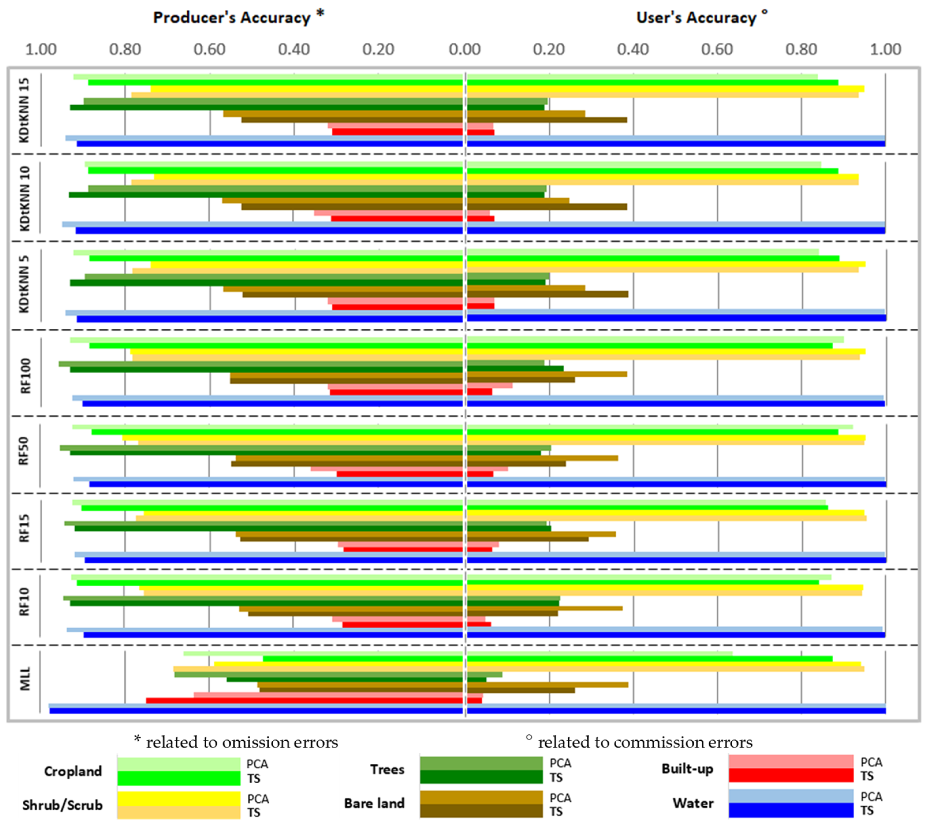
3.2. Assessment of Different Classification Methods and Input Parameters

As shown in Figure 6, the maps obtained with KDtKNN and RF with the different input parameters were quite similar, except for some differences in some classes, while the MLL classification showed many differences compared to KDtKNN and RF, and even showed an overestimation of the tree and building classes at the expense of the crop class. Indeed, the land use revealed discrepancies in the spatial distribution of some classes. However, the general aspect of the agricultural landscape was reproduced by most of the maps, except for the MLL maps, where cropland was highly underestimated. In addition to the speckled effect observed over the cropland and shrub/scrub classes, the MLL maps based on both feature inputs showed sparse trees and built-up areas, which were classified as cropland or shrub/scrub by the other RF and KDtKNN maps. For KDtKNN and RF, the PCA feature input gave almost similar results over all classes compared to the time-series (TS) feature input. This shows that MLL is very sensitive to the feature input, which has also been found by other studies. For example, Schulz et al. [31] showed that complex machine-learning classifiers such as SVM and RF were less sensitive to the choice of input features and performed better than MLL for mapping land use in a heterogeneous landscape in Niger, Sahel. As shown in Figure 6, RF produced the maps with the most accurate input parameters, namely by using 100 trees and 50 trees for PCA and TS feature inputs, respectively, while KDtKNN using 15 neighbors was the most accurate for both feature inputs.
Figure 7 shows the performance metrics of the different classifications and their processing times using a powerful machine. Of all the classifiers with different input parameters, RF using 50 trees slightly outperformed based on the overall accuracy (OA), kappa coefficient, and processing time (PT). It reached an OA of 84.28% (kappa = 0.73) using the S-1 time-series data as the input with 15.57 min in PT. Only MLL performed poorly for both the PCA and TS inputs, with a kappa of 0.43 and 0.42 and an OA not exceeding 0.63 and 0.62 using PCA and TS, respectively. The use of PCs achieved good results, as with those obtained using TS data with less processing time. This was especially true for the KDtKNN classifier, which took a lot of processing time by increasing the nearest neighbor parameter k. PCA gave better results than TS and resulted in a further decrease in the processing time from 130 min to 6 min (−95.3%) for KDtKNN using k = 5 (Figure 7), while this gain in processing time rose up to 57% for RF. Although KNN produced a good accuracy, the classifier remained slower and costlier in terms of time and memory. In fact, it required a high-performance machine with a large memory to store the training dataset [28]. In addition, the Euclidean distance used in the KNN algorithm was very sensitive to magnitudes, as features in the dataset that have high magnitudes will always have more weight than those with low magnitudes. This paper shows that the PCA of an S-1 time series can be used to address the limitation of KDtKNN not being suitable for high-dimensional datasets, leading to problems with machine time and performance.
Regarding the number of tree parameters of the RF, increasing it did not improve the performance much, but it caused an increase in the processing time as well as additional memory requirements. However, the number of 50 performed better than 100 with less processing time. These results corroborate those of Pham et al. [12], who found that using a tree number of 100, 200, 500, or 1000 gave the same performance with small differences depending on the land use classes. Moreover, Breiman [27] pointed out that using a large number of trees might be unnecessary because it does not improve performance, but it does not affect the accuracy of the classification. We noted that Thanh Noi and Kappas [32] combined S-1 radar and S-2 optical data and mapped almost the same classes as our research. However, in our case, a number of 50 trees was sufficient to give a satisfactory performance and fast computation time. Other authors such as Feng et al. [33] found that from 50 trees, RF could achieve stable and accurate results.
Concerning KDtKNN, as shown in Figure 7, increasing the value of the nearest neighbor parameter (k) did not improve the performance of the classification model, but it also consumed more processing time and more machine memory. KDtKNN with k = 5 was more efficient than k = 10 or 15. This finding corroborates several research studies [32,34], which proved that when k increases, the error of the KDtKNN classifier subsequently increases.
All of the classifications were assessed using the confusion matrix. A class-specific assessment was performed using user and producer accuracies (PA and UA), as reported in Figure 8. As noticed above on the produced maps, MLL showed a substantial underestimation of croplands and shrubs/scrubs, which was reflected in the low PA of these two classes compared to the RF and KDtKNN classifications. Low omission errors were reported for the built-up and water classes due to an overestimation of these classes using MLL. For all of the classifications, the user accuracies showed significant and steady commission errors on the built-up, bare land, and tree classes, which were emphasized more when using MLL. However, the cropland class, which is the class of interest for agricultural management applications, was well classified with few commission and omission errors using the different variants of KDtKNN and RF. The commission errors observed for the bare land, tree, and built-up classes were mainly related to the confusion between these classes by the classification models. To highlight this intra-class confusion, Table 2 presents the confusion matrix of the best classification model, namely RF using 50 trees.
In fact, there are two main confusions; the first is related to the commission errors of the bare land class, which was misclassified as shrub/scrub by all the classifications. In addition, some shrub/scrub areas were misclassified as bare land, trees, or a built-up area. This may be explained by the fact that shrub/scrub may show different states over time, namely double-bounce backscattering (which leads to confusion with trees or buildings) or low vegetation cover in dry periods, which leads to low backscattering and more surface scattering (and which causes confusion with bare land). The second is related to the confusion between the tree and built-up classes. The latter is mainly a reference to built-up areas classified as trees, which is not necessarily false since the built-up landscape in Senegal is mainly rural and buildings are sparse with lots of inclusion of trees within the built-up areas. The confusion of built-up areas with trees may be related to the double-bounce backscattering from trees and buildings.

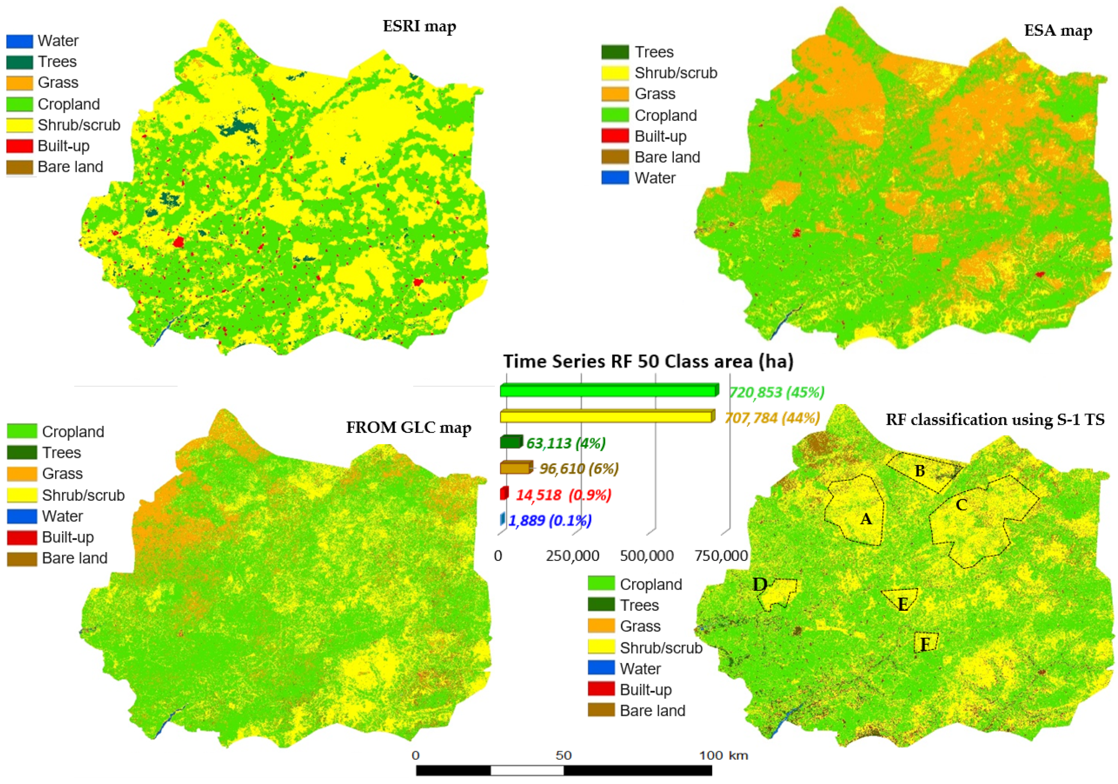
3.3. Land Cover Mapping

The results of the land cover mapping showed a good delineation of the crop area located mainly in the middle and the southwest of the Kaffrine region. Bare soil and shrubs (no agricultural area) were located mainly in the north. Figure 8 shows the best result obtained using RF50 compared with the existing maps from the ESA world cover, ESRI land cover, and FROM-GLC10 2017. As shown in Figure 9, the areas of the classes obtained by our RF50 classifier were 720,853 ha for the cropland class (45%), 707,784 ha for the shrub/scrub class (44%), 96,610 ha for the bare land class (6%), 63,113 ha for the tree class (4%), 14,518 ha for the built-up class (0.9%), and 1889 ha for the water class (0.1%). The obtained map explained the dominance of cropland, especially in the south and center of the Kaffrine region. These results show the importance of the Kaffrine region in agricultural production. In descending order of area and production, the crops in the Kaffrine region are mainly groundnuts, millet, sorghum, and corn. Each year, groundnuts represent almost half of the total cultivated area in the Kaffrine region. Indeed, the groundnut production area in the Kaffrine region is one of the leading agricultural regions in Senegal. Groundnut production was widely promulgated there by the government, and in 2019, this production represented up to 19% of the global groundnut production in Senegal. In the Kaffrine region, groundnuts are often rotated with millet, and the season is popularly considered to start in June and end in November.
The dominance of the shrub/scrub areas in the north of the region, as shown in the land cover map, is explained by the presence of three sylvo-pastoral reserves with low vegetation; the Mbégué Sylvo Pastoral Reserve in the northwestern region of Kaffrine, the Doli Sylvo Pastoral Reserve, and the Sine-Saloum Sylvo Pastoral Reserve in the northern region of Kaffrine. This may explain the dominance of this class in the obtained map. In addition, the LULC map shows the presence of many forests represented in the non-agricultural lands, such as Birkilane Forest in the center west; Sanian Forest, Delbi Forest, and Malem Hodar Forest in the center, the east, and the west of the region, respectively; and Maka Yop Forest, Birkilane Forest, Patte Forest, and Ndankou Forest located in the southwestern part of the region.
The built-up area class represents both the villages and the cities, as well as some bare soils. The regional pattern of built-up areas in Kaffrine is characterized by small scattered inland settlements, scattered trees within the settlements, and bare soils. As shown on the obtained map, these rural settlements are concentrated in the southern half of the Kaffrine region.
The water body class represents the Bao Bolon River, located in the southwestern region of Kaffrine, and the Saloum River in the western region of Kaffrine. In order to assess the suitability and reliability of our LULC map for agricultural management use, we compared it with recently available global land cover products. Figure 9 shows the comparison of the entire Kaffrine region, while Figure 10 shows a zoom-in over three zones with different landscapes.
The overall spatial distribution of the land use classes in the study area was derived from all maps except the FROM-GLC product. This product underestimated the area of the tree, shrub, and built-up classes that were misclassified as crops and/or grasses. Dong et al. [35] assessed the suitability of FROM-GLC10 data for understanding agricultural ecosystems in China, and found that FROM-GLC10 showed notable misclassifications between cropland, grassland, and forest. Hence, the suitability and reliability of FROM-GLC10 data for understanding agricultural ecosystems must be improved.
The ESRI product showed a clear delineation of the classes and did not show the speckle effect. This is not suitable for agricultural management purposes or local scale applications because the ESRI classification does not allow for intrinsic variability detection and does not account for spatial mixing (Figure 10). In general, the ESRI classification did not capture all of the agricultural land due to an overestimation of the shrub/scrub class (Figure 10—zones A, B, and C); this overestimation was mentioned in the work of Karra et al. [23]. In addition, an underestimation of the bare soil class was noticed on the ESRI product.
Concerning ESA, the first notable remark is that the grass class was greatly overestimated at the neglect of the shrub class; otherwise, the crop class was well and accurately mapped, as was the building class. The ESA product underestimated the tree class, which was often classified as scrubs as shown in Figure 10 (zones A and C). Of all three products, the ESA product appeared to be the most suitable and reliable to be used in the application of agricultural ecosystem management. This may be explained by the fact that ESA LC benefits from the synergy between SAR S-1 and optical S-2 satellite data.
At the crop-class level, our map achieved the same degree of accuracy and reliability as the ESA product using only the S-1 SAR data. A visual inspection of our map allowed us to see some improvements compared to the three products, notably the detection of trees, which were significantly underestimated by the three products. It also allowed us to detect the intrinsic variability between agricultural fields by avoiding the classification of small, scattered scrub areas as crops. However, some improvements should be expected to our classification in future work. These include the confusion between trees and buildings and a slight overestimation of the tree class at the cost of the scrub class. The pattern of built-up areas corresponds to scattered small inland villages, where very few temporal changes (in terms of SAR backscattering) can be perceived by the VH backscatters of the S-1 satellite. This makes it difficult to separate the classes that form the Senegalese rural landscape, which is characterized by a scattered and very sparse settlements with the inclusion of trees and shrubs between the houses. Hence, the discrimination of the built-up area, at a regional scale, depends highly on the contrast between the settlements themselves and their environment.
LULC mapping is one of the tools used for natural resource management and for developing solutions to increase agricultural production sustainably and significantly. Land use maps are important for a variety of applications, such as digital soil mapping, agricultural monitoring, and informed policy, development, planning, and resource management decisions. However, creating consistent and relevant agricultural land use maps using optical remote-sensing imagery remains challenging due to the diversity and complexity of the landscape and the near impossibility of a continuous and free satellite image acquisition in some cloudy countries. Several studies have used S-1 data for land cover mapping, demonstrating a lower potential of S-1 for LULC classification and finding that the S-1 approach alone performed poorly compared to the S-1 and optical S-2 data combined or an S-2 optical approach. In this study, the proposed approach using only radar data, namely the S-1 time-series data, gave a good performance with an overall accuracy of 0.84. Several authors have achieved a similar or higher accuracy up to 92%, as mentioned in the introduction, but this was by integrating the S-2 optical data. An improvement in the overall accuracy using only the S-1 data could be achieved by increasing the S-1 input data, i.e., derived data such as polarimetric parameters, or polarizations other than VH. Another way of improvement consists of using a deep-learning classification in the case of the availability of a large database of ground truth samples for the training of the classification model.
This research proposed a cost-effective method using machine-learning for improving agricultural land use/cover classification by using only SAR satellite imagery. Indeed, we successfully mapped the land use and land cover in agricultural areas in the Kaffrine region of Senegal using a set of SAR C-band VH S-1 time-series data. The RF gave the best mapping results. However, we demonstrated the usefulness of combining PCA as a feature input into the KDtKNN classifier, which resulted in almost the same performance as RF in terms of minimizing the processing time and computing resources. This allowed our approach to be implemented for regional- or national-scale mapping using large Sentinel-1 radar data without compromising computer resources. Our approach is also simple, fast, and uses a single source of data, which favors its use on cloud-computing servers such as Google Earth Engine.
The results show that the ML classification of the S-1 SAR data alone performed well in a very large area and may be used for other sub-Saharan and Sahel countries, as well as other similar regions. However, it could also be tested for other countries that experience frequent clouds. In future work, the suggested approach can be tested and validated over multiple landscapes to assess its generalizability. Besides, the approach should be used for LULC, for change detection, and for assessing the other S-1 polarization, especially for the LULC applications related to the study of the vegetation state and structure.

4. Conclusions

In this paper, we suggested a satisfactory method using only SAR S-1 data for LULC mapping, especially in agricultural areas. We used a set of SAR C-band S-1 time-series data over our area of interest, located in the Kaffrine region of Senegal. We assessed the performance and the processing time of three machine-learning classifiers applied on two inputs. In fact, we applied the RF, KDtKNN, and MLL classifiers using two separate inputs, namely a set of monthly S-1 time-series data acquired during 2020 and the principal components (PCs) of the time-series dataset. In addition, the RF and KDtKNN classifiers were processed using different tree numbers for RF (10, 15, 50, and 100) and different neighbor numbers for KDtKNN (5, 10, and 15).
As a result, the RF classification using S-1 time-series data gave the best performance in terms of accuracy (overall accuracy = 0.84, kappa = 0.73) with 50 trees in 15.5 min of processing time. However, the processing time was very slow compared to KDtKNN, which also gave a good accuracy (overall accuracy = 0.82, kappa = 0.68) in 6.3 min of processing time using PCA input. Increasing the tree number for the RF classification slightly enhanced the classification accuracy and significantly slowed the processing time, while increasing the neighbor number in the KDtreeKNN classifier notably increased the processing time and slightly decreased the accuracy. Furthermore, our results were compared with the FROM-GLC, ESRI, and ESA world cover maps and showed significant improvements for some land use and land cover classes.
This paper showed the performance of machine-learning classifiers for improving land use/cover classification using SAR satellite imagery as a single data source. This can be used for large-area land cover mapping in sub-Saharan agricultural areas that experience frequent clouds. Besides that, this research provides insights into the selection of classifiers and the feature input of the classifiers for using a large S-1 dataset for LULC mapping without the integration of optical satellite data. The results showed the suitability and reliability of our land cover map based on only VH S-1 GRD data for assisting with agricultural management in sub-Saharan regions.

Author Contributions

Conceptualization, S.D., M.R., M.H. and R.L.; data curation, S.D.; formal analysis, S.D.; investigation, S.D.; methodology, S.D., M.R., M.H. and R.L.; project administration, M.R. and M.H.; resources, S.D. and R.L.; software, S.D. and R.L.; supervision, M.R. and M.H.; validation, S.D., M.R., M.H. and R.L.; visualization, S.D.; writing—original draft, S.D.; writing—review and editing, S.D., M.R., M.H. and R.L. All authors have read and agreed to the published version of the manuscript.

Funding

This research received no external funding.

Data Availability Statement

Not applicable.

Acknowledgments

The authors thank the Faculty of Sciences at Ben M’sik, Hassan II University of Casablanca for its logistical support. In addition, the authors extend many thanks to ESA for providing the S-1 data free of charge.

Conflicts of Interest

The authors declare no conflict of interest.

References

  1. FAO. The Future of Food and Agriculture: Trends and Challenges; Food and Agriculture Organization of the United Nations: Rome, Italy, 2017; p. 163. [Google Scholar]
  2. Thenkabail, P.S. Global Croplands and their Importance for Water and Food Security in the Twenty-first Century: Towards an Ever Green Revolution That Combines a Second Green Revolution with a Blue Revolution. Remote Sens. 2010, 2, 2305–2312. [Google Scholar] [CrossRef] [Green Version]
  3. Fritz, S.; See, L.; Bayas, J.C.L.; Waldner, F.; Jacques, D.; Becker-Reshef, I.; Whitcraft, A.; Baruth, B.; Bonifacio, R.; Crutchfield, J.; et al. A comparison of global agricultural monitoring systems and current gaps. Agric. Syst. 2019, 168, 258–272. [Google Scholar] [CrossRef]
  4. Saah, D.; Tenneson, K.; Poortinga, A.; Nguyen, Q.; Chishtie, F.; Aung, K.S.; Markert, K.N.; Clinton, N.; Anderson, E.R.; Cutter, P.; et al. Primitives as building blocks for constructing land cover maps. Int. J. Appl. Earth Obs. Geoinf. 2020, 85, 101979. [Google Scholar] [CrossRef]
  5. Ngo, K.D.; Lechner, A.M.; Vu, T.T. Land cover mapping of the Mekong Delta to support natural resource management with multi-temporal Sentinel-1A synthetic aperture radar imagery. Remote Sens. Appl. Soc. Environ. 2020, 17, 100272. [Google Scholar] [CrossRef]
  6. Nijhawan, R.; Joshi, D.; Narang, N.; Mittal, A.; Mittal, A. A Futuristic Deep Learning Framework Approach for Land Use-Land Cover Classification Using Remote Sensing Imagery. In Advanced Computing and Communication Technologies; Springer: Singapore, 2019; pp. 87–96. [Google Scholar]
  7. Zhang, C.; Li, X. Land Use and Land cover Mapping in the Era of Big Data. Land 2022, 11, 1692. [Google Scholar] [CrossRef]
  8. Ohki, M.; Shimada, M. Large-Area Land Use and Land Cover Classification with Quad, Compact, and Dual Polarization SAR Data by PALSAR-2. IEEE Trans. Geosci. Remote Sens. 2018, 56, 5550–5557. [Google Scholar] [CrossRef]
  9. Dingle Robertson, L.; Davidson, A.M.; McNairn, H.; Hosseini, M.; Mitchell, S.; de Abelleyra, D.; Verón, S.; le Maire, G.; Plannells, M.; Valero, S.; et al. C-band synthetic aperture radar (SAR) imagery for the classification of diverse cropping systems. Int. J. Remote Sens. 2020, 41, 9628–9649. [Google Scholar] [CrossRef]
  10. Prudente, V.H.R.; Sanches, I.D.; Adami, M.; Skakun, S.; Oldoni, L.V.; Xaud, H.A.M.; Xaud, M.R.; Zhang, Y. SAR Data for Land Use Land Cover Classification in a Tropical Region with Frequent Cloud Cover. In Proceedings of the IGARSS 2020—2020 IEEE International Geoscience and Remote Sensing Symposium, Waikoloa, HI, USA, 26 September–2 October 2020; pp. 4100–4103. [Google Scholar]
  11. Denize, J.; Hubert-Moy, L.; Betbeder, J.; Corgne, S.; Baudry, J.; Pottier, E. Evaluation of Using Sentinel-1 and -2 Time-Series to Identify Winter Land Use in Agricultural Landscapes. Remote Sens. 2019, 11, 37. [Google Scholar] [CrossRef] [Green Version]
  12. Pham, L.H.; Pham, L.T.H.; Dang, T.D.; Tran, D.D.; Dinh, T.Q. Application of Sentinel-1 data in mapping land-use and land cover in a complex seasonal landscape: A case study in coastal area of Vietnamese Mekong Delta. Geocarto Int. 2021, 37, 3743–3760. [Google Scholar] [CrossRef]
  13. Fonteh, M.L.; Theophile, F.; Cornelius, M.L.; Main, R.; Ramoelo, A.; Cho, M.A. Assessing the Utility of Sentinel-1 C Band Synthetic Aperture Radar Imagery for Land Use Land Cover Classification in a Tropical Coastal Systems When Compared with Landsat 8. J. Geogr. Inf. Syst. 2016, 8, 495–505. [Google Scholar] [CrossRef]
  14. Kpienbaareh, D.; Sun, X.; Wang, J.; Luginaah, I.; Bezner Kerr, R.; Lupafya, E.; Dakishoni, L. Crop Type and Land Cover Mapping in Northern Malawi Using the Integration of Sentinel-1, Sentinel-2, and PlanetScope Satellite Data. Remote Sens. 2021, 13, 700. [Google Scholar] [CrossRef]
  15. Carrasco, L.; O’Neil, A.W.; Morton, R.D.; Rowland, C.S. Evaluating Combinations of Temporally Aggregated Sentinel-1, Sentinel-2 and Landsat 8 for Land Cover Mapping with Google Earth Engine. Remote Sens. 2019, 11, 288. [Google Scholar] [CrossRef] [Green Version]
  16. Hu, B.; Xu, Y.; Huang, X.; Cheng, Q.; Ding, Q.; Bai, L.; Li, Y. Improving Urban Land Cover Classification with Combined Use of Sentinel-2 and Sentinel-1 Imagery. ISPRS Int. J. Geo-Inf. 2021, 10, 533. [Google Scholar] [CrossRef]
  17. Steinhausen, M.J.; Wagner, P.D.; Narasimhan, B.; Waske, B. Combining Sentinel-1 and Sentinel-2 data for improved land use and land cover mapping of monsoon regions. Int. J. Appl. Earth Obs. Geoinf. 2018, 73, 595–604. [Google Scholar] [CrossRef]
  18. Lopes, M.; Frison, P.-L.; Crowson, M.; Warren-Thomas, E.; Hariyadi, B.; Kartika, W.D.; Agus, F.; Hamer, K.C.; Stringer, L.; Hill, J.K.; et al. Improving the accuracy of land cover classification in cloud persistent areas using optical and radar satellite image time series. Methods Ecol. Evol. 2020, 11, 532–541. [Google Scholar] [CrossRef]
  19. Li, Q.; Qiu, C.; Ma, L.; Schmitt, M.; Zhu, X.X. Mapping the Land Cover of Africa at 10 m Resolution from Multi-Source Remote Sensing Data with Google Earth Engine. Remote Sens. 2020, 12, 602. [Google Scholar] [CrossRef] [Green Version]
  20. USAID. Climate Change Adaptation in Senegal; InTech: Singapore, 2012; ISBN 978-953-51-0747-7. [Google Scholar]
  21. ANSD. Agence Nationale de la Statistique et de la Démographie; ANSD: Singapore, 2016. [Google Scholar]
  22. Dobrinić, D.; Gašparović, M.; Medak, D. Sentinel-1 and 2 Time-Series for Vegetation Mapping Using Random Forest Classification: A Case Study of Northern Croatia. Remote Sens. 2021, 13, 2321. [Google Scholar] [CrossRef]
  23. Karra, K.; Kontgis, C.; Statman-Weil, Z.; Mazzariello, J.C.; Mathis, M.; Brumby, S.P. Global land use/land cover with Sentinel 2 and deep learning. In Proceedings of the 2021 IEEE International Geoscience and Remote Sensing Symposium IGARSS, Brussels, Belgium, 11–16 July 2021; pp. 4704–4707. [Google Scholar]
  24. Gong, P.; Liu, H.; Zhang, M.; Li, C.; Wang, J.; Huang, H.; Clinton, N.; Ji, L.; Li, W.; Bai, Y.; et al. Stable classification with limited sample: Transferring a 30-m resolution sample set collected in 2015 to mapping 10-m resolution global land cover in 2017. Sci. Bull. 2019, 64, 370–373. [Google Scholar] [CrossRef] [Green Version]
  25. Zanaga, D.; Van De Kerchove, R.; De Keersmaecker, W.; Souverijns, N.; Brockmann, C.; Quast, R.; Wevers, J.; Grosu, A.; Paccini, A.; Vergnaud, S.; et al. ESA WorldCover 10 m 2020 v100. 2021. Available online: https://doi.org/10.5281/zenodo.5571936 (accessed on 28 July 2022).
  26. Pereira, L.O.; Freitas, C.C.; Sant´Anna, S.J.S.; Reis, M.S. Evaluation of Optical and Radar Images Integration Methods for LULC Classification in Amazon Region. IEEE J. Sel. Top. Appl. Earth Obs. Remote Sens. 2018, 11, 3062–3074. [Google Scholar] [CrossRef]
  27. Breiman, L. Random forests. Mach. Learn. 2001, 45, 5–32. [Google Scholar] [CrossRef]
  28. Meng, Q.; Cieszewski, C.J.; Madden, M.; Borders, B.E. K Nearest Neighbor Method for Forest Inventory Using Remote Sensing Data. GIScience Remote Sens. 2007, 44, 149–165. [Google Scholar] [CrossRef]
  29. Cao, X.; Wei, C.; Han, J.; Jiao, L. Hyperspectral Band Selection Using Improved Classification Map. IEEE Geosci. Remote Sens. Lett. 2017, 14, 2147–2151. [Google Scholar] [CrossRef] [Green Version]
  30. Paul, S.; Kumar, D.N. Evaluation of Feature Selection and Feature Extraction Techniques on Multi-Temporal Landsat-8 Images for Crop Classification. Remote Sens. Earth Syst. Sci. 2019, 2, 197–207. [Google Scholar] [CrossRef]
  31. Schulz, D.; Yin, H.; Tischbein, B.; Verleysdonk, S.; Adamou, R.; Kumar, N. Land use mapping using Sentinel-1 and Sentinel-2 time series in a heterogeneous landscape in Niger, Sahel. ISPRS J. Photogramm. Remote Sens. 2021, 178, 97–111. [Google Scholar] [CrossRef]
  32. Thanh Noi, P.; Kappas, M. Comparison of Random Forest, k-Nearest Neighbor, and Support Vector Machine Classifiers for Land Cover Classification Using Sentinel-2 Imagery. Sensors 2018, 18, 18. [Google Scholar] [CrossRef] [Green Version]
  33. Feng, Q.; Liu, J.; Gong, J. UAV Remote Sensing for Urban Vegetation Mapping Using Random Forest and Texture Analysis. Remote Sens. 2015, 7, 1074. [Google Scholar] [CrossRef] [Green Version]
  34. Qian, Y.; Zhou, W.; Yan, J.; Li, W.; Han, L. Comparing Machine Learning Classifiers for Object-Based Land Cover Classification Using Very High Resolution Imagery. Remote Sens. 2015, 7, 153. [Google Scholar] [CrossRef]
  35. Dong, S.; Gao, B.; Pan, Y.; Li, R.; Chen, Z. Assessing the suitability of FROM-GLC10 data for understanding agricultural ecosystems in China: Beijing as a case study. Remote Sens. Lett. 2020, 11, 11–18. [Google Scholar] [CrossRef]
Figure 1. Map of the study area in the Kaffrine region with its four departments.
Remotesensing 15 00065 g001
Figure 2. Flowchart showing the technical approach used to evaluate agricultural LULC mapping using S-1 data.
Remotesensing 15 00065 g002
Figure 3. The ground truth data collected. The samples were not balanced, with 123,850 pixels (1238.5 ha) of crops, 273,600 pixels (27,360 ha) of shrubs/scrubs, 8540 pixels (85.4 ha) of trees, 11,840 pixels (118.4 ha) of bare soil, 2610 pixels (26.1 ha) of built-up area, and 10,840 pixels (108.4 ha) of water. From each class, we used 40% of the pixels for training the classifiers, and the remaining 60% were used for validation.
Remotesensing 15 00065 g003
Figure 4. The PCA eigenvalue plot obtained.
Remotesensing 15 00065 g004
Figure 5. Multitemporal composite of S-1 data (RGB:June/October/January) and color composite of PCA (RGB:PC1/PC2/PC3) over the Kaffrine region.
Remotesensing 15 00065 g005
Figure 6. The best results for land cover maps of Kaffrine obtained from RF, KDtKNN, and MLL applied to the S-1 time-series (TS) data (left) and PCs (right). RF using 100 trees and 50 trees was the most accurate for PCs and time series, respectively, while KDtKNN using 15 neighbors was the most accurate for both feature inputs.
Remotesensing 15 00065 g006
Figure 7. Comparison of different classifiers using overall accuracy (OA), kappa coefficient, and processing time. Note that the specifications of the computer used were quite high, namely Intel Core i7 10th generation 10,700 K, CPU 3.80 GHz, and 64 Go RAM.
Remotesensing 15 00065 g007
Figure 8. Class-specific assessment showing the user and producer accuracies of all classifications using TS and PCA input features. RF: random forest using different numbers of trees—10, 15, 50, or 100; KDtKNN: K-D tree KNN using different numbers of nearest neighbors—5, 10, or 15; and MLL: maximum likelihood. Each class shows two input datasets using two tones: bright (upper) and dark (lower) for PCA and time-series (TS) inputs, respectively.
Remotesensing 15 00065 g008
Figure 9. Comparison between our land cover map of Kaffrine obtained from RF50 and other available land-use products; ESRI, ESA, and FROM-GLC land cover maps. A: Mbégué Sylvo Pastoral Reserve, B: Doli Sylvo Pastoral Reserve, C: Sine-Saloum Sylvo Pastoral Reserve, D: Birkilane Forest, E: Delbi Forest, and F: Malem Hodar Forest.
Remotesensing 15 00065 g009
Figure 10. Detailed comparison between our RF50 land cover map with the ESRI, ESA, and FROM-GLC land cover maps over three local zones representing different agricultural landscapes within the Kaffrine region.
Remotesensing 15 00065 g010
Table 1. The dates for radar image acquisitions.
MonthDay (Scene 1,4/Scene 2,3)PolarizationOrbitMean Incidence Angle
January04-01-2020/11-01-2020VHAscending38.415
February04-02-2020/09-02-2020VHAscending38.415
March11-03-2020/16-03-2020VHAscending38.430
April04-04-2020/09-04-2020VHAscending38.420
May03-05-2020/10-05-2020VHAscending38.435
June15-06-2020/20-06-2020VHAscending38.434
July21-07-2020/26-07-2020VHAscending38.421
August14-08-2020/19-08-2020VHAscending38.418
September19-09-2020/24-09-2020VHAscending38.434
October13-10-2020/18-10-2020VHAscending38.434
November23-11-2020/28-11-2020VHAscending38.416
December24-12-2020/29-12-2020VHAscending38.417
Table 2. Confusion matrix of the RF50 classifier.
Reference Data
ClassesCroplandShrub/
Scrub
TreesBare LandBuilt-upWaterRow TotalU AccuracyErrors of Commission
Cropland96,2997731551220104,5490.927.89
Shrub/Scrub6891166,5316217572080175,4490.955.08
Trees58822,0726120191148029,9470.2079.56
Bare land383363402713071574450.3663.56
Built-up6639022720764074070.1089.69
Water0190180858386201.000.43
Column Total104,167206,3776414503921229298333,417
P Accuracy0.920.810.950.540.360.92Overall Accuracy0.84
Errors of Omission7.5519.314.5846.1664.007.69Kappa Coefficient0.73
Disclaimer/Publisher’s Note: The statements, opinions and data contained in all publications are solely those of the individual author(s) and contributor(s) and not of MDPI and/or the editor(s). MDPI and/or the editor(s) disclaim responsibility for any injury to people or property resulting from any ideas, methods, instructions or products referred to in the content.

