Article

LSTM-VAE for Temporal Anomaly Detection in Drone Trajectory Analysis: A Comparative Study for Critical Infrastructure Protection

by
Hari Hara Babu Saripalli
1,*,
Jyothsna Laxmi Saripalli
1,
Leonel Lagos
1,2,* and
Himanshu Upadhyay
1,3
1
Applied Research Center, Florida International University, Miami, FL 33174, USA
2
Moss School of Construction, Florida International University, Miami, FL 33174, USA
3
Department of Electrical & Computer Engineering, Florida International University, Miami, FL 33174, USA
*
Authors to whom correspondence should be addressed.
Future Internet 2026, 18(6), 301; https://doi.org/10.3390/fi18060301
Submission received: 13 April 2026 / Revised: 25 May 2026 / Accepted: 29 May 2026 / Published: 3 June 2026
(This article belongs to the Special Issue Wireless Sensor Networks and Internet of Things—2nd Edition)

Abstract

Unauthorized commercial drone activity around critical infrastructure motivates the development of trajectory-level anomaly detection. We present a rigorous benchmarking study of variational autoencoder methods for drone trajectory anomaly detection in a simulated nuclear facility protection scenario, evaluating six methods (bidirectional LSTM-VAE, unidirectional LSTM-VAE, fully connected VAE, standard autoencoder, One-Class SVM, Isolation Forest) on 2500 trajectories using identical raw features and training pipelines. Across five random seeds, all VAE variants achieve AUC-ROC of approximately 0.92 versus 0.73 to 0.80 for the non-VAE baselines, isolating variational regularization rather than bidirectionality or temporal encoding alone as the dominant performance driver in this domain. Building on this benchmark, we propose a domain-aware LSTM-VAE incorporating two facility-specific architectural elements: a polar coordinate input representation expressing trajectories relative to the protected facility and a distance-weighted reconstruction loss that allocates model capacity toward near-facility timesteps. The domain-aware variant achieves AUC-ROC of 0.962 ± 0.007 on the original test set and 0.973 ± 0.005 on an augmented hard anomalies test set, a 3 to 4 percentage-point improvement over generic VAE methods at no additional parameter cost. A bootstrap evaluation under 99:1 class imbalance confirms that the domain-aware variant maintains its precision advantage at low false positive rate operating points.

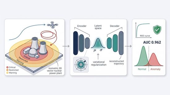
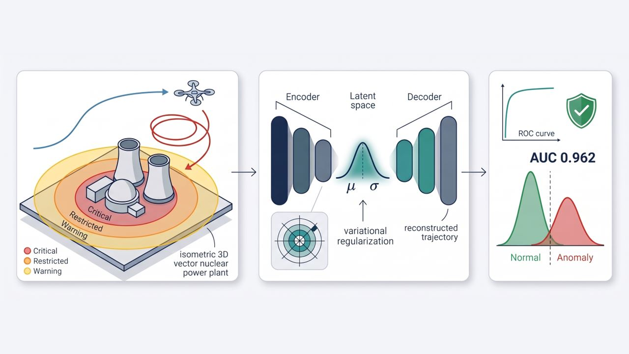
Graphical Abstract

1. Introduction

The rapid development of commercial unmanned vehicles, also referred to as drones, has impacted various industries such as logistics, agriculture, film, and inspection. However, this proliferation has also introduced security risks for critical infrastructure. In U.S. policy, critical infrastructure is formally defined under the 2024 National Security Memorandum on Critical Infrastructure Security and Resilience (NSM-22), which reaffirms the sixteen sectors originally identified by Presidential Policy Directive 21, including chemical facilities, commercial facilities, communications, critical manufacturing, dams, defense industrial base, emergency services, energy, financial services, food and agriculture, government facilities, healthcare and public health, information technology, nuclear reactors and materials, transportation systems, and water and wastewater systems, as assets, systems, and networks whose incapacitation or destruction would have a debilitating effect on national security, economic security, public health, or safety [1]. Residential buildings, however densely populated, fall outside this designated set; this study targets the nuclear reactors and materials sector specifically, where unauthorized drone access carries operational and physical consequences distinct from civilian density risk. The unauthorized use of drones over such facilities, for surveillance, transport of harmful payloads, or disruption of operations, has become a documented operational concern. The unauthorized use of drones includes surveillance, transportation of harmful substances, or disruption of operations. The affordability and accessibility of commercial drones have enabled malicious actors to exploit them for unauthorized purposes, presenting a significant challenge for security professionals worldwide [2]. In 2024, the U.S. Nuclear Regulatory Commission updated its regulations to mandate that nuclear power plant licensees report drone sightings over their facilities [3], and over 350 unauthorized drone incursions were documented across more than 100 U.S. military installations within a single year [4].
In the past, drones were located through the use of radar detection, analysis of radio signals, acoustic signatures, and computer vision. While these approaches have had varying degrees of success, each of these approaches has a major limitation. Radar detection is difficult for drones flying low, especially if they are small. The drone also needs to be transmitting signals for the radio signal detection to work. It does not work for drones that are already set to fly autonomously. Acoustic detection is difficult because of the noise from the outside world. It does not work very well at a distance. Weather and camera coverage are big factors in how well you can see things. Recent comprehensive surveys have cataloged the strengths and limitations of each modality in detail [5,6]. Therefore, a new means of detection is being developed, focusing on how drones behave. More broadly, machine learning and artificial intelligence techniques have demonstrated significant potential across intelligent transportation and infrastructure protection systems [7], motivating their application to drone trajectory analysis.
A complementary approach is to analyze changes in a drone’s flight pattern over time. The underlying idea is that anomalous drone flights differ from nominal ones. For a delivery drone, nominal flights are efficient point-to-point routes; for a survey drone, nominal flights are regular grid patterns; for a recreational drone, nominal flights are loosely structured but stay clear of restricted airspace. Anomalous patterns, in contrast, include sustained loitering near protected zones, straight-line approaches toward a restricted area, and evasive zigzag patterns intended to avoid detection. Anomaly detection learns the statistical envelope of nominal flights and uses it to identify departures from that envelope, which may indicate a threat.
Anomaly detection using variational autoencoders (VAEs) [8,9] provides an unsupervised alternative for learning to detect anomalies from non-anomalies. Unlike supervised autoencoders that are trained from examples of anomalous inputs, standard VAEs do not necessarily have to train on anomalous samples. However, typically, fully connected architectures are used, which treat trajectories as feature vectors (i.e., losing the temporal nature of flight paths). Anomalous behaviors (e.g., sudden changes in speed, reversing heading, approaching then retreating, vertiginous movements to which the drone has no business losing itself, etc.) evolve as temporal patterns, and are hence beyond what static feature representations might capture. LSTMs [10] leverage a simple gating mechanism to encode memory of long-range temporal dependencies. Their architecture, applied to the encoder in the VAE paradigm, provides a principled way of enriching latent representation learning with temporal knowledge.
This paper takes a benchmarking-first approach to drone trajectory anomaly detection. Rather than asserting the superiority of any single architecture, we systematically compare three VAE variants and three non-VAE baselines under identical conditions to identify which architectural property, variational regularization, temporal encoding, or bidirectionality, drives detection performance. Building on the empirical findings of this benchmark, we then introduce a domain-aware LSTM-VAE that incorporates facility-specific architectural elements designed to address the geometric, kinematic, and regulatory characteristics of trajectory data near a protected site, responding to the observation that generic VAE-LSTM architectures lack mechanisms tailored to airspace protection contexts.
Our contributions are as follows: (i) a rigorous multi-seed benchmark of six anomaly detection methods (bidirectional LSTM-VAE, unidirectional LSTM-VAE, fully connected VAE, standard autoencoder, One-Class SVM, and Isolation Forest), evaluated on identical raw trajectory features with consistent training pipelines and explicit GPU-RNG seeding for reproducibility; (ii) an empirical attribution of the performance gap to variational regularization rather than bidirectionality or LSTM-specific temporal encoding, demonstrated by the near-equivalent AUC of all three VAE variants and the consistent gap to non-VAE baselines; (iii) a domain-aware LSTM-VAE that incorporates a polar coordinate input representation and a distance-weighted reconstruction loss tailored to the geometric and operational characteristics of facility protection scenarios, providing a measurable improvement over generic VAE methods at no additional parameter cost; (iv) a deployment-realistic evaluation under 99:1 class imbalance via a 1000-iteration bootstrap, characterizing precision at low FPR operating points relevant to security operations; (v) an augmented hard anomaly test set with four additional threat classes (subtle far-loitering, delayed approach, path mimicking, and multi-segment coordinated approaches) to probe robustness beyond the original taxonomy.
The remainder of this paper is organized as follows: Section 2 reviews related work, Section 3 describes our methodology, Section 4 details the experimental setup, Section 5 presents results, Section 6 provides discussion, and Section 7 concludes with future directions.

2. Related Work

2.1. Drone Detection and Classification

To counter the ever-growing threat of drones, substantial research has been conducted on detection and classification using physical modality signals, radar returns, RF emissions, acoustic signatures, and visual imagery. The trajectory signals on which this paper focuses (positions, velocities, kinematic derivatives, and facility-relative quantities) are defined formally in Section 3.1 and Table 1; the present section restricts itself to the physical modality literature, which provides the operational context against which trajectory-based behavioral detection is positioned as a complementary modality. Machine learning and AI methods have been widely reviewed for intelligent transportation and infrastructure applications [7], with drone detection emerging as a critical sub-domain. The most effective method to identify drones and differentiate them from birds and other flying objects is by the use of radar technology. This is achieved through micro-Doppler signatures generated by the rotation of the propellers, with comprehensive frequency-domain and statistical signal-processing approaches surveyed in [11]. Detection remains challenging for consumer-grade UAVs because of their low radar cross-section, typically 0.01 to 0.1 m2 for mini and micro-UAV classes [5,6]. Ground clutter and the operational tendency of small UAVs to fly at low altitudes further complicate radar discrimination, especially in cluttered urban or industrial environments. A recent review of cybersecurity and AI challenges in UAV systems highlights that AI-driven anomaly detection represents a key emerging countermeasure for securing UAV operations around critical infrastructure [12].
Acoustic detection systems involve the use of different sounds made by the motors and the propellers of drones. In a controlled environment, machine learning classifiers can achieve high accuracy in the classification and detection of drones. On the other hand, the use of acoustic detection is normally limited to a certain distance, which is normally less than 500 m, and the use of acoustic detection in a city environment is not effective due to the high number of sound sources. Additionally, the accuracy of the detection can vary significantly depending on the prevailing wind.
To detect drones, computer vision is also used, and the most effective method is the use of deep learning algorithms for object detection. The use of convolutional neural networks is effective in a controlled environment, but in real-world scenarios, the use of computer vision is normally affected by a number of factors, including changes in lighting, weather, low resolution of the camera, and difficulties in seeing the drones due to their size and the distance from the drone. Pan–tilt–zoom cameras can also increase the detection range, but they can also make the detection more complicated.
RF detection looks at the control signals and telemetry transmissions that drones send and receive from their operators. This method can help you figure out exactly what kind of drone it is and, in some cases, where the operator is. But RF detection does not work on autonomous drones that fly to pre-programmed waypoints without communicating with other devices, and smart enemies might use frequency hopping or encrypted transmissions. A comprehensive survey on the RF-based detection, classification, and tracking of UAVs using radars and communication systems has elaborated on the above-mentioned limitations [11]. The multi-sensor fusion techniques involving the use of RF signals, acoustic signals, and deep neural networks have also been found to provide promising results to overcome the limitations of the individual sensor techniques [13].
The use of behavioral analysis techniques involving the examination of the trajectory of the object has received relatively less attention; however, recent studies have highlighted the potential of the technique as an additional means of object detection. We refer to operationally compliant trajectories, those obeying the relevant airspace regulations and the kinematic constraints of small unmanned aircraft systems, as nominal flights. In the U.S. civilian context this is operationally defined by 14 CFR Part 107 [14], which establishes maximum altitude (400 ft AGL), maximum groundspeed (87 knots/100 mph), restricted airspace prohibitions, and visual-line-of-sight requirements; international authorities (ICAO, EASA) provide analogous frameworks. A nominal flight in our facility protection context is one that respects both these regulatory constraints and the airspace boundaries imposed by the protected site. The behavioral analysis paradigm aims to recognize departures from this nominal envelope without enumerating every possible departure, which is the role that one-class learning plays. The basic idea is to use the fact that the behavioral pattern may reveal malicious intent even if physical means of object detection are employed to detect the object. To differentiate between a delivery drone and a malicious object, it is important to understand the context of the flight pattern. Recent studies on the use of AI to improve intrusion detection techniques for the overall UAV system have highlighted the fact that the use of behavioral techniques involving trajectory is still an underexplored area compared to physical object detection techniques [15].

2.2. Variational Autoencoders for Anomaly Detection

Kingma and Welling [9] introduced the variational autoencoder (VAE) as a probabilistic generative model that learns a structured latent representation of high-dimensional data. Where a standard autoencoder maps each input deterministically to a single latent code, a VAE maps each input to a probability distribution, typically a multivariate Gaussian parameterized by an encoder neural network, and trains a decoder to reconstruct the input from samples drawn from this distribution. Backpropagation through the sampling step is enabled by the reparameterization trick, which expresses the random sample as a deterministic function of the distribution parameters and an auxiliary noise variable. Training optimizes a combined objective: a reconstruction term that rewards faithful decoding and a Kullback–Leibler divergence term that constrains the encoder distribution to remain close to a standard normal prior. The latter term acts as a regularizer that organizes the latent space into a smooth, contiguous geometry rather than a disconnected set of point codes; in anomaly detection, this regularization is what enables out-of-distribution inputs to produce systematically larger reconstruction errors than in-distribution ones.
An and Cho [8] proposed the formalization of the variational autoencoders for anomaly detection by proposing the use of the probability of reconstruction as a measure of anomaly detection. This is based on the fact that the normal data, assumed to follow a normal distribution, can be reconstructed with high probability, while anomalies, being outside the distribution, will have low probability of reconstruction, leading to poor reconstruction. This unsupervised method is useful when there are no examples of anomalies, such as threats, which are unusual or do not represent future threats.
VAE-based anomaly detection has been successfully used in many fields. In the manufacturing sector, the VAE detects anomalies in the products by learning the expected look of the manufactured items [16]. In the cyber world, the VAE detects intrusions by analyzing the normal flow of the network. The VAE used in the video surveillance sector detects anomalies by analyzing the way the scenes change over time. The VAE detects anomalies by finding unusual activities in the scenes [17]. In the medical sector, the VAE detects anomalies by finding unusual patterns in the images or physiological signals. VAE is preferred in the detection of anomalies where it is difficult to enumerate the anomalies, as it can create new anomalies.
A recent evaluation of reconstruction-based deep learning methods for multivariate time series anomaly detection confirmed that VAE-based approaches consistently outperform standard autoencoders in generalization to unseen anomaly types [18]. Furthermore, VAE and LSTM-based architectures have been applied to ADS-B flight trajectory anomaly detection, though recent work has also revealed their vulnerability to adversarial attacks in air traffic management contexts [19].
The β-VAE variant added a way to change the weight on the KL divergence term, which made it possible to control the balance between reconstruction quality and latent space regularization [20]. Higher β values make it easier to create representations that are not tangled up, but they may lose accuracy in reconstruction.
In most cases, moderate β value usage is most effective in detecting anomalies since they offer a balance between the importance of reconstruction and a properly regularized latent space that is compatible with more than just the training data. A recent comprehensive survey on “Deep Learning for Time Series Anomaly Detection” classifies VAE-based methods as one of the most important reconstruction-based methods in time series anomaly detection, particularly for unsupervised methods [21]. However, there are some limitations in using conventional VAE methods in capturing long-periodic heterogeneous data and detailed short-periodic trends simultaneously [22]. A comprehensive taxonomy for “Deep Anomaly Detection for Multivariate Time Series” classifies various methods, including VAE-based, GAN-based, Transformer-based, and diffusion-based reconstruction methods, in which our proposed method is included [23].

2.3. Temporal Models for Sequential Anomaly Detection

Hochreiter and Schmidhuber [10] came up with Long Short-Term Memory (LSTM) networks, which are now the most common way to model sequential dependencies in time series data. LSTMs solve the vanishing gradient problem by using gated memory cells that can keep or forget information over long sequences. The architecture has input, forget, and output gates that control the flow of information. This lets the network learn which parts of the sequence history are important for making current predictions.
Bidirectional LSTMs build on the standard architecture [24] by processing sequences in both directions [10]. They do this by combining the hidden states to get information from both the past and the future. This bidirectional processing is especially useful for finding anomalies because the importance of an event may only become clear after more observations. For example, an approach toward a facility is more worrying if it is followed by loitering than if it is followed by a clean passthrough.
The combination of LSTM encoders with VAE frameworks has emerged as a productive direction for sequential anomaly detection. Hundman et al. [25] applied LSTM-based methods to spacecraft telemetry anomaly detection and reported improved performance over conventional threshold-based methods. Malhotra et al. [26] proposed stacked LSTM architectures for time series anomaly detection on industrial sensor data. Park et al. [27] use LSTM encoding in VAE frameworks for multivariate time series and present results showing it to be more capable of finding anomalous temporal patterns with complex temporal properties. More recently, a multirate-aware LSTM architecture suitable for anomaly detection in UAV flight data is found that deals with the fact different sensors operate at different sampling rates [28]. A different piece of recent work combines convolutional autoencoders with support vector data description for anomaly detection in UAVs [29], and 1D CNNLSTM architectures are used for the extraction of spatio-temporal features from UAV flight data [30]. Wavelet scattering LSTM autoencoder networks have also been proposed for vibration-based UAV fault detection, demonstrating the versatility of LSTM-AE architectures across different UAV monitoring modalities [31]. The emergence of Transformer-based VAE architectures for multivariate time series anomaly detection [32] suggests that attention mechanisms may further improve upon LSTM-based temporal encoding.
We improve these methods by using them to analyze drone flight paths and making some changes to the architecture so that it can work with flight path data. Unlike previous studies that depend on heavily engineered temporal features, we create our comparison method to test whether LSTM architecture can learn temporal patterns directly from raw sequential data. This gives a fair evaluation of the value of temporal modeling.

3. Methodology

3.1. Problem Formulation

Let us say that the drone’s trajectory is
T = { x 1 , x 2 , , x L }
which is made up of L sequential observations. Each observation
x t R F
has F features that describe the drone’s kinematic state at time t. The goal of the anomaly detection task is to learn a scoring function f:
X R L × F
The scoring function
f : R L × F R
maps a complete trajectory to a non-negative real-valued anomaly score, where larger values indicate greater dissimilarity from the normal training distribution. Concretely, in our LSTM-VAE realization, f(T) is the mean squared reconstruction error between the input trajectory T and its reconstruction T ^ produced by the encoder–decoder pair (defined in Section 3.4, Equation (15)). The function f is trained using only normal trajectory examples, consistent with the one-class classification paradigm appropriate for security applications where comprehensive examples of anomalous behavior are not available at training time. Formally, given a training set,
D train = { T 1 , T 2 , , T N }
of N normal trajectories, we seek to learn model parameters θ such as for a threshold (τ):
f T ; θ < τ f o r   n o r m a l   t r a j e c t o r i e s   T
f T ; θ τ for   anomalous   trajectories   T
We usually find the threshold τ by looking at a validation set of normal trajectories that we set aside. This is usually done by looking at the score distribution’s percentile. This method makes sure that the threshold is set without using examples that are out of the ordinary, which is what would happen in real life.
Every trajectory observation has 12 features that show both kinematic properties and how the protected infrastructure is related to other things. The feature set is meant to give a lot of information for finding anomalies without adding engineered temporal features, which could give some model architecture an unfair edge or disadvantage.
The full feature vector is made up of four groups of three dimensions at each time step. The x-coordinate (horizontal distance in meters from the center of the arena), the y-coordinate (lateral distance in meters from the origin of the arena), and the z-coordinate (altitude in meters above ground level) are all part of the position features. The x-direction velocity component vx, the y-direction velocity component vy, and the vertical velocity vz are all measured in meters per second. From these, we can find three derived kinematic features: speed, which is the size of the velocity vector
v x 2 + v y 2 + v z 2
heading, which is the horizontal travel direction in radians; and acceleration magnitude, which is the rate of change in speed. Lastly, three facility-relative features show how far away the protected zone is from the facility: the Euclidean distance to the facility center, the approach rate (the time derivative of distance, where negative values mean approach), and the heading-to-facility angle, which is the angle between the current heading and the direction of the facility.
This feature set collects important data that can be used to tell the difference between normal and abnormal behavior while still allowing for a fair comparison between temporal and non-temporal models. We do not include pre-computed temporal statistics like heading variance or path curvature, which would give non-temporal models “leaked” sequential information.

3.2. LSTM-VAE Architecture

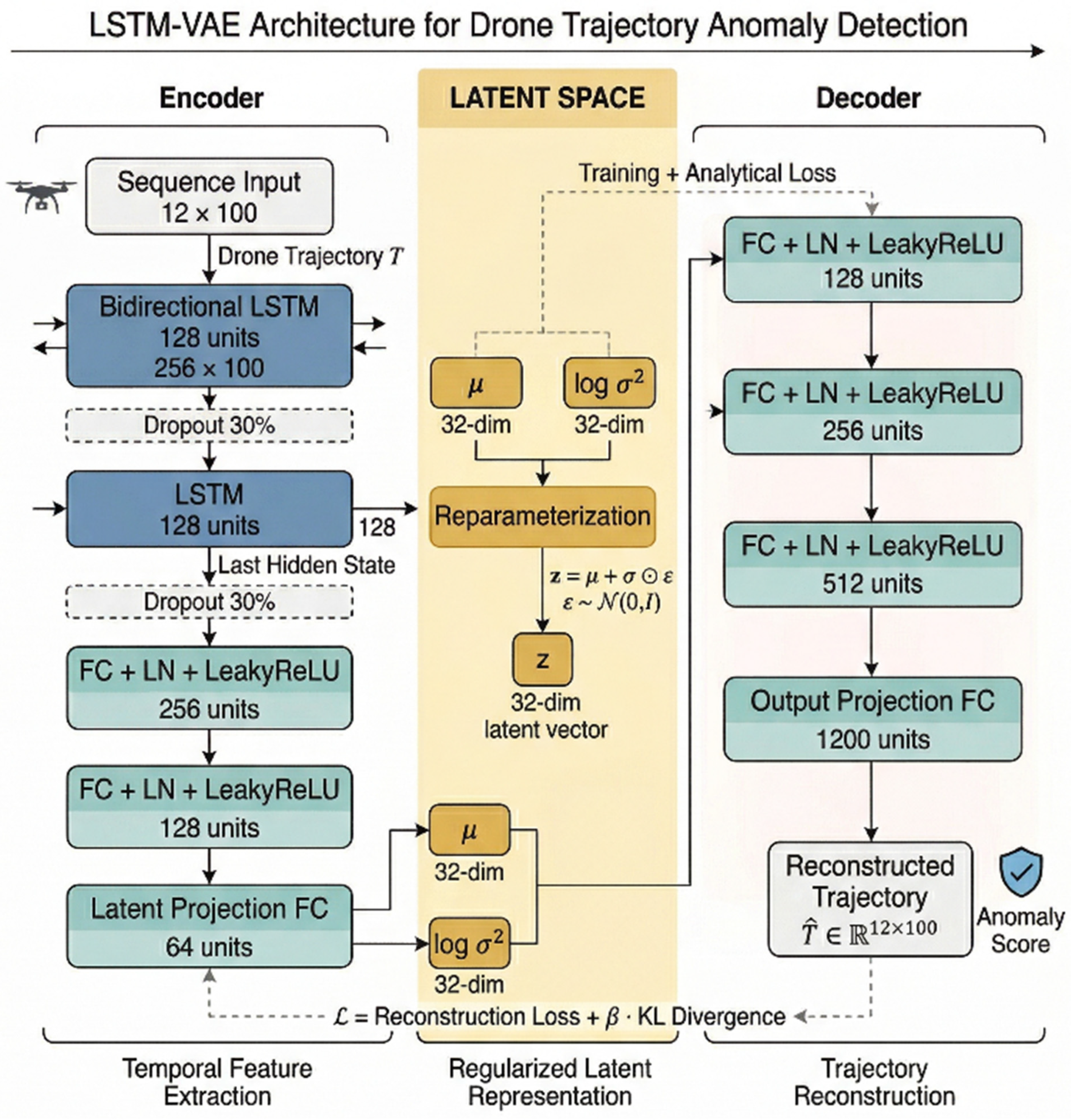
Our proposed LSTM-VAE architecture integrates bidirectional LSTM encoding with variational inference to acquire temporal representations of drone trajectories. The architecture has an encoder network that turns input sequences into latent distributions and a decoder network that turns latent samples into trajectories. The architecture is illustrated in Figure 1 below.
Encoder Architecture: The encoder takes the input sequence
T R L × F
and processes it through a series of fully connected and recurrent layers. The sequence input layer first takes in input with the shape
T R F × L , F × L = 12 × 100
which means that there are 12 features over 100 timesteps. The next step is to pass this sequence through a bidirectional LSTM layer with 128 units [24]. This layer processes the data in both directions to create hidden states that capture bidirectional temporal context. The output shape is (256 × 100). For regularization, a 30% dropout layer [33] is used. Then, a unidirectional LSTM layer with 128 units processes the sequence even more and only outputs the last hidden state as a fixed-length 128-dimensional representation. A dropout layer with an extra 30% helps to keep things regular. The resulting representation then goes through two fully connected layers: the first one has 256 units, and the second one has 128 units. Both use layer normalization [34] and LeakyReLU activation (α = 0.1). A final latent projection layer gives 2d = 64 values that stand for μ and log σ2 for a d = 32-dimensional latent space. The complete layer-by-layer encoder and decoder specification is summarized in Table 2.
Decoder Architecture: The decoder takes the latent sample
z N μ , diag σ 2
and builds the flattened trajectory
T ^ R L F
from it. A latent input layer takes in a latent vector with d = 32 dimensions. This vector is then passed through three fully connected layers, each with 128, 256, and 512 units, respectively. Each layer uses layer normalization and LeakyReLU activation. The last output projection layer maps to 1200 units, which creates the reconstructed flattened trajectory with dimensions
L   F = 100 × 12 = 1200

3.3. Training Objective

The model is trained to maximize the evidence lower bound (ELBO), which provides a tractable lower bound on the log-likelihood of the data:
L θ , ϕ ; T = E q z T log p T z β D K L q z T , p z
The first term represents the reconstruction likelihood, implemented as negative mean squared error between the input and reconstructed trajectory, it rewards the decoder for producing reconstructions close to the original. The second term is the Kullback–Leibler (KL) divergence, an information-theoretic measure of dissimilarity between two probability distributions defined as
D K L q p = E q log q p
which is zero when the distributions are identical and grows as they diverge. In our setting, this divergence is computed between the approximate posterior
q z T = N μ T , d i a g σ 2 T
and the standard normal prior
p z = N 0 , I
which has a closed-form solution for Gaussian distributions. The combined objective is known as the evidence lower bound (ELBO): maximizing it pushes the encoder to produce a latent posterior that is both informative for reconstruction (low MSE) and well-regularized toward a standard normal prior (low KL). The hyperparameter β balances these two goals, small β prioritizes reconstruction fidelity, large β prioritizes a smooth, well-organized latent space.
We employ β-VAE annealing [20] to prevent posterior collapse, a common failure mode where the model ignores the latent space and relies solely on the decoder. The annealing schedule linearly increases β from 0 to β_max = 0.5 over the first 40 epochs, allowing the model to first learn useful reconstructions before gradually enforcing latent space regularization.

3.4. Anomaly Scoring

At inference time, the anomaly score for a trajectory T is computed as the mean squared reconstruction error:
s T = 1 L · F i = 1 L · F T i T i ^ 2
Trajectories with scores exceeding a threshold τ are classified as anomalous. The threshold is determined from the validation set as the 95th percentile of reconstruction errors, ensuring that approximately 5% of normal trajectories would be flagged (corresponding to a 5% false positive rate on the validation distribution).

3.5. Baseline Methods

We compare our bidirectional LSTM-VAE to a unidirectional LSTM-VAE variant and four additional baselines that use different ways to find anomalies. Fully Connected VAE (FC-VAE): In this model, we use an encoder–decoder type architecture in which the input of the encoder and output of a decoder is on flattened trajectory vectors. The sizes of the encoder layers are 512, 256, 128, 64 respectively, and the decoder architecture is symmetric. This is a baseline to test whether the effect of the variational (rather than temporal) modeling per se is significant, or its temporal nature adds more appeal. Standard Autoencoder: This autoencoder has the same architecture as the last model but does not have the VAE part. Therefore, the second model disentangles the contribution of variational inference from the standard autoencoding. One-Class SVM (OC-SVM) OC-SVM is a standard method for one-class classification [35]. We use an RBF kernel and let the implementation automatically select a best scale, based on the median pairwise distances. OC-SVM learns a decision boundary from the normal data in kernel “space” that encloses the normal distribution according to a learned Laplacian ball, selecting points as anomalies outside of this boundary. Isolation Forest is an ensemble baseline, which uses 100 trees of approximately depth 64, which detect anomalies given recursively random partitioned decision trees. This method makes use of the characteristic that outlier points are few and different, therefore requiring few such random “splits” to detect them. In this method, we set the contamination parameter to 5%, so that it harmonizes with the behavior of most of the other methods (in terms of threshold selection).

3.6. Domain-Aware LSTM-VAE

The generic LSTM-VAE described in Section 3.2 treats trajectory features in their raw Cartesian-derived form and weights every timestep equally in the reconstruction loss. Neither choice reflects the operational structure of facility protection scenarios, where (a) anomaly is a function of relative position with respect to a known protected site, and (b) reconstruction fidelity at near-facility timesteps carries greater operational significance than fidelity at distant timesteps. We propose two architectural modifications that introduce these inductive biases without altering the encoder–decoder topology, layer dimensions, or hyperparameters of the baseline LSTM-VAE.
Polar Coordinate Input Representation: The 12 raw input features are replaced by 12 polar features expressed relative to the facility center—radial distance r, azimuth components sin θ and cos θ (decomposed to avoid the ±π wraparound discontinuity), altitude z, radial velocity ṙ, tangential velocity r θ . , vertical velocity ż, heading error angle (between velocity and the inward radial direction), speed magnitude, an inverse distance proximity score 1/(1 + r/r0), acceleration magnitude, and radial acceleration r .. . The feature count is preserved at 12 to ensure the encoder–decoder architecture remains identical to the baseline; only the geometric basis of the input changes. This representation makes facility-relative quantities first-class inputs rather than implicit features that the network must derive from absolute coordinates.
Distance-weighted reconstruction loss. The baseline reconstruction loss is the unweighted mean squared error
L recon = mean T ^ T 2
The domain-aware variant replaces it with a per-timestep distance-weighted form
L r e c o n D A = m e a n W T ^ T 2
where W t = 1 + α exp r t r 0 with α = 1.0 and r0 = 200 m. The per-timestep weight ranges from 1 (far from the facility) to 2 (at the facility center), allocating effective model capacity toward reconstructing trajectory segments that lie near the protected zone. The KL divergence term is unchanged. At inference, anomaly scores use the unweighted MSE, ensuring AUC-ROC values remain directly comparable to the baseline LSTM-VAE.
The two modifications together require no additional learnable parameters and preserve the baseline’s training schedule, latent dimension, and regularization configuration.


4. Experimental Setup

4.1. Simulation Environment

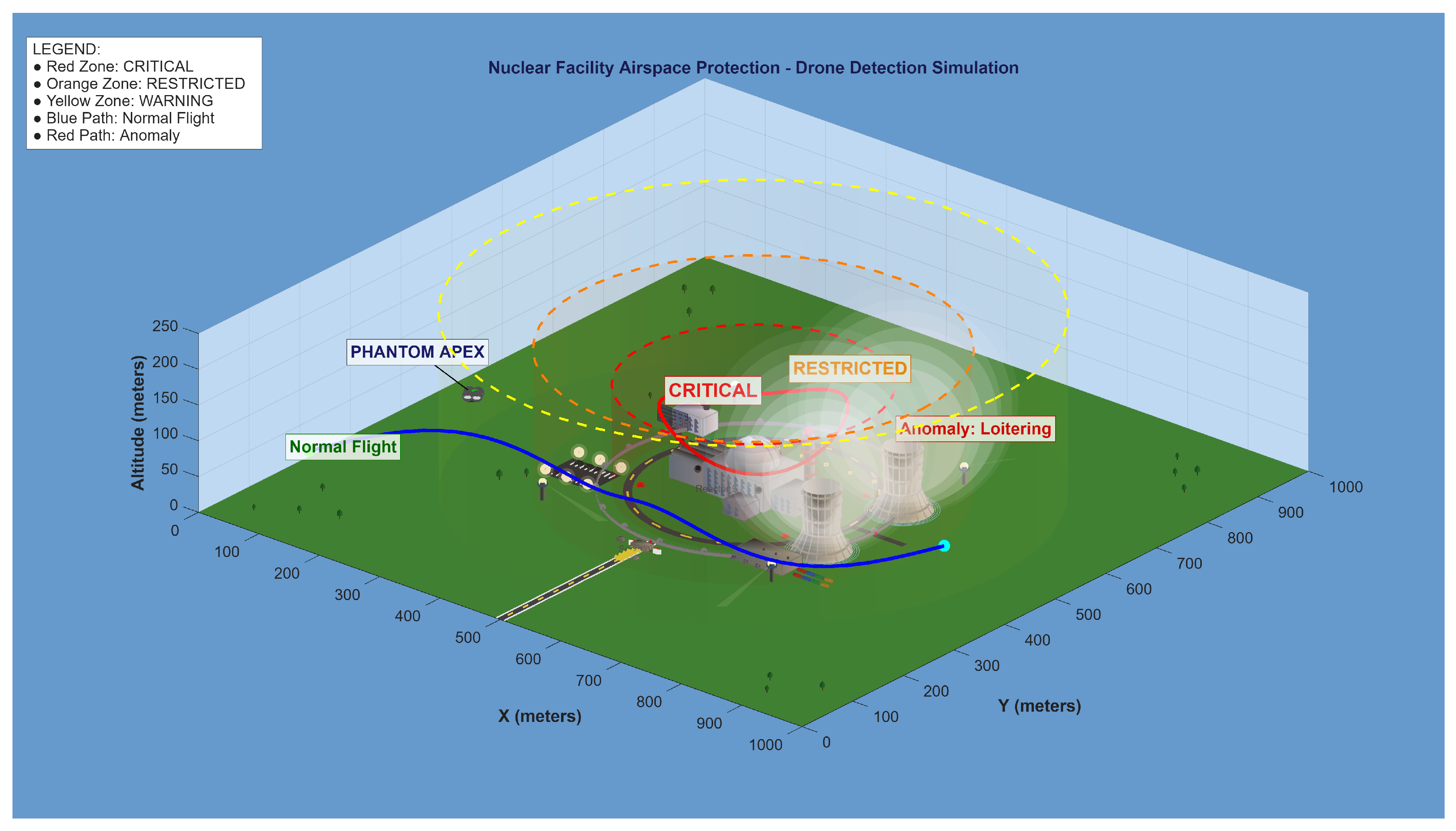
We set up a realistic simulated nuclear facility protection scenario, highlighted in Figure 2 to collect realistic drone trajectories for training and evaluation.

Environment Parameters:

The simulation environment comprises a 1000 m × 1000 m horizontal arena with altitudes from 0 to 250 m above ground level. All the simulation takes place within this area with the protected facility situated at the center of the arena at (500, 500), m. There are three zones around the facility, a critical one to a radius of 180 m representing the outer perimeter of the facility and highest level of threat, a restricted zone at radius of 280 m where entering controlled airspace requires permission, and a warning zone outside where legitimate traffic is expected and airspace is monitored.

4.2. Trajectory Generation

We generated a diverse dataset of 2500 drone trajectories encompassing both normal operations and anomalous intrusion attempts; the full class breakdown is given in Table 3. Each trajectory consists of 100 sequential observations sampled at 1 Hz, corresponding to approximately 100 s of flight time. This is a sufficient amount of time to sample complete behavioral patterns while remaining computationally tractable. Although the simulator generates labeled normal and anomalous trajectories, the anomaly detector is trained exclusively on the normal class and never observes anomaly labels during training; it learns a statistical envelope of normal behavior rather than a deterministic rule that distinguishes anomaly classes. The simulation provides a controlled environment for ranking detection methods under matched conditions; the hard anomaly evaluation in Section 5.7 further probes generalization to threat profiles outside the training distribution support. The following parameters are used to generate simulated trajectories: stochastic flight dynamics with speed bounded to 0–20 m/s, altitude bounded to 0–250 m, smooth heading transitions subject to a turning rate limit, and additive Gaussian wind perturbations and GPS position uncertainty. These parameters are designed to match publicly available drone flight specifications and FAA operational guidelines for small UAS. Though simulated data cannot recreate all of the difficult characteristics of real data such as sensor noise, environmental variability, and adversarial adaptation, they do provide a limited environment suitable for systematic evaluation of detection methods under similar conditions. Validation of real-world datasets such as ADS-B flight datatypes on OpenSky Network or operational UAV flight logs is an important direction of future work.
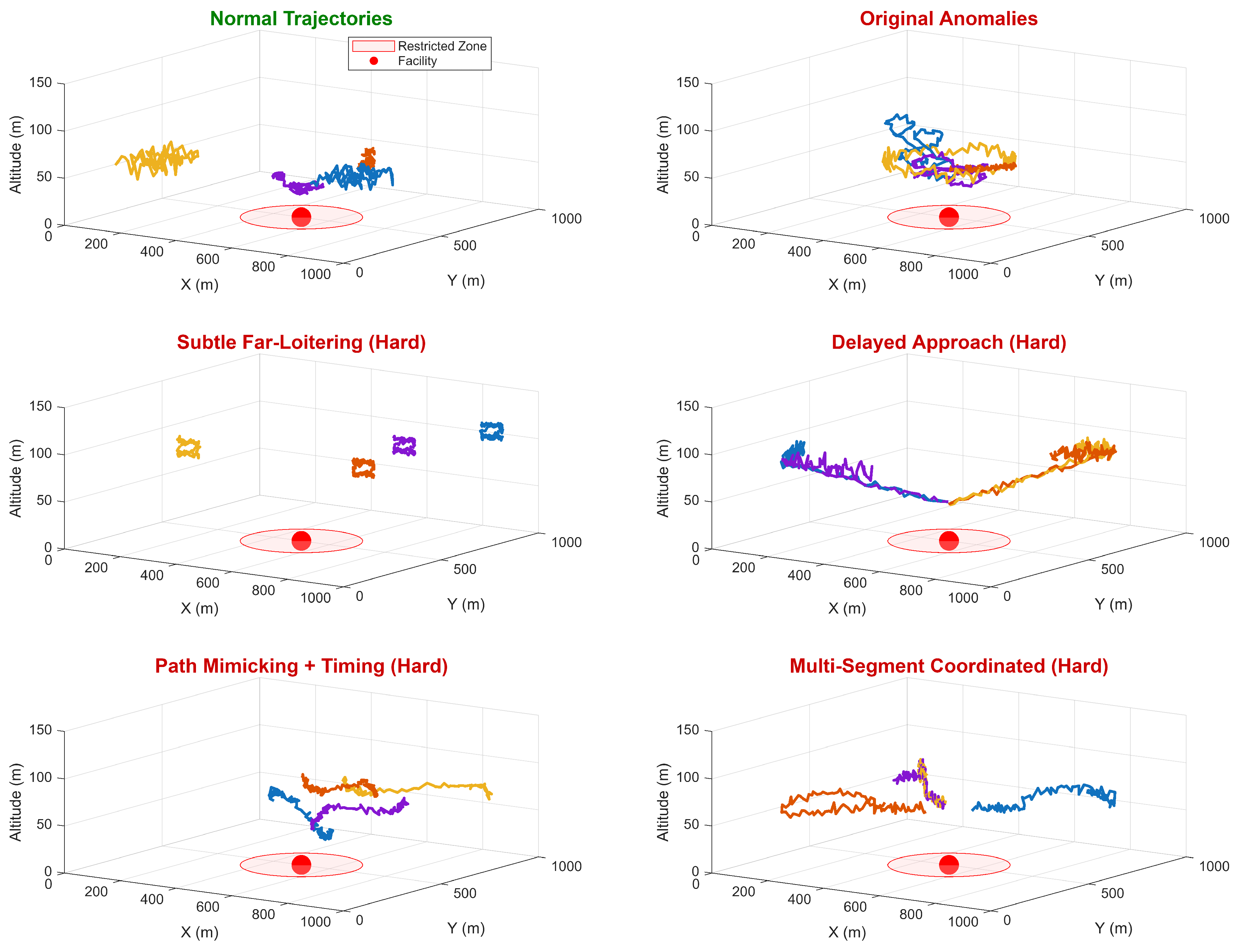
Normal trajectories suggest that everything is safe and that the drones are at a safe distance from the protected facility, the largest class being delivery trajectories (40%, 800 total). Delivery trajectories connect two random locations outside the warning zone in efficient, direct routes with slight deviations, as might be caused by wind and course correction at heights of 50 to 100 m. Survey trajectories (35%, 700) follow the constant regular grid patterns typical in surveying, mapping, inspection, and even farming. They turn at regular intervals and climb or descend while avoiding the restricted area of airspace. The last group of normal trajectories represent recreational flight (25%, 500). Their irregularities in the rate of changes in speed, course directions are more reminiscent of a hobbyist having fun with his drone than those in a delivery, but still light years away from the restricted airspace. Anomalous trajectories simulate different threat scenarios that break the rules of flying in the airspace and show dubious behavior patterns. Loitering trajectories (30%, 150) consist of circular and figure-eight flight patterns in and around the restricted area, similar to surveillance missions to gather intelligence on the activities of the facility. Direct approach trajectories (25%, 125) show straight-line flight patterns toward the center of the restricted area, possibly simulating attempts to drop off supplies or even attacking the facility. Evasive trajectories (25%, 125) show zigzag patterns with quick turns in direction, similar to trying to evade detection and approaching the restricted area. Finally, surveillance trajectories (20%, 100) show slow and deliberate flight patterns around the restricted area at a consistent distance from the facility while surveying different parts of the restricted area.
To assess robustness against threat profiles outside this initial taxonomy, we additionally constructed an augmented “hard anomaly” test set comprising four further classes designed to probe limitations of behavioral detection: (i) subtle far-loitering at the warning-zone boundary, (ii) delayed approach with extended dwell time before the restricted-zone breach, (iii) path mimicking, in which an anomalous trajectory replicates the spatial profile of a normal flight but at altered timing, and (iv) multi-segment coordinated approaches that distribute the threat across temporally separated maneuvers. Representative samples of all four hard anomaly classes are shown in the lower two rows of Figure 3. The hard anomaly set is used exclusively for evaluation; no model is trained on it. We acknowledge that this taxonomy remains non-exhaustive, real-world threat behaviors include hovering, dive maneuvers, formation flight, payload dropping, and sudden power-off crashes [36], and the open-ended nature of adversarial threat space is itself a limitation discussed in Section 6.4.

4.3. Data Partitioning

The dataset was split up according to standard machine learning methods, while still keeping the one-class classification model. The training set has 1500 normal trajectories that are only used to train the model. There are no unusual examples in the set, which is similar to how it is in the real world, where it is rare to have complete coverage of all threat types. There was a validation set of 300 normal trajectories that was used for hyperparameter tuning, choosing the threshold, and making early stopping decisions. The detection threshold was set at the 95th percentile of validation reconstruction errors. The rest of the data is the test set, which contains 200 normal and 500 anomalous trajectories (700 total) used for final evaluation. The 2:5 normal-to-anomalous ratio in the test set is a deliberate choice for accurate metric estimation: AUC-ROC is invariant to class balance, and a higher anomaly count tightens the variance of precision and recall estimates at any chosen threshold. We emphasize that this ratio reflects the evaluation set composition, not an assumption about deployment time prevalence. Real security operations exhibit anomaly rates well below 1%, and a separate deployment-realistic evaluation under that regime is presented in Section 5.8.

4.4. Preprocessing

To avoid data leakage, features were normalized using z-score standardization, and statistics were only calculated from the training set:
x n o r m a l i z e d = x μ t r a i n max σ t r a i n , 0.01
A minimum standard deviation of 0.01 stops division by zero for features that are almost constant. To deal with extreme outliers while keeping most of the distributional information, normalized values were clipped to ±10 standard deviations.

4.5. Training Configuration

For fairness in comparison, we trained all deep learning models (LSTM-VAE, FC-VAE, autoencoder) on the same training set of 1500 normal trajectories with the same hyperparameters, optimizer settings, and learning rate schedules. Models were not tuned for hyperparameters specific to model architecture, but the same hyperparameters were used across all networks. For classical methods, OC-SVM and Isolation Forest, we used automatic kernel scale selection based on median pairwise distances and 100 trees with 5% contamination, respectively, which are both standard defaults that require no hyperparameter tuning. Hyperparameter choices follow established practice in the VAE literature and were validated through preliminary experiments. A latent dimension of 32 provides sufficient capacity to encode 12-dimensional features over 100 timesteps without overparameterizing the latent space. Learning rate of 0.0008 with step decay was decided on grid search over {0.0001, 0.0005, 0.0008, 0.001} on validation loss. Β maximum of 0.5 follows guidance from the β-VAE literature [20] for anomaly detection tasks, providing a trade-off between reconstruction accuracy and regularization of the latent space. The 40-epoch warmup period mitigates posterior collapse by letting the model first learn useful reconstructions. The 0.3 dropout ratio is the standard rate for regularization for sequence models. Training was conducted on an NVIDIA GeForce RTX 4070 Ti GPU with 12GB of memory and all models were trained for the full 150 epochs to ensure fair comparison of final converged performance. To ensure reproducibility under deterministic seeding, both the CPU random number generator (rng(seed) in MATLAB R2025b version) and the GPU random number generator (gpurng(seed)) were initialized at the start of each run; we observed that omitting the GPU seed leaves operations such as the variational reparameterization sampler and dropout governed by an unseeded GPU stream, producing substantial run-to-run variance even at fixed CPU seed. All reported results in Table 4 are mean ± standard deviation over five seeds (42, 123, 456, 789, 2024), with both CPU and GPU streams seeded identically per run. The shared training configuration is summarized in Table 5.

4.6. Evaluation Metrics

We use a number of different metrics to judge how well the model works. AUC-ROC (Area Under the Receiver Operating Characteristic Curve) [38] measures how well a model can tell the difference between two things at any threshold. The values range from 0.5 (random) to 1.0 (perfect discrimination). The F1-score is the harmonic means of precision and recall at the chosen operating threshold. It balances the rate of false positives and false negatives. Precision is the measure of the actual number of true positive anomalies identified. Precision is particularly significant in security-related applications where precision must be high to maintain the trust of operators. The measure of actual identified anomalies is called recall; it is also known as sensitivity or true positive rate. Finally, we report the accuracy of classification; however, it should be noted that it might be misleading if not considered on well-balanced test sets.

5. Experimental Results

5.1. Overall Performance Comparison

Table 4 shows the full multi-seed benchmark results for all seven methods. The domain-aware LSTM-VAE achieves the highest AUC-ROC at 0.9617 ± 0.0071, while the three generic VAE variants cluster near 0.92 and the three non-VAE baselines cluster near 0.77.
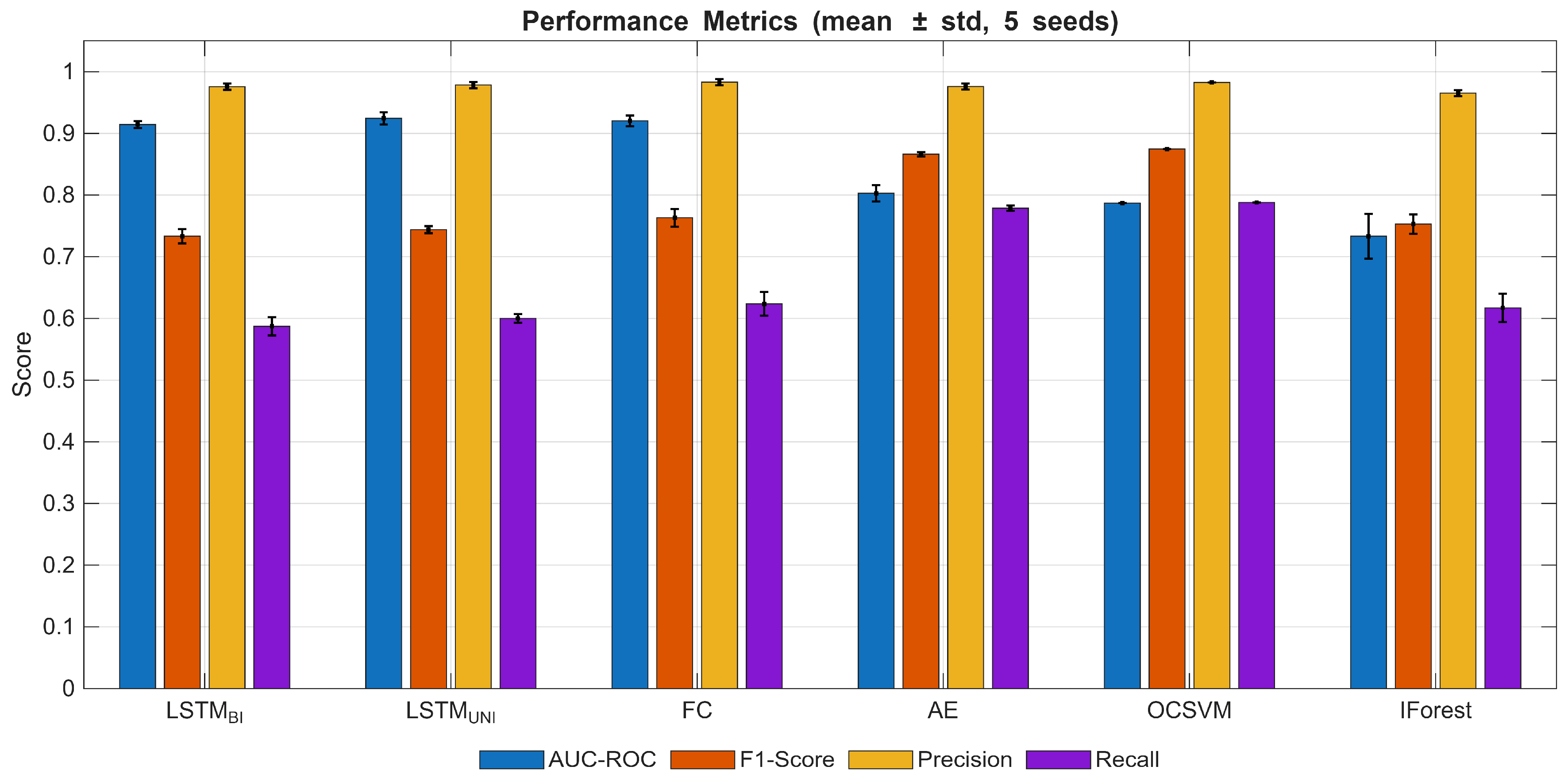
Table 4 shows the multi-seed benchmark of all seven methods. The three VAE variants, bidirectional LSTM-VAE, unidirectional LSTM-VAE, and fully connected VAE, cluster within standard deviation of one another at AUC-ROC ≈ 0.92, while the three non-VAE baselines (standard autoencoder, One-Class SVM, Isolation Forest) cluster around AUC ≈ 0.77. The performance gap between these two groups, approximately 15 percentage points, is well outside the seed-to-seed standard deviation of any individual method. The domain-aware LSTM-VAE described in Section 3.6 outperforms all generic methods, achieving 0.962 ± 0.007, a 3.7 percentage-point gain over the best generic VAE variant at no additional parameter cost. All methods maintain high accuracy (>96%) at the 95th-percentile validation threshold, reflecting the conservative operating point. Precision varies more substantially across methods (0.59 to 0.79), with the domain-aware variant achieving 0.745. Recall is the dimension on which methods most differ; the domain-aware variant achieves the strongest recall at this operating point.

5.2. ROC Curve Analysis

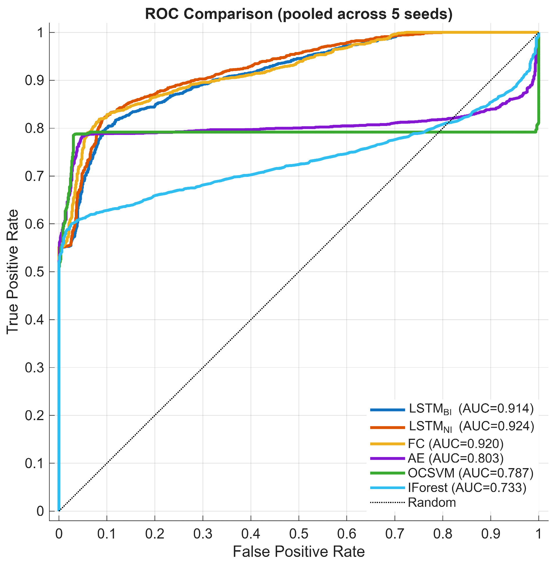
Figure 4 shows the Receiver Operating Characteristic (ROC) curves [38] for the six benchmark methods; the domain-aware variant is shown separately in Section 5.7. These curves show the balance between the true positive rate and the false positive rate at different detection thresholds.
The ROC analysis supports several conclusions. The three VAE variants (bidirectional LSTM-VAE, unidirectional LSTM-VAE, FC-VAE) trace closely overlapping curves throughout the operating range, while the three non-VAE baselines (standard autoencoder, OC-SVM, Isolation Forest) sit substantially below. This separation is most pronounced in the low-FPR regime (FPR < 0.2), which is the operating region of primary concern for security applications where false alarms carry direct operational cost. At a 5% false positive rate, the VAE variants achieve approximately 70% true positive rate, compared to roughly 55–60% for the non-VAE baselines, a gap consistent with the AUC-ROC ranking in Table 4.

5.3. Performance Metrics Visualization

Figure 5 shows all of the evaluation metrics for each method side by side, making it easy to see how their strengths and weaknesses compare.

5.4. Reconstruction Error Distributions

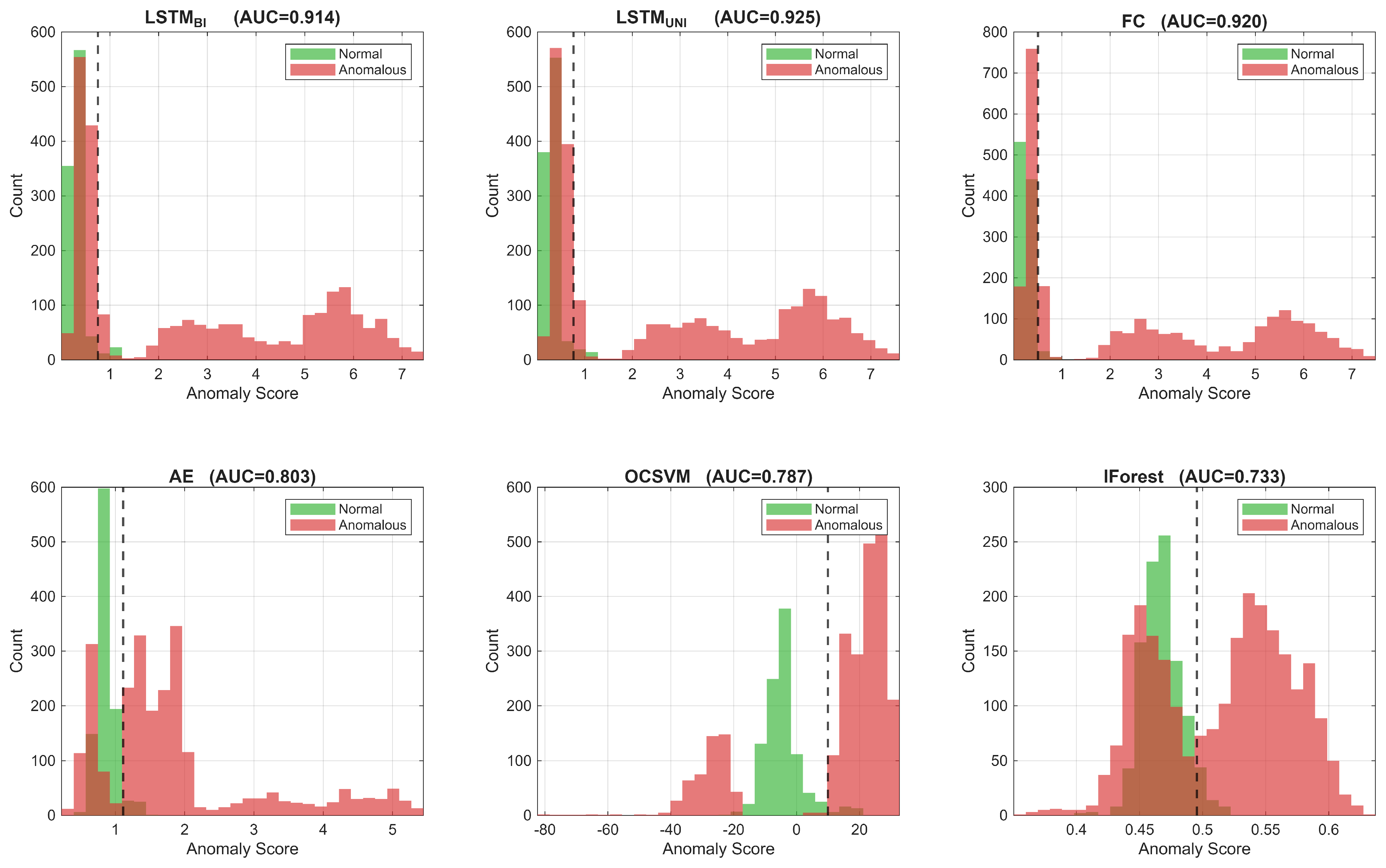
Figure 6 shows the reconstruction error distributions for normal and anomalous test trajectories across the six benchmark methods. The greater the separation between the two distributions, the higher the AUC; the position of the 95th-percentile validation threshold relative to each distribution further indicates the operating point sensitivity of each method.
The three VAE methods produce the most distinct bimodal distributions, with anomalous trajectories systematically reconstructed less accurately than normal ones. The overlap of the two distributions is smaller for the VAE variants compared to the non-variational baselines, consistent with the AUC-ROC ranking in Table 4. The standard autoencoder shows substantial overlap consistent with its lower AUC, although its F1-score remains competitive at the chosen threshold due to the operating point sensitivity discussed above.

5.5. Latent Space Analysis

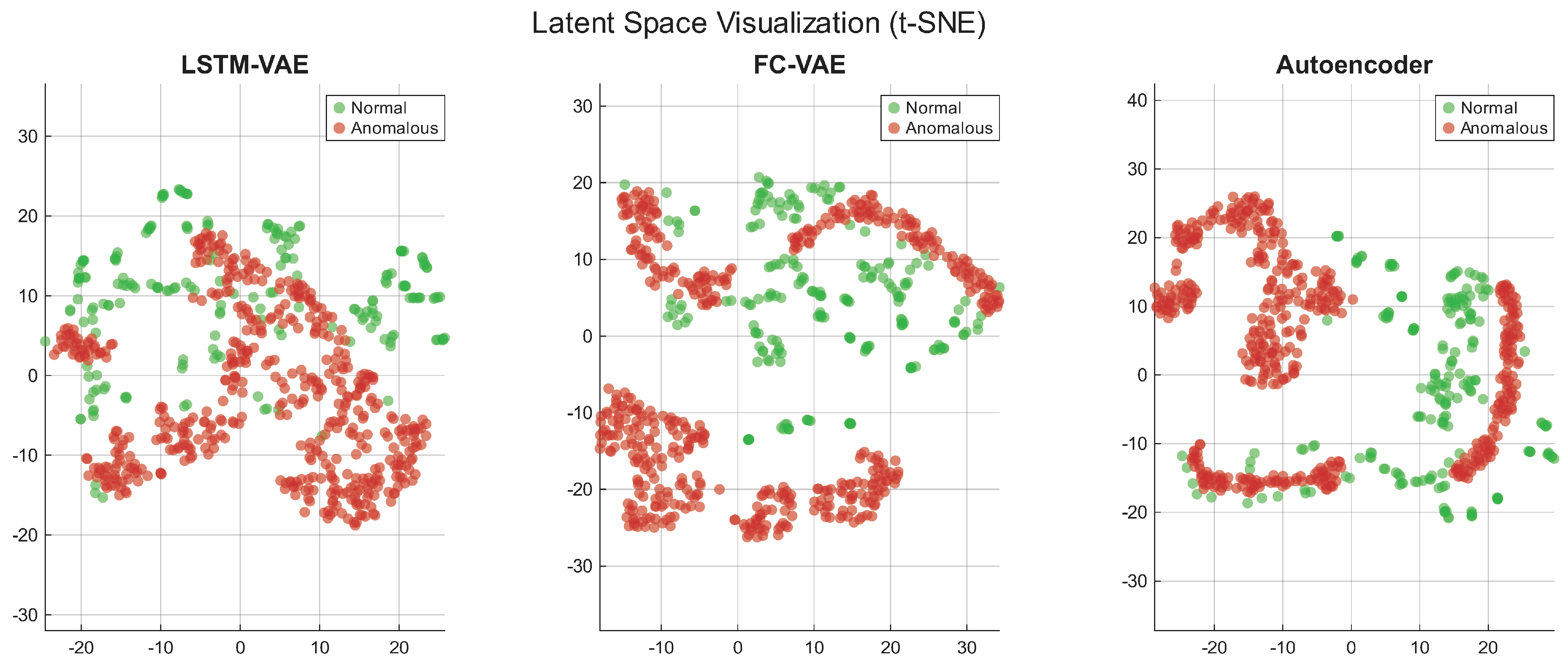
To examine the latent geometry learned by each deep model, we visualize the learned representations using t-SNE (t-distributed stochastic neighbor embedding) [39] for dimensionality reduction. Figure 7 shows the latent spaces learned by LSTM-VAE, FC-VAE, and the standard autoencoder.
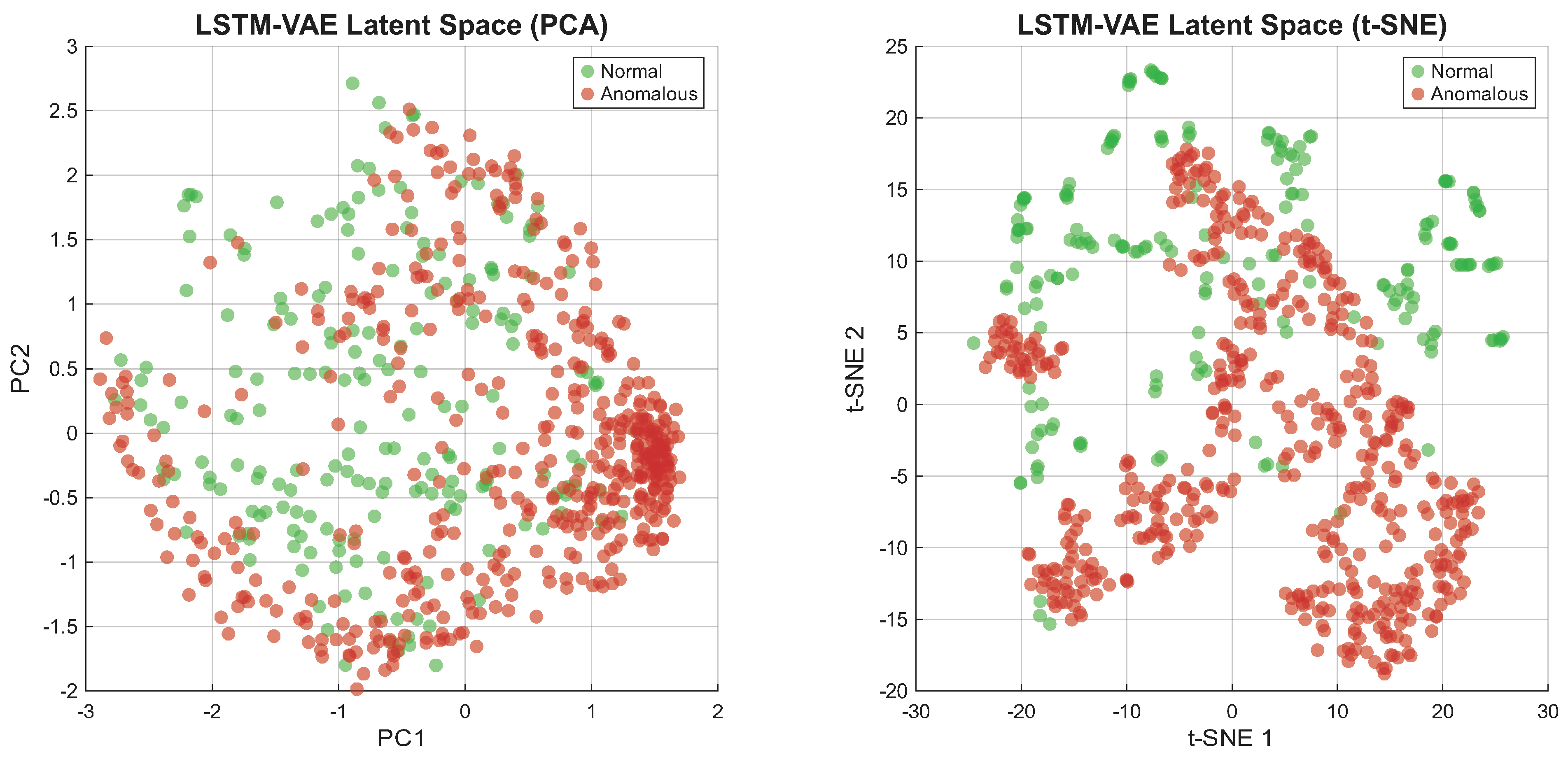
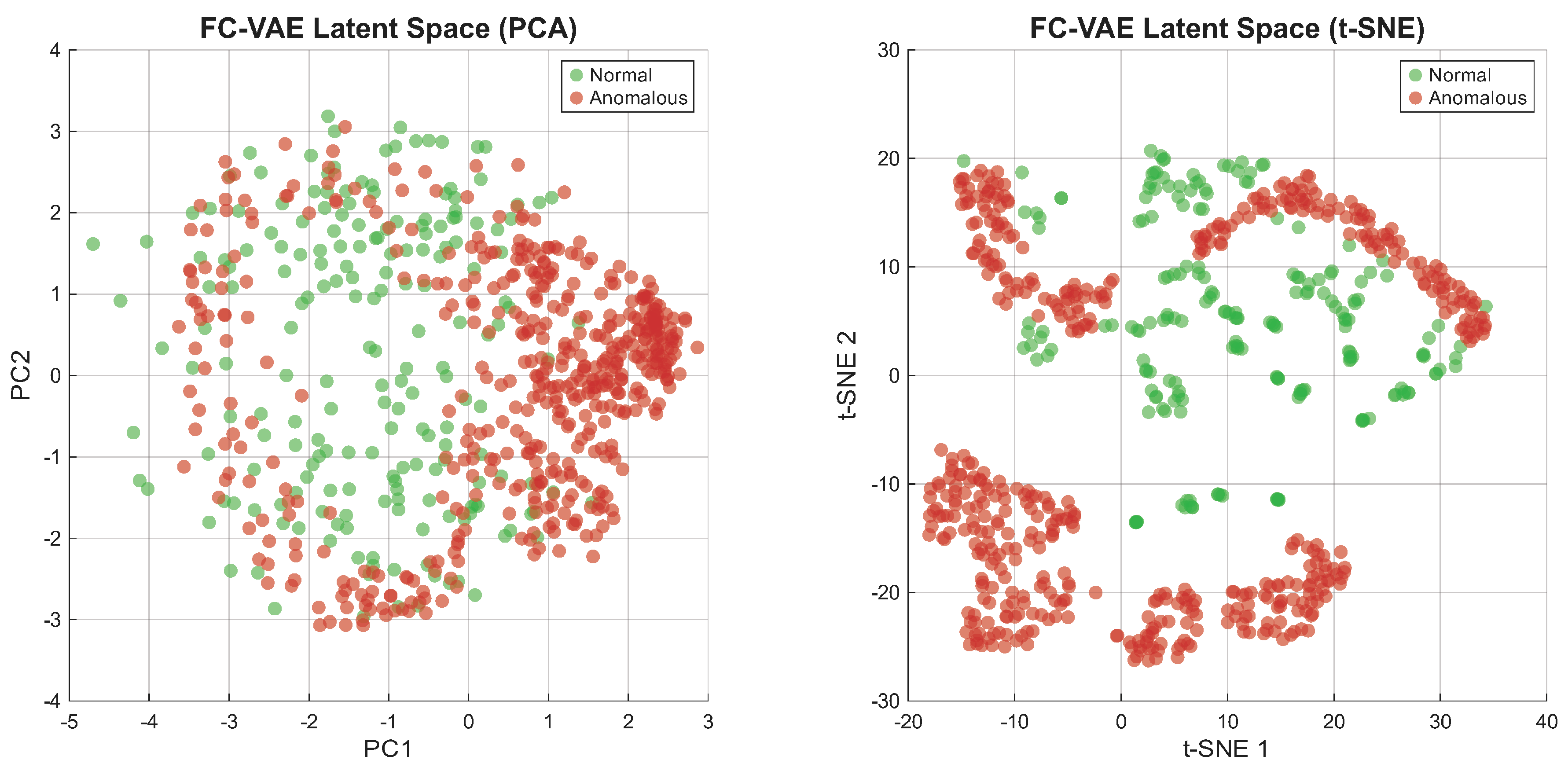
The two VAE latent spaces (LSTM-VAE and FC-VAE) exhibit comparable separation between normal and anomalous clusters, both substantially cleaner than the standard autoencoder. Normal trajectories occupy relatively tight distributions while anomalous trajectories are displaced into distinct regions of the space, consistent with the variational regularizer organizing the latent geometry such that out-of-distribution inputs are systematically displaced rather than the separation arising purely from reconstruction error. The LSTM-VAE latent space is examined in detail in Figure 8, with the corresponding FC-VAE latent space shown in Figure 9.

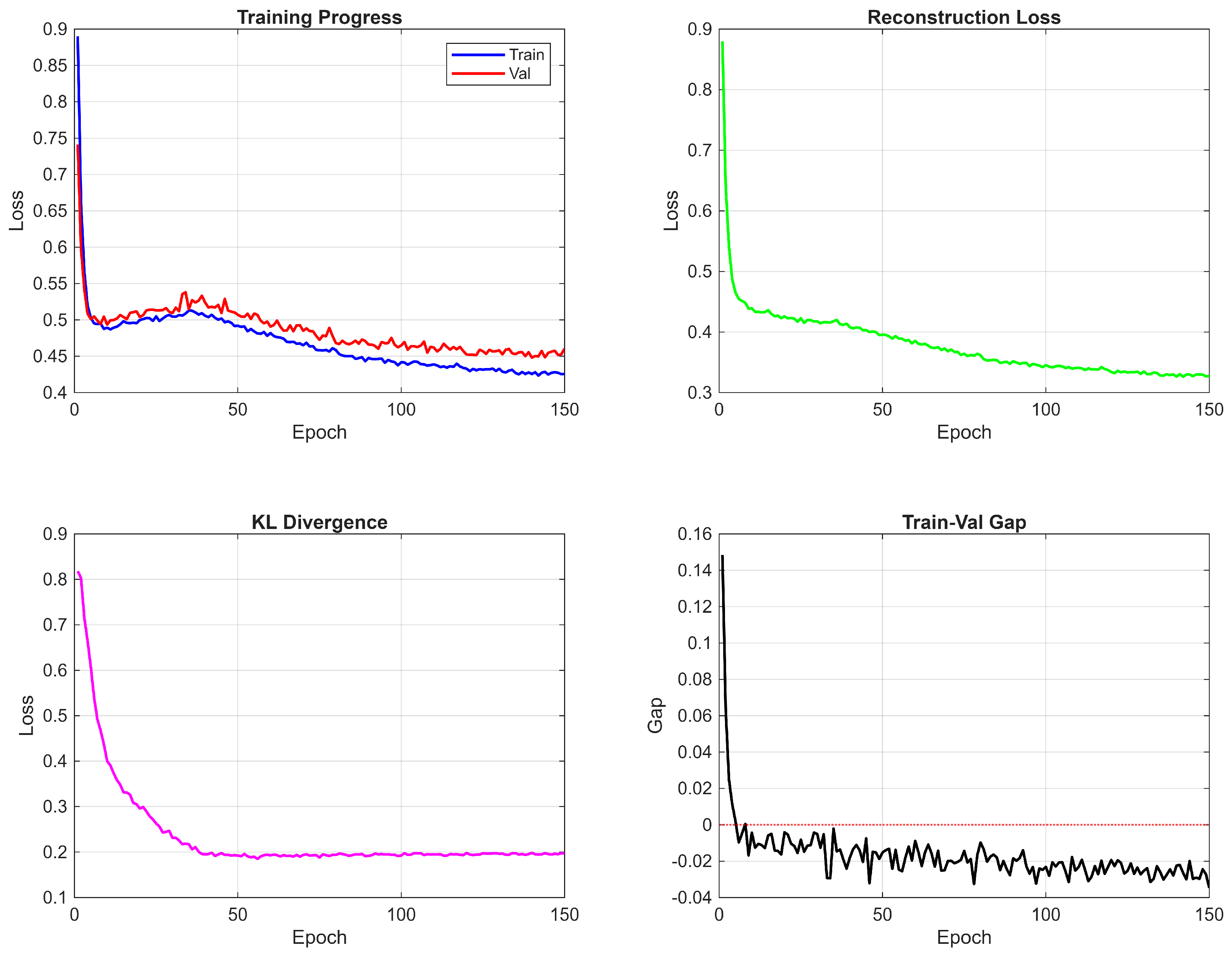
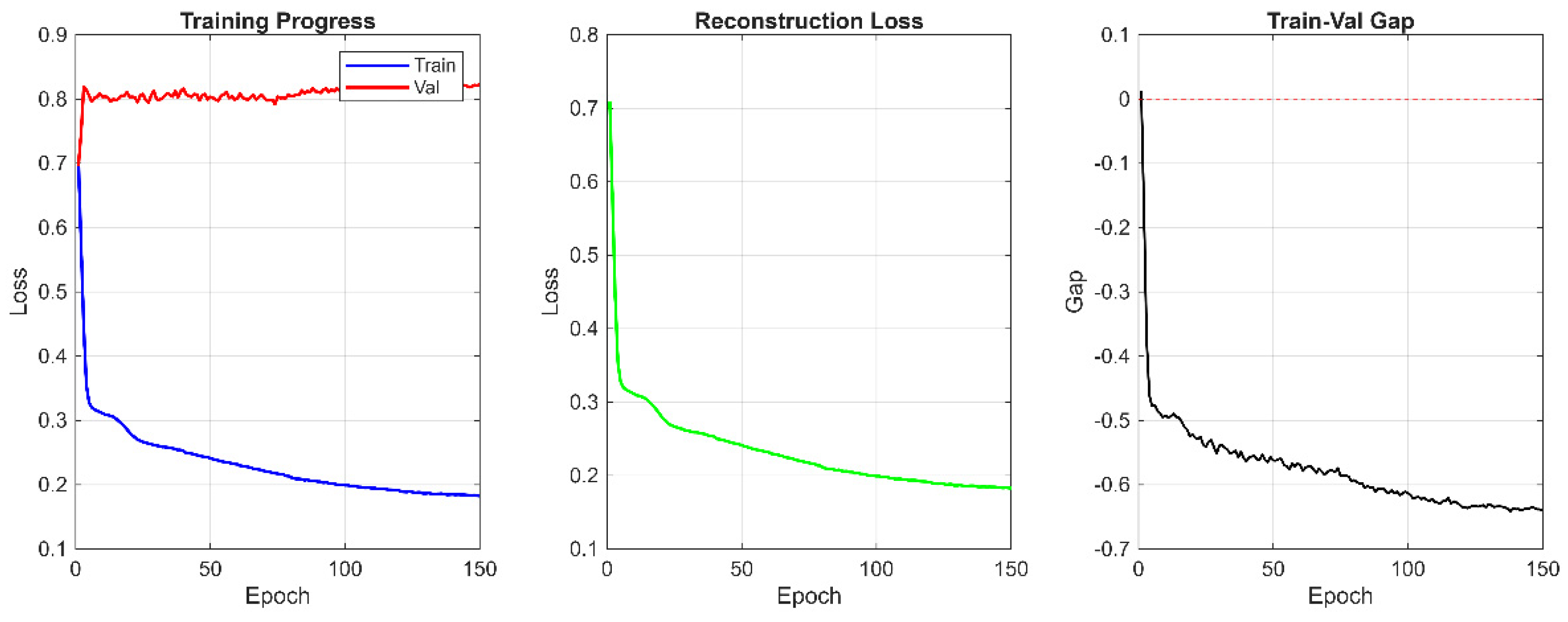
5.6. Training Dynamics

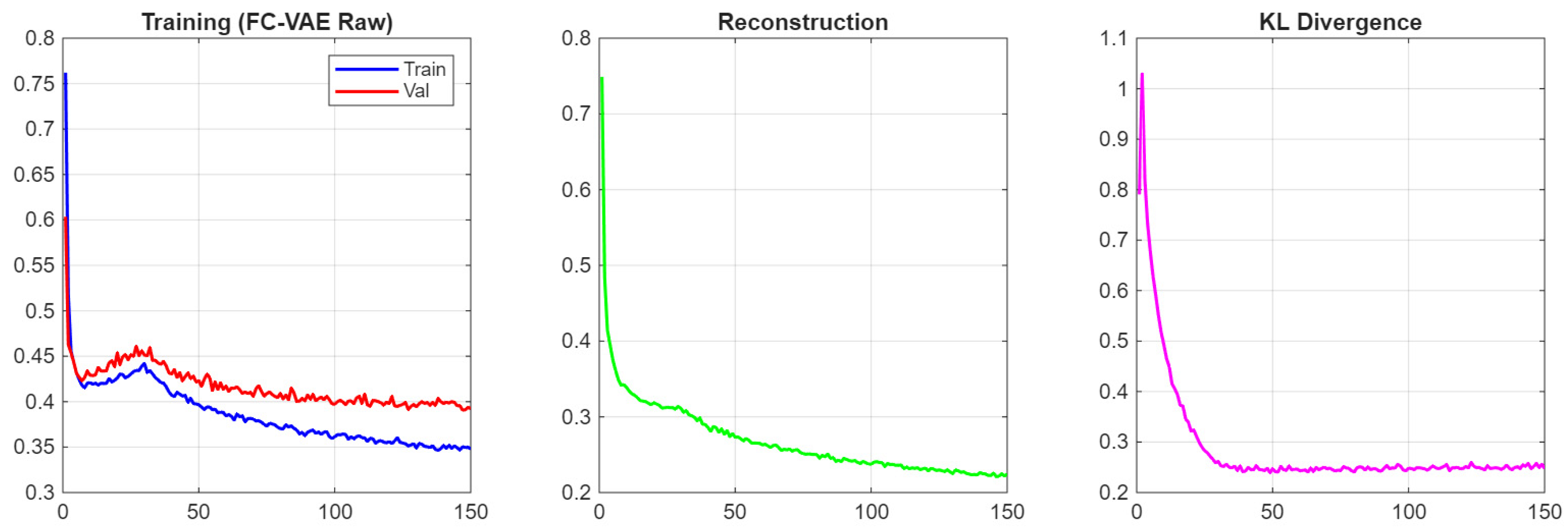
Figure 10, Figure 11 and Figure 12 present the training curves for LSTM-VAE, FC-VAE, and the standard autoencoder, showing the evolution of loss components over 150 epochs.
The training curves show that all the models fully converge. We see KL divergence in LSTM-VAE go up during β warmup and converge as the model learns to strike a balance between reconstruction and regularization. The gap between training set losses and validation set losses is small throughout training so we are not overfitting very much. FC-VAE converges faster than the LSTM variants but reaches a comparable final loss and AUC (Table 4), consistent with variational regularization rather than encoder type driving anomaly detection performance in this domain.

5.7. Domain-Aware Results

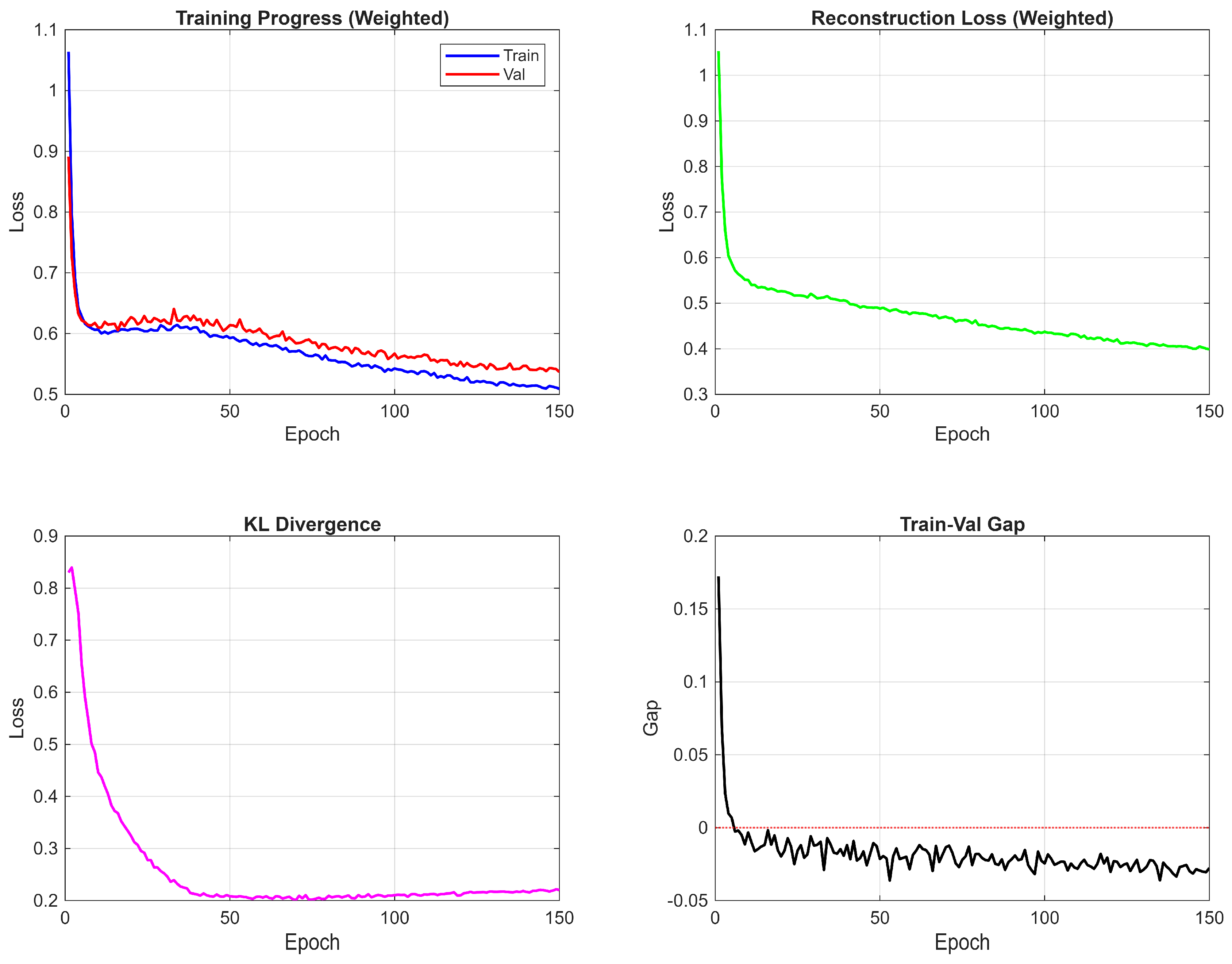
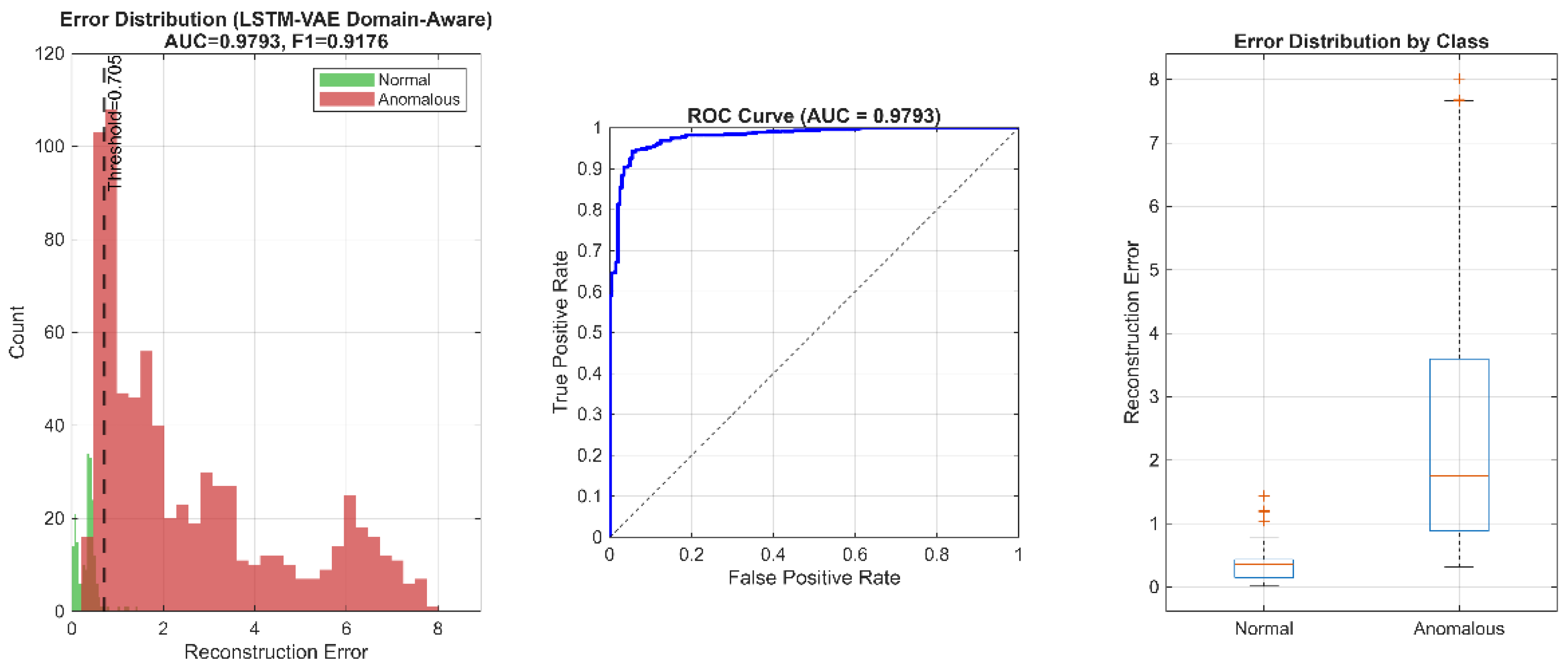
The domain-aware LSTM-VAE introduced in Section 3.6 was trained and evaluated under the same multi-seed protocol as the generic VAE methods, on both the original and the augmented hard anomaly test sets. Figure 13 shows the training dynamics; Figure 14 shows the resulting score distribution, ROC curve, and per-class score boxplot on the hard anomaly test set. Across five random seeds, the domain-aware variant achieves AUC-ROC of 0.962 ± 0.007 on the original test set and 0.973 ± 0.005 on the hard anomaly test set, a 3 to 4 percentage-point improvement over the best generic VAE method (Table 4) at no additional learnable parameter cost. The improvement is consistent across seeds and is larger on the hard anomaly set than on the original, indicating that the polar representation and distance-weighted loss generalize beyond the original anomaly taxonomy rather than overfitting to it.

5.8. Deployment-Realistic Evaluation

Deployment of an anomaly detector at a critical infrastructure facility encounters anomaly rates orders of magnitude lower than the 2:5 ratio used for metric estimation in Section 5.1. To assess detection performance under deployment-realistic conditions, we performed a bootstrap evaluation in which test batches were resampled at a 99:1 normal-to-anomalous ratio, repeated for 1000 iterations on each of the original and hard anomaly datasets. We report precision at constrained false positive rate operating points (P@1%FPR, P@5%FPR, P@10%FPR), which directly characterize alarm quality at the low-FPR regimes relevant for security deployment. Table 6 summarizes the results. The variational methods (LSTM-VAE BiLSTM, LSTM-VAE unidirectional, FC-VAE) cluster tightly together and improve under the harder threat distribution, while the non-variational baselines either remain flat or degrade. This pattern is consistent with our finding in Section 5.1 that variational regularization, rather than bidirectionality or LSTM-specific encoding, is the dominant performance driver in this domain.
The domain-aware variant achieves the highest P@5%FPR and P@10%FPR on both datasets, indicating that its precision advantage holds under deployment-realistic class imbalance at operationally relevant low-FPR points.

6. Discussion

6.1. The Value of Temporal Modeling

The multi-seed benchmark in Section 5.1 isolates a clear finding: the bidirectional LSTM-VAE (0.9145 ± 0.0055), unidirectional LSTM-VAE (0.9245 ± 0.0099), and fully connected VAE (0.9203 ± 0.0085) achieve statistically indistinguishable AUC, while the non-variational baselines, standard autoencoder (0.8029 ± 0.0133), One-Class SVM (0.7870 ± 0.0000), and Isolation Forest (0.7332 ± 0.0364), cluster roughly 15 percentage points lower. The performance gap is therefore attributable to variational regularization (the KL divergence term) rather than to bidirectional context or LSTM-specific temporal encoding. A plausible interpretation is that the violations defining anomaly in this domain—proximity to the facility, restricted-zone breach, and persistent boundary dwell—are largely expressible from the spatial distribution of trajectory points, so the smooth latent manifold imposed by variational regularization, on top of any sufficient encoder, captures the signal that distinguishes nominal from anomalous flight. Because all three VAE variants use identical raw trajectory features, the near-equivalence across recurrent and fully connected encoders is directly attributable to the variational regularizer, and motivates the domain-aware modifications introduced in Section 3.6, which target spatial structure (polar representation) and operational priority (distance-weighted loss) rather than temporal context.

6.2. Precision–Recall Trade-Offs in Security Applications

All methods achieve high accuracy (>96%) at the conservative 95th-percentile threshold, but precision varies substantially across methods (Table 4), making precision at low FPR (Section 5.8) the more discriminating operating metric. This operating point reflects the asymmetric cost structure of security applications, where false alarms erode operator trust while missed detections impose direct security risk. The domain-aware LSTM-VAE achieves 98.36% accuracy and 74.5% precision at this threshold, balancing alarm reliability against detection coverage. A system producing excessive false alarms will be ignored or disabled, rendering it operationally useless, so high precision at low FPR (as characterized in Section 5.8) is the dominant deployment constraint. Trajectory analysis is intended as one component of a layered security system, complementing physical modality detectors (radar, RF, acoustic, visual) that may catch threats invisible to behavioral analysis and vice versa. Where operational requirements call for higher recall, the threshold can be lowered to increase sensitivity; the domain-aware LSTM-VAE retains a precision advantage over the non-VAE baselines across the low-FPR operating range characterized in Section 5.8, providing operators flexibility to tune the trade-off without sacrificing alarm reliability relative to classical methods.

6.3. Comparison with Classical Methods

The classical baselines underperform the VAE family by a substantial margin. Isolation Forest achieves AUC of 0.7332 ± 0.0364 and One-Class SVM achieves 0.7870 ± 0.0000, both well below the ≈0.92 cluster of the VAE variants. Isolation Forest’s random partitioning approach can isolate outliers without learned representations but evidently fails to capture the structural regularities of nominal trajectories that the variational latent space encodes. OC-SVM likely suffers from the curse of dimensionality in the 1200-dimensional flattened trajectory space: kernel methods struggle to place effective decision boundaries in such high-dimensional input spaces, and the RBF kernel’s isotropic similarity assumption is poorly matched to the geometric structure of trajectory data.

6.4. Limitations and Future Work

Our study has some limitations which direct us to future work in this space:
Simulated Data and Threat Taxonomy: Our trajectories were generated through simulation rather than collected from real drone flights, and our anomaly taxonomy, eight behavior classes between the original and augmented sets, does not span the full space of operationally realistic threats. Hovering, dive maneuvers, formation flight, payload drop maneuvers, and sudden power-off crashes are all plausible threat profiles that lie outside our generative model. Sensor and environmental factors (GPS noise, wind variability, operational diversity, hardware faults) are also represented only schematically. Validation on real-world datasets such as ADS-B traffic from the OpenSky Network and operational UAV flight logs is the natural next step. Recent studies looking at adversarial attacks against DNN based ADS-B anomaly detection models [19] also show the necessity to evaluate the robustness of detection systems against intentional evasion, which we are not addressing here.
Class Imbalance and Operating Condition Variability: Our deployment-realistic evaluation in Section 5.8 addresses class imbalance through bootstrap resampling at a 99:1 ratio, but the class imbalance and domain-shift literature offers more sophisticated alternatives including class-aware adversarial adaptation, multi-source domain alignment, and soft selection decision fusion strategies recently demonstrated for fault diagnosis under variable operating conditions [36]. Adapting class-imbalance-aware techniques such as JCAN’s class-aware mechanism and joint domain alignment strategy to drone trajectory anomaly detection, where operating conditions vary across facility types, weather, and threat profiles, is a promising direction for future work.
Single Facility Scenario: We looked at how to protect a nuclear facility in one scenario. airports, nuclear plants, power plants and government buildings all present critical infrastructure which may have their own distinct nominal and anomalous flight patterns. Transfer learning methods may benefit trained models in one scenario, being useful in other scenarios also. Fixed Trajectory Length: Our architecture requires that input sequences always be of the same length. In the real world, deployment may have trajectories that last for differing amounts of time. Attention mechanisms or sequence-to-sequence architectures may be able to assist in entering variable length inputs.
Interpretability: As mentioned, the LSTM-VAE appears to detect anomalies well, but does a poor job of explaining why a certain trajectory is flagged abnormal. Attention mechanisms can support operator decision-making by surfacing which timesteps contribute most to the anomaly score, providing per-flight evidence for any flagged trajectory. Recent work on Transformer/VAE architectures [32] indicate self-attention may provide potential for temporal anomaly detection and may be adapted to our drone trajectory analysis.
Multi-Modal Fusion: Trajectory analysis is one approach to leveraging multiple modes to detect drone threats. Future work may look at further fusing radar signatures, acoustic data, or visual features as well to enhance further the robustness of some multi-modal detection systems. Hybrid VAE-Transformer frameworks like VLT-Anomaly [40] seek to improve VAE anomaly scores and quality of reconstruction over LSTM-based encoders. GAN-VAE such as [41] appears to apply generative adversarial networks in a variational latent space, and may improve anomaly sensitivity further than LSTMs. Likewise, hybrid architectures that couple LSTM-VAEs and GANs seem to leverage variational inference while simultaneously using adversarial training, although work is still comparatively recent, focusing on time series anomaly detection [42].

7. Conclusions

This paper presents a rigorous benchmarking study of variational autoencoder methods for drone trajectory anomaly detection in a simulated nuclear facility protection scenario, augmented with a domain-aware LSTM-VAE variant designed to address the geometric and operational structure of the task. Across five random seeds and identical training pipelines, the three VAE variants (bidirectional LSTM-VAE, unidirectional LSTM-VAE, fully connected VAE) cluster around AUC-ROC of 0.92, while non-VAE baselines (standard autoencoder, One-Class SVM, Isolation Forest) cluster around 0.77, isolating variational regularization, rather than bidirectionality or LSTM-specific encoding, as the dominant performance driver. Building on this benchmark, the domain-aware LSTM-VAE, which introduces a polar coordinate input representation and a distance-weighted reconstruction loss without adding parameters or altering the encoder–decoder topology, achieves AUC-ROC of 0.962 ± 0.007 on the original test set and 0.973 ± 0.005 on the augmented hard anomaly set. A bootstrap deployment-realistic evaluation under 99:1 class imbalance confirms that the domain-aware variant maintains its precision advantage at low false positive rate operating points relevant to security operations. These findings support a contribution distinct from architectural novelty: facility-specific inductive biases, expressed as feature representation and loss weighting, can produce measurable detection improvements over generic deep learning baselines while remaining inexpensive to deploy.

Author Contributions

Conceptualization, H.H.B.S. and H.U.; methodology, H.H.B.S.; software, H.H.B.S. and J.L.S.; validation, H.H.B.S. and J.L.S.; formal analysis, H.H.B.S.; investigation, H.H.B.S.; resources, L.L.; data curation, H.H.B.S. and J.L.S.; writing—original draft preparation, H.H.B.S.; writing—review and editing, H.U.; visualization, J.L.S. and H.H.B.S.; supervision, L.L.; project administration, L.L.; funding acquisition, L.L. All authors have read and agreed to the published version of the manuscript.

Funding

This research received no external funding.

Data Availability Statement

The simulation parameters and configurations necessary to reproduce this work are fully documented within this manuscript. The simulation source code is available from the corresponding authors upon reasonable request.

Acknowledgments

This research was motivated by the use of drones and its challenges at secured federal facilities such as US. Department of Energy sites. The authors gratefully acknowledge the Applied Research Center at Florida International University for providing the computational resources and research environment that supported this work.

Conflicts of Interest

The authors declare no conflicts of interest.

Abbreviations

The following abbreviations are used in this manuscript:
LSTMLong Short-Term Memory
VAEvariational autoencoder
FC-VAEFully Connected Variational Autoencoder
OC-SVMOne-Class Support Vector Machine
AUC-ROCArea Under the Receiver Operating Characteristic Curve
BiLSTMBidirectional Long Short-Term Memory
KLKullback–Leibler
UAVUnmanned Aerial Vehicle
UASUnmanned Aerial System
ADS-BAutomatic Dependent Surveillance–Broadcast
RBFRadial Basis Function
t-SNEt-distributed stochastic neighbor embedding
PCAPrincipal Component Analysis
GPSGlobal Positioning System
FAAFederal Aviation Administration
GANgenerative adversarial network

References

  1. The White House. National Security Memorandum on Critical Infrastructure Security and Resilience; Office of the President of the United States: Washington, DC, USA, 2024.
  2. Hassanalian, M.; Abdelkefi, A. Classifications, Applications, and Design Challenges of Drones: A Review. Prog. Aerosp. Sci. 2017, 91, 99–131. [Google Scholar] [CrossRef] [Scilit]
  3. U.S. Nuclear Regulatory Commission. Drones and Nuclear Power Plant Security; U.S. Nuclear Regulatory Commission, Office of Public Affairs: Washington, DC, USA, 2025.
  4. United States Congress House; Committee on Oversight and Government Reform; Subcommittee on Military and Foreign Affairs. Securing the Skies: Addressing Unauthorized Drone Activity Over U.S. Military Installations; U.S. Government Publishing Office: Washington, DC, USA, 2025.
  5. Seidaliyeva, U.; Ilipbayeva, L.; Taissariyeva, K.; Smailov, N.; Matson, E.T. Advances and Challenges in Drone Detection and Classification Techniques: A State-of-the-Art Review. Sensors 2023, 24, 125. [Google Scholar] [CrossRef] [Scilit] [PubMed]
  6. Mrabet, M.; Sliti, M.; Ammar, L.B. Machine Learning Algorithms Applied for Drone Detection and Classification: Benefits and Challenges. Front. Commun. Net. 2024, 5, 1440727. [Google Scholar] [CrossRef] [Scilit]
  7. Gangwani, D.; Gangwani, P. Applications of Machine Learning and Artificial Intelligence in Intelligent Transportation System: A Review. In Applications of Artificial Intelligence and Machine Learning; Lecture Notes in Electrical Engineering; Springer: Singapore, 2021; Volume 778, pp. 203–216. ISBN 978-981-16-3067-5. [Google Scholar]
  8. An, J.; Cho, S. Variational Autoencoder Based Anomaly Detection Using Reconstruction Probability; SNU Data Mining Center 2015-2 Special Lecture on IE; Seoul National University: Seoul, Republic of Korea, 2015. [Google Scholar]
  9. Kingma, D.P.; Welling, M. Auto-Encoding Variational Bayes. arXiv 2022, arXiv:1312.6114. [Google Scholar]
  10. Hochreiter, S.; Schmidhuber, J. Long Short-Term Memory. Neural Comput. 1997, 9, 1735–1780. [Google Scholar] [CrossRef] [Scilit] [PubMed]
  11. Khawaja, W.; Ezuma, M.; Semkin, V.; Erden, F.; Ozdemir, O.; Guvenc, I. A Survey on Detection, Classification, and Tracking of UAVs Using Radar and Communications Systems. IEEE Commun. Surv. Tutor. 2025, 28, 3272–3310. [Google Scholar] [CrossRef] [Scilit]
  12. Alsadie, D. Cybersecurity and Artificial Intelligence in Unmanned Aerial Vehicles: Emerging Challenges and Advanced Countermeasures. IET Inf. Secur. 2025, 2025, 2046868. [Google Scholar] [CrossRef] [Scilit]
  13. Frid, A.; Ben-Shimol, Y.; Manor, E.; Greenberg, S. Drones Detection Using a Fusion of RF and Acoustic Features and Deep Neural Networks. Sensors 2024, 24, 2427. [Google Scholar] [CrossRef] [Scilit]
  14. Federal Aviation Administration. Small Unmanned Aircraft Systems. 2016; Volume Part 107. Available online: https://www.faa.gov/newsroom/small-unmanned-aircraft-systems-uas-regulations-part-107 (accessed on 28 May 2026).
  15. Islam, M.S.; Mahmoud, A.S.; Sheltami, T.R. AI-Enhanced Intrusion Detection for UAV Systems: A Taxonomy and Comparative Review. Drones 2025, 9, 682. [Google Scholar] [CrossRef] [Scilit]
  16. Zhou, C.; Paffenroth, R.C. Anomaly Detection with Robust Deep Autoencoders. In Proceedings of the 23rd ACM SIGKDD International Conference on Knowledge Discovery and Data Mining, Halifax, NS, Canada, 4 August 2017; ACM: New York, NY, USA, 2017; pp. 665–674. [Google Scholar]
  17. Luo, W.; Liu, W.; Gao, S. A Revisit of Sparse Coding Based Anomaly Detection in Stacked RNN Framework. In Proceedings of the 2017 IEEE International Conference on Computer Vision (ICCV), Venice, Italy, 22–29 October 2017; IEEE: Piscataway, NJ, USA, 2017; pp. 341–349. [Google Scholar]
  18. Yahya, M.A.; Moya, A.R.; Ventura, S. Deep Learning for Multivariate Time Series Anomaly Detection: An Evaluation of Reconstruction-Based Methods. Artif. Intell. Rev. 2025, 58, 400. [Google Scholar] [CrossRef] [Scilit]
  19. Luo, P.; Wang, B.; Tian, J.; Liu, C.; Yang, Y. Adversarial Attacks against Deep-Learning-Based Automatic Dependent Surveillance-Broadcast Unsupervised Anomaly Detection Models in the Context of Air Traffic Management. Sensors 2024, 24, 3584. [Google Scholar] [CrossRef] [Scilit]
  20. Higgins, I.; Matthey, L.; Pal, A.; Burgess, C.; Glorot, X.; Botvinick, M.; Mohamed, S.; Lerchner, A. β-VAE: Learning Basic Visual Concepts with A Constrained Variational Framework. In Proceedings of the 5th International Conference on Learning Representations, ICLR 2017, Toulon, France, 24–26 April 2017. [Google Scholar]
  21. Zamanzadeh Darban, Z.; Webb, G.I.; Pan, S.; Aggarwal, C.; Salehi, M. Deep Learning for Time Series Anomaly Detection: A Survey. ACM Comput. Surv. 2025, 57, 1–42. [Google Scholar] [CrossRef] [Scilit]
  22. Wang, Z.; Pei, C.; Ma, M.; Wang, X.; Li, Z.; Pei, D.; Rajmohan, S.; Zhang, D.; Lin, Q.; Zhang, H.; et al. Revisiting VAE for Unsupervised Time Series Anomaly Detection: A Frequency Perspective. In Proceedings of the ACM Web Conference 2024, Singapore, 13 May 2024; ACM: New York, NY, USA, 2024; pp. 3096–3105. [Google Scholar]
  23. Wang, F.; Jiang, Y.; Zhang, R.; Wei, A.; Xie, J.; Pang, X. A Survey of Deep Anomaly Detection in Multivariate Time Series: Taxonomy, Applications, and Directions. Sensors 2025, 25, 190. [Google Scholar] [CrossRef] [Scilit] [PubMed]
  24. Schuster, M.; Paliwal, K.K. Bidirectional Recurrent Neural Networks. IEEE Trans. Signal Process. 1997, 45, 2673–2681. [Google Scholar] [CrossRef] [Scilit]
  25. Hundman, K.; Constantinou, V.; Laporte, C.; Colwell, I.; Soderstrom, T. Detecting Spacecraft Anomalies Using LSTMs and Nonparametric Dynamic Thresholding. In Proceedings of the 24th ACM SIGKDD International Conference on Knowledge Discovery & Data Mining, London, UK, 19–23 July 2018; ACM: New York, NY, USA, 2018; pp. 387–395. [Google Scholar]
  26. Malhotra, P.; Vig, L.; Shroff, G.; Agarwal, P. Long Short Term Memory Networks for Anomaly Detection in Time Series. Proceedings 2015, 89, 94. [Google Scholar]
  27. Park, D.; Hoshi, Y.; Kemp, C.C. A Multimodal Anomaly Detector for Robot-Assisted Feeding Using an LSTM-Based Variational Autoencoder. IEEE Robot. Autom. Lett. 2018, 3, 1544–1551. [Google Scholar] [CrossRef] [Scilit]
  28. Lu, H.; Wang, Z.; Shi, Y. Unmanned Aerial Vehicle Flight Data Anomaly Detection Based on Multirate-Aware LSTM. IEEE Trans. Instrum. Meas. 2024, 73, 1–13. [Google Scholar] [CrossRef] [Scilit]
  29. Chen, H.; Lyu, Y.; Shi, J.; Zhang, W. UAV Anomaly Detection Method Based on Convolutional Autoencoder and Support Vector Data Description with 0/1 Soft-Margin Loss. Drones 2024, 8, 534. [Google Scholar] [CrossRef] [Scilit]
  30. Yang, L.; Li, S.; Li, C.; Zhu, C. Data-Driven Multivariate Regression-Based Anomaly Detection and Recovery of Unmanned Aerial Vehicle Flight Data. J. Comput. Des. Eng. 2024, 11, 176–193. [Google Scholar] [CrossRef] [Scilit]
  31. Ozkat, E.C. Vibration Data-Driven Anomaly Detection in UAVs: A Deep Learning Approach. Eng. Sci. Technol. Int. J. 2024, 54, 101702. [Google Scholar] [CrossRef] [Scilit]
  32. Li, C.; Kiat, Y.C.; Jing, J.; Long, C. T-VAE: Transformer-Based Variational AutoEncoder for Perceiving Anomalies in Multivariate Time Series Data. Expert Syst. 2025, 42, e70078. [Google Scholar] [CrossRef] [Scilit]
  33. Srivastava, N.; Hinton, G.; Krizhevsky, A.; Sutskever, I.; Salakhutdinov, R. Dropout: A Simple Way to Prevent Neural Networks from Overfitting. J. Mach. Learn. Res. 2014, 15, 1929–1958. [Google Scholar]
  34. Ba, J.L.; Kiros, J.R.; Hinton, G.E. Layer Normalization. arXiv 2016, arXiv:1607.06450. [Google Scholar] [CrossRef] [Scilit]
  35. Schölkopf, B.; Platt, J.C.; Shawe-Taylor, J.; Smola, A.J.; Williamson, R.C. Estimating the Support of a High-Dimensional Distribution. Neural Comput. 2001, 13, 1443–1471. [Google Scholar] [CrossRef] [Scilit]
  36. Li, Y.; Yang, J.; Wang, W.; Gao, T. A Joint Collaborative Adaptation Network for Fault Diagnosis of Rolling Bearing under Class Imbalance and Variable Operating Conditions. Adv. Eng. Inform. 2026, 69, 103931. [Google Scholar] [CrossRef] [Scilit]
  37. Kingma, D.P.; Ba, J. Adam: A Method for Stochastic Optimization. arXiv 2017, arXiv:1412.6980. [Google Scholar] [CrossRef] [Scilit]
  38. Fawcett, T. An Introduction to ROC Analysis. Pattern Recognit. Lett. 2006, 27, 861–874. [Google Scholar] [CrossRef] [Scilit]
  39. van der Maaten, L.; Hinton, G. Visualizing Data Using T-SNE. J. Mach. Learn. Res. 2008, 9, 2579–2605. [Google Scholar]
  40. Zhang, C.; Xie, B.; Huo, Z. Unsupervised Anomaly Detection in Time Series Data via Enhanced VAE-Transformer Framework. Comput. Mater. Contin. 2025, 84, 843–860. [Google Scholar] [CrossRef] [Scilit]
  41. Liao, S.; Liu, C.; Xia, Y.; Tu, H. Time Series Anomaly Detection Based on GAN-VAE. Data Sci. Informetr. 2024, 4, 126–136. [Google Scholar] [CrossRef] [Scilit]
  42. Niu, Z.; Yu, K.; Wu, X. LSTM-Based VAE-GAN for Time-Series Anomaly Detection. Sensors 2020, 20, 3738. [Google Scholar] [CrossRef] [Scilit]
Figure 1. LSTM-VAE architecture. A bidirectional plus unidirectional LSTM encoder with dropout maps 12D, 100-timestep trajectories to a 32-dimensional Gaussian latent (μ, log σ2); reparameterization sampling feeds the decoder, which reconstructs the 1200-dimensional trajectory. Anomaly scores are the mean squared reconstruction error.
Futureinternet 18 00301 g001
Figure 2. Simulated airspace protection for a nuclear power plant. The 3D diagram shows the 1 km × 1 km area of operations the plant is sited on, the important buildings that make up the facility such as the reactor building and cooling towers, the concentric threat zones (critical in red, restricted in orange, warning in yellow), a normal flight path (in blue) that stays clear of the action, and an anomalous loitering pattern where the Unmanned Aerial System (UAS) flies inside the restricted zone (in red). The image of the PHANTOM APEX drone model shows you what it looks like, how big it is, and how much it weighs.
Futureinternet 18 00301 g002
Figure 3. Sample trajectories from the generated dataset. Top row: normal trajectories (delivery, survey, recreational; (left)) and original-taxonomy anomalies (loitering, direct approach, evasive, surveillance; (right)). Rows 2 and 3: representative samples from the four hard anomaly classes (subtle far-loitering, delayed approach, path mimicking, multi-segment coordinated approaches) used exclusively for evaluation.
Futureinternet 18 00301 g003
Figure 4. ROC curves for all six methods, pooled across 5 seeds. The three VAE variants cluster at AUC ≈ 0.92; the three non-VAE baselines sit substantially lower. The gap exceeds seed-to-seed variance, supporting variational regularization as the dominant performance driver.
Futureinternet 18 00301 g004
Figure 5. Performance metrics across all six methods, mean ± standard deviation over 5 seeds. OC-SVM shows zero variance (deterministic implementation). VAE methods dominate on AUC-ROC; F1 and recall rankings are partly inverted because the 95th-percentile threshold places score distributions at different operating points (see Section 5.1).
Futureinternet 18 00301 g005
Figure 6. Reconstruction error distributions across the six methods, pooled across 5 seeds. VAE methods show pronounced bimodality with anomalous trajectories shifted to higher errors; non-VAE methods show progressively more overlap. The dashed line marks the 95th-percentile validation operating threshold. Visual ordering matches the AUC-ROC ranking in Table 4.
Futureinternet 18 00301 g006
Figure 7. Latent space visualization using t-SNE for LSTM-VAE, FC-VAE, and standard autoencoder. Green points: normal trajectories; red points: anomalous trajectories. Both VAE variants show comparable cluster separation, with anomalous trajectories occupying regions distinct from the normal cluster; the standard autoencoder shows substantially greater overlap.
Futureinternet 18 00301 g007
Figure 8. Detailed latent space visualization for LSTM-VAE showing both PCA (left) and t-SNE (right) projections. The learned representation shows clear geometric structure with normal and anomalous trajectories occupying distinct regions. Green points denote normal trajectories; red points denote anomalous trajectories.
Futureinternet 18 00301 g008
Figure 9. Latent space visualization for FC-VAE using PCA (left) and t-SNE (right) projections. The variational latent space organizes normal trajectories into a tight cluster from which anomalous trajectories are displaced, structurally comparable to the LSTM-VAE latent space shown in Figure 8.
Futureinternet 18 00301 g009
Figure 10. LSTM-VAE training dynamics over 150 epochs (representative seed): total weighted loss, reconstruction loss, KL divergence, and train validation gap. β-annealing (40-epoch warmup) prevents posterior collapse; the near-zero train val gap indicates no significant overfitting. In each panel, the blue curve denotes the training loss and the red curve the validation loss.
Futureinternet 18 00301 g010
Figure 11. FC-VAE training dynamics over 150 epochs (total loss, reconstruction, KL divergence). The model converges faster than LSTM-VAE but to a comparable final loss, consistent with variational regularization driving performance in this domain. In the training-progress panel, the blue curve denotes the training loss and the red curve the validation loss.
Futureinternet 18 00301 g011
Figure 12. Standard autoencoder training dynamics. Without the KL term, reconstruction loss is lower but the representation is less regularized, yielding weaker AUC despite competitive F1 at the chosen threshold (Table 4). In the training-progress panel, the blue curve denotes the training loss and the red curve the validation loss.
Futureinternet 18 00301 g012
Figure 13. Domain-aware LSTM-VAE training dynamics over 150 epochs on the hard anomaly evaluation: weighted train and validation loss, distance-weighted reconstruction loss, KL divergence, and train-validation gap. The negative train val gap reflects the dataset-dependent magnitude of the weighted loss; the unweighted reconstruction error used for detection follows the standard convergence pattern.
Futureinternet 18 00301 g013
Figure 14. Domain-aware LSTM-VAE on the hard anomaly test set (representative seed: AUC = 0.9793, F1 = 0.9176). (Left) reconstruction error distribution with operating threshold (dashed). (Center) ROC curve. (Right) per-class error boxplot. Multi-seed mean AUC is reported in Table 4 (0.9617 ± 0.0071 original, 0.9732 ± 0.0053 hard).
Futureinternet 18 00301 g014
Table 1. Feature representation summary.
CategoryFeaturesDimensions
Positionx, y, z3
Velocityvx, vy, vz3
KinematicSpeed, heading, acceleration3
Facility-relativeDistance, approach rate, heading offset3
Total-12
Table 2. LSTM-VAE architecture components.
ComponentLayer TypeUnits/SizeOutput Shape
EncoderSequence input12 features12 × 100
BiLSTM128 units256 × 100
LSTM128 units128
FC + LN + LReLU256256
FC + LN + LReLU128128
FC (Latent)6432μ + 32σ2
DecoderFC + LN + LReLU128128
FC + LN + LReLU256256
FC + LN + LReLU512512
FC (Output)12001200
Table 3. Dataset composition.
CategoryTypeCountPercentage
NormalDelivery80032%
Survey70028%
Recreational50020%
AnomalousLoitering1506%
Direct approach1255%
Evasive1255%
Surveillance1004%
Total2500100%
Table 4. Performance comparison of anomaly detection methods (mean ± standard deviation across 5 random seeds: 42, 123, 456, 789, 2024). All deep learning methods use identical training configuration. OC-SVM has zero standard deviation because the classical implementation is deterministic given the input.
MethodsAUC-ROCF1-ScoresAccuracyPrecision
LSTM-VAE BiLSTM0.9145 ± 0.00550.7332 ± 0.01160.9761 ± 0.00160.5872 ± 0.0147
LSTM-VAE unidirectional0.9245 ± 0.00990.7438 ± 0.00570.9785 ± 0.00190.6000 ± 0.0071
FC-VAE0.9203 ± 0.00850.7631 ± 0.01440.9836 ± 0.00120.6236 ± 0.0191
Autoencoder0.8029 ± 0.01330.8663 ± 0.00350.9759 ± 0.00370.7788 ± 0.0044
OC-SVM0.7870 ± 0.00000.8746 ± 0.00000.9825 ± 0.00000.7880 ± 0.0000
Isolation Forest0.7332 ± 0.03640.7530 ± 0.01550.9666 ± 0.01650.6172 ± 0.0230
LSTM-VAE domain-aware0.9617 ± 0.00710.8476 ± 0.02330.9836 ± 0.00140.7452 ± 0.0355
Table 5. Training hyperparameters.
ParametersValue
Latent dimension32
Batch size64
Initial learning rate0.0008
OptimizerAdam (β1 = 0.9, β2 = 0.999) [37]
Number of epochs150
β warmup period40 epochs
β maximum value0.5
Learning rate decay0.7× every 40 epochs
Dropout rate0.3
Threshold percentile95th (validation set)
Table 6. Deployment-realistic precision at constrained false positive rate operating points (99:1 normal-to-anomalous ratio, 1000 bootstrap iterations, mean ± std across 5 seeds).
MethodP@1%FPRP@5%FPRP@10%FPR
Original Anomalies
LSTM-VAE BiLSTM0.4306 ± 0.00360.1269 ± 0.00230.0765 ± 0.0018
LSTM-VAE unidirectional0.4286 ± 0.00240.1300 ± 0.00430.0789 ± 0.0026
FC-VAE0.4327 ± 0.00540.1385 ± 0.00280.0789 ± 0.0021
Autoencoder0.4498 ± 0.00710.1422 ± 0.00260.0750 ± 0.0004
OC-SVM0.4425 ± 0.00450.1447 ± 0.00050.0756 ± 0.0003
Isolation Forest0.4401 ± 0.01720.1180 ± 0.00460.0622 ± 0.0025
LSTM-VAE domain-aware0.4296 ± 0.00180.1525 ± 0.00480.0853 ± 0.0023
Hard Anomalies
LSTM-VAE BiLSTM0.4668 ± 0.00450.1438 ± 0.00200.0824 ± 0.0015
LSTM-VAE unidirectional0.4641 ± 0.00190.1465 ± 0.00290.0839 ± 0.0016
FC-VAE0.4866 ± 0.00540.1518 ± 0.00160.0835 ± 0.0012
Autoencoder0.4136 ± 0.00640.1307 ± 0.00370.0735 ± 0.0017
OC-SVM0.4054 ± 0.00410.1408 ± 0.00110.0805 ± 0.0002
Isolation Forest0.4513 ± 0.02320.1362 ± 0.00690.0744 ± 0.0025
LSTM-VAE domain-aware0.4702 ± 0.00330.1614 ± 0.00320.0881 ± 0.0014
Disclaimer/Publisher’s Note: The statements, opinions and data contained in all publications are solely those of the individual author(s) and contributor(s) and not of MDPI and/or the editor(s). MDPI and/or the editor(s) disclaim responsibility for any injury to people or property resulting from any ideas, methods, instructions or products referred to in the content.