Position Accuracy and Distributed Beamforming Performance in WSNs: A Simulation Study

Abstract

This work investigates the performance of distributed beamforming in Wireless Sensor Networks (WSNs), focusing on the impact of node position errors. A comprehensive simulation testbed was developed to assess how varying network topologies and position uncertainties impact system performance. Our results reveal that distributed beamforming in the near-field is highly sensitive to position errors, resulting in a noticeable degradation in performance, particularly in terms of Bit Error Rate (BER). Cramer–Rao Lower Bound (CRB) was used to analyse the theoretical limitations of position estimation accuracy and how these limitations affect beamforming performance. These findings underscore the critical importance of accurate localisation techniques and robust beamforming algorithms to fully realise the potential of distributed beamforming in practical WSN applications.

1. Introduction

WSNs consist of numerous low-cost sensor nodes that communicate wirelessly. These miniature devices typically incorporate sensing, data processing, and communication capabilities within a compact form factor, ideal for various applications, including environmental monitoring, smart agriculture, and healthcare [1,2,3]. A key strength of WSNs resides in their collaborative nature, which is necessary to combat energy limitations, where a network of nodes collectively performs sensing tasks, offering significant advantages over traditional, isolated sensor deployments. This collaborative behaviour can be broadly categorised into two primary approaches: centralised and distributed [2,3]. The difference between these two approaches is that in a centralised model, all the measurements are collected and processed at the central base station, like a Central Process Unit (CPU) or an anchor node, while in a distributed model, computation occurs at each node. Due to sensor hardware restrictions, distributed scheme solutions are considered cost-effective [2].

In recent years, research on antenna arrays and their applications has increased, leading to the development of novel technologies such as Large Intelligent Surfaces (LISs) [4] and radio stripes [5]. These advancements often rely on uniformly spaced Wireless Sensor Networks (WSNs) [6], which can be regarded as power-constrained distributed MIMO networks [7,8]. One key area of focus within this research domain has been signal quality optimisation, with beamforming emerging as a prominent solution. The uniform spacing of antennas simplifies localisation, as determining the position of a single antenna within the array is sufficient to deduce the positions of all other antennas.

Due to this, the challenges associated with beamforming become more notorious in non-uniform WSNs. Inherent position inaccuracies in the nodes can lead to significant phase errors, increasing the likelihood of destructive interference and degrading beamforming performance. To address this issue, numerous localisation techniques have been investigated to assess the feasibility of implementing effective beamforming in such scenarios, as demonstrated in [9].

As mentioned before, beamforming became a solution to improve signal quality at the receiver. This technique involves coherently combining individual signals by adjusting the phase of each one. This technique relies on precise phase adjustments, so accurate node position estimation is crucial for effective beamforming [10]. Recognising the inherent challenges of achieving perfect localisation in practical scenarios [9], this article presents a study that evaluates the system performance in the presence of random position errors in each node.

This study focuses on distributed beamforming, where all nodes must communicate the same message synchronously at the same time [11]. To evaluate the impact of node position errors, we first determine the ideal signal amplitude under error-free conditions by applying the phase adjustment formulas for a given Signal-to-Noise Ratio (SNR). Subsequently, we introduce random position errors to the sensor nodes and re-calculate the SNR, allowing us to quantify the degradation in system performance due to these position inaccuracies, comparing the BER graphs. Furthermore, to understand the relationship between network size and system robustness, we employ the Cramer–Rao Lower Bound (CRB). The CRB provides a theoretical lower bound on the variance of any unbiased estimator, offering valuable insights into the fundamental limitations of position estimation accuracy as the number of sensors in the network increases.

A practical scenario was simulated to validate these concepts. Signal degradation is primarily attributed to path loss, modelled using the Friis free-space path loss equation. A simulation testbed was developed to investigate the impact of position errors and topology configurations on the received WSN signal, incorporating the CRB and beamforming techniques. With this testbed, accurate performance evaluators are expected to be obtained, allowing us to find a better configuration for WSN applications. Therefore, the contributions of this paper are the following:

• It explores the challenges of implementing distributed beamforming using sensor nodes operating under strict power constraints.
• We demonstrate the impact of inaccurate sensor position estimation on system performance and derive a Cramer–Rao Lower Bound on the number of sensors needed to achieve a target SNR for reliable communication.
• We analyse how the drone’s position influences received signal strength and illustrate the findings through BER vs. SNR plots for various sensor deployment scenarios.
• We show that by increasing the number of sensors, it is possible to lower the power consumption of each sensor while improving BER performance.

2. Distributed Beamforming

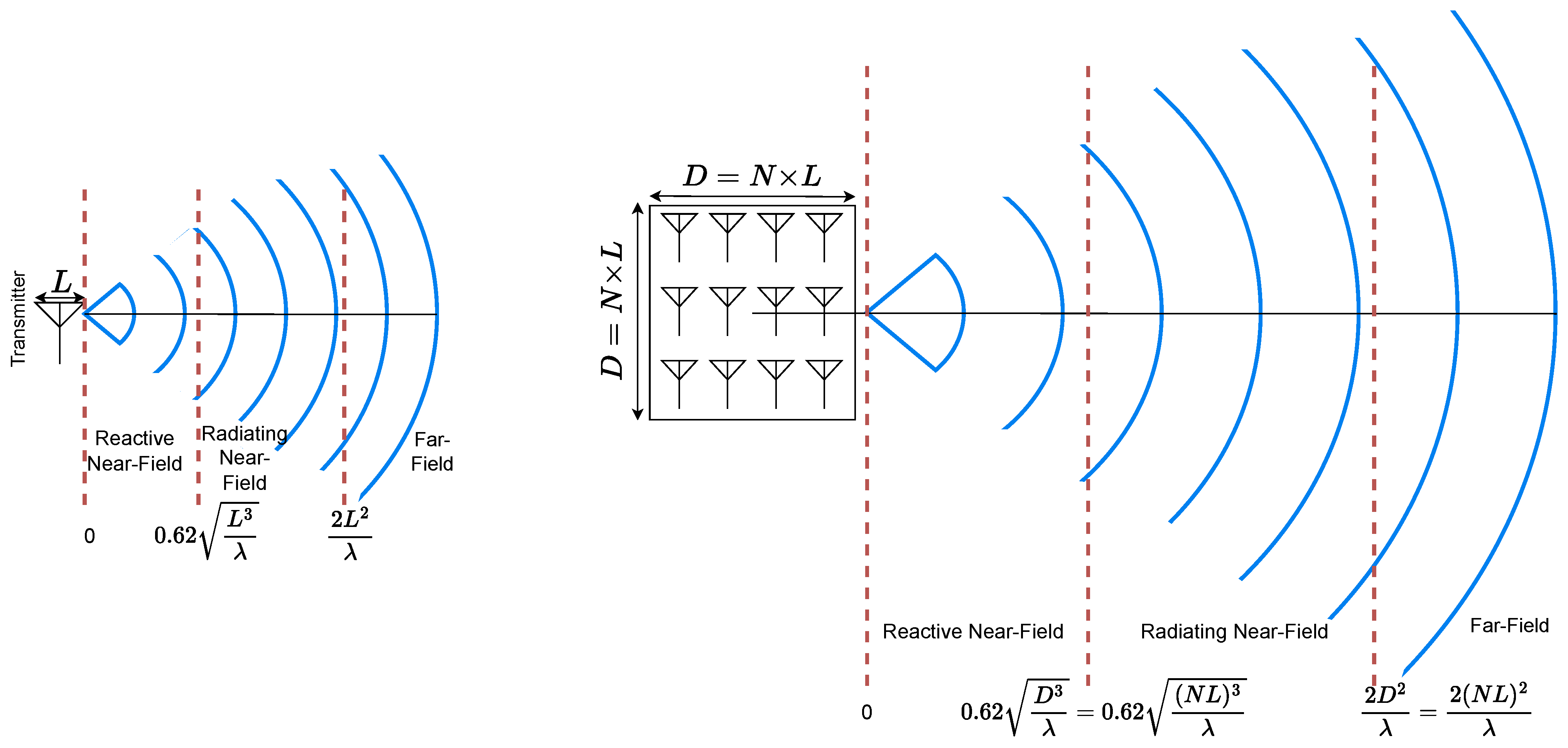
Before starting to investigate distributed beamforming, it is essential to understand the distinction between near-field and far-field radiation in the context of single antenna and large antenna aggregates, including distributed configurations such as our case study of WSNs, where sensors are assumed to communicate cooperatively using distributed beamforming techniques. This distinction depends on frequency, the aperture size of individual antennas, and, in the case of antenna arrays, the overall array dimensions, as illustrated in Figure 1. In the far-field, the distance between the antenna array and the receiver is sufficiently large that the differences in path lengths from each array element to the receiver can be considered negligible, and the wavefront can be approximated as planar. As outlined in [10], the minimum distance $d_F$ to reach the far-field region is typically defined by the Fraunhofer distance, which for an antenna aggregate of size $N\times N$ is given by

$$d_F\ge {\displaystyle \frac{2D^2}{\lambda }}$$

(1)

where $D=N\times L$, L is the physical size of a single antenna element, and $\lambda$ is the wavelength.

On the other hand, the near-field region can be sub-divided into two areas: the reactive near-field, dominated by evanescent waves and magnetic induction, which occurs at distances below

$$d_R\le 0.62\sqrt{{\displaystyle \frac{D^3}{\lambda }}}$$

(2)

and the radiating near-field (also known as the Fresnel region), which lies between $d_R$ and $d_F$, as illustrated in Figure 1.

For distances greater than or equal to the Fraunhofer distance $d_F$, the differences in path lengths from each array element (or node) to the receiver are negligible, making phase adjustments for beamforming in the far-field unnecessary. However, due to the typically large distances required to satisfy the Fraunhofer condition, especially at higher frequencies and for large antenna aggregates, this study focuses on the radiating near-field region.

In the context of WSNs, the receiver is generally in the far-field of each individual sensor but in the near-field of the entire sensor network. Therefore, our analysis concentrates on the radiating near-field, where the distance to the receiver is short enough to cause significant phase and/or amplitude variations across the array, yet sufficiently large to neglect direct hardware interactions between transmitter and receiver [12].

Figure 1. Near- and far-field regions [13]: (left) single antenna (right) antenna array.

Figure 1. Near- and far-field regions [13]: (left) single antenna (right) antenna array.

To establish effective distributed beamforming, precise synchronisation among the nodes of the system is essential. This synchronisation process involves carefully adjusting the timing of each node’s transmission, either by delaying or advancing its output signal, to ensure that the signal components from the desired direction arrive at the receiver in phase. This temporal alignment enables constructive interference among the signals, resulting in a significant enhancement of the received signal strength [14]. Figure 2 represents a possible sensor distribution.

Let $s_n\left(t\right)$ be the transmitted signal from the $n^{th}$ sensor being obtained by applying a phase shift ${\theta }_n$ to the measured data, $x\left(t\right)$ according to Equation (3):

$$s_n\left(t\right)=\Re \{x\left(t\right)e^{j{w}_{c}t}\}=\Re \{x\left(t\right)e^{j{w}_c(t_0-t_{d_n})}\}$$

(3)

Since we assume that all nodes are perfectly synchronized transmitting in $t_0=0$, we can simplify this equation, obtaining Equation (4):

$$s_n\left(t\right)=\Re \{x\left(t\right)e^{-j{w}_c{t}_{d_n}}\}=\Re \{x\left(t\right)e^{-j{\theta }_n}\}$$

(4)

This phase adjustment, ${\theta }_n$, is crucial for achieving in-phase addition at the receiver and maximizing the received signal strength.

The required phase shift for each node, ${\theta }_n$, can be calculated based on its distance from the receiver, as defined by Equation (5):

$${\theta }_n={\displaystyle \frac{\left(d_{max}-d_n\right)\times 2\pi }{\lambda }}$$

(5)

$d_n$ represents the distance between the $n_{th}$ sensor and the receiver, and $d_{max}$ is the maximum distance between any sensor and the receiver, serving as a reference. This phase adjustment ensures that the signals from all nodes arrive at the receiver with the appropriate phase shift, enabling coherent summation and maximising the received signal strength.

Due to the propagation distance, each transmitted signal experiences path loss, ${\beta }_n$, which can be modelled using the Friis free-space path loss Equation (6):

$${\beta }_n={\left({\displaystyle \frac{4\pi \times d_n}{\lambda }}\right)}^2$$

(6)

Considering the ideal phase shifts calculated previously, the received signal, $r\left(t\right)$, is obtained by summing the contributions from all sensors, taking into account the respective path losses:

$$\begin{array}{c}\hfill r\left(t\right)={\displaystyle \sum _{n=1}^N}{\displaystyle \frac{s_n\left(t\right)}{\sqrt{{\beta }_n}}}.\end{array}$$

(7)

This section has outlined the fundamental principles of distributed beamforming in WSNs. By synchronising transmissions and applying appropriate phase shifts to the signals from individual nodes, as defined by Equation (3), it is possible to achieve constructive interference at the receiver, enhancing the received signal strength and extending the communication range. However, the performance of distributed beamforming is significantly influenced by node position accuracy and path loss. In the following section, we investigate the impact of the number of nodes on the phase error variance, employing the Cramer–Rao Lower Bound (CRB).

3. Position-Based Distributed Beamforming: System Model and Methods

This study investigates distributed beamforming in WSNs, leveraging the knowledge of sensor positions to determine the appropriate phase adjustment for each node to perform beamforming. A simulation testbed is employed to evaluate the impact of inaccurate position information on beamforming performance. We assume the presence of an anchor node responsible for position estimation. This anchor node transmits its estimated positions, along with the receiver’s position, to all other nodes in the network. Upon receiving this information, each node calculates its required phase adjustment.

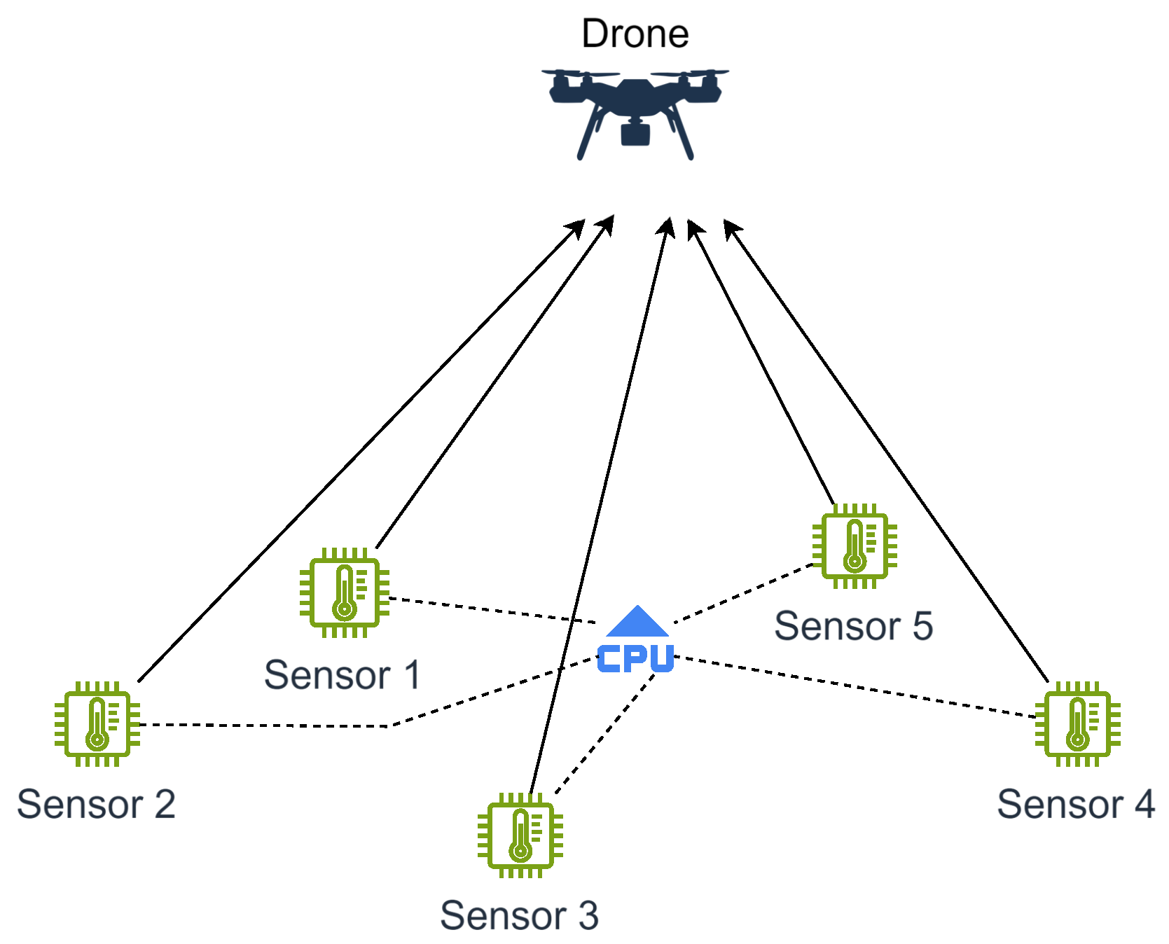
A two-dimensional schematic of the simulated environment is depicted in Figure 3. The system comprises multiple sensor nodes, represented as temperature sensors for illustrative purposes. These nodes are assumed to be coplanar, residing within a single plane. A Central Processing Unit (CPU) or an equivalent processing unit with a fixed and known position, is responsible for determining the absolute positions of the sensors within the simulation. However, the communication link between the sensors and the CPU is not explicitly modelled in this study. Instead, we focus on the cooperative communication between the sensors and a designated receiver—such as a drone, whose position is known—that captures the transmitted signals. Accurate time synchronization among sensors is essential for enabling effective cooperative beamforming. In this work, we assume that such synchronization has already been achieved using state-of-the-art techniques [15,16], as our primary objective is to investigate the impact of sensor position accuracy on the performance of distributed beamforming.

The system parameters used in the simulations are summarised in

Table 1. Simulation parameters.

Parameter	Value	Unit
Frequency (f)	433	MHz
Propagation Speed (c)	$3\times {10}^8$	m/s
Signal-to-Noise Ratio ($SNR$)	$[-20;20]$	dB
Number of Sensors (N)	40	-
Error Standard Deviation ($\sigma$)	$[0,0.025,\dots 0.1]\times \sqrt{\lambda }$	m
Field side	100	m

.

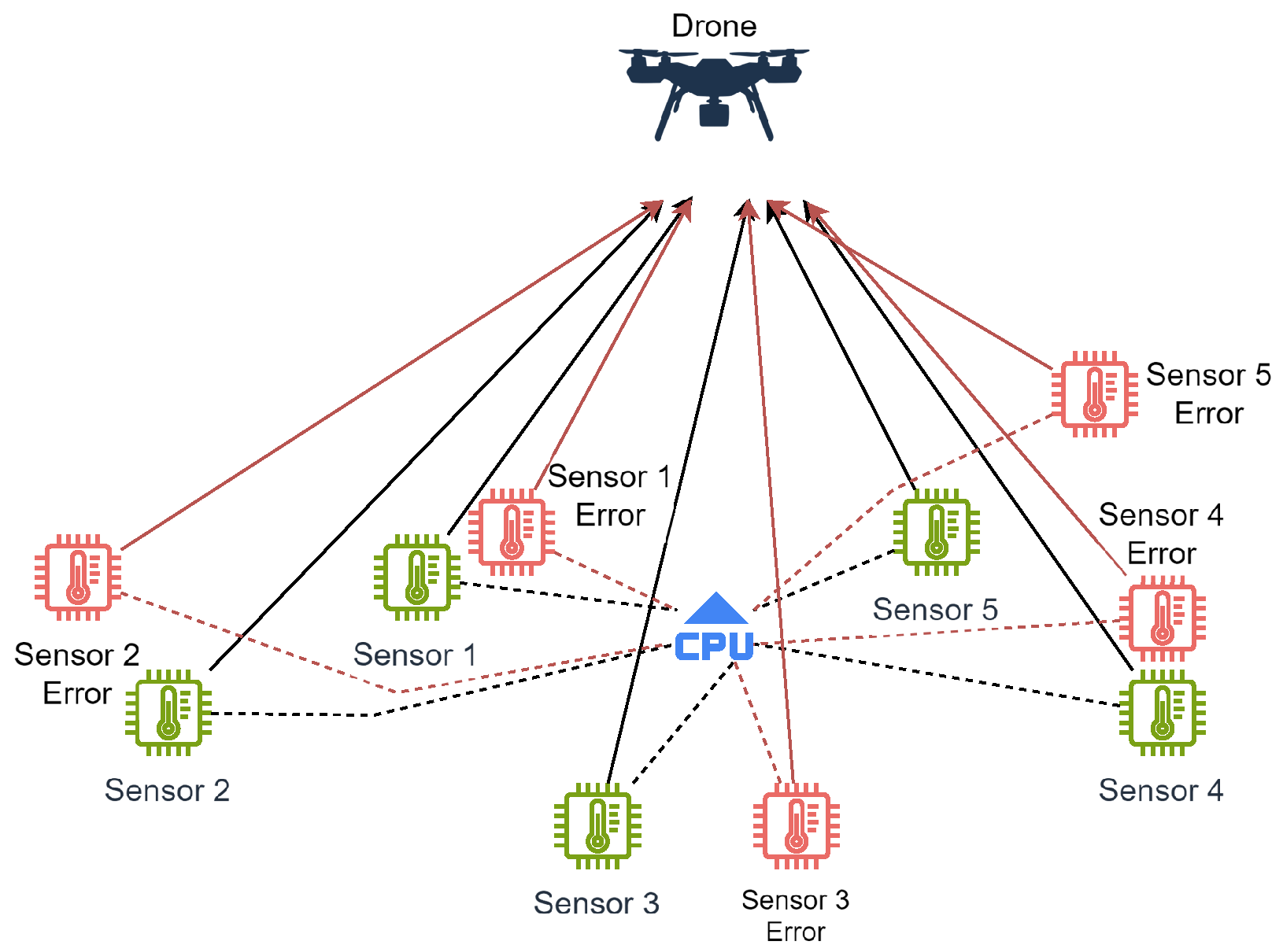
With the system characteristics defined, Gaussian Minimum Shift Keying (GMSK) signals are transmitted from each node. GMSK modulation is widely used in Internet of Things (IoT) systems because of its low power requirements, high accuracy, and noise robustness as it maintains a constant envelope, which also leads to reliable performances for low-powered sensors [17]. Then, random position errors are introduced to the sensor node locations to simulate realistic deployment scenarios, as illustrated in Figure 4. Additive White Gaussian Noise (AWGN) is added to the composite received signal to achieve a specified SNR.

Position errors are generated using a Gaussian random number generator with a predefined standard deviation. These error values are then added to the absolute positions of the sensor nodes, simulating inaccuracies in position estimation. These position errors lead to incorrect phase adjustments in the beamforming process, increasing the number of errors in the receiver, ultimately resulting in a degraded Bit Error Rate (BER), as is possible to conclude analysing Equation (8) and as will be shown later in Section 5.

$$BER={\displaystyle \frac{N_{errors}}{N_{bits}}}$$

(8)

4. The Number of Sensors and Cramér–Rao Bound

The number of sensor nodes significantly influences the system’s performance, affecting energy efficiency and the resulting beam pattern. Increasing the number of nodes generally leads to a narrower main beam and a reduction in the number of side lobes, improving the directivity of the beam [6,18,19]. Figure 5 illustrates this effect by comparing the beampatterns of two linear arrays with four and eight elements.

Furthermore, the number of sensors can significantly impact the system’s accuracy. To evaluate the theoretical limits of position estimation accuracy, we employ the Cramer–Rao Bound (CRB) [20]. The CRB provides a lower bound on the variance of any unbiased estimator, offering a valuable benchmark for assessing the achievable accuracy in the presence of noise and uncertainties. While other bounds exist, the CRB is widely recognized for its effectiveness and unbiased nature in estimating the precision of parameter estimation, as it is directly derived from the Fisher Information Matrix (FIM) [20].

In our case, we are concerned with the system’s performance when there is an error in the position of the sensors, which leads to an error in the computed phase shift (5) significantly affecting the Bit Error Rate (BER) performance, especially when fewer sensors are contributing.

We can use the FIM to find the lower bound on the phase shift resulting from errors in the sensors’ positions. The FIM can be obtained from the gradient, $\nabla \varphi$, of the phase shift Formula (5) with respect to the coordinates of the sensors’ positions, as given by

$$\nabla \varphi ={\displaystyle \frac{2\pi }{\lambda }}\left({\overline{S}}_{(x,y,z)}-D_{(x,y,z)}\right)\oslash \left|\right|{\overline{S}}_{(x,y,z)}-D_{(x,y,z)}\left|\right|$$

(9)

where ${\overline{S}}_{(x,y,z)}$ is the matrix of sensor position coordinates, with one sensor per row; the row vector $D_{(x,y,z)}$ represents the true coordinates of the drone receiver; $\left|\right|{\overline{S}}_{(x,y,z)}-D_{(x,y,z)}\left|\right|$ is the vector of distances of each sensor to the drone; and ⊘ denotes element-wise Hadamard division. The FIM matrix is thus given by

$$FIM=\nabla \varphi \odot \nabla {\varphi }^{\prime }$$

(10)

where ${(}^{\prime })$ denotes the transpose operation and $(\odot )$ represents the Hadamard dot product between the gradients.

5. Results

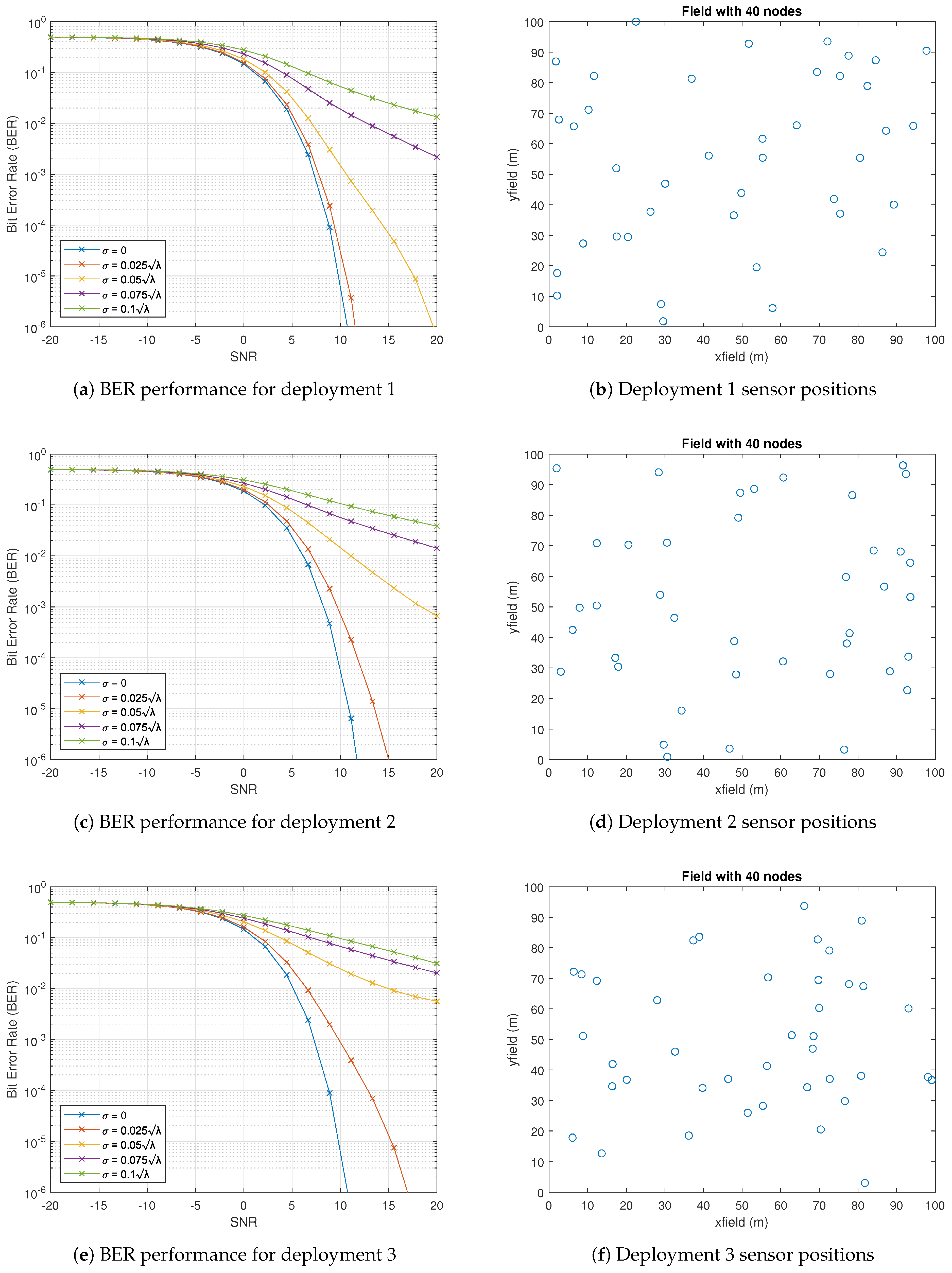
Using the equations presented previously and applying the chosen parameters, several simulations were made, obtaining the results presented in this section. First, we present the beamforming performance under sensor position errors, followed by the CRB results, based on the system specifications shown in Table 1. To analyse the impact of these errors, three distinct deployments, each with significantly different sensor distributions, were considered. By introducing errors, we expect the resulting BER graphs to reveal variations in system performance. This can be confirmed by analyzing the results presented in Figure 6.

Figure 6 presents BER performance assuming a random Gaussian error in each sensor’s position, with the variance expressed as a function of the carrier wavelength. The case where the variance is zero represents the ideal scenario with no error in sensor position estimation. The performance gap between the ideally scenario (where sensor positions are accurately known) and the non-ideal cases widens as the SNR increases. This indicates that, in high-SNR conditions, performance can be severely degraded due to destructive beamforming caused by position errors. These differences highlight the importance of analyzing the sensor distribution before deploying a non-uniformly spaced WSN, as our objective is to minimize the transmitted power while maintaining a minimum SNR that satisfies the BER threshold through beamforming, ensuring reliable data reception.

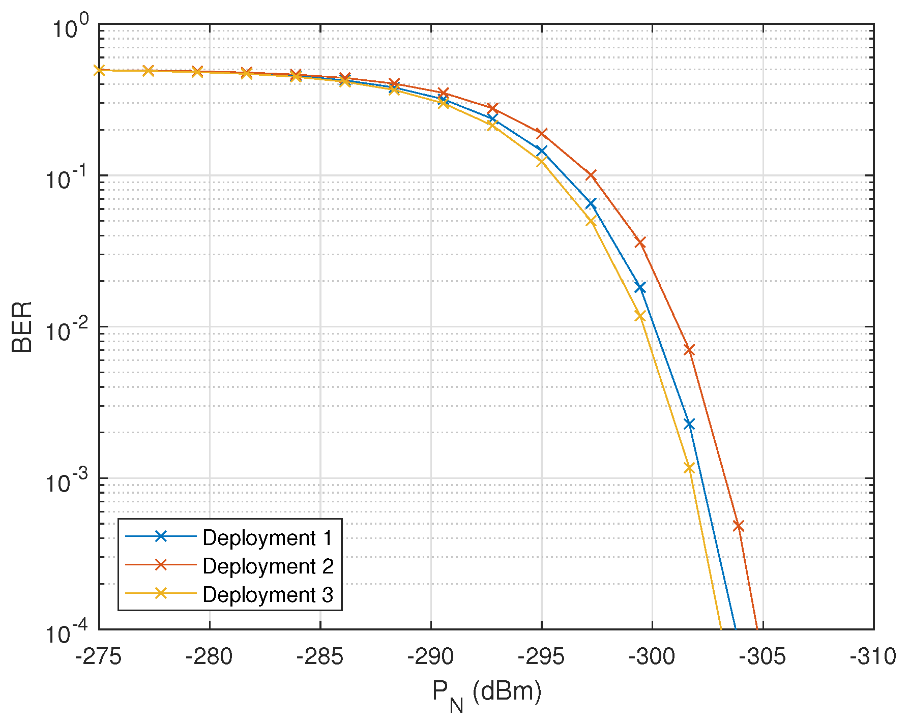
As previously discussed, network topology is crucial in system performance, particularly concerning received signal power. To illustrate this, in Figure 7, we present the BER performance for three different deployments. We assume that all sensors transmit at maximum power and that the drone is positioned at the center of the field. The results are plotted as a function of the noise power upon the receiver drone.

As anticipated, the received signal power decreased significantly with variations in network topology for a fixed number of sensors. This is a result of the increased distance between transmitters and the receiver, which leads to higher path loss throughout the system. Therefore, receiver position and position estimation accuracy are critical considerations for successfully implementing such systems, reinforcing the need to simulate the system before applying it in a real-world scenario.

Finally, for the CRB, we calculate the FIM and the CRB as the inverse of the FIM [20]. The results show the normalised trace values of the CRB in the x,y, and z directions.

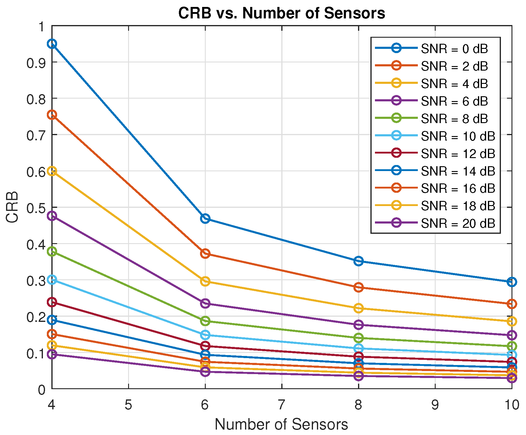
The graph shows that if we have a high SNR, the accuracy would almost remain constant even if more sensors were added. Thus, we can reduce the number of sensors if we correctly choose the sensors associated with the drone, which all contribute constructively.

6. Discussion

Based on the results obtained, it is essential to analyse the performance of each deployment, as shown in Figure 6. Despite the differences in sensor distribution (deployments 2 and 3), Figure 6d,f exhibit similar behaviour in terms of sensor position errors. In contrast, for deployment 1, Figure 6b shows lower signal degradation, which can be attributed to a sensor distribution that enables a more favourable drone positioning for the scenario defined in this model. This leads us to a need to optimise the position of the receiver according to the sensor distribution in order to achieve a higher SNR and, consequently, improved BER performance.

Following the previous analysis, deployment 1 appears to have a higher signal power at the drone. This can be confirmed when we apply the same noise power, $P_N$, to every distribution in the ideal case. As shown in Figure 7, deployment 3 exhibits better BER performance at lower $P_N$, indicating that it has a higher SNR. This can be regarded as a case where the position selected by the drone to collect data from the sensors is more favourable, given the sensor deployment configuration. This leaves room for future work focused on determining the optimal drone positioning within WSNs, considering positioning errors in the sensors, with the goal of maximising communication BER performance and minimising the impairments caused by positioning inaccuracies.

Finally, we analyse the number of sensors required to achieve satisfactory accuracy. From Figure 8, it can be seen that for different levels of SNR, we can improve the system’s accuracy by increasing the number of sensors. However, after a certain point of increasing the sensors, the accuracy is not affected significantly, and an optimum number of sensors for the desired SNR can be decided from this. For instance, if we operate at 10 dB satisfying the required BER, then the feasible number of sensors required is eight. Increasing the number of sensors in the system would not change the system further, and we would just be wasting the power of the remaining utilised sensors.

7. Conclusions

This work investigated the performance of distributed beamforming in WSNs with a focus on the impact of position errors by developing a comprehensive simulation testbed. Real-world WSN deployments present numerous challenges, making software simulations essential for gaining insights into system behaviour and optimising implementation strategies. Our simulations provided a valuable tool for modelling individual components and complex processes, particularly those involving multidimensional arrays, allowing us to isolate and analyse the impact of key parameters.

Our results underscore the critical importance of accurate beamforming for maximising received signal power. While conventional beamforming in uniformly spaced arrays inherently mitigates localisation challenges, distributed beamforming exhibits a greater sensitivity to sensor placement. We demonstrated that accurate sensor location information is fundamental for successful distributed beamforming, as imprecise implementations can lead to destructive interference and significant signal degradation.

In conclusion, our simulation platform effectively demonstrates the functionality of distributed beamforming in WSNs and confirms that the number of sensors, position accuracy, and receiver localisation are critical factors for maintaining a desired signal quality. These findings highlight the need for localisation algorithms that minimise position error variance to achieve robust signal quality. Ultimately, this work contributes to optimising WSN performance and enabling reliable deployment in challenging environments.