A Multi-Head LSTM Architecture for Bankruptcy Prediction with Time Series Accounting Data

Abstract

With the recent advances in machine learning (ML), several models have been successfully applied to financial and accounting data to predict the likelihood of companies’ bankruptcy. However, time series have received little attention in the literature, with a lack of studies on the application of deep learning sequence models such as Recurrent Neural Networks (RNNs) and the recent Attention-based models in general. In this research work, we investigated the application of Long Short-Term Memory (LSTM) networks to exploit time series of accounting data for bankruptcy prediction. The main contributions of our work are the following: (a) We proposed a multi-head LSTM that models each financial variable in a time window independently and compared it with a single-input LSTM and other traditional ML models. The multi-head LSTM outperformed all the other models. (b) We identified the optimal time series length for bankruptcy prediction to be equal to 4 years of accounting data. (c) We made public the dataset we used for the experiments which includes data from 8262 different public companies in the American stock market generated in the period between 1999 and 2018. Furthermore, we proved the efficacy of the multi-head LSTM model in terms of fewer false positives and the better division of the two classes.

1. Introduction

Predicting corporate bankruptcy is one of the most fundamental tasks in credit risk assessment. Especially after the 2007/2008 financial crisis, it has become a top priority for most financial institutions, fund managers, and lenders, due to the substantial financial damage that can result from corporate default. Indeed, corporate failure may result in high social costs and further propagate recession, especially when it involves a large number of companies simultaneously and affects the entire economy [1]. Since the 2008 financial crisis, researchers and practitioners have made several efforts to build models that can efficiently assess the likelihood of company default, especially for public companies in the stock market. Regulators also benefit from accurate bankruptcy forecasting models since they can monitor the financial health of institutions and curb systemic risks [2].

Since Altman presented his bankruptcy forecasting model in 1968 [3], research has shown that accounting-based ratios and stock market data can signal whether a firm is likely to face severe difficulties, such as bankruptcy. Although default prediction models have been studied for decades, we still lack a definite theory of predicting corporate failure [4]. The lack of a theoretical framework led to the adoption of a common development methodology where research is more focused on identifying discriminant features using a trial-and-error approach [5,6].

The advent of machine learning (ML) and its advances offered novel possibilities for bankruptcy prediction in terms of learning models with several attempts using different ML algorithms and techniques such as the Support Vector Machine (SVM) [7], boosting techniques [8], discriminant analysis [9], and neural networks. Moreover, different architectures have been evaluated to identify effective decision boundaries for this binary classification problem, such as the least absolute shrinkage and selection operator [10], the dynamic slacks-based model [11], and two-stage classification [12].

However, a common element of these models is the punctual application of market-based and accounting-based variables, while time series have received little attention, and there is insufficient literature concerning the application of the most recent deep learning models for sequence data such as Recurrent Neural Networks and Attention-based models. In this paper, we compare two different Recurrent Neural Network (RNN) architectures based on Long Short-Term Memory (LSTM) units to predict bankruptcy from a time series of accounting data. In general, RNN-based models have been seldom investigated in the recent literature. In particular, we used a single-input RNN and a multi-head RNN that modeled each financial variable within a time window, independently exploiting the latent representation learned only in the last stage of the bankruptcy classification process. The idea of building a multi-head architecture aimed to investigate whether an attention method pipeline can outperform a classical RNN setting when learning a latent representation of the company by focusing on each time series independently.

The main contributions of this paper are the following:

• We proposed a multi-head LSTM for bankruptcy prediction on time series data.
• We investigated the optimal time window of financial variables to predict bankruptcy with a comparison among the main state-of-the-art approaches in machine learning and deep learning. Experiments were performed on public companies traded in the American stock market with data available between 2000 and 2018.
• We anonymized our dataset and made it public for the scientific community for further investigations and to provide a benchmark for future studies on this topic.
• We analyzed our models on the test set, using T-SNE [13] to show the ability of our models to capture patterns. We also performed an in-depth analysis of false positives.

2. Related Works

In traditional methods to forecast bankruptcies, Altman’s Z-score is the most prominent approach, but the Kralicek quick test and Taffler’s model also use scoring methodologies to provide ordinal rankings of default risk [14,15]. Altman, as well as Beaver and William, used discriminant analysis, which has been widely employed following their works, while Ohlson was the first to introduce a binary response model using explanatory variables and applying a logistic function [16,17]. Scoring methodologies have also been used to produce a binary response given a pre-set threshold. For example, Altman suggested the use of two thresholds, 1.81 and 2.99. According to this, an Altman’s Z-score above the 2.99 threshold means that firms are not predicted to default in the next two years, a score below 1.81 indicates that they are predicted to default, while a score between the two thresholds lies in a “zone of ignorance” where no clear decision can be taken. However, even though many practitioners use these thresholds, in Altman’s view, this is an unfortunate practice since over the past 50 years, credit-worthiness dynamics and trends have changed so dramatically that the original zone cutoffs are no longer relevant [18].

Even though many authors continue to work on traditional bankruptcy models, the exploration of machine learning applications for corporate default has been more prevalent in recent years [5,6,12,19,20,21,22]. Barboza et al. showed that, on average, machine learning models exhibit 10% higher accuracy compared to traditional ones. Specifically, in this study, Support Vector Machines (SVMs), Random Forests (RFs), and bagging and boosting techniques were tested for predicting bankruptcy events and compared with results from discriminant analysis, logistic regression, and neural networks. The authors found that bagging, boosting, and RFs outperformed all other models [23]. However, Altman, in his recent book, discussed a trade-off between models’ performance and explainability when using machine learning models, expressing skepticism as to whether practitioners would adopt “black-box” methods but acknowledging the superiority of the models in assessing corporate distress [18].

Considering that the results regarding the superiority of these models are still inconclusive, new studies exploring different models, contexts, and datasets are relevant. Machine learning techniques like ensembles of classifiers were first explored for default prediction by Nanni et al. [24]. Kim et al. showed that the ensembles greatly outperformed standalone classifiers [25]. Wang et al. further analyzed the performance of ensemble models, finding that bagging outperformed boosting in average accuracy for all credit databases they used, as well as type I and type II errors [26]. In [27], some evidence was presented regarding the need to consider time series for survival probability estimation over the years and bankruptcy prediction, with some benchmarks that also prove that neural networks, when properly designed, can achieve better results with time-dependent accounting variables.

Barboza et al. also argued that a firm’s failure will likely be caused by difficulties over time, not just the year before bankruptcy. To incorporate the dynamic behavior of firms, they added new variables reflecting changes in financial metrics such as growth measures and changes [23]. Findings dating back to 1966 show that firms exhibit failure tendencies as much as five years before the actual event [16]. On the other hand, in 1998, Mossman et al. pointed out that models are only capable of predicting bankruptcy two years before the event, which improves to three years if used for multi-period corporate default prediction [28,29]. In most studies, ratios are analyzed backward in time starting with the bankruptcy event and going back until the model becomes unreliable or inaccurate. The time threshold for developing good classification models is two or three years, at most five, while Altman mentioned in his book that there are certain characteristics of bonds at birth that can significantly influence their default likelihood over up to ten years after issuance [16,18,28,29].

However, most of the bankruptcy prediction models in the literature do not take advantage of the sequential nature of the financial data. This lack of multi-period models was also emphasized in Kim et al.’s literature review [30]. One of the few studies that have leveraged the sequential nature of accounting data is that of Vochozka et al., who examined the performance of a Long Short-Term Memory (LSTM) model for bankruptcy prediction in the Czech manufacturing sector [31]. Kim et al. also used quarterly accounting data for non-financial industry companies and daily market data from January 2007 through December 2019 in both RNN and LSTM models, finding that RNNs made reasonable predictions in most situations, while both LSTMs and RNNs outperformed the logistic regression, Support Vector Machine, and Random Forest methodologies [32]. However, to the best of our knowledge, there are no studies of corporate bankruptcy that have examined a similar number of observations or leveraged time series data considering different time windows to predict defaults. Since it is difficult to make a fair comparison with the available literature (most of the datasets are either small or not usable with deep learning; or, more commonly, they have not been publicly released), we compared our deep learning model with all the algorithms presented in this section on our dataset. The dataset was publicly released for further investigations and comparisons, and it is available on GitHub (https://github.com/sowide/bankruptcy_dataset, accessed on 1 February 2024). See Section 4 for more details.

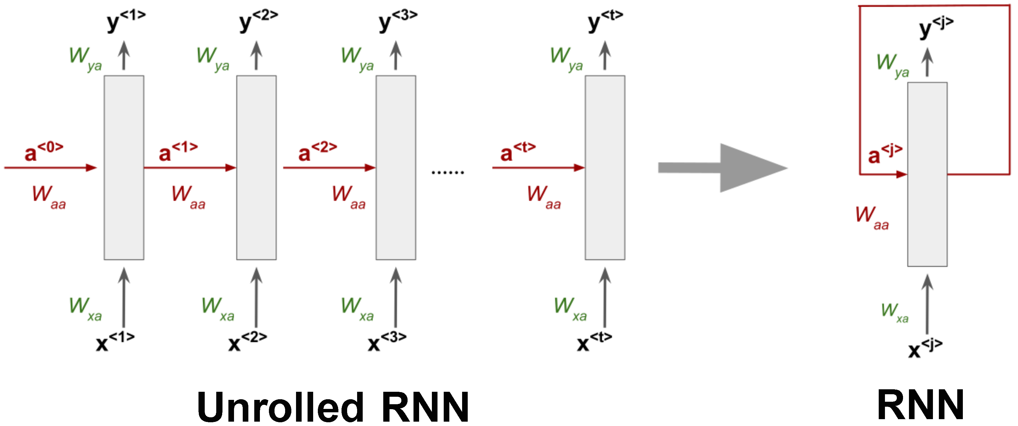
3. Recurrent Neural Networks

A Recurrent Neural Network (RNN) is a deep learning architecture that aims to process sequences of values in the form $x^{\left(1\right)}$, $x^{\left(2\right)}$.…., $x^{\left(t\right)}$. This ability is due to the network’s parameter sharing across different parts of a model, which makes it possible to extend and apply the model to examples of different forms. Moreover, parameter sharing also allows the model to preserve generalization across the sequence since the same parameters (weights) are used for each value of the time index, while a traditional fully connected feed-forward network would have separate parameters for each input feature. The time index refers to the position in the sequence. A Recurrent Neural Network is generally composed of a single unit of processing that produces an output y at each time step and has recurrent connections in general from the hidden units $a^{<j>}$ and optionally from the output. When an RNN has only recurrent connections from the hidden units, it processes an entire sequence and then produces a single output. Figure 1 shows a generic RNN structure that processes a sequence of t elements with recurrent connections only from the hidden units. Input, output, and recurrent hidden states are propagated using different weight matrices whose elements are learned during training via the back-propagation through time algorithm [33]. Equations (1) and (2) describe the internal behavior of an RNN unit. The initial hidden state $a^0$ is generally equal to zero. In general, for a generic time index j, the hidden state is computed as a weighted sum of the previous state $a^{j-1}$ and the current input $x^j$ plus a bias term. After that, an activation function $\sigma$ is applied to the result as in fully connected networks. The output at each time step only depends on the current internal state plus a different bias $b_y$. The two activation functions to estimate the hidden state and the output may differ. Additionally, the weight matrices $W_{aa}$, $W_{xa}$, and $W_{ya}$ play crucial roles in the computations:

• $W_{aa}$: Weight matrix from the previous hidden state $a^{<j-1>}$ to the current hidden state $a^{<j>}$.
• $W_{xa}$: Weight from the input at time j ($x^{<j>}$) to the current hidden state $a^{<j>}$.
• $W_{ya}$: Weight matrix from the hidden state $a^{<j>}$ to the output $y^{<j>}$.

$$a^{<j>}=\sigma (W_{aa}·a^{<j-1>}+W_{xa}·x^{<j>}+b_a)$$

(1)

$$y^{<j>}=\sigma (W_{ya}·a^{<j>}+b_y)$$

(2)

In this way, Recurrent Neural Networks can process entire sequences and can use contextual information when mapping inputs into outputs. Unfortunately, for standard RNN architectures, the range of context that can be in practice is quite limited, especially for long sequences and for more than one sequence in the input (matrix input). The major issue is that the influence of a given input on the hidden state, and therefore on the network output, either decays or blows up exponentially as it cycles around the network’s recurrent connections. This effect is often referred to in the literature as the vanishing gradient problem [34]. 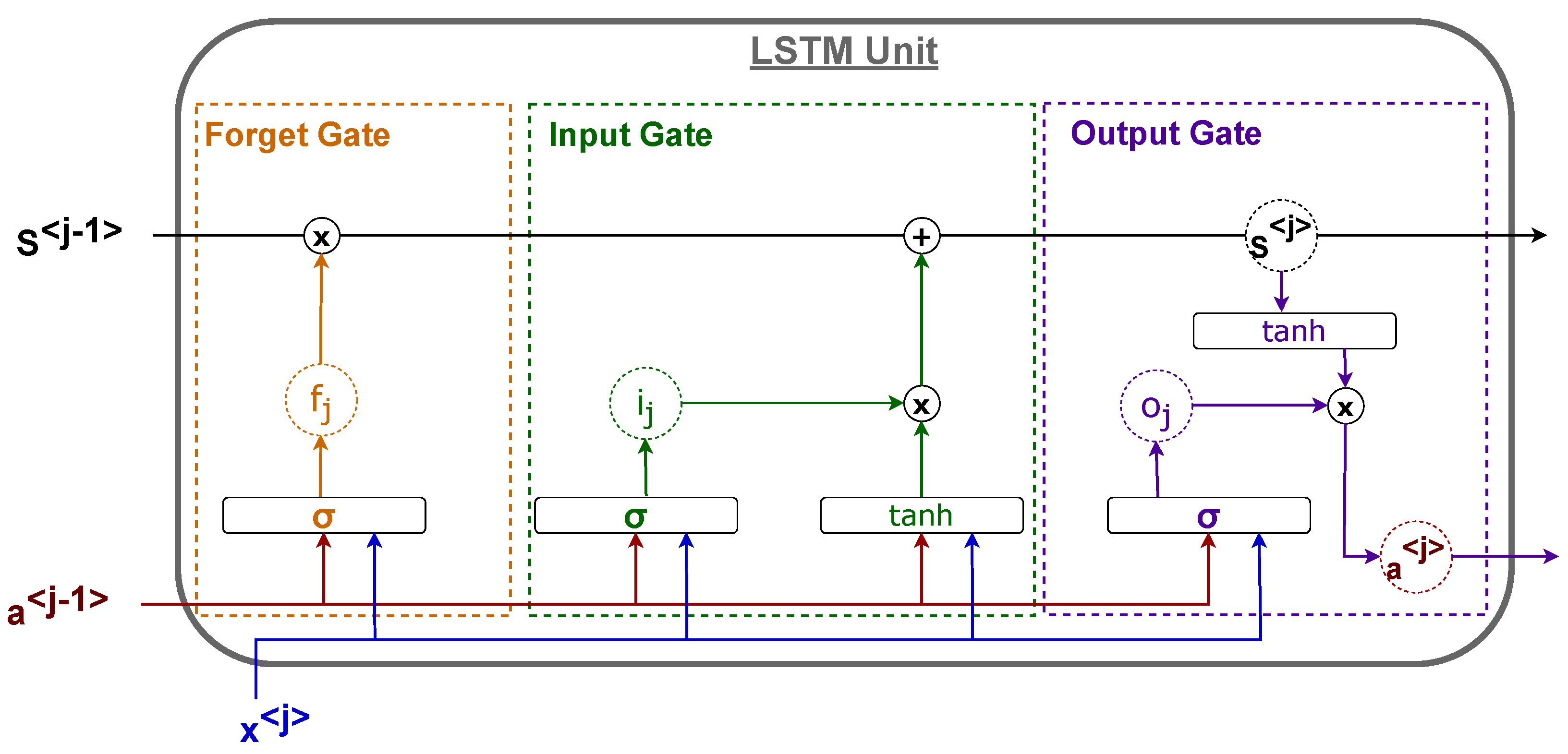Several approaches have been presented to solve this issue like the Long-Short Term Memory (LSTM) architecture [35] and the Gated Recurrent Unit (GRU) [36]. In both architectures, several additional components (called gates) are introduced inside the unit to extend the memory of the network in case of a long sequence so that the first part of each sequence is not forgotten when producing the output (long-term dependency problem) and to prevent the gradient from vanishing. We describe LSTM since it is the architecture used in this research work and because the GRU unit can be taken back to a particular case of the LSTM unit. The basic idea is to employ a unit state $s_j$ to retain the information taken from earlier time indexes in the sequence. The unit is composed of three gates:

• Forget Gate: This determines the amount of information that should be retrieved from the previous unit state.
• Input Gate: This defines the amount of information from the new input $x^{<j>}$ that should be used to update the unit’s internal state.
• Output Gate: This defines the output of the unit as a function of its current unit state.

An example of an LSTM unit is presented in Figure 2. Every connection is weighted by a different matrix whose elements are estimated using back-propagation through time as in basic RNNs.

4. Dataset

In this section, we present the dataset used in the experiments, which we have made available to the scientific community. The procedure used to build the dataset can be described as follows:

• We collected data on 8262 different public companies in the American stock market between 1999 and 2018. We selected the same companies used in [37,38] since these companies were considered a good approximation of the American stock market (NYSE and NASDAQ) in those time intervals.
• For these firms, we collected 18 financial variables, often used for bankruptcy prediction, for each year. In bankruptcy prediction, it is common to consider accounting information and up-to-date market information that may reflect the company’s liability and profitability. We selected the variables listed in

  Table 1. The 18 numerical bankruptcy features.

  Variable Name	Variable Name
  Current assets	Total assets
  Cost of goods sold	Total long-term debt
  Depreciation and amortization	EBIT
  EBITDA	Gross profit
  Inventory	Total current liabilities
  Net income	Retained earnings
  Total receivables	Total revenue
  Market value	Total liabilities
  Net sales	Total operating expenses

  as the minimum common set found in the literature [3,10,39] and to have a dataset for twenty years without missing observations.
• For all the experiments presented in Section 5, we only considered firms with at least 5 years of activity since we aimed to first identify the time window that optimized the bankruptcy prediction accuracy.

Each company was labeled every year depending on its status the following year. According to the Security Exchange Commission (SEC), a company in the American market is considered bankrupted in two cases:

• If the firm’s management files Chapter 11 of the Bankruptcy Code to “reorganize” its business—management continues to run the day-to-day business operations, but all significant business decisions must be approved by a bankruptcy court.
• If the firm’s management files Chapter 7 of the Bankruptcy Code—the company stops all operations and goes completely out of business.

In both cases, we labeled the fiscal year before the chapter filing as “bankruptcy” (1). Otherwise, the company was considered healthy (0). In light of this, our dataset enables a model to learn how to predict bankruptcy at least one year before it happens.

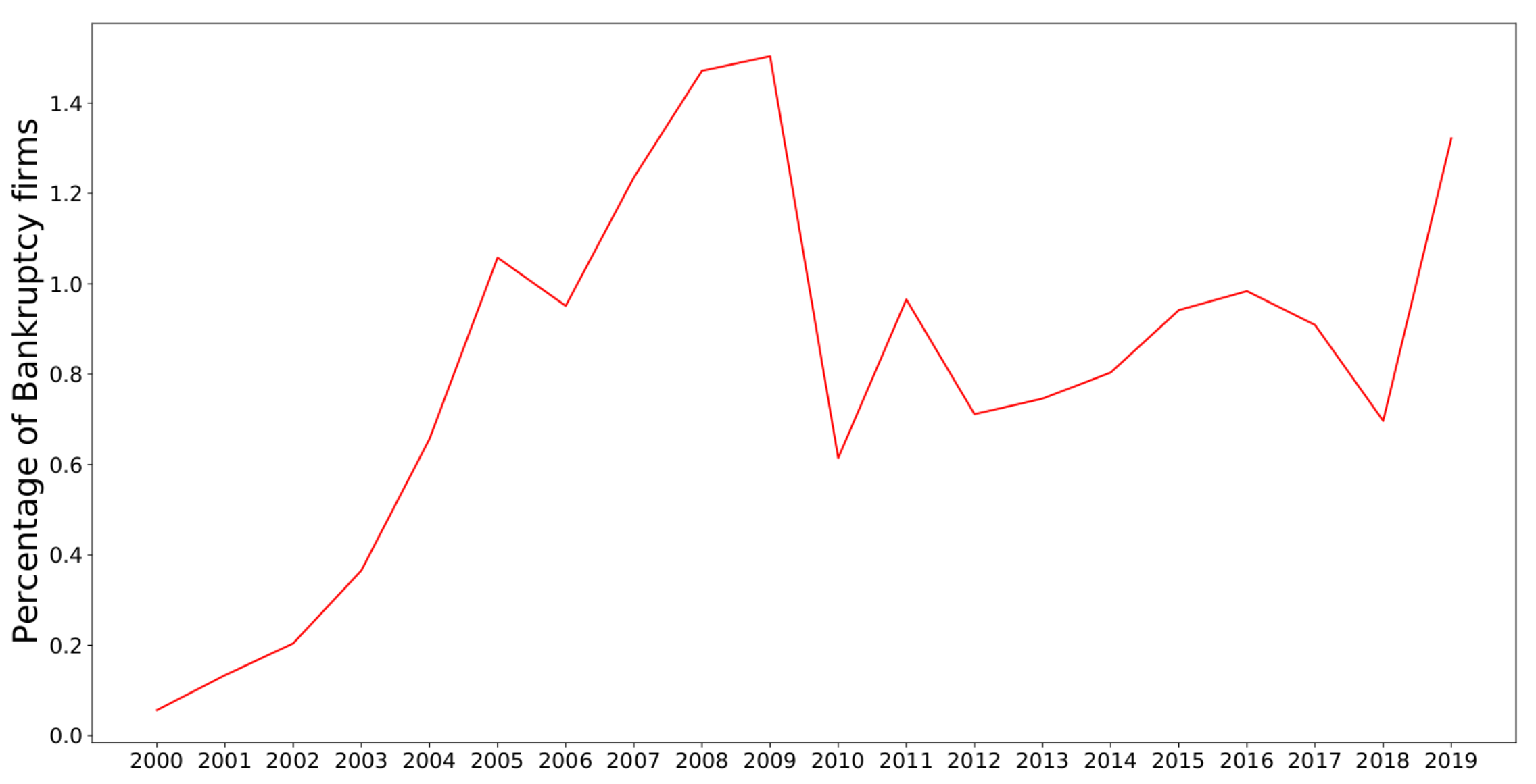
There is typically a strong imbalance in bankruptcy datasets since the number of firms that declare default each year is usually a small percentage below 1% of the available firms in the market. However, in some periods, bankruptcy rates are higher than usual— for example, during the Dot-Com Bubble in the early 2000s and the Great Recession between 2007 and 2008. Our dataset reflects this condition, as shown in Figure 3. The dataset firm distribution by year is presented in

Table 2. Firm distribution by year in the dataset.

Year	Total Firms	Bankrupt Firms	Year	Total Firms	Bankrupt Firms
2000	5308	3	2010	3743	23
2001	5226	7	2011	3625	35
2002	4897	10	2012	3513	25
2003	4651	17	2013	3485	26
2004	4417	29	2014	3484	28
2005	4348	46	2015	3504	33
2006	4205	40	2016	3354	33
2007	4128	51	2017	3191	29
2008	4009	59	2018	3014	21
2009	3857	58	2019	2723	36

.

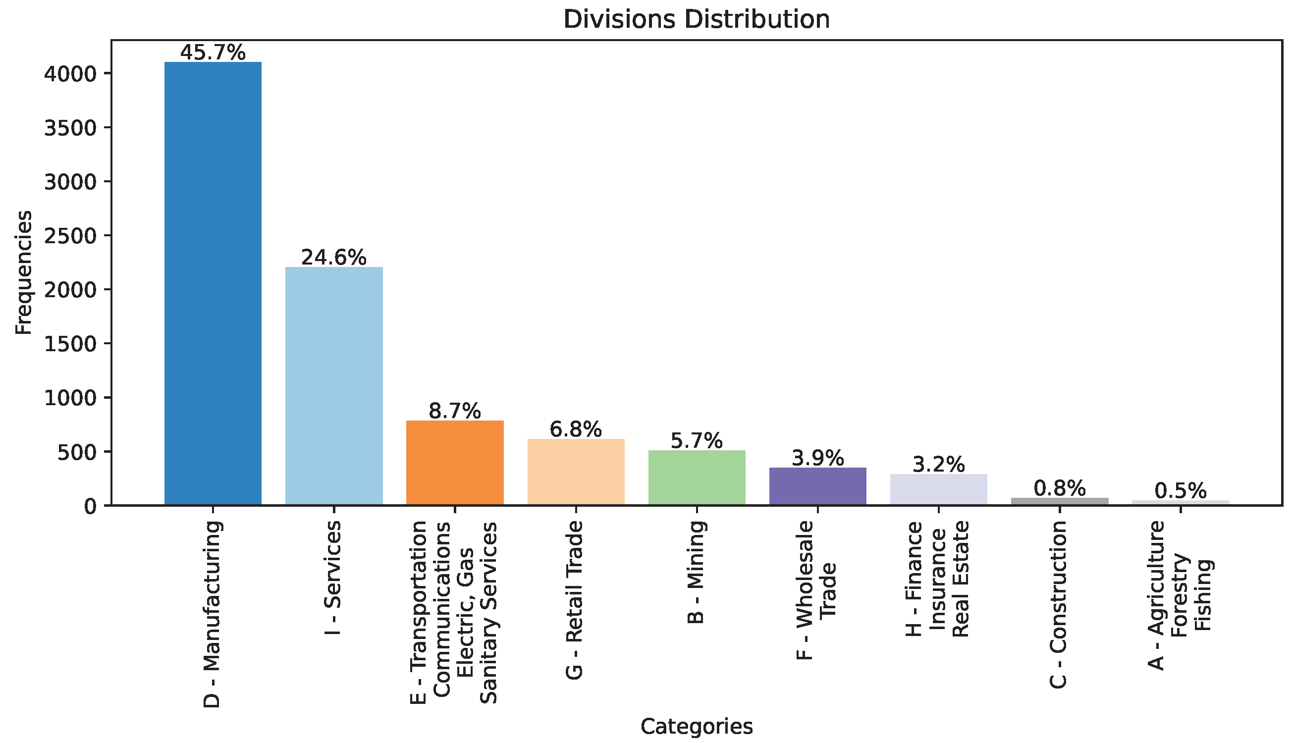
Moreover, each company in the dataset was categorized using the Standard Industrial Classification (SIC) system, developed by the US government to classify businesses based on their primary economic activities. The SIC codes not only distinguish firms but also enable more granular categorization by specifying major groups within each firm [40]. Major groups represent specific subcategories that define the business-type activities undertaken by these companies. The inclusion of SIC codes and major groups allowed us to conduct a deep analysis of bankruptcy trends across a wide range of industries. This classification system helps researchers and analysts gain insights into the economic factors and market dynamics affecting various sectors of the American economy, making it a valuable resource for studying bankruptcy patterns and their implications for different industries and major groups. Additionally, we generated the frequency distribution chart in Figure 4 to represent the companies’ distribution across different divisions within our dataset. This histogram provides a clear overview of the prevalence of companies in each division, highlighting which sectors of the economy were more heavily represented among the bankrupt firms. It helped us evaluate the overall dataset composition and identify any potential trends or disparities in bankruptcy occurrences across divisions. In this work, we performed a comprehensive examination of the dataset, with a particular focus on the division distribution.

Finally, the resulting dataset of 78,682 firm-year observations was divided into three subsets according to the time period: a training set, a validation set, and a test set. We used data from 1999 to 2011 for training, data from 2012 to 2014 for validation and model comparison, and the remaining years from 2015 to 2018 as a test set to assess the ability of the models to generalize their prediction to unseen data.

5. Hardware Specifications

All the experiments described in this work were performed using a Linux Ubuntu server with the following hardware specifications:

• CPU: Intel i9-10900 @2.80 GHZ
• GPU: Nvidia RTX 3090 (24 GB).
• RAM: 32 GB DDR4—2667 MHz.
• Motherboard: Z490-A PRO (MS-7C75).

6. Metrics

We implemented the bankruptcy prediction as a binary prediction task where the positive class (1) indicated bankruptcy in the next year and the negative class (0) meant that a company was classified as healthy in the next year. In order to compare our models and prove their effectiveness, we used different metrics that took into account the imbalanced condition of the validation and test sets. Consider the following quantities for the default prediction:

• True Positive (TP): The number of actually defaulted companies that were correctly predicted as bankrupted.
• False Negative (FN): The number of actually defaulted companies that were wrongly predicted as healthy firms.
• True Negative (TN): The number of actually healthy companies that were correctly predicted as healthy.
• False Positive (FP): The number of actually healthy companies that were wrongly predicted as bankrupted by the model.

Since the validation and test sets were both imbalanced with a prevalence of healthy companies, we did not compare the models in terms of model accuracy. Indeed, the proportion of correct matches would be ineffective in assessing the model performance. Instead, we computed each class’s precision, recall, and $F_1$ scores. This is highlighted because, in predicting bankruptcy, an error has a different cost depending on the class that has been incorrectly predicted. The consequences of erroneously classifying a financially distressed company as healthy incur a significantly higher cost than misclassifying a healthy company as financially distressed. In light of this, the precision achieved for a class is the accuracy of that class’ predictions. The recall (sensitivity) is the ratio of the class instances that were correctly detected as such by the classifier. The $F_1$ score is the harmonic mean of precision and recall: whereas the regular mean treats all values equally, the harmonic mean gives more weight to low values. Consequently, we obtained a high $F_1$ score for a certain class only if its precision and recall were high. Equations (3)–(5) report how these quantities are computed for the positive class. The definitions for the negative class are the same but with positives exchanged for negatives.

$$Precision=\frac{TP}{(TP+FP)}$$

(3)

$$Recall=\frac{TP}{(TP+FN)}$$

(4)

$$F_{1}score=\frac{2}{\frac{1}{Precision}+\frac{1}{Recall}}$$

(5)

Moreover, we report three global metrics for the classifier that were selected because they enabled an overall evaluation of the classifier for both classes without being influenced by the dataset imbalance:

• The Area Under the Curve (AUC) measures the ability of a classifier to distinguish between classes and is used as a summary of the Receiver Operating Characteristic (ROC) curve. The ROC curve is created by plotting the true-positive rate (TPR) against the false-positive rate (FPR) at various threshold settings.
• The macro $F_1$ score is computed as the arithmetic mean of the $F_1$ score of all the classes.
• The micro $F_1$ score is used to assess the quality of multi-label binary problems. It measures the $F_1$ score of the aggregated contributions of all classes, giving the same importance to each sample.

Finally, we used two other metrics that are often evaluated in bankruptcy prediction models. Because bankruptcy is a rare event, using the classification accuracy to measure a model’s performance can be misleading since it assumes that type I errors (Equation (6)) and type II errors (Equation (7)) are equally costly. The cost of false negatives is much greater than the cost of false positives for a financial institution. In light of this, we explicitly computed and reported type I and type II errors and compared the models focusing in particular on type II errors and the recall of the positive class.

$$TypeIerror=\frac{FP}{TN+FP}$$

(6)

$$TypeIIerror=\frac{FN}{TP+FN}$$

(7)

7. Temporal Window Selection

Before considering the use of time series with deep learning, we investigated a key question: how many years should be taken into account to maximize bankruptcy prediction performance? When considering more than one year of accounting variables, different trade-offs should be considered:

• Some firms can only be considered for certain time windows if they have only recently been made public.
• Some firms can be excluded depending on the time window, although they existed in the past, because of an acquisition or merging operation.
• By extending the training and testing window, the number of companies available for training and testing will inevitably decrease. Moreover, one should consider that a time window above a certain number of years introduces a statistical bias that limits the analysis to only structured companies that have been on the market for several years. At the same time, it leads to ignoring relatively new companies, which usually have smaller market capitalization and thus are riskier and present a higher probability of default, especially in an overall adverse economic environment.

To answer these questions, we experimented with different machine learning models to identify the most promising time window length. In particular, we used the same ML models that have been considered the most effective in the literature for bankruptcy prediction [18]: Support Vector Machine (SVM); Logistic Regression (LR); Random Forest (RF); AdaBoost (AB); Gradient Boosting (GB); Extreme Gradient Boosting (XGB); and two other tree-based boosting ML models, LightGBM (LGBM) [41] and CatBoost (CB) [42]. Although they have not been used previously for bankruptcy prediction, these models recently achieved outstanding performances in other tasks when compared with AB, GB, and XGB.

All the models were trained on the same training set (1999–2011) and compared using the validation set (2012–2014). The training set was balanced because, otherwise, a bias would occur that would cause the less representative class for bankruptcy to be wrongly classified and learned. For this reason, every model was evaluated over 100 independent and different runs. For every run, the training set was balanced with all the bankruptcy examples and a random choice of healthy examples from the same period.

We compared all the models using the average Area Under the Curve (AUC) on the 100 runs. The AUC is the measure of the ability of a classifier to distinguish between classes and is used as a summary of the Receiver Operating Characteristic (ROC) curve. Every model implemented a binary classification task where the positive class (1) represented bankruptcy, and the negative class (0) represented the healthy status.

To deal with the constraints previously listed, we evaluated all the companies using a time window of accounting variables spanning 1–5 years. For RF, AB, GB, XGB, LGBM, and CB, we used the same number of estimators (equal to 500) for a fair comparison, while the other specific parameters were taken equal to the defaults provided in the Scikit-Learn implementations.

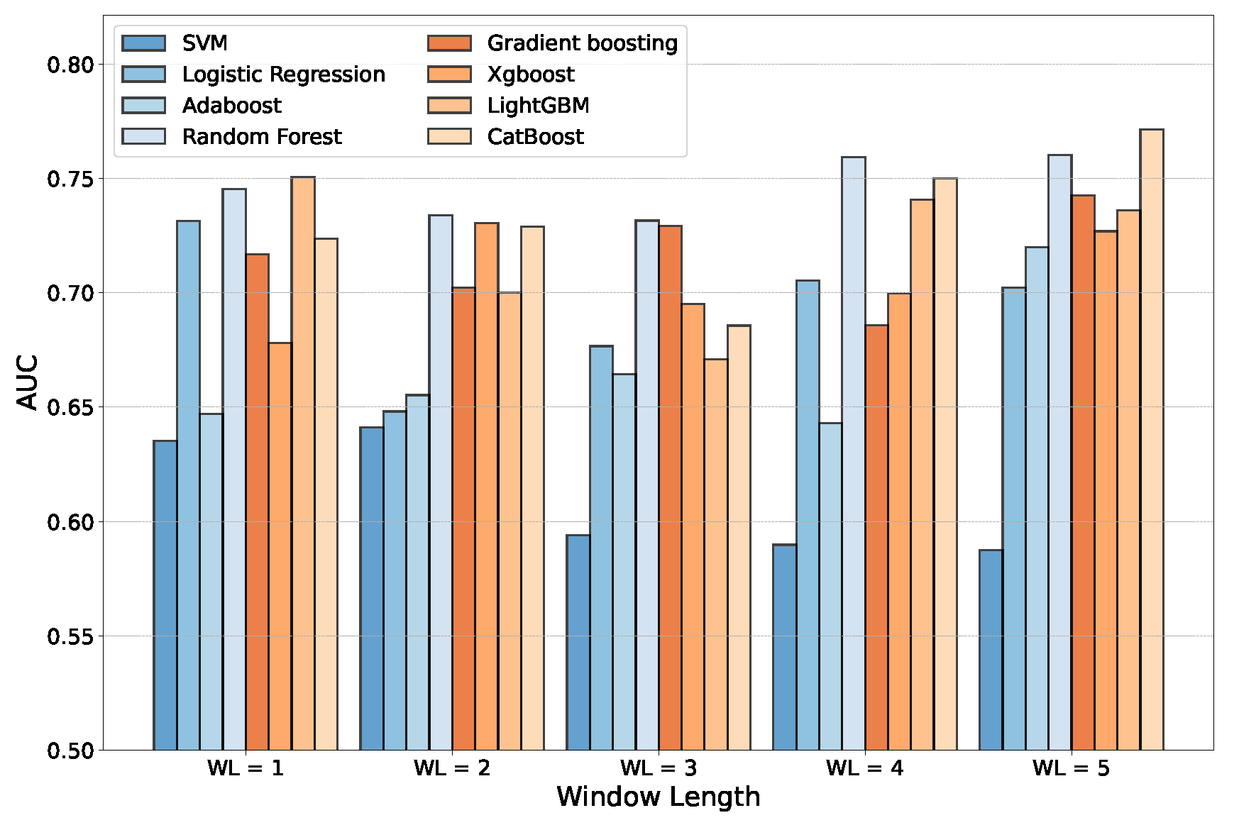
In

Table 3. Average AUC on the validation set depending on the number of years considered (window length, WL). The best results for $WL=4$ and $WL=5$ are highlighted in boldface.

ML Model	Average AUC
	WL = 1	WL = 2	WL = 3	WL = 4	WL = 5
Support Vector Machine	0.635	0.641	0.594	0.589	0.587
Logistic Regression	0.731	0.648	0.676	0.705	0.702
AdaBoost	0.647	0.655	0.664	0.642	0.719
Random Forest	0.745	0.733	0.731	0.759	0.760
Gradient Boosting	0.716	0.702	0.729	0.685	0.742
XGBoost	0.678	0.730	0.695	0.699	0.726
CatBoost	0.724	0.729	0.686	0.749	0.771
LightGBM	0.751	0.699	0.671	0.741	0.736

we report the average results obtained on the validation set for every model depending on the number of years considered (window length, WL). Figure 5 summarizes the comparison. As expected and according to the previous literature, the ensemble models usually reached better results. In particular, we found that for $WL=4$, the Random Forest with 500 estimators obtained, on average, a greater AUC on the validation set. On the other hand, for the $WL=5$ case, the best model found was CatBoost. In both cases, the two ML algorithms achieved better performance compared with the other baselines. For this reason, we considered both CB and RF for the subsequent analysis.

It is important to note that none of the ML models considered were designed to work on time series data, thus they considered all the variables as independent features. As expected, increasing the window length led to a longer training time on average for all the models (

Table 4. Average training time (seconds) on the validation set depending on the window length (WL). Times in seconds refer to the average training time for a single run.

ML Model	Average Training Time (s)
	WL = 1	WL = 2	WL = 3	WL = 4	WL = 5
Support Vector Machine	0.032	0.036	0.036	0.034	0.033
Logistic Regression	0.018	0.022	0.023	0.024	0.026
AdaBoost	0.826	1.246	1.560	1.769	1.994
Random Forest	0.799	0.973	1.033	1.034	1.059
Gradient Boosting	1.022	1.833	2.545	3.097	3.555
XGBoost	0.421	0.422	0.493	0.478	0.483
CatBoost	6.670	7.059	7.088	7.383	7.398
LightGBM	0.187	0.195	0.191	0.184	0.179

). However, all the models required just a few seconds of training with our hardware settings. However, the ensemble models performed better than SVM and LR with more variables and a larger window length. Moreover, using the 18 accounting variables for 4 or 5 consecutive years yielded a better result in terms of AUC, in particular with Random Forest ($0.759$ for $WL=4$) and CatBoost ($0.771$ for $WL=5$). A possible consideration is that although RF and CB showed similar overall performance, the computation time required to train CB was almost six times that required for RF. However, the computation time was not relevant in our experiments since the dataset was not particularly large. In light of this, we selected $WL=4$ and $WL=5$ to further study time series data with Recurrent Neural Networks.

8. LSTM Architectures for Bankruptcy Prediction

According to [43], LSTM performs better than a GRU when the sequence is short, although with a matrix input. For this reason, we chose the LSTM approach for our experiments since we were considering eighteen different time series as input, each with a short sequence length, as determined in the first experiments presented in Section 7. In order to study the application of RNNs to bankruptcy prediction, we evaluated two different architectures:

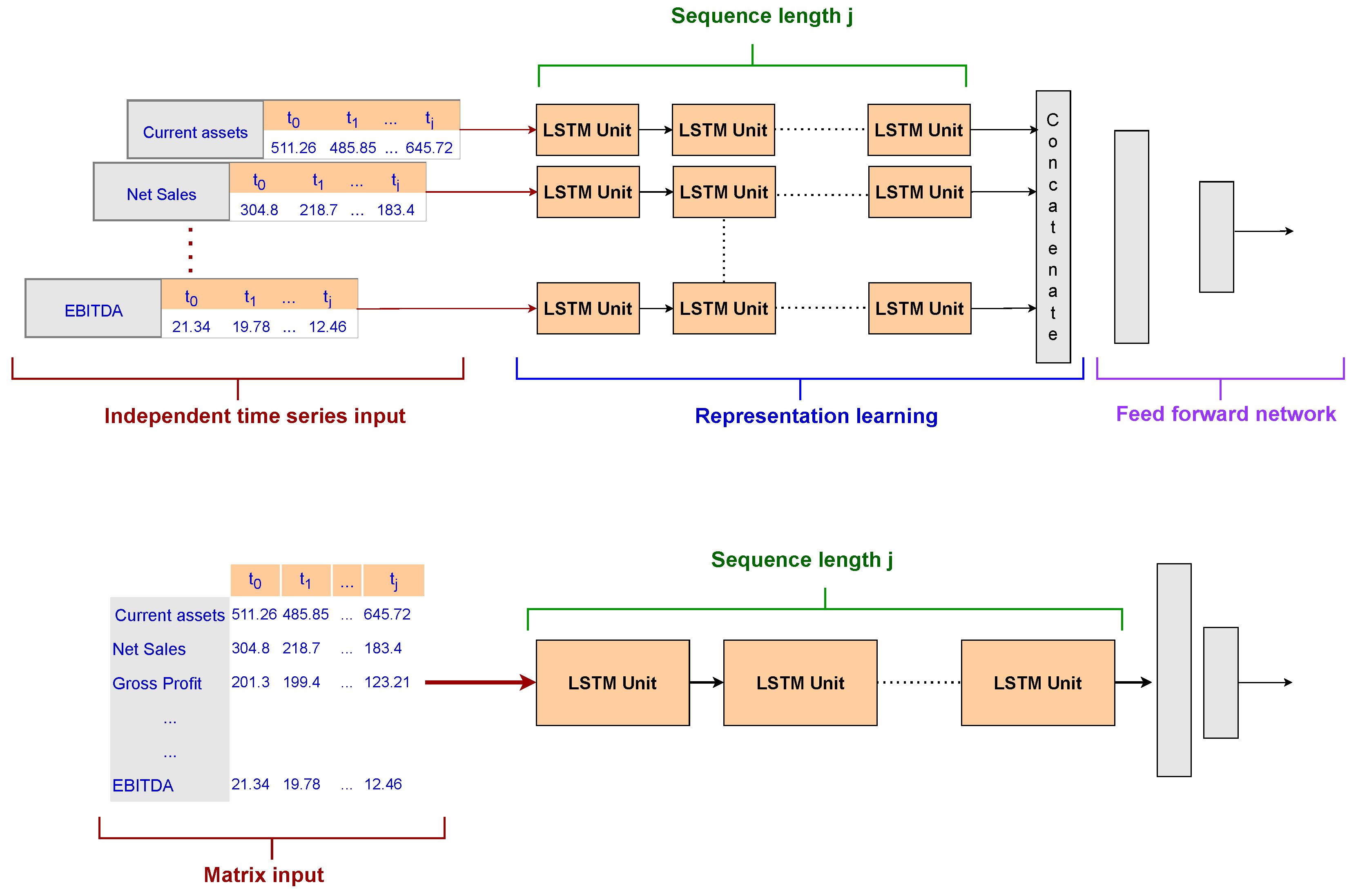
• Single-input LSTM: This is the most common approach with RNNs. The input was a matrix with 18 rows (the number of accounting variables) and a number of columns equal to the time window selected for the experiment. Moreover, the LSTM unit was composed of a sequence of units as long as the time window. Finally, a dense layer with a Softmax function was used as an output layer for the final prediction.
• Multi-head LSTM: This is one of the main contributions of our research concerning the current state of the art. To deal with a smaller training set due to the temporal window selection and the class imbalance, we developed several smaller LSTM architectures, one for each accounting variable to be analyzed by the model, named LSTM heads. Each network included a short sequence of units equal to the input sequence length and contributed to the latent representation of the company learned by utilizing the accounting variables. Indeed, th output of the multi-head layer was then concatenated and exploited by a two-layer feed-forward network with a Softmax function in the output layer. This architecture aimed to test whether an attention method based on a latent representation of the company that focused on each time series independently could outperform a classical RNN setting.

Figure 6 summarizes the main differences between the two architectures. The source code for the multi-head LSTM architecture is publicly available on GitHub (https://github.com/sowide/Multi-head_LSTM_for_bankruptcy-prediction, accessed on 1 February 2024).

9. Results

In this section, we present the results we achieved for bankruptcy prediction using the two RNN architectures presented in Section 8. Firstly, we compare the RNNs with the best model found in the preliminary experiments presented in Section 5 using the validation set (2012–2014), and, finally, we show the results obtained on the previously unseen test set (2015–2018) to assess the generalization ability of our models.

9.1. LSTM Training and Validation

The two LSTM architectures were trained with exactly the same parameters for a fair comparison. The main hyper-parameters were the following:

• Epochs = 1000.
• Learning rate = ${10}^{-4}$.
• Batch size = 32 (default Keras value).

To make sure the results were unaffected by unrelated factors, we chose to keep the parameters of both LSTM architectures the same and only compare the performance differences between them based on architectural differences. Instead of investigating the impact of different settings on the results, we wanted to see how their designs affected their performance. However, it is worth noting that, while both architectures began with comparable parameters, they were independently optimized using the validation set and weight initialization approaches. Moreover, we used the early stopping technique to prevent the network from overfitting, and we employed the validation set to select the hyper-parameters. In particular, to deal with the imbalance in the training set, we performed 500 runs for each LSTM architecture by considering a randomly balanced training set every time.

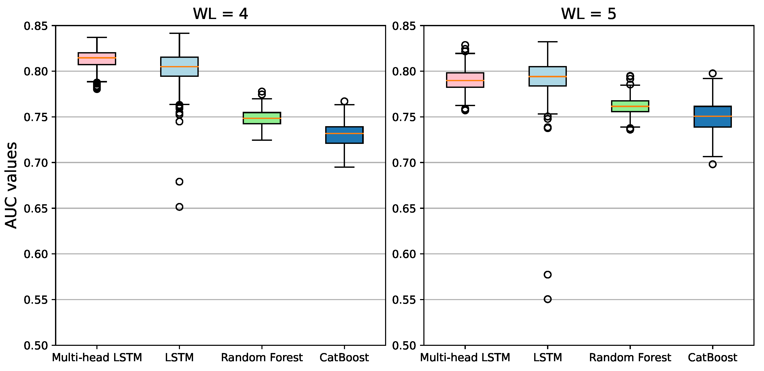
After this, we first compared single-input LSTM, multi-head LSTM, and previous results achieved with Random Forest and CatBoost on the same validation set. Figure 7 shows the model comparison for the temporal windows of 4 and 5 years.

Table 5. Average and max AUC achieved on the validation set (2012–2014) by Random Forest, CatBoost, single-input LSTM and multi-head LSTM. The average training time for each model is also reported for WL = 4 and WL = 5.

	Avg AUC	Max AUC	Avg Training Time (s)	Avg AUC	Max AUC	Avg Training Time (s)
Multi-head LSTM	0.813356	0.837	103.86	0.79	0.828	82.60
LSTM	0.8026	0.8415	51.80	0.7928	0.864	42.86
Random Forest	0.75	0.777	1.035	0.762	0.794	1.062
CatBoost	0.731	0.767	7.388	0.750	0.797	7.432
	WL = 4			WL = 5

summarizes this result in terms of the average AUC achieved in the 500 runs. For each run, the models’ weights were randomly initialized. In light of this result, it is clear that, at least in terms of the AUC, the Recurrent-Network-based deep learning models outperformed traditional classifiers.

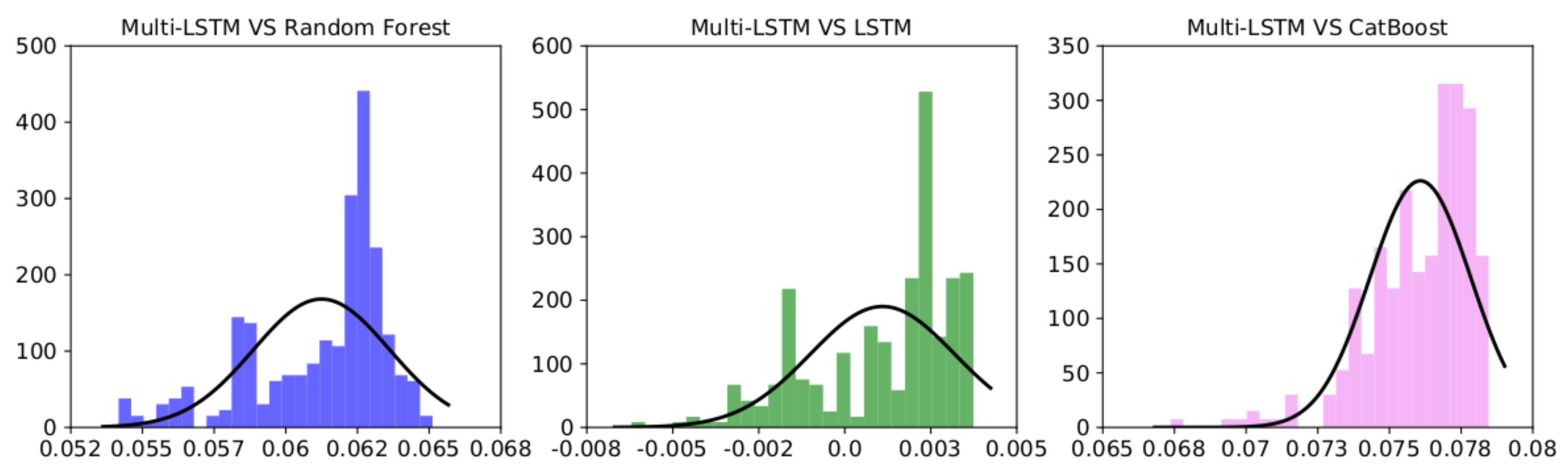
9.2. Statistical Analysis

The experimental results described in the previous section and presented in Table 5 were computed as an average over 500 different runs and show that our model achieved much better AUCs with respect to the other models (LSTM, Random Forest, and CatBoost). We further analyzed these results to prove that our model’s performance was statistically significant. According to [44], a common way to test whether the difference between two classifiers’ results over different datasets or runs is non-random is to compute a paired t-test, which checks whether the difference in their average performance is significantly different from zero.

However, one of the t-test’s requirements is that the differences between the two random variables compared are distributed normally. As we show in Figure 8, none of the performance differences between each model and our multi-head LSTM architecture were normally distributed; for this reason, according to [45], we used the Wilcoxon Signed-Rank (WSR) test ([46]), a non-parametric alternative to the paired t-test that ranks the differences in the performance of two classifiers for each run, ignoring the signs, and compares the ranks for the positive and negative differences. We set to $0.05$ the p-value under which we rejected the null hypothesis (the two distributions had the same median, and thus the performance difference could be considered random).

In our case, we achieved a p-value equal to 0 for each comparison with multi-head LSTM over the same 500 runs when models were trained using the same balanced training set, and the AUC was evaluated over the same unbalanced validation set. In light of these results, we can conclude that our model showed better performance in the period between 2012 and 2014. Finally, since the main goal of this analysis is to build a model that can generalize on unseen samples that were not used during the design phase, we report the next section, our final analysis of the performance of the best models on the test set to better prove the benefits of our approach.

10. Final Analysis on the Test Set

In light of the results achieved on the validation set, we selected the optimal single-input LSTM, the optimal multi-head LSTM, and the optimal Random Forest models. We defined the optimal model as that which met the following three conditions:

• Lowest difference between training and validation loss to ensure that the highest AUC was not achieved as a consequence of overfitting.
• Lowest validation loss.
• Highest AUC on the validation set.

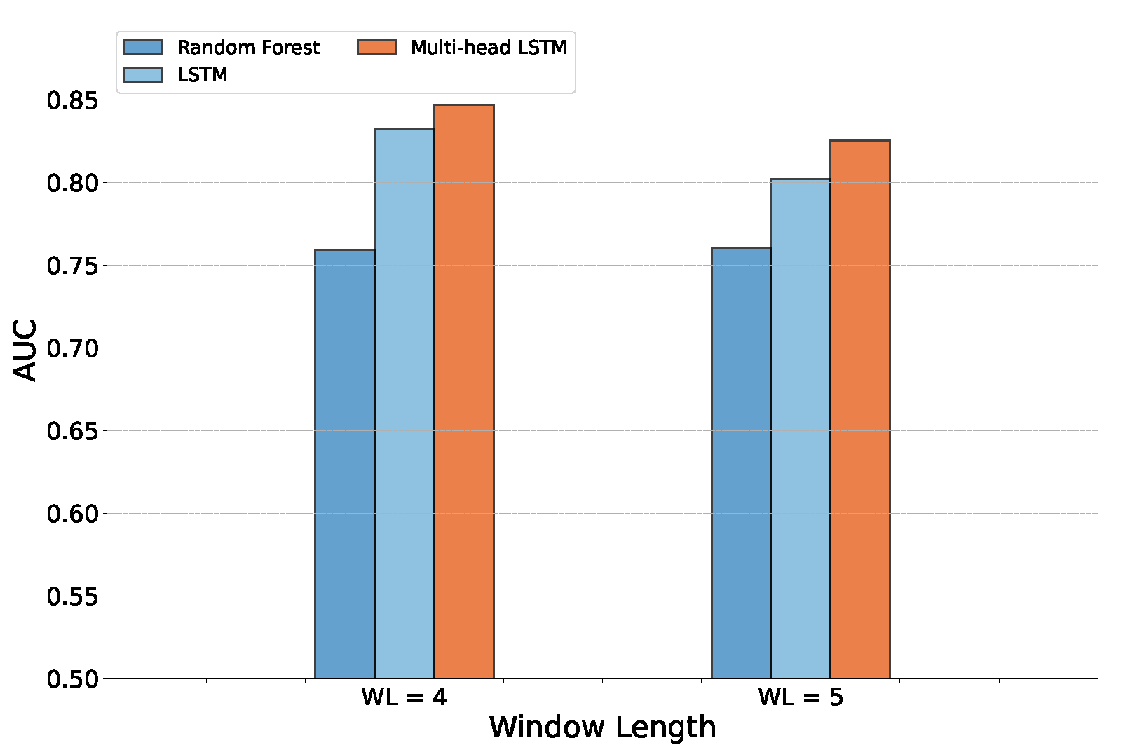
We experimented with the best models on the previously unseen test set (companies between 2015 and 2018). We again compared the single-input LSTM, multi-head LSTM, and Random Forest classifiers. Figure 9 shows the model comparison in terms of AUC. In

Table 6. Overall results on the test set (2015–2018) with single-input LSTM and multi-head LSTM. Rec indicates recall and Pr indicates precision. The best results were achieved for WL = 4 by multi-head LSTM.

	LSTM	Multi-Head LSTM	LSTM	Multi-Head LSTM
TP	88	75	89	71
TN	1233	2158	1071	2085
FN	8	21	2	20
FP	1591	666	1573	559
AUC score	0.832	0.847	0.802	0.825
BAC	0.677	0.773	0.692	0.784
Micro F1	0.772	0.797	0.777	0.793
Macro F1	0.53	0.55	0.528	0.542
Type I error	21.74	18.45	22.65	20.5
Type II error	23.95	28.125	21.97	21.97
Rec bankruptcy	0.76	0.71	0.78	0.78
Pr bankruptcy	0.106	0.117	0.106	0.115
Rec healthy	0.782	0.815	0.773	0.795
Pr healthy	0.989	0.988	0.99	0.99
	WL = 4		WL = 5

, we report detailed results for each model in terms of recall on the bankruptcy class, type I and II errors, and the micro and macro $F_1$ scores. As expected from the previous results obtained for the AUC on the validation set, the best model was still multi-head LSTM, which achieved the best result on the test set. In addition, to gain a deeper insight into our model’s performance on the test set, we leveraged the BAC (balanced accuracy) metric, which is the arithmetic mean of sensitivity and and specificity.

Since the model showed very high precision over the healthy class (Table 6), which was also the majority class in the validation and test sets, the slope differences were probably due to the higher number of correct predictions in the validation set during learning. However, it is possible to observe that no overfitting or underfitting phenomena affected our model, as is also shown by the good results on the unseen test set (Figure 9).

Therefore, we can conclude that RNNs have an impact on bankruptcy prediction performance. However, the attention model induced by multi-head LSTM seemed to achieve better results for all the metrics (AUC and micro and macro $F_1$ scores) with a temporal window equal to 4 years. On the other hand, considering the minimization of the false-negative rate, the models with WL = 5 achieved, in general, the lowest type II errors.

10.1. Further Analysis on the Test Set

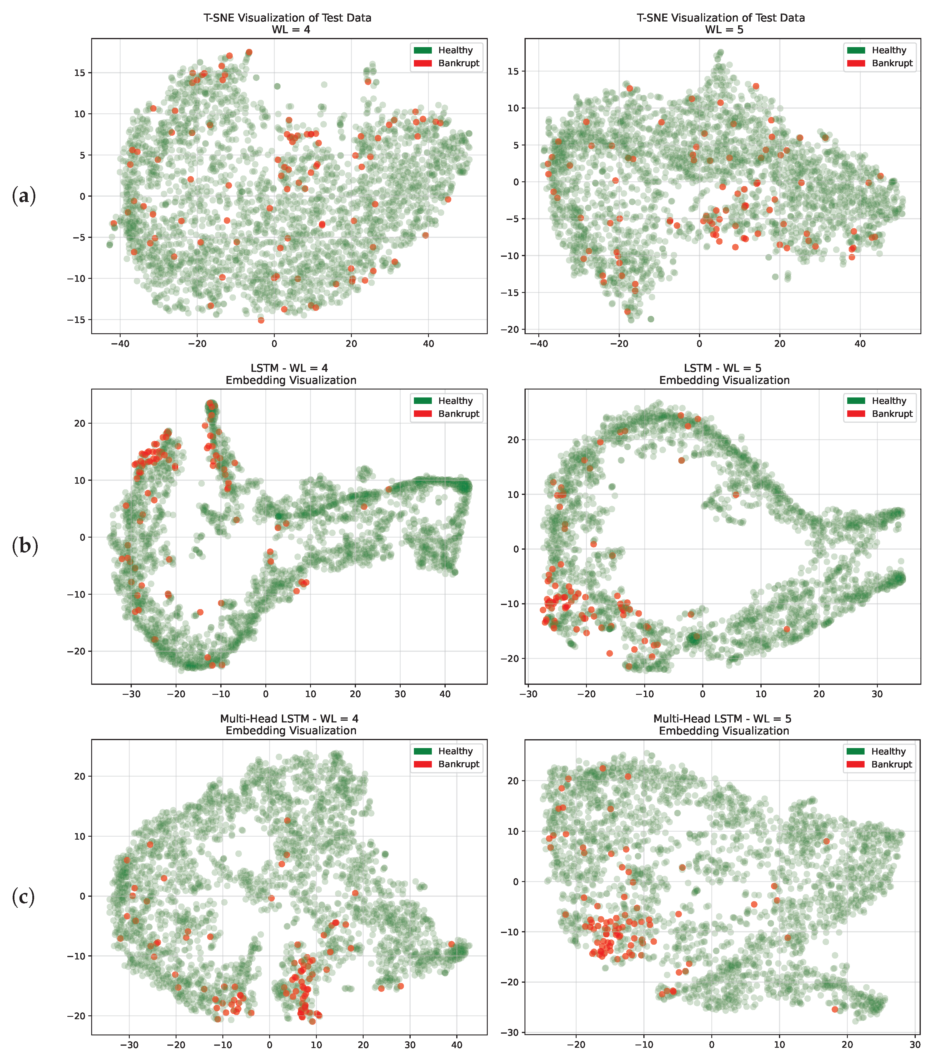
Understanding the distribution and the relationships within the feature space is crucial for gaining insights into the behavior of a model. Among the methodologies employed for representing high-dimensional data, one of the most powerful approaches is t-distributed stochastic neighbor embedding (T-SNE) [13]. T-SNE preserves the non-linear structure of data points and tends to maintain the relative distances between neighboring points, which can reveal clusters and patterns. The analysis reported in this subsection aimed to study the distribution of both healthy and bankrupt firms in a reduced-dimensional space, focusing on the capabilities of multi-head and single-input LSTM in identifying an optimal decision boundary.

We first leveraged T-SNE for the original input to visualize the data in a two-dimensional space while preserving the pairwise similarities between data points. Each data point represented a firm, allowing us to gain an intuitive understanding of its inherent structures. The results are shown in Figure 10a. We performed an analysis using the best window lengths identified on the validation set (WL = 4 and WL = 5). We could infer that bankruptcy-prone firms usually did not cluster in a specific region of the feature space of the input. This observation highlights how challenging it is to classify bankrupt companies because there is some degree of overlap with healthy ones.

Following the outcomes achieved from the T-SNE analysis of the original test set, we focused on how the LSTM networks represented each firm in their latent space before classifying them, as depicted in Figure 10. These snapshots offer some insights into the decision boundaries identified by the two recurrent architectures. The decision boundaries for LSTM are depicted in Figure 10b, and those for multi-head networks in Figure 10c.

Our analysis revealed that these embeddings effectively distributed firms, with bankrupt firms forming distinct clusters. This demonstrates the models’ ability to capture meaningful patterns in the data, particularly concerning bankruptcies. The models consistently demonstrated the ability, whether the window length was equal to 4 or 5, to discriminate between healthy and bankrupt firms in a two-dimensional environment. The models’ constant ability to identify significant patterns linked to financial distress showed their robustness. By comparing the latent representations achieved by single-input LSTM with those achieved by the multi-head model, it was evident that the multi-head model achieved a more scattered representation that led to smaller overlaps between healthy and bankrupt firms. This result is also in line with the results presented in Table 6, checking the number of false positives (FPs) achieved by the two models. Thanks to this, multi-head LSTM outperformed single-input LSTM in terms of AUC, BAC, and FP for both window lengths.

For this reason, we decided to further study the false positives with an additional analysis, as presented in the following section.

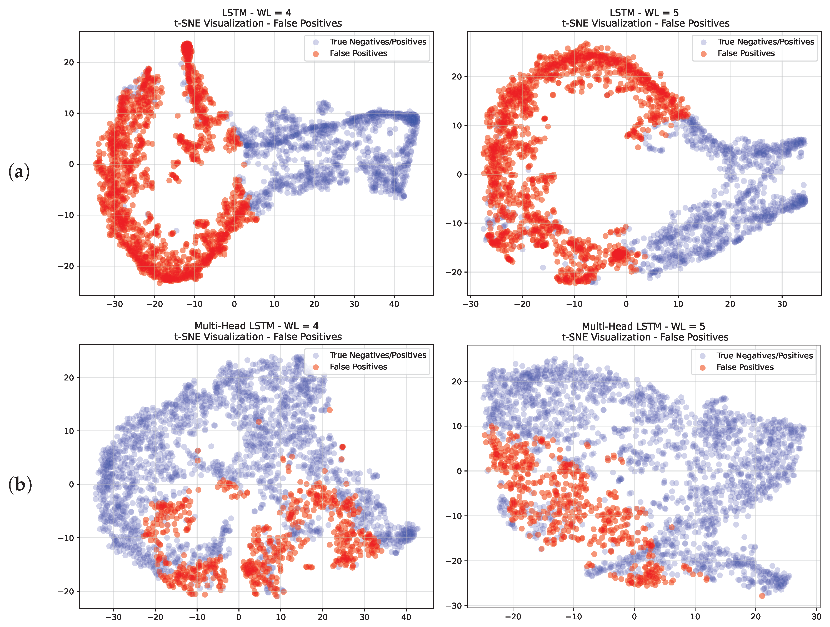
10.2. False-Positive Analysis

In bankruptcy prediction, an error has a different cost depending on the class that has been incorrectly predicted. The cost of predicting a company going into default as healthy (FN) is much higher than the cost of predicting a healthy one as bankrupt (FP). Both networks achieved a small number of false negatives but a considerable number of false positives that affected the performance. Moreover, in light of the evidence presented in the previous section about the different levels of overlap between bankrupt and healthy firms achieved by the multi-head and single-input LSTM models, we decided to further analyze the latent representation (embedding) of the false positives achieved by both networks to better prove the benefits introduced by the multi-head LSTM architecture.

For this analysis, we again leveraged T-SNE dimensionality reduction to display the distribution of false positives. The results are depicted in Figure 11 for window lengths of 4 and 5 years.

Examining the embedding obtained from both models, one may observe how the false positives were close to the bankruptcy clusters presented in the previous section, presenting a considerably smaller overlap ratio with healthy firms in the case of multi-head LSTM.

Furthermore, to complete our analysis, we considered how the false positives were distributed across the financial industries since economic conditions and market dynamics can significantly impact the behavior of businesses within a particular industry. With this aim, we leveraged the SIC codes presented in Section 4 to understand if industry-specific factors can contribute to misclassification.

Table 7. Division distribution in the test set for each model. This table provides an overview of the distribution of companies across various divisions within the test set, including the total number of companies belonging to each category. However, for LSTM and multi-head LSTM models, only instances of false positives are reported, along with their distribution among different divisions. Additionally, percentages are presented to express the ratio of false positives in relation to the total data present in the test set.

Division	Test Set		LSTM (False Positive)		Multi-Head LSTM (False Positive)
	WL = 4	WL = 5	WL = 4	WL = 5	WL = 4	WL = 5
A	17	15	12 (70%)	9 (60%)	4 (23%)	3 (20%)
B	152	142	84 (55%)	79 (52%)	34 (22%)	29 (20%)
C	30	28	13 (43%)	14 (50%)	5 (17%)	6 (21%)
D	1476	1382	824 (55%)	790 (57%)	326 (22%)	284 (21%)
E	254	248	107 (42%)	139 (56%)	77 (30%)	44 (18%)
F	106	99	73 (69%)	71 (72%)	34 (32%)	28 (28%)
G	213	202	134 (62%)	131 (65%)	104 (49%)	95 (47%)
H	66	63	34 (52%)	32 (51%)	12 (6%)	5 (8%)
I	606	556	310 (51%)	308 (55%)	70 (11%)	65 (12%)

presents the false positives for both models across different SIC divisions under different test set conditions (WL = 4 and WL = 5), as well as the respective percentages. We could make the following observations:

• Across all divisions, the multi-head model outperformed LSTM for both window lengths in terms of the number of false positives. This shows how much better multi-head LSTM was in classifying and identifying alive and bankrupt firms.
• Examining the variation in false positives with an emphasis on window length revealed an interesting pattern. When considering multi-head LSTM, the greater the window length, the lower the percentage of false positives. This can be explained by multi-head LSTM’s capacity to identify structures and patterns that could be missed when the window was set to 4 years. Conversely, since single-input LSTM’s performance had more variance, no definitive conclusions could be drawn about it, making it difficult to understand how the false positives changed across various time windows. This is because there were equal numbers of positive and negative variations.

These observations regarding the sectors and spatial distribution of false positives provide important guidance for improving model parameters, maximizing predictive precision, and eventually improving our models’ applicability in bankruptcy prediction tasks.

11. Conclusions

In this paper, we proposed a multi-head LSTM neural network to assess corporate bankruptcy. According to the experimental analysis on the test set, this model outperformed single-input LSTM with the same hyper-parameters and architecture, as well as the other traditional ML models. The better forecasting performance of multi-head LSTM also proved that modeling each accounting time series independently with an Attention head contributes to better-identifying companies that are likely to face default events (highest recall and lowest type II error). This was also evident in the analysis of false positives presented in the experimental section. Moreover, we can finally argue that using accounting data for the four most recent fiscal years leads to better performance when predicting the likelihood of corporate distress. Experiments were conducted on a dataset composed of accounting variables from 8262 different American companies over the period 1999–2018 for a total of 78,682 firm-year observations. This dataset has been made public so that it can be used as a benchmark for future studies. Future developments will involve exploiting textual disclosures from financial reports in conjunction with this model. Moreover, it should be possible to predict defaults only in specific sectors by adding macroeconomic variables such as sustainability, interest rates, sovereign risk, and credit spread. Furthermore, our models provide predictions over a single period, not the survival probabilities over time. In future work, multi-period models can be incorporated to also reach this goal.