Abstract
Numerous applications of the Internet of Things (IoT) feature an event recognition behavior where the established Shannon capacity is not authorized to be the central performance measure. Instead, the identification capacity for such systems is considered to be an alternative metric, and has been developed in the literature. In this paper, we develop deterministic K-identification (DKI) for the binary symmetric channel (BSC) with and without a Hamming weight constraint imposed on the codewords. This channel may be of use for IoT in the context of smart system technologies, where sophisticated communication models can be reduced to a BSC for the aim of studying basic information theoretical properties. We derive inner and outer bounds on the DKI capacity of the BSC when the size of the goal message set K may grow in the codeword length n. As a major observation, we find that, for deterministic encoding, assuming that K grows exponentially in n, i.e., , where is the identification goal rate, then the number of messages that can be accurately identified grows exponentially in n, i.e., , where R is the DKI coding rate. Furthermore, the established inner and outer bound regions reflects impact of the input constraint (Hamming weight) and the channel statistics, i.e., the cross-over probability.
1. Introduction
The Internet of Things (IoT) refers to a system of interconnected devices that communicate and share data with one another [1,2]. The IoT is first-class and the fastest growing area of technology, where its constituent is called a thing. These things are classified in three groups: people, machines and information (food, medicines, books, etc.). Examples include a driving car with built-in sensors monitoring vehicle health and driving performance, or a person with a heart monitor implant for efficient patient management, and can be very varied, including any natural or human-made objects that has sensors, processing/controlling ability, and can transfer information over a network using specific communication technologies. Some of the key challenges and possible research topics for IoT are highlighted in [3]. Moreover, in [4], different physical layer security techniques for IoT are studied.
Smart cities: IoT can be used in the context of smart cities [5], where it provides an urban network to connect devices such as sensors, lights, and meters, for the sake of data collection and analysis. The smart cities exploit state-of-the-art technologies such as cloud computing [6] and machine learning [7] to provide a better quality of government service, enhancing infrastructure, public utilities, and citizen services. In particular, in the context of smart mobility and transportation systems [8], IoT may provide opportunities for integrating control, communications, and date processing across a heterogeneous network of transportation systems. IoT applications can be extended to different aspects of such systems, including the infrastructure, vehicle, and user/driver. The interactions between such components give rise to inter- and intra-vehicular communication, smart traffic control, safety, logistics, user/vehicle control, electronic toll collection systems, etc. [9]. Specifically, a potential IoT application scenario for these contexts is exploiting sensors for the sake of environmental monitoring [10]. That is, in a wireless sensor network, a group of sensors which monitor the environment are expected to send the minimum amount of information to the decision center for the sake of performing an appropriate and reliable timely act.
Smart medical and health-care systems: Applications of IoT for medical and health-care purposes are referred to as the Internet of Medical Things (IoMT) [11,12]. In this context, the technology for creating a digitized healthcare system where the medical resources cooperate with others for providing health-care services is referred to as smart health-care. In particular, IoT devices may be used for enabling remote emergency notification systems and health monitoring. Such devices range from blood pH/pressure and heart rate monitors to more advanced devices capable of monitoring specialized implants, such as pacemakers, wristbands, or sophisticated hearing aids [11]. Moreover, a field related and concurrently expanding to the IoMT is the Internet of Bio-Nano Things (IoBNT) [13,14] which is the application of IoT for connecting bio-nano things inside the human body in order to provide a network of nano-scale and biological devices. A parallel developing and linked field to IoMT and IoBNT is molecular communication (MC), which provides platform, tools and techniques for establishing communications in the molecular scale [15,16].
1.1. Post-Shannon Communications for IoT
The classical information theory was established by Shannon in [17], where three levels of communications, including technical (reliable symbol transmission), semantic (message’s meaning transfer) and effectiveness (achieve goal/pragmatic aspect of message exchange) problems were defined. Shannon, in [17], considered solely the technical problem, which focuses on the accurate transmission of symbols. However, several applications for emerging sixth-generation (6G) or future-generation (XG) wireless communications/networking systems in the context of IoT demand to deal with the semantic and effectiveness aspects of the message. In fact, future XG systems fold the semantic of message and the goal of message communication into their design. This is required in these applications in order to fulfill certain performance features, including sustainability (robustness), latency, reliability, security, etc. Studying these new aspects of the message goes beyond the conventional Shannon paradigm/framework, and are referred to as post-Shannon communications (PSCs) [18]. For example, in goal/task-oriented communications [19], the success of execution for specific task (effectiveness problem) at the destination/receiver is the key concern, and is demanded by the transmitter.
In particular, a first discussion of the PSC for 6G can be found in [18]. The use of PSC for MC is studied in [20], in which the possible capabilities of MC for 6G is discussed for the first time. Also, a detailed discussion of the requirements for tactile internet (which refers to the data transfer in real-time (extremely low latency) in combination with high availability and reliability requirements) and 6G can be found in [21], in which the PSC is introduced to be of particular importance for several key areas of applications for 6G, wherein new communication scenarios, performance requirements and open questions for the PSC are discussed as well. Moreover, the wireless communication systems in 5G and beyond networks, which include reconfigurable intelligent surfaces (RISs) [22], deal with aspects such as localization, synchronization and beamforming design. These aspects in RISs often require use of the semantic metrics rather than the conventional Shannon metrics; cf. [23,24] for further details. Moreover, various applications in the context of smart medical and health-care systems for 6G networks require task accomplishment [20], and are needed to adapt the encoded signal depending to the specific application-driven requirements of the receiver.
1.2. IoT Needs and Impact of the Deterministic K-Identification
The evolving growth and development of technologies for IoT use cases have given rise to several applications where a reliable symbol transmission (the technical problem of Shannon) is less relevant. In particular, the 5G and 6G wireless communications systems in the horizon of IoT are expected to create new applications where the semantic and goal performing aspects of the messages are the key concern. Furthermore, these applications suffer other challenges, such as having difficulty coping with generation of randomness and working with sophisticated random number generators. Also, in some case, a strict criterion on the performance speed for recognition/identification of an event is imposed, or it is needed to deal with an increasing size of the search space. In the following, we expand on such challenges in more detail and suggest the K-identification problem as a promising approach for them.
Semantic and goal-oriented communications: Let us define the K-identification problem considered in this paper as follows: Assume that the message set is , and message i is sent by the transmitter. Furthermore, assume an arbitrary subset of the message set with size K by . In the technical problem setting (symbol transmission), the receiver is interested in determining exactly which message is sent by the transmitter, i.e., to reconstruct the sent message. However, in the K-identification setting, the receiver is only interested in determining whether or not the sent message belongs to the set . In other words, the receiver decided or without stating exactly which message is sent. Note that, in principle, identification should be guaranteed for any goal identification message set of size , regardless of whether these identification message sets are intended for one or different receivers. In the K-identification problem, receiver seeks to perform a specific goal/task if its desired message sent at the transmitter, belongs to a set of K messages. Therefore, this problem may help to deliver the semantic aspects associated with the messages and can be adapted to the goal/task-oriented communications settings. That is, the K-identification problem can be a compelling candidate/answer to the IoT needs for applications defined in the context of PSC. These applications often ignore a reliable transmission of bits/symbols, and instead are alarm-triggered and demand to convey the semantic aspects of the messages. Potential applications of the K-identification problem for IoT systems are considered in [25].
Randomness generation/management: The original problem of K-identification proposed by Ahlswede in [26] considers employing randomness in the encoding module of a communication setup. That is, for each message at the transmitter, a unique distribution is assigned, which associates/maps the message to a codeword. This randomized mechanism for the K-identification problem allows for a remarkable gain in terms of the number of different messages (or/and their semantics/effects) that can be conveyed to the receiver, namely a double exponential behavior for the size of the message set; cf. [26] for details. Although in majority of use cases for IoT applications, such a double exponential behavior demand might be already real and steadily increasing, it has not necessarily been a focus point when launching an IoT device on the market. This occurs mostly because of cost and integration barriers. Specifically, in order to ensure standard realization of distributions in the encoding procedure, a true random number generator (TRNG) [27] should be embedded in IoT devices and utilized. Hardware-based TRNGs are often difficult to launch, manage and maintain for specific use cases [28]. These difficulties can be mitigated by exploiting deterministic codes in the system design for some of the applications. In addition, deterministic codes often have the advantage of simpler implementation, simulation [29,30] and explicit construction [31]. As a result, the deterministic K-identification (DKI) considered in this paper may be regarded a promising solution for several IoT applications that do not comprised randomness in their encoding part.
Performance speed: In the standard identification with deterministic encoding (DI) problem (i.e., ) [32,33], the receiver performs a series of comparisons between a given goal message and each element of the message set (one-to-one comparison). However, in the DKI problem, the receiver is capable of performing a one-to-set comparison, i.e., an inclusion test. In other words, the receiver is searching for a specific message within an arbitrary set of K messages (goal message set), and is able to declare reliably whether or not a specific message which is searching for is included in the goal message set. This feature for the DKI problem may be regarded as an advantage in terms of speed in the set-wise search, compared to the DI for identification-based IoT devices. In the following, we explain from a quantitative perspective that why the one-by-one comparison as made in the DI is slow, and why the simple inclusion test as made in the DKI is fast. In order to evaluate the search performance speed of K-identification against the standard identification, let us define the time complexity that is required in order to exhaust the entire collection of subsets of size K as a metric. Then, observe that the message set with size M has subsets of size K, referred to as the search space. Now, note that the total search space is the power set of the message set, i.e., the set of all subsets of the message set with size . Therefore, ratio of the size of the search space to the size of the power set for the message set, converges exponentially to zero in the message size, M, i.e.,
for and , where the inequality holds by ([34], p. 353), with , being the binary entropy function. On the other hand, for the DI problem the sequence of one-to-one comparisons for the asymptotic codeword lengths, n (i.e., very large message set size) trades a long delay on the receiver’s proficiency with an inverse polynomial order in M. More specifically, the receiver searches for a single message among M different messages; therefore, the ratio of the size of the search space to the size of the whole search space is , which tends to zero for increasing M.
Growing search space: Some of the envisioned IoT applications may need a K-identification task where size of the goal message set has to grow in n. For example, where it is required that the size of the goal message set, K, for which the inclusion test (search in a set) is conducted, remains a fixed percentage order of the size of the message set. Therefore, by growing codeword length, n, which implies a growing size of the message set, the corresponding goal message set also grows. To account for these cases, we consider a generalized identification model, whose parameter can grow exponentially in n. Possible implications of this observation in the context of IoT include locating an malfunctioned server within a network of K web servers; spotting/detecting a faulty node in a local partition of wireless sensor network with size K; and in data mining within the procedure of sorting data, where some algorithms need to know that a desired data are included to which set of element with size K.
1.3. Binary Symmetric Channel
A binary symmetric channel (BSC) in information/coding theory is one of the most well-known and fundamental models for communications channels where the input and output alphabets are binary, i.e., . In this model, each symbol (bit) sent by the transmitter experiences a distortion (flipping); that is, the received symbol (bit) can be flipped with a cross-over probability of , but is otherwise received correctly. In contrast to the simplicity of the BSC, many information theoretical problems related to this model are still being investigated in the literature. For example, studying the behavior of the decoding error probabilities and characterization of them as a function of the codeword length n, in the asymptotic for the entire region of coding rate R, which requires knowing the analytic function of the so-called channel reliability function (CRF) [35], is still unknown. In addition, the error exponents for a binary symmetric channel in several settings are not yet completely characterized; cf. [35,36] for further details. The K-identification problem considered in this work is the most generalized and difficult version of the identification problem [26]; therefore, it is rather evident that studying this topic for a general model may be exceedingly hard. However, we can obtain some insights into the effects of the size of goal messages, K, by restricting our investigations to a basic/simple frame of model, i.e., the BSC. More specifically, such information is a theoretical endeavor dedicated to the basic BSC model, which can be useful in the subsequent aspects.
Upgrade to advanced models: Often, studying an information theoretical problem begins with considering the most basic and simple abstract model. This allows the theorists to develop the required analytical tools and techniques in more straightforward manner and benefit the specific results as guides to the use and analysis of more advanced models. In other words, general/advanced models can often inherit/benefit analytical tools, techniques, and comprehensive steps that have been developed for the basic models. For example, studying the DI problem for a discrete memoryless channel (DMC) [32] was initiated/sparked by an earlier work in the literature for the BSC [33].
Error correction codes and modulation: The simplicity of such a basic model with a binary alphabet often is favorable for an explicit code construction problem or for employing modulation techniques. This advantage facilitates the procedure of cultivating novel coding methods. For example, the widely used polar transmission codes are adopted initially for a binary input memoryless channel [31]. Therefore, the simplicity of the BSC model allows experts to utilize it as a promising candidate for evaluation/analyzing the performance of future error correction DKI codes.
Information theoretical characteristics: Several advanced channel models for IoT applications can be simplified/specialized to a BSC. This allows information theorists to examine basic characteristics of such IoT systems (CRF, error exponent, critical rate, etc.) and acquire decent analytical insights needed for practical aspects such as modulation/detection design and explicit code construction. Therefore, studying the BSC effectively yields/suggest solutions for more advanced problems of IoT [37]. In addition, the BSC model is a useful model for studying network coding, which is an important technique in order to enhance the performance of a communication network [36]. Concrete modern scenarios in IoT systems that include the BSC model are telephone links, radio communication lines [37], implementation of noise aggregation methods for physical layer security [4], decision fusions for multi-route and multi-hop wireless sensor networks [38], and multi-hop networks [39].
1.4. Information Theoretical Analysis of BSC-Based IoT Systems
Theoretical advancements of communication channels for IoT systems modeled by BSC are helpful for characterization of their performance limits, which may be used in related system designs. For example, evaluation of explicitly constructed codes for such applications against such performance limit bounds may provide instructive recommendations/interpretations for the sake of efficient encoding/decoding procedures. In this context, for a given error probability and with no restriction imposed on the codeword length, the Shannon message transmission (TR) capacity of the BSC is studied in [17]. In [40,41,42,43], for a specified codeword length and a fix rate less than the TR capacity, the error probability for the optimal TR code is investigated. The problem of construction of optimum or at least good codes for TR problem with a given rate and codeword length is addressed in [40,44,45,46]. Furthermore, the TR capacity of the BSC is shown to be attained by Bernoulli input with success probability, i.e., [35]. In [41], random linear code for the achievability proof with an exponential decoding search is investigated.
However, in the research that is currently available, the BSC has mostly been studied for the TR problem. On the other hand, in [33], the DI for the BSC without input constraint is studied, where the lower bound on the DI capacity is established. In addition, in [32], the DI for the BSC with input constraint in a generalized context of the channel model, namely, DMCs is addressed and an extensive proof, dedicated for the BSC, was not provided. Based on the author’s information, for the BSC with input constraint, with the exception of this paper’s conference version [47], the ultimate performance limits for the deterministic K-identification (DKI) problem have not yet been examined in the literature.
1.5. Applications of the K-Identification Problem for IoT
The use of PSC for MC systems, whose objective is based on recognition of specific event, is studied in [20,48]. In the vision of IoT, the identities of the things are often required to be verified for each other. This identification task is needed in order to make sure that the things can address and reliably communicate with themselves. Consequently, the identification capacity [49] is the primary relevant quantitative metric in such systems, and the TR capacity [17] may not be the primary performance measure. In particular, for event-recognition, alarm-prompt or object-finding problems, where the receiver aims to recognize the occurrence of a specific event, determine an alarm, or realize the presence of an object, with respect to a set, in terms of a reliable Yes/No final decision, the so-called K-identification capacity [26] is the appropriate metric. For the K-identification problems, the receiver is focused on a subset of size K of the message set, , which is known as the goal message set. The recipient chooses a message at random, and confirms if it is part of the specified goal message set. The error requirements imposed on the associated K-identification codes guarantee that each inclusion test is reliable for every arbitrary choice of the goal message set.
In the context of IoT, specific instances of the K-identification problem may be found in the detection of damaged cells in a memory disk drive, where, e.g., a failure detector wants to know whether or not the corrupted cell is present in a group of cells; in lottery prize events, where, e.g., a person aims to determine whether a winner is among their favorite teams or where people seek to know if a specific lottery number is among their collection of numbers; in smart traffic management, where, e.g., one may be interested in finding to which group/set of streets a goal location belongs to. Additionally, K-identification might be used in health monitoring within the context of smart medical and health-care systems. For example, in a remote surgery [50], where the inclusion of a particular cancer or illness inside a goal group of K-cancers/diseases may be the communication goal. Finally, the K-identification problem may find applications in the generalized identification with decoding problem [26] in various IoT applications. Such a problem is an extension of the K-identification, wherein when the receiver identifies that the message belongs to set , and it also identifies the message itself.
1.6. Contributions
In this paper, we address identification systems whose encoders are deterministic and their receiver is required to conduct the K-identification job, i.e., spotting an object/event/message within a set of goal objects/events/messages with size for some . We assume that the communication over n channel uses are independent of each other, and the noise is additive Bernoulli process. We formulate the problem of DKI over the BSC with and without Hamming weight input constraint. Our primary goal is to study the BSC’s DKI capacity region. This study specifically contributes the subsequent contributions:
- ◊
- Generalized identification model: We examine the BSC, in which the size of the goal message set, K, may scale with the codeword length, n. As a consequence, this model incorporates the DI with , and DKI with constant 1. Therefore, we can confirm whether asymptotic codeword lengths allow for reliable identification, even when the goal message set grows in size, using our suggested generalized model. As far as is known by the authors’ knowledge, no previous research has been conducted on a generalized DKI model in the literature.
- ◊
- Codebook scale: We prove that, for K-identification over the BSC with deterministic encoding, the codebook size grows in n, similarly to that of the DI problem () [32,33] and the TR problem [17] over the same channel, namely exponentially in the codeword length n, i.e., ∼, where R is the DKI coding rate, even when the size of the goal message set grows exponentially in n, i.e., , where is the identification goal rate, and certain functions of the channel statistics and input restrictions set upper bounds on it. This result implies that one can extend the collection of goal messages for identification without compromising the codebook’s scalability.
- ◊
- Capacity formula: We derive inner and outer bounds on the DKI capacity region for constant and growing , for the BSC with and without Hamming weight constraints. Our capacity bounds reflect the impact of the channels statistics, i.e., cross-over probability and the input constraint A in the optimal scale of the codebook size, i.e., . In particular, in the coding procedure, we define a parameter , referred to as the distinction property of the codebook which adjust the Hamming distance property for the constructed codebook. Then, assuming a given codebook distinction, , a channel with asymptotic small cross-over probability (i.e., an almost perfect channel) causes the feasible range for the goal identification rate to shrink; that is, the capability of the BSC for K-identification decreases, which is unfavorable. On the other hand, when the cross-over probability increases and converges to its maximum possible values, i.e., (almost pure noisy channel), then the feasible range for begins to enlarge favorably. This observation can be interpreted as follows: The channel noise can be exploited as an additional inherent source embedded in the communication setting for performing the K-identification task with a larger value of K. This observation is in contrast to previous results for DKI over the slow fading channel [51], or the DI for Gaussian and Poisson channels [32,48,52], where capacity bounds were shown to be independent of the input constraints or the channel parameters. We demonstrate that the suggested upper and lower bounds on attainable rates are independent of K for constant K, whereas they are functions of the goal identification rate for increasing goal message sets.
- ◊
- Technical novelty: To obtain the proposed inner bound on the DKI capacity region, we address the input set imposed by the input constraints, and exploit it for an appropriate ball covering (overlapping balls with identical radius); namely, we consider covering of hyper balls inside a Hamming cube, whose Hamming radius grows in the codeword length n, i.e., ∼, for some upper bounded by a function of the channel statistic. We exploit a greedy construction similar as for the Gilbert bound method. While the radius of the small balls in the DI problem for the Gaussian channel with slow and fast fading [32], tends to zero as , here, the radius similar to the DKI problem for the slow fading channel [51] grows in the codeword length n for asymptotic n. In general, the derivation of lower bound for the BSC is more complicated compared to that for the Gaussian [32] and Poisson channels with/out memory [48,52], and entails exploiting of new analysis and inequalities. Here, the error analysis in the achievability proof requires dealing with several combinatorial arguments and using of bounds on the tail for the cumulative distribution function (CDF) of the Binomial distribution. The DKI problem was recently investigated in [52] for a DTPC with ISI where the size of the ISI taps is assumed to scale as . In contrast to the findings in [52], where the attainable rate region of triple rates for the Poisson channel with memory was derived, here, we study the DKI problem for a memoryless BSC, i.e., , and the attainable rate region of pair rates is established. Furthermore, while the method in the achievability proof of [52] is based on sphere packing, which includes an arrangement of non-overlapping spheres in the feasible input set. Here, we use a rather different approach called sphere/ball covering, which allows for the spheres/ball to overlap with each other. For the derivation of the outer bound on the DKI capacity region, it is assumed that a random series of code with diminishing error probabilities is provided. Then, for such a sequence, we prove that an one-to-one mapping between the message set and the set of the feasible input set (induced by the input constraint) can be established. Unlike the previous upper bound proof for DI over the DMC [32]; here, the proof for corresponding lemma is adopted in order to incorporate relevant set of the goal message sets, appropriately. Moreover, in the converse proof, similarly to [52], the method of proof by contradiction was utilized; that is, assuming that a certain property regarding the distance or number of the codewords is negated, we lead to a contradiction related to the sum of the sort I and sort II error probabilities. However, unlike [52], where a sub-linear function for the size of the goal message set was considered, i.e., , here, our converse entails a faster function, namely .
Notations: We use the subsequent notations throughout this paper: We use symbol ≜ for a definition. Alphabet sets are shown by blackboard bold letters . Random variables (RVs) are indicated by upper case letters . Constants and values (realization) of RVs are specified by lower case letters . Row vectors of size n, i.e., and , are represented by lower case bold symbol x and y. The distribution of a RV X is specified by a probability mass function (pmf) over a finite set . The CDF of a Binomial RV is indicated by . All information quantities and logarithms are in base 2. Symbol represents the set of all consecutive natural numbers from 1 to M. We indicate the modulo two addition operator by ⊕. The number of points for which the corresponding symbols for two sequences, and , are different is known as the Hamming metric (distance), i.e., , where is the Kronecker delta, defined as follows:
The Hamming cube is defined as the set of binary sequences with length n, and is denoted by . The n-dimensional Hamming hyper ball of radius r for integers such that , in the binary alphabet, centered at , is defined as
Specifically, for alphabet , center and radius is given by . The volume of the Hamming hyper ball in the q-ary alphabet is defined as the number of points that lie inside the ball, and is denoted by . The set of whole numbers is denoted by . The q-ary entropy function for positive integer , is defined as . for , is denoted by , and is defined as . Throughout the paper, we denote the BSC with cross-over probability by .
1.7. Organization
This paper is structured as follows. Section 2 provides background information on the identification and K-identification problems, and reviews previous results on them. In Section 3, system model and fundamental definitions are established, and the background knowledge about DKI codes are provided. Section 4 introduces our primary results and contributions for the DKI capacity of the BSC. In the end, Section 5 include a summary and possible directions for more research.
2. Background on the Identification Problem
In the subsequent section, we give the background for the current work and establish the identification problem. Also, we motivate for the deterministic-encoder identification versus the well-known randomized-encoder identification (RI) scheme. In addition, we review relevant previous results on the DI, RI, DKI, and randomized K-identification (RKI) capacities for different channels.
2.1. Identification Problem
In the Shannon communication problem [17], a sender encodes its message in a manner that the receiver can perform a reliable reconstruction. That is, the receiver is interested in knowing which message was sent from the transmitter. In contrast, the coding design for the identification setting [49] is intended to conduct a different goal, namely to find out if a desired message was sent by the transmitter or not. Furthermore, we assume that prior to the communication, the transmitter is not informed of the message that the receiver seeks to identify.
Randomized identification: The identification problem (which has been studied in various setting of deterministic or randomized protocols, in the context of communication complexity; see [53,54]) in communication theory is initiated by Ahlswede and Dueck in [49], where a randomized encoder is employed to select the codewords. In this problem, the codewords are chosen based on their corresponding distribution, and the codebook size grows double-exponentially in the codeword length n, i.e., ∼ [49], where R is the coding rate. This observation stands different from the TR problem, where the size growth for the codebook is only exponentially with the codeword length, i.e., ∼. The realization of explicitly constructed RI codes features high complexity, and is often challenging for the applications of MC in the context of IoBNT; cf. [48] for further details. However, in [55,56], explicit construction of RI codes using algebraic codes (Reed-Solomon) has been considered.
Deterministic identification: Although the remarkable properties of RI schemes for the codebook size may seem appealing for some applications, in several practical settings, using a huge amount of randomness may not be favorable. Examples include MC, where implementation in the nano-scaled environment is prohibitive [51], or in a pessimistic jamming scenario, where it is assumed that the radar jammer has access to the whole codebook [57]; therefore, using randomness results in extra expenses and does not guarantee a benefit. Additionally, deterministic codes typically offer advantages such as ease of implementation, simulation experimentation [29,30], and systematic construction [31]. The motivation of Ahlswede and Dueck to develop the RI problem [49] is probably traced back to the work of JáJá [33], who considered DI from a communication complexity perspective (an important observation regarding the behavior of the identification function has been well studied in communication complexity, where the out-performance of randomized protocols over the deterministic protocols (exponential gap between the two classes) for computing such a function is established; for instance, while the error-free deterministic complexity of the identification function is lower bounded by , where m is the length of message, for the randomized protocol and when error is allowed in computation of the identification function, only bits suffices; see [54,58] for further details); that is, where the codewords are determined by a deterministic function from the messages. Moreover, it seems that Ahlswede and Dueck were inspired to show that employing randomness similar to what has been accomplished in the communication complexity field yields an advantage of exponential gap compared to the DI problem (a detailed comparison of codebook sizes in DI and RI problem over various channel models can be found in [48]) for the codebook size. In application cases where complexity is restricted, DI could be preferred over RI. For instance, in MC systems, where the development and deploying of a huge number of random sources (distributions) may not be clear.
K-identification scenario: In the standard DI or RI problems [32,49], the receiver aims to identify the occurrence of a single message, that is, the decoder at the receiver selects an arbitrary message from the message set referred to as the goal message, and then, by exploiting a decision rule (decoder), determines reliably whether or not this goal message is identical to the sent message. The identification problem can be extended in the subsequent sense: The receiver chooses a subset of K messages from the message set, called the goal message set (denoted by ) and, unlike the standard DI or RI problems, it checks whether or not the sent message is a member of . This problem is called K-identification in the literature [26]. The goal message set selected by the receiver can be any arbitrary subset of the message set of size K, among the total such subsets.
The K-identification framework can be thought of as a generalization of DI or RI problems, in which the receiver’s single goal message is replaced with a collection of K goal messages, where . Therefore, the DKI for the special case where corresponds to the DI problem studied in [48,59]. Moreover, the K-identification problem is extended in [26] to generalized identification with decoding, where when the receiver identifies that the message belongs to set , it also identifies the message itself. The K-identification problem, as considered in this paper, is different from a similar scheme called multiple object identification [60], where the sender’s data contains the information of K messages and the receiver’s objective is to identify whether or not a specific message belongs to set . Here, it is assumed that the receiver does not know the set of objects selected by the sender.
2.2. Previous Results on DI Capacity
The DI problem for DMCs subject to an average constraint, is studied in [32] and a full characterization of capacity is established. Therein, the codebook size similar to that of the TR problem [17], is shown to grow exponentially in the codeword length, i.e., ∼ [32]. Ahlswede and Cai studied the DI problem for the compound channels in [57]. Furthermore, recent observation for DI over continuous input alphabet channels including Gaussian channels with fast and slow fading [32], memoryless discrete-time Poisson channel (DTPC) [48], DTPC with inter-symbol interference (ISI) [52], and Binomial channel [59], revealed a new observation regarding the codebook size, namely, it scales super-exponentially in the codeword length, i.e., ∼, which is different than the standard exponential [32] and double exponential [49] behavior for DI and RI problems, respectively.
2.3. Previous Results on DKI Capacity
Ahlswede studied RKI for DMC in ([26] Th. 1), and showed that assuming , the set of all attainable pairs , where R is the RKI coding rate and is the goal identification rate, contains
where is the TR capacity of the DMC. The DKI problem for the slow fading channels, denoted by , in the presence of an average power constraint and assuming a codebook size of super-exponential scale, i.e., , is studied in [51], and the subsequent bounds on the DKI capacity are established:
for . As far as we know, there has not yet been any research performed in the literature on the DKI capacity of the BSC with input constraint, which is pertinent to IoT systems; hence, it is the primary emphasis of this study.
3. System Model and Preliminaries
This section presents the selected system model, and some preliminaries regarding DKI coding are established.
3.1. System Model
We target a communication setting, which is focused on the identification goal; that is, the objective of the decoder is defined as follows: Determine if the sent message belongs to a goal group of messages of size K. In order to do this, the transmitter and the receiver build (the suggested inner and outer bounds on the DKI capacity region functions, whether or not a particular code is utilized for the communication; however, in order to approach the capacity limits, appropriate, explicitly built codes could be needed), a coded communication channel over n, uses of the binary symmetric channel. We assume that the random variables (RVs) and indicate model the input and output of the channel. Each binary input symbol is flipped with probability ; see Figure 1. The stochastic flipping (the extreme cases of or result in and , respectively; hence, these cases are commonly excluded from the analysis) of the input symbol is modeled via an additive binary Bernoulli noise, i.e., . Therefore, the input–output relation of channel reads: , where ⊕ indicate the modulo two addition. That is, the channel input/output are related as follows:
for all and .
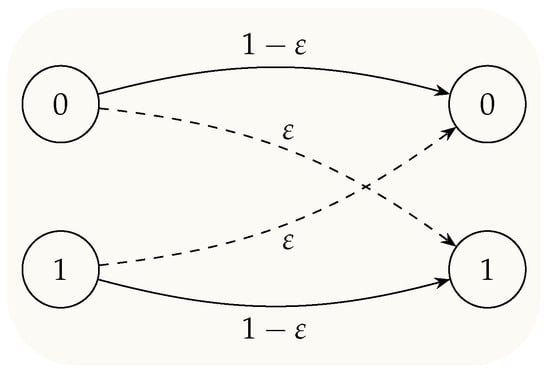
Figure 1.
Bit transition graph over a BSC. Each bit is flipped independently of other bits, with a cross-over probability of .
Furthermore, it is assumed that the various channel uses are independent of one another and that the communication channel is memoryless. Therefore, the transition probability distribution for n channel uses is given by
where and stand for the sent codeword and received signal, respectively, and denotes the Hamming distance. Observe that is a RV, and follows a Binomial distribution; see Remark 1. We assume that the codewords are restricted by an input constraint of the form , where constrain the Hamming weight over the entire n channel uses in each codeword normalized by the codeword length.
Memoryless property: In the standard modeling of the BSC, we assume that the channel is exploited at different time instances in an independent manner; that is, the communications of symbols at distinct time instances are statistically independent of each other. However, in the physical channels, such as telephone lines with impulse noise or slowly fading radio communications with binary alphabet, communication is usually dispersive and the channel exhibit memory [35,61]. Therefore, appropriate steps need to be take in order to ensure the orthogonality of the different channel uses. Some immediate approaches include applying interlacing or scrambling the symbols of a codeword; cf. [61] for further details. Therefore, in the analysis, we can assume that such methods can be applied to circumvent the effect of channel memory and assert statistical independence between different channel noise samples to ensure the memoryless property.
3.2. DKI Coding for the BSC
The definition of a DKI code for the BSC, , is given below.
Definition 1
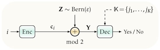
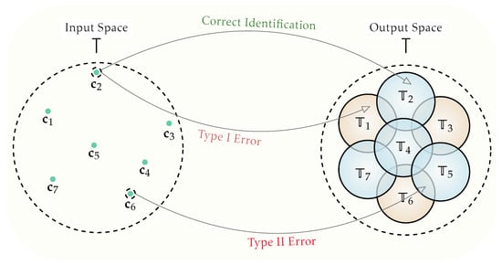
(BSC DKI Code). An -BSC-DKI code for a BSC for integers and , where n and R are the codeword length and coding rate, respectively, is defined as a system , which consists of a codebook , with , such that and a decoder (We recall that the decoding sets for the DKI problem, similarly to that for the RI problem, may have in general intersection; however, to guarantee a vanishing sort II error probability for the asymptotic codeword lengths n, an optimal decoder may be defined in a way such that the size of such intersection regions becomes negligible) , where is an arbitrary subset (recall that the system (family) of all subsets of the set , of size K, is ; note that , and the error requirements, required by the DKI code definition, apply to every possible choice of the set with K arbitrary messages among all cases) of with size K, see Figure 2 and Figure 3.
Figure 2.
System model for DKI communication setting over a BSC. Employing a deterministic encoder at the transmitter, the message i is mapped to the codeword using a deterministic function. The decoder at the receiver is provided with an arbitrary goal message set K, and given the channel output , it asks whether or not i belongs to .
Figure 3.
A DKI configuration with and a goal message set is displayed. The channel’s output is located in the union of each individual decoder (marked in blue) in the correct identification event, where j is a member of the goal message set. If the channel output is seen in the complement of the union of distinct decoders that the codeword’s index belongs to, a sort I error event takes place. When the transmitted codeword’s index does not not belong to , and the channel output is recognized in the union of the individual decoders , with , an error event of sort II occurs.
The encoder sends codeword , given a message , and the decoder’s job is to solve a binary hypothesis: was a goal message that was sent or not? See Figure 3. There exist two sorts of errors that may happen:
- ◊
- Sort I Error Event: Rejection of the actual message; .
- ◊
- Sort II Error Event: Acceptance of a wrong message; .
The associated error probabilities of the DKI code read
where, for every , fulfill the bounds and , where is an arbitrary subset of with size K.
Definition 2
(DKI Coding/Goal Identification Rates). The codebook size and the goal message set size are sequences of non-decreasing monotonically functions in the codeword length n, with , and l indicating the DKI coding rate and the goal identification rate, respectively. In this work, we consider the subsequent functions:
Thereby, the DKI coding rate, R, and the goal identification rate, κ, are defined as follows (additionally, in the literature, other rate definitions for different communication settings are adopted; for example, in the RI [49] problem, the RI coding rate is defined as , while in the TR [17] or DI [32] problems for a DMC, the TR and DI coding rates are given by .):
Definition 3
(Attainable Rate Region). The pair of rates is called attainable if, for every and sufficiently large n, there exists an -BSC-DKI code. Then, the set of all attainable rate pairs is referred to as the attainable rate region for the BSC, , and is denoted by .
Definition 4
(Capacity Region/Capacity). The operational DKI capacity region of the BSC, , is defined as the closure of all attainable rate triples (the closure of a set consists of all points in together with all limit points of , where the limit point of is a point x that can be approximated by the points of ; see [62] for further details), and is denoted by . For the standard identification (), the capacity region is specialized to a single point, also called the DI capacity which is the supremum of all attainable DI coding rates, R. The DI capacity is denoted by .
Remark 1
(Distribution of Output Statistics). Assuming that the codeword is sent and the channel output y is observed at the receiver, the number of cross-overs (flips) that occurs in the channel is given by . Therefore, the probability that k cross-overs among the n channel uses occurs, follows a Binomial distribution with parameters n and ε as follows:
4. DKI Capacity Region of the BSC
In this section, we first present our main results, i.e., the inner and outer bounds on the attainable rates region for . Subsequently, we provide the detailed proofs.
4.1. Main Results
Our DKI capacity region theorem for the BSC, , is stated below.
Theorem 1.
Let indicate a BSC with cross-over probability , and let be an arbitrary constant, where . Further, let indicate the binary entropy function and the tangent line of in point ε be specified as follows:
Next, assume that endows an exponential size for the codebook and the goal message set, i.e., and , respectively, where the codewords are subject to the Hamming weight constraint of the form . Now, let us define the subsequent functions:
Next, let us define the inner and outer rate regions, i.e., and , respectively, as follows:
where
with
and
Then, the DKI capacity region is bounded by
Proof of Theorem 1.
The proof of Theorem 1 comprises two components, presented in Section 4.2 and Section 4.3, respectively, which are the inner and the outer bound proofs. □
Corollary 1
(DI Capacity of The BSC). The inner and outer bounds for the DKI capacity region of the BSC, , for an extreme case (standard identification) where the goal message set consists of only one message, i.e., , recover the previous results for the BSC with Hamming constraint ([32] Ex. 1):
and the BSC without Hamming constraint ([33] Th. 3.1):
Proof.
The proof is obtained directly by placing into the upper bounds given in (17) and (18) in Theorem 1, and making further mathematical simplifications. In particular, we show that closure of the inner bound for coincides the outer bound. Therefore, a full characterization of the capacity region is yielded. We begin with the subsequent observation: The upper bounds provided in (17) and (18) for tend to zero. That is,
where
Next, observe that the outer bound provided in (19) for is given by
which is the closure of the inner bound. Therefore, since the closure of the inner bound region calculated in (24) coincides with the outer bound region given in (25), we obtain a closed form formula for the DI capacity of the BSC as follows:
where there is a Hamming constraint, and
where there is no Hamming constraint. This concludes the proof of Corollary 1. □
Proof.
The proof of Theorem 1 comprises two components, presented in Section 4.2 and Section 4.3, respectively, which are the achievability and converse proofs. □
Here, we summarize some key findings from the proof of Theorem 1.
- ◊
- Input constraint: Theorem 1 reveals an important observation regarding the impact of the input constraint (when it is effective, i.e., ) on the inner and outer regions formulas for the DKI capacity. In contrast to previous results for DI over Gaussian channel [32] or DKI over slow fading channel [51], where the capacity bounds does not reflect the impact of the input constraint, our results for DKI over the BSC in this paper reflect the impact of the Hamming weight constraint on the inner and outer regions.
- ◊
- Scale of codebook: The inner and outer bounds on the DKI capacity region given in Theorem 1 are valid in the standard scale for the codebook size, i.e., , where R is the coding rate. This result coincides the conventional behavior of the codebook size for TR [17] and DI [32] problems over the BSC. Other scales higher than the exponential for the codebook size of K-identification problem are reported in the literature; see Figure 4.
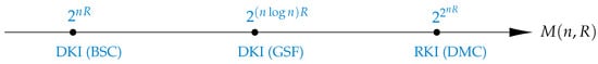 Figure 4. Range of codebook sizes for various K-identification configurations. The codebook scale for DKI problem over the BSC coincide the conventional exponential behavior. But, aside from the standard exponential and double exponential code sizes [26] (RKI over DMC), a different non-standard codebook size is also observed for Gaussian channel with slow fading (GSF); namely, it grows super-exponentially in the codeword length n, i.e., .
 - ◊
- Scale of goal message set: Theorem 1 unveils that the size of the set of the goal messages scales exponentially in the codeword length, i.e., ∼. In particular, the result in Theorem 1 about size of the goal message set constitutes of the subsequent three cases in terms of K:
- DI, : In this scenario, the goal message set is a degenerate case; that is, , with , and is equivalent to the standard identification setup (), where . As a result, the identification setup in randomized regimes [49] and deterministic regimes [32] can be thought of as a particular instance of the K-identification that is examined in this work. See Corollary 1 for further details.
- Constant : The scenario where as is implied by a constant . Our capacity bounds in Theorem 1 on the attainable rate pairs are the same as those for . That is, the result in this cases converge to those for given in Corollary 1, for the asymptotic .
- Growing K: The fact that a trustworthy K-identification is still attainable, even in cases where K scales with the codeword length as ∼ for some , is another significant finding of Theorem 1 ; see Figure 5.
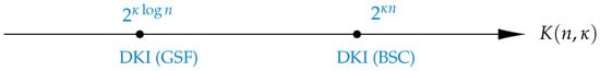 Figure 5. Spectrum of goal message set sizes for different K-identification setups. The goal message set scale for DKI problem over the BSC grows exponentially in the codeword length. Additionally, the GSF channel represent a sub-linear scale, which is lower than the conventional exponential behavior. The scale of goal message set for the BSC is identical to its codebook scale, i.e., exponentially in the codeword length.
We provide the inner bound proof in Section 4.2 and the outer bound proof in Section 4.3 as the proof of Theorem 1.
4.2. Inner Bound (Achievability Proof)
Before we provide the inner bound proof, we explain on our methodological approaches that are used here and expand on them. In particular, similar to other information theoretical problems, the derivation of the inner bound on the DKI capacity region, consists of the subsequent two main steps:
- ◊
- Step 1 (rate analysis): First, we propose a greedy-wise method for codebook construction, which has a flavor similar to that observed in the classical approach of the Gilbert–Varshamov (GV) bound (the early introduction of such a bound in the literature is accomplished by Gilbert in [63]) for covering of overlapping balls embedded in the input set. More specifically, we introduce a codebook of exponential size in the codeword length n, which fulfills the input constraint and enjoys a Hamming distance property; namely, every pair of distinct codewords are separated by a certain distance. Moreover, we introduced a parameter in order to account/adjust such a distance. This step is particularly relevant in the sort II error analysis, as well as the derivation for the final lower bound on the identification coding rate. Additionally, we identify the whole range across which the parameter can change, which is needed to derive an analytical lower bound on the corresponding codebook size.
- ◊
- Step 2 (error analysis): In the second part (error analysis), we show that the suggested codebook in the previous part is optimal, i.e., leads to an attainable rate pairs . To this end, we begin with introducing a decision rule which is a distance decoder based on the Hamming metric, and would show that the associated errors of the sort I and the II probabilities vanish in the asymptotic codeword length, i.e., when . Moreover, the error analysis for the sort II error probability determines the associated error exponent. As a result, the feasible region for the goal identification rate is obtained.

In the following, we confine ourselves to codewords that meet the subsequent condition: , . Furthermore, we divide them into two cases:
- ◊
- Case 1—with Hamming weight constraint: , then the condition is non-trivial in the sense that it induces a strict subset of the entire input set . We denote such subset by and is equivalent to .
- ◊
- Case 2—without Hamming weight constraint: , then each codeword belonging to the n-dimensional Hamming cube fulfilled the Hamming weight constraint, since . Therefore, we address the entire input set as the possible set of codewords and attempt to exhaust it in a brute-force manner in the asymptotic, i.e., as .

Observe that, within this case, we again divide into two cases:
- .
- .
The argument for the need of such division is that the binary entropy function is monotonic increasing in domain and decreasing in domain . In the latter case, we can introduce an alternative Bernoulli process, which results in a larger volume space, and at the same time, it guarantees the Hamming weight constraint.
For the sub-case 1, i.e., where , we restrict our considerations to an n-dimensional Hamming hyper ball with edge length A. We use a packing arrangement of overlapping hyper balls of radius in an n-dimensional Hamming hyper ball .
Lemma 1
(Space exhaustion). Let and let be an arbitrary positive constant referred to as the distinction property of the casebook.
Then, for sufficiently large codeword length n, there exists a codebook , with , which consists of M sequences in the n-dimensional Hamming hyper ball , such that the subsequent holds:
- ◊
- Hamming distance property: , where .
- ◊
- Codebook size: the codebook size is at least .
Proof.
Recall that the minimum Hamming distance of a code is given by
We begin to obtain some codewords that fulfill the Hamming weight constraint, namely,
First, we generate a codeword (such a random generation should not be confused with a similar procedure as is accomplished in the encoding stage of the RI problem. While therein, each message is mapped to a codeword through a random distribution, here for the DI problem, we first solely restrict ourselves to generation of codewords through the Bernoulli distribution to guarantee the Hamming weight constraint, and employ them in the next procedure called the greedy construction up to an exhaustion. Then, after the exhaustion, we establish a deterministic mapping between the message set and the codebook; that is, each message is associated with a codeword. Further, in the RI problem, it is in general possible that two different messages are mapped to a common codeword; however, considering the DKI problem in here, there exists a one-to-one mapping between the set of messages and the set of codewords). Since , by the weak law of large numbers, we obtain
where is an arbitrary small positive. Therefore, for sufficiently large codeword length n, the event occurs with probability 1, which implies that, for sufficiently large n, the subsequent event happens with probability one:
Now, observe that since (31) holds for arbitrary values of , it implies that the subsequent condition for sufficiently large n, is fulfilled
which is the Hamming weight constraint, as required.
Next, we begin with the greedy procedure as follows: Let us denote the first codeword determined by the Bernoulli distribution by , and assign it to message with index 1. Then, we remove all the sequences that have a Hamming distance of less or equal than from . That is, we delete all the codewords that lie inside the Hamming ball with center and radius . Then, we generate a second codeword by the Bernoulli distribution, and repeat this procedure until all the sequences belonging to the feasible subspace, i.e., the Hamming hyper ball, , are exhausted. Therefore, such a construction fulfills the property provided in Lemma 1 regarding the minimum Hamming distance of the code, i.e.,
In general, the volume of a Hamming ball of radius r, assuming that the alphabet size is q, is the number of codewords that it encompasses, and is given by ([64] see Ch. 1)
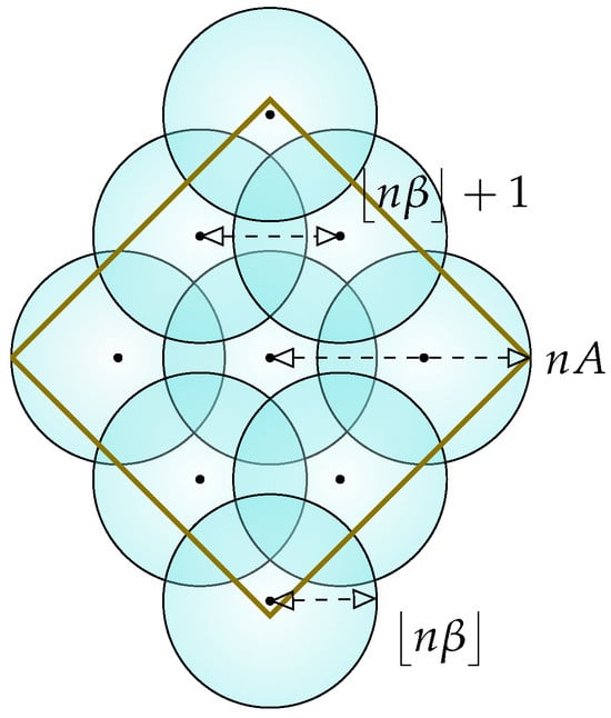
Let denote the obtained ball covering after the exhaustion of the entire Hamming hyper ball , i.e., an arrangement of M overlapping small hyper balls , with radius where , that cover the entire Hamming hyper ball, , where their centers are coordinated inside the , and the distance between the closest centers is ; see Figure 6. As opposed to the standard ball packing observed in coding techniques [65], the balls here are neither necessarily entirely contained within the Hamming hyper ball, nor disjoint. That is, we only require that the centers of the balls are inside and have a non-empty intersection with , which is rather a ball covering problem.
Figure 6.
Illustration of an exhausted greedy-wise ball covering of an n-dimensional Hamming hyper ball , where the union of the small balls of radius cover a larger Hamming hyper ball. As the codewords are assigned to the center of each ball lying inside the an n-dimensional Hamming hyper ball according to the greedy construction, the Hamming weight of a codeword is bounded by , as required.
Th ball covering is called exhausted if no point within the input set, , remains as an isolated point; that is, with the property that it does not belong to at least one of the small Hamming hyper balls. In particular, we use a covering argument that has a similar flavor as that observed in the GV bound ([66] Th. 5.1.7). Specifically, consider an exhausted packing arrangement of
balls with radius embedded within the space . According to the greedy construction, the center of each small Hamming hyper ball, corresponds to a codeword. Since the volume of each hyper ball is equal to , the centers of all balls lie inside the space , and the Hamming hyper balls overlap with each other, the total number of balls is bounded from below by
where holds since the Hamming hyper balls may have in general intersection, and follows by (34) with setting , since . Now, the bound in (36) can be further simplified as follows:
where exploits Lemma (A66) for setting radius and , and (A76) with . Now, we obtain
where the dominant term has an order of n. Therefore, in order to obtain finite value for the lower bound on the DKI coding rate, R, (38) induces the scaling law of codebook size, M, to be . Hence, we obtain
which tends to as .
Now, we proceed to the sub-case 2, i.e., where . In this case, instead of sticking to generation of codewords , we generate the codewords according to Bernoulli process with success probability of ; that is, . Observe that the required Hamming weight constraint given in (29) is now met, since for , we have
Therefore, subsequent similar line of arguments as provided for the sub-case 1, we obtain the subsequent lower bound on the DKI coding rate, R,
which tends to as . □

Lemma 2
(see [33], Claim 1). Let , and let be an arbitrary positive constant referred to as the distinction property of the casebook. Then, the entire Hamming cube can be exhausted for the codebook in the asymptotic codeword length n, i.e., where . That is, for a sufficiently large n, we obtain , with , which consists of M sequences in the n-dimensional Hamming hyper ball , such that the subsequent holds:
- ◊
- Hamming distance property: For every , where , we have
- ◊
- Codebook size: The codebook size is at least .
Proof.
Recall that the minimum Hamming distance of a code is given by
Next, we begin with the greedy procedure as follows: Let us denote the first codeword determined by the Bernoulli distribution by , and assign it to message with index 1. Then, we remove all the sequences that have a Hamming distance of less or equal than from . That is, we delete all the codewords that lie inside the Hamming ball with center and radius . Then, we generate a second codeword by the Bernoulli distribution and repeat this procedure until all the sequences are exhausted.
Let denotes the obtained ball covering after the exhaustion of the entire input set , i.e., an arrangement of M overlapping small hyper balls , with radius , where , which covers n-dimensional Hamming cube , where their centers are coordinated inside , and the distance between the closest centers is . As opposed to the standard ball packing observed in coding techniques [65], the balls here are neither necessarily entirely contained within the Hamming hyper ball, nor disjointed. That is, we only require that the centers of the balls are inside , and have a non-empty intersection with , which is rather a ball covering problem.
The ball covering is called exhausted if no point within the input set; , remains as an isolated point; that is, with the property that it does not belong to at least one of the small Hamming hyper balls. In particular, we use a covering argument that has a similar flavor as that observed in the GV bound ([66] Th. 5.1.7). Specifically, consider an exhausted packing arrangement of
balls with radius embedded within the space . According to the greedy construction, the center of each small Hamming hyper ball corresponds to a codeword. Since the volume of each hyper ball is equal to , the centers of all balls lie inside the space , and the Hamming hyper balls overlap with each other, the total number of balls is bounded from below by
where holds since the Hamming hyper balls may have, in general, an intersection, and follows, since . Now, the bound in (45) can be further simplified as follows
where exploits Lemma (A76) with . Now, for being an arbitrary small positive constant, we obtain
where the dominant term has an order of n. Therefore, in order to obtain finite value for the lower bound on the DKI coding rate, R, (38) induces the scaling law of codebook size, M, to be . Hence, we obtain
which tends to as . □

Given a message , transmit .

Let us define as follows:
which is referred to as the decoding threshold where is an arbitrary constant. Observe that given and (49), we obtain the subsequent bounds on the
In order to recognize/identify whether message has been sent, the decoder at the receiver verifies whether or not the output of the channel y is included in the decoding set , with
where
is known as the decoding metric assessed for the individual codeword and the observation vector , with the Kronecker delta being . In other words, given the channel output vector , the decoder indicates that the message j was sent if there is at least one , such that . In the alternative scenario, wherein the inequality applies for every index , the decoder determines that j was not sent.
Remark 2.
Adopted decoder
For the achievability proof, we use a decoder that, given an output sequence y, states that if the output vector y is in the subsequent set, then the message was sent
where is a decoding threshold and is the codeword linked to message j. We notice that the decoder in (53) combines the elements of set through a fundamental union operator. Such a simple operator may feature a penalty with respect to the error exponents for the sort I/II error probabilities or the obtained attainable rates. Therefore, we recall that in principle a more optimum decoder for the K-Identification scheme, which guarantees vanishing sort I/II error probabilities, might demand a more complicated algebraic operators between the realization of members for each specific set , and entails advanced dependencies on the elements of set .

In the subsequent, we examine the error probabilities of sort I and sort II. In particular, the sort I error analysis is less involved and exploiting known bounds related to the upper tail of the Binomial CDF we guarantee its vanishing. The sort II error analysis is more complicated, where we combines techniques from JáJá [33] and certain Hamming distance property for the binary alphabet. In addition, we exploit some bound on the Binomial CDF. Moreover, the error exponents yield the feasible range for the goal identification rate . Before we start the analysis, we introduce the subsequent parameter definitions and conventions: Fix and let be arbitrarily small constants. Further, let introduce the subsequent conventions:
- is output of channel at time tconditioned that , i.e., .
- The vector of symbols is .
Sort I errors: This error event occur when the transmitter sends , yet for every . More specifically, the sort I error probability is given by
In order to show that the probability term provided in (54) tends to zero for asymptotic codeword lengths, we show that this term is upper bounded by certain upper tail of the Binomial CDF. Next, employing existing bounds for this tail given in Appendix G, we establish an upper bound on such an upper tail which vanishes in the asymptotic. The extensive analysis for the sort I errors is provided in Appendix A.
Sort II errors: The sort II error event happens when while the transmitter sent with . Then, for each possible case of , where , the sort II error probability is given by
To show that the probability term provided in (55) vanishes for asymptotic regime, we break this term into two new terms and address them separately. One of the terms is shown to vanish by exploiting the proof derived in the sort I error analysis. For the other term, using standard techniques we show that it corresponds to certain Binomial CDF. Then, employing some existing bounds on such Binomial CDF given in Appendix H, we assert an upper bound for it which tends to zero in the asymptotic. The detailed analysis for the sort II errors is provided in Appendix B.
Observe that considering the established lower bound on the DKI coding rate R and the established upper bound on the goal identification rate , as provided in (41) and (48) and (A60), means that we have shown for every and sufficiently large n, there exists an -BSC-DKI code, such that the set of all attainable rate pairs contains
with
where and are provided in (A58) and (A59), respectively.
Remark 3.
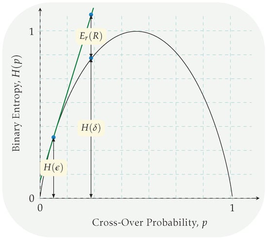
Methodology for establishing the feasible region of β Observe that, since the parameter β adjusts the radius of the hyper spheres used in the codebook construction, a trivial restriction on it would be as follows: . Next, employing the Hamming distance property of Lemma 1 and Lemma 2, β can not be greater or equal than 1; therefore, we conclude that . Now, we exclude the boundary points , since it makes the upper bounds on the κ equal to zero (), which is a contradiction since . Next, we focus on the arguments of and given in (A58) and (A59); see Figure 7. First, observe that the function (cf. (17)) has no zero, and is monotonically increasing for . Second, note that the function (cf. (17)) is decreasing for with a zero at ; therefore, the subsequent feasible interval for β is yielded:
Figure 7.
Depiction of the error exponent for a BSC. The tangent line of the binary entropy function in the cross-over probability point , calculated for , marked in green, is denoted by . For a given cross-over probability , the difference between and is referred to as the error exponent. For example, the upper bounds on the goal identification rate calculated in (A58) and (A59) are two different error exponents that are derived in the sort II error analysis. The minimum of these error exponents is the bottleneck for the rate , i.e., an eligible upper bound.
Observe that the function is continuous and monotonically increasing for domain . That is, tends to zero for asymptotic small β and tends to one for arbitrary.
Remark 4.
Trade-off between goal identification rate and attainable DKI/RKI rate Our results in the achievability proof unveil a common behavior between the DKI and RKI problems; namely, for a given codeword length, there is a trade-off between the size of the goal message set and DKI/RKI codebook size. Specifically, considering the RKI problem for a DMC with zero sort I error probability (cf. (A65)), or obtained inner bound on the set of all attainable rate pairs for a DMC (cf. (4)), we deduce that if one allows for larger goal identification coding rate κ, subsequently a penalty on the upper bound for the attainable RKI rate, R, is incurred, and this upper bound would be decreased. A similar observation for the DKI problem as considered in this paper is found, namely, the same trade-off between attainable DKI coding rate R and goal identification rate κ exist. In particular, the calculated upper bounds provided in (16) on R and κ suggest that for asymptotic small , while the upper bound on κ tends to zero ( for ), the upper bound on R is increased. On the other hand, in one allows that arbitrary, then upper bounds on κ and R are increased and decreased, respectively.
Remark 5.
In the analysis for the sort II error probability, an upper bound is found which vanishes exponentially in the codeword length n, (cf. (A51)). This observation reveals that the fastest scales for the size of the goal message set , which guarantees the vanishing of the sort II error probability, as is permitted to be defined as follows: . In other words, the upper bound on the sort II error probability is capable of being exploited for having a set of goal messages with exponential size.
4.3. Upper Bound (Converse Proof)
Before we start the converse proof, some comprehensive steps are explained: We show that the feasible input set (subset of the input sequences that fulfills the Hamming constraint) can be entirely exhausted for selection of the codewords. To this end, we establish an one-to-one mapping between the message and input sets. Hence, the number of messages is bounded by the size of the feasible input set. More specifically, depending on whether or not an effective Hamming weight constraint is imposed on the input of the channel, we divide it into two cases and address them separately. In particular, the converse proof for each case consists of the subsequent two main technical steps.
- ◊
- Step 1: we show in Lemma 3 that for any attainable DKI rate whose error probabilities of sort I and sort II tends to zero as , any pair of distinct messages are associated with different codewords.
- ◊
- Step 2: exploiting Lemma 3, we acquire an upper bound for the DKI codebook size of a the BSC.
We begin with the below lemma on a DKI codebook size.
Lemma 3
(DKI codebook size). Consider a sequence of -BSC-DKI codes , such that and tend to zero as . Then, given a sufficiently large n, the codebook satisfies the subsequent property: two different messages cannot have the same codeword representing them; that is,
Proof.
Contrarily, suppose that there are two messages and , such that , and
for some . Since forms a -BSC-DKI code, as stated in Definition 1, it implies that for every possible choice (arrangement) of the goal message set of size K, the upper bound on the sort I and sort II error probabilities, i.e., and , respectively, tends to zero as n tends to infinity.
Remark 6.
Decoder in converse proof While we imposed a concrete structure on the decoding set , in the achievability proof provided in Section 4.2, i.e., we set , the converse proof treats the decoding set as a generic function.
Next, we review the definition of a BSC DKI code found in (1), and concentrate on the underlying presumptions about the characteristics of a particular series of BSC DKI codes found in Lemma 3. The subsequent property is endowed by such a code sequence with five parameters, . For any overall/generic selection of the goal message, set of size K, as n approaches to infinity, the upper bound on the sort I and sort II error probabilities, or and , respectively, tends to zero. That is,
Next, we will represent a particular class of the goal message sets by , where and , i.e.,
Observe that ; that is, there exists at least one arrangement belonging to , where . This is valid as the two messages and are different, i.e., , in accordance with Lemma 3. The sort I and sort II error probability, so have the subsequent upper bounds:
where is the decoding set considered for the set of goal messages . This leads to a contradiction, since
where the last inequality exploits the definition of sort I/II error probabilities given in (8) and (9). Therefore, , which is a contradiction to (60).
Put differently, Lemma 3 asserts that every given sequence of BSC DKI codes has the below property: The upper limits on the sort I and sort II error probabilities disappear for an arbitrary (generic) choice of of size , meaning that and tend to zero as . Nevertheless, we demonstrate that there are specific options for , shown by , whose elements does not satisfy this property, namely, and do not disappear since the sum of the corresponding upper limits on the sort I and sort II errors is lower bounded by one. This observation is obviously contradictory, as the inequality presented in (59) does not hold. Hence, distinct messages and cannot share the same codeword, and there exist an one-to-one mapping between the message set and the codebook . This concludes the proof of Lemma 3. □

Lemma 3 states that every message has a distinct/unique codeword. As a result, the number of input sequences that meet the input restriction/constraint serves as the maximum number of messages. We divide in two cases, namely, where and . For the first case, we obtain the subsequent upper bound on the size of the DKI codebook:
where exploits the upper bound on the volume of the Hamming ball provided in Lemma A2 for . Thereby, (64) implies
On the other hand, for a given sequence of DKI code in the converse, the size of the goal message set is always upper bounded by the size of the message set ; that is, gives . Therefore, exploiting (65), we obtain
Now, we proceed to calculate the upper bound on the size of the DKI codebook, where . We argue that this case is equivalent to having a Hamming weight constraint of the form . That is, the codewords with constraint , where fulfilled the same constraint with . The new Bernoulli input process has success probability, i.e., . Therefore, again employing Lemma A2 for the critical point , we obtain
which implies

In this instance, the size of the complete input set, i.e., , that is, the number of input sequences, is a maximum amount on the number of messages. Therefore, we can establish the subsequent upper bound on the size of the DKI codebook which, for , implies
Next, similar to the provided arguments for deriving (66), we obtain
Observe that the established upper bound on the DKI coding rate R as provided in (65), (68) and (69) and implies that the set of all attainable rate pairs is contained as follows:
where
where and are provided in (A58) and (A59), respectively.
Thus, exploiting the fact that DKI capacity region is the closure of the set of all attainable rate pairs is contained as follows:
Thereby, the relations provided in (56) and (71) complete the proof of Theorem 1.
5. Future Directions and Summary
In this work, the deterministic K-identification problem for IoT systems was studied. The results obtained in this paper can serve as a model for tasks that are based on an event recognition within the context of future IoT applications. Specifically, we consider IoT systems that can be modeled by the binary symmetric channel. For this setup, we established inner and outer bounds on the DKI capacity region with/without the Hamming weight constraint for a codebook size of . Our results in this work regarding the DKI capacity for the BSC model unveiled that the conventional exponential scale of considered for the DI [32] and TR problems [17], is the appropriate scale for the codebook size of the DKI problem of the BSC with/without Hamming weight constraint. This observation is was proved by finding a suitable ball covering for an n-dimensional Hamming hyper ball or the entire input set in the same line of arguments as that for the basic Gilbert bound method. In particular, in the presence of a Hamming weight constraint A, we pack hyper balls with radius , for some inside a larger Hamming hyper ball, which results in ∼ codewords. We remind you that the scale of the codebook for DKI over the BSC is lower than that for the DKI over slow fading channels [51] or the DI over Poisson channel with and without ISI [48,52]. Moreover, we find out that the BSC features an exponentially large set of the goal messages set, in the codeword length, n, i.e., ; and characterize the entire feasible range on the goal identification rate as a function of the channels statistic and the Hamming constraint (for ).
For the converse part, a similar approach as our previous work for DI over the DMC [32] is followed. That is, for the case where a non-trivial Hamming weight constraint is present (), we establish an one-to-one mapping between the message set and the feasible set induced by the Hamming weight constraint. In particular, we exploit the method of proof by the contradiction. Namely, we first assume that two generic different messages and share the common codewords, and then show that such an assumption leads to a contradiction regarding the sum of the error probabilities, i.e., we derive that the sum of the sort I and sort II error probabilities converges to one. Hence, the falsehood of the early assumption is guaranteed, and the total number of messages is bounded by the size of the feasible input set, i.e., . For the case where , (absent of a Hamming constraint), a similar line of argument can be applied in order to establish the one-to-one function.
There are numerous ways to expand upon the findings we have showcased in this manuscript. Some of the possible topics for the future research are as follows:
- ◊
- Explicit code construction: In this paper, we mainly address the determination of basic performance constraints for the DKI for the BSC with/without Hamming weight constraint, where an explicit code construction was not investigated. That is, in the achievability proof, we only guarantee the existence of a code without suggesting a systematic method for construction of the code. Therefore, an important direction for research may be explicit construction of K-identification codes for the BSC and development of efficient encoding and low complexity decoding schemes. Furthermore, the efficiency of such concrete designs can be measured versus the information theoretical bounds derived in this paper.
- ◊
- Generalized channel models: We consider in this work one of the simplest and most basic channel model, namely the BSC in the absence of channel state, memory, or feedback. Therefore, our result can be extended to a DMC (with or without memory/feedback), compound, and arbitrary varying channels, which are generalizations of the BSC. In particular, several realistic IoT scenarios modeled by the BSC feature memory to some extent and the effect of memory may not be made negligible in a straightforward manner. Therefore, the application of memoryless channels as conducted in this paper to these realistic instances may in general yields different capacity results. In addition, it may be possible to exploit the memory effect in terms of gaining more optimum inner and outer bounds on the DKI capacity, as well as the specification of the encoding and decoding modules; cf. [61,67,68,69] for detailed studies on the BSC models with memory.
- ◊
- Multi-user and multi-antenna systems: The results in this paper study a point-to-point single user system, and might be extended to advanced scenarios proper for the future communication network settings including multiple-input multiple-output channels or multi-user channels, which are deemed to be more relevant in the complex IoT systems.
- ◊
- Finite codeword length coding: The obtained bounds on the K-identification capacity region studied in this paper determine the performance limits of BSC with/without Hamming weight constraint when the codeword length can grow arbitrarily. However, in practical applications, the codeword length is finite, where there is no way to afford significant encoding/decoding delays. As a result, studying the non-asymptotic DKI capacity of the BSC is an interesting direction for future research.
Author Contributions
Conceptualization, M.J.S. and O.D.; methodology, M.J.S.; validation, C.D. and H.B.; formal analysis, M.J.S. and O.D.; resources, C.D. and H.B.; writing—original draft preparation, M.J.S.; writing—review and editing, M.J.S., O.D., C.D. and H.B.; visualization, M.J.S. and O.D.; supervision, H.B.; project administration, H.B.; funding acquisition, C.D. and H.B. All authors have read and agreed to the published version of the manuscript.
Funding
This research was funded by the German Federal Ministry of Education and Research (BMBF) within the 6G-life project grant number 16KISK002 (M.J.S.), the German Research Foundation (DFG) within the Gottfried Wilhelm Leibniz Prize grant number BO 1734/20-1 (H.B.), the BMBF within the national initiative for “Post-Shannon Communication (NewCom)” with the project “Basics, Simulation and Demonstration For New Communication Models” grant number 16KIS1003K (H.B.), the BMBF within the national initiative for “Post-Shannon Communication (NewCom)” with the project “Coding Theory and Coding Methods For New Communication Models” grant number 16KIS1005 (C.D.), the DFG within Germany’s Excellence Strategy grant number EXC-2111—390814868 and EXC-2092 CASA—390781972 (H.B.), the BMBF grant number 16KIS1005 (C.D.) and the DFG Project grant number DE1915/2-1 (C.D.), the BMBF in the program of “Souverän. Digital. Vernetzt.”, joint project 6G-life, project identification grant number 16KISK002.
Data Availability Statement
The data presented in this study are available in this article.
Conflicts of Interest
The authors declare no conflicts of interest.
Abbreviations
The subsequent abbreviations are used in this manuscript:
| IoT | Internet of Things |
| IoMT | Internet of Medical Things |
| pH | Potential Hydrogen |
| IoBNT | Internet of Bio-Nano Things |
| MC | Molecular Communications |
| 6G | Sixth-Generation |
| PSC | Post-Shannon Communications |
| XG | Future-Generation |
| BSC | Binary Symmetric Channel |
| TR | Shannon’s Message Transmission |
| Bern | Bernoulli |
| DI | Deterministic Identification |
| DMC | Discrete Memoryless Channel |
| RV | Random Variable |
| Vol | Volume |
| DKI | Deterministic K-Identification |
| CDF | Cumulative Distribution Function |
| RI | Randomized Identification |
| RKI | Randomized K-Identification |
| DTPC | Memoryless Discrete-Time Poisson Channel |
| GSF | Gaussian Channel With Slow Fading |
| GV | Gilbert–Varshamov |
| ISI | Inter-Symbol Interference |
| CRF | Channel Reliability Function |
Appendix A. Sort I Error Analysis
Consider the sort I error, i.e., the transmitter sends , yet for every . The sort I error probability is given by
where follows by De Morgan’s law, i.e., and holds since . Now, observe that
where follows by (52) and holds by (12). In order to bound (A2), we proceed to apply the bound provided in (A86) given in Lemma A4: Observe that
where follows, since for real x and holds by (50). On the other hand,
where follows by (50) and holds since is upper bounded by the boundary value of , i.e., where . Observe that the last inequality in (A4) holds for sufficiently large n. Now, since the inequalities provided in (A3) and (A4) fulfill the conditions in Lemma A4, we employ Lemma A4 to establish the following lower bound on (A2) as follows
Observe that the denominator in (A5) is always a strict positive term, since assuming we arrive to a trivial inequality as follows
which is already verified in (A3). Now, we proceed to find a simplified upper bound on the left hand side coefficient in the bracket given in (A5) as follows:
where holds by exploiting for real x and simplifying the denominator by distributing over the bracket, and follows, since
where the first inequality follows since for real x. Thereby, employing (A10) unto (A5), we obtain
Observe that the exponent of exponential term is always strictly positive, since for , the arguments of and are strictly less than . That is, we have the following
The argument is as follows:
which is strictly less than in the asymptotic, i.e., as , where and follows by the same arguments given for (A4), and follows since for real x.
Therefore, the difference for the evaluation of and for a given fix argument is always a strict positive value; see Figure 7. Hence, holds for sufficiently large n and arbitrarily small . Thereby, the sort I error probability satisfies . This complete the analysis for the sort I error probability.
Appendix B. Sort II Error Analysis
In the following, we address sort II errors, i.e., when while the transmitter sent with . Then, for each possible cases of , where , the sort II error probability is given by
where follows by (51), holds by (52) and follows by the union bound, i.e., the sum of each individual event’s probability sets an upper constraint on the probability of the union of events. Let us define the following events
Next, employing the law of total probability with respect to the event , we establish an upper bound on given in (A15) as follows:
where holds by the law of total probability, follows since , holds by (A16), and exploits (A12).
Now, we focus on the event . Let
where follows by the assumption made in the code construction regarding the minimum Hamming distance; see Lemma 1 and (42). Now, without loss of generality, we may assume that the two sequence and differ in the first d symbols, i.e.,
where y is the realization of vector . Therefore, the last symbols (bits) of and are identical. Observe that the event implies that the received vector y and differ in p bits, where , i.e.,
Now, we assume that bits out of the p bits happen in the first d bits, i.e., , where
and bits with happens in last bits, i.e., , where
Observe that since the symbols of sequences are bits, i.e., either 0 or 1; therefore, implies that the two sequences and are complementary for the first d bits. Now, we infer that if the two sequences and differ in , then and are identical in those bits. Hence, .
Now, if we collect all the positions for which and differ, we obtain
Observe that, since we restrict ourselves to the event
On the other hand, since , we obtain
Now, in order to calculate in (A15), we first fix , and then sum up over all possible cases for the , then we would have a second sum which runs for values of from 0 to d. Observe that the has two upper bounds given in (A26) and (A27); therefore, in the calculation, we restrict ourselves to the minimum of those two upper bounds. Let define . Thereby,
where holds since , and follows since every expression that is independent of the sum’s variable can be shifted left behind the inner sum. In , we have added , to obtain the correct form for the two binomial distribution expressions. Now, observe that the first sum is the Binomial cumulative distribution function at point and can be upper bounded by 1, i.e.,
Now, let focus on the second sum in (A28), for which we establish an upper bound by maximizing through setting , i.e.,
Therefore,
where the last equality holds since by for real , we obtain .
Now, we exploit the inequality (A95) given in Lemma A5 to obtain an upper bound for the second sum in (A28) as follows: First, we check whether the required condition in Lemma A5 are satisfied or not. Namely, we set and . Now, we calculate their ratio as follows:
where holds since for real x and holds by the following argument: we assume that holds and assuming that , we arrive at a trivial inequality, namely,
which can be deduced by assumptions of code construction given in (42), i.e.,
where holds, since for real . Now, we exploit (50), to show that (A32) is upper bounded by as follows
Thereby, we apply safely Lemma A5 with parameters , and , and obtain
Let us focus on the coefficient in (A41). In the following, assuming an upper bound for it, we arrive to a trivial inequality, therefore, the upper bound is valid.
Observe that (A42) yield the following chain of expressions:
which is trivial, since it is already proved in (A32). Now, observe that for , the following holds
see Figure 7. Therefore, since always yield a smaller exponent, we obtain an upper bound on the sum in (A41) as follows
where exploits (A42), and follows by (A48). Thereby, recalling (A28) and employing (A29), we obtain
Hence, recalling (A15) and (A18), we obtain
which implies that both the exponential factors given in (A51) should yields strict positive exponents; that is, we obtain two separate upper bounds on the as follows:
Therefore,
Now, we focus on the second argument in (A53), and provide the following asymptotic behavior:
where the equality holds, since and are continuous functions of . Now, observe that since for real , we obtain
where holds by the squeeze theorem. Thereby,
Thus, recalling (A53), we obtain the subsequent upper bound on the goal identification rate :
where follows from (A32) and (A56). Next, exploiting (49), we derive the arguments provided in (A57) as follows:
where and are given in (13) and (14). Thereby,
Therefore, recalling (A51), we obtain
hence, holds for sufficiently large n and arbitrarily small .
Appendix C. Cover-Free Families
In this subsection, we provide some preliminaries about the concept of cover-free families and establish some basic and well-known results. Furthermore, we draw the connection between such concept and the RKI.
Definition A1
(r-cover-free family). Let pair be a set system, where X is a set of points and is a set of subsets (blocks) of X. A set system is called r-cover-free family, if for an arbitrary r distinct blocks and any other block , we have
The concept of r-cover-free families in the literature was first found in [70]. In the following, we introduce a well-known theorem in the literature, which established a power law decaying the lower and upper bounds on the size of cover-free families.
Theorem A1
(see [70]). Let and be the set of points and subsets, respectively, such that the set system constitute a r-cover-free family. Then, let indicate the maximum size of over 𝒜 by . Now, we have
for some constants and .
Next, we present a theorem which establish an upper bound on the size of r-cover-free family as follows:
Theorem A2
(see [71]). Assume that set system constitute a r-cover-free family where . Now, the maximum size of the r-cover-free family, i.e., , is upper bounded as follows:
where k is a constant.
Next, we explain on the connection between the notion of r-cover-free families in the combinatorics and RKI for noiseless discrete memoryless channel found by Ahlswede in [26]: Let , , , then the RI coding with 0-valued first type error, is upper bounded by:
Then, for a DMC with input alphabet of size , we obtain
Therefore, for the binary input channel, i.e., where , we obtain .
Appendix D. Lower Bound on the Volume of the Hamming Ball
Lemma A1
(see [72], Lem. 16.19). Let be positive integers and assume a real ε where . Then, volume of the Hamming ball in the q-ary alphabet is lower bounded as follows:
Proof.
Observe that the Stirling approximation [73] gives the following bounds on :
Now, we have
where holds, since we let
and holds, since
Next, we proceed to bound the Hamming ball as follows: Observe that the volume of Hamming ball as provided in (A66) is lower bounded by the Binomial coefficient for the largest index, i.e., . Therefore,
Now, by letting and , we obtain
where follows for sufficiently large n, since and holds by setting . Therefore,
which implies that
Thereby,
□
Appendix E. Upper Bound on the Volume of the Hamming Ball
Lemma A2
(see [72], Lem. 16.19). Let integer and with . Then, volume of the Hamming ball in the binary alphabet is upper bounded as follows:
Proof.
Note that , the logit function is non-positive, i.e.,
Next, notice that for we obtain the following:
where is the binary entropy function. Hence, . Now,
□
Therefore, we obtain
Appendix F. Bound on the Upper Tail of the Binomial Cumulative Distribution Function—Part 1
Lemma A3
(see ([35 Probl. 5.8-(c))). Let and . Then,
Proof.
The proof for the lower bound is trivial and obvious. For proving the upper bound, we employ the provided hints given in ([35] p. 531) as follows: Observe that
and
Using the induction, we obtain
Now, we sum over the variable j by using a geometric series. Next, we combine this results with the result of part in the Problem 5.8 of [35], and we obtain the desired upper bound. That is,
□
Appendix G. Bound on the Upper Tail of the Binomial Cumulative Distribution Function—Part 2
Lemma A4.
Let and . Then,
Proof.
Recall that the equation of the tangent line to the binary entropy function at the specific point is given by
where holds by definition of a tangent line to a function at specific point, follows since derivative of the entropy function reads the negative of the logit function, i.e.,
for , and holds by definition of the entropy function, i.e.,
Therefore, exploiting (A87) we obtain,
which implies . Thereby,
Now, observe that the Binomial coefficient where and , can be upper bounded as follows ([34] see p. 353)
Therefore,
where holds by (A91), and follows by exploiting (A91). Now, recalling (A86), we obtain
This completes the proof of Lemma A4. □
Appendix H. Bound on the Binomial Cumulative Distribution Function
Lemma A5
(see ([74] App. A)). Let and with . Then,
Proof.
Let us define
i.e., and or equivalently
Now, observe that .
Furthermore, by definition of the binary entropy function and its tangent line, we have
and
where (A98) follows by (A89) and (A99) holds by (A90).
Now, applying the variable exchange of unto (A86), we obtain
Observe that, since the index of sum in (A86) runs form k to n, i.e., , in the new system, we have , which is equivalent to . Further, the Binomial coefficient for fulfills the subsequent identity:
Thereby,
Now, applying the exchange of variables given in (A97) unto (A102), we obtain
where the equality holds by (A98) and (A99). Therefore,
Now, we focus on the bracket in (A103), which can be simplified as follows:
where the first equality follows by dividing both sides in the left side by factor n. Thereby,
This completes the proof of Lemma A5. □
References
- Li, S.; Xu, L.D.; Zhao, S. The Internet of Things: A Survey. Inf. Syst. Front. 2015, 17, 243–259. [Google Scholar] [CrossRef]
- Da Xu, L.; He, W.; Li, S. Internet of Things in Industries: A Survey. IEEE Trans. Ind. Inform. 2014, 10, 2233–2243. [Google Scholar]
- Stankovic, J.A. Research Directions For The Internet of Things. IEEE Internet Things J. 2014, 1, 3–9. [Google Scholar] [CrossRef]
- Sun, L.; Du, Q. A Review of Physical Layer Security Techniques For Internet of Things: Challenges and Solutions. Entropy 2018, 20, 730. [Google Scholar] [CrossRef] [PubMed]
- Batty, M.; Axhausen, K.W.; Giannotti, F.; Pozdnoukhov, A.; Bazzani, A.; Wachowicz, M.; Ouzounis, G.; Portugali, Y. Smart Cities of The Future. Eur. Phys. J. Spec. Top. 2012, 214, 481–518. [Google Scholar] [CrossRef]
- Ray, P.P. An Introduction to Dew Computing: Definition, Concept and Implications. IEEE Access 2018, 6, 723–737. [Google Scholar] [CrossRef]
- Jordan, M.I.; Mitchell, T.M. Machine Learning: Trends, Perspectives, and Prospects. Science 2015, 349, 255–260. [Google Scholar] [CrossRef]
- Paiva, S.; Ahad, M.A.; Tripathi, G.; Feroz, N.; Casalino, G. Enabling Technologies For Urban Smart Mobility: Recent Trends, Opportunities and Challenges. Sensors 2021, 21, 2143. [Google Scholar] [CrossRef]
- Mahmud, K.; Town, G.E.; Morsalin, S.; Hossain, M. Integration of Electric Vehicles and Management in The Internet of Energy. Renew. Sustain. Energy Rev. 2018, 82, 4179–4203. [Google Scholar] [CrossRef]
- Fascista, A.; Coluccia, A.; Ravazzi, C. A Unified Bayesian Framework For Joint Estimation and Anomaly Detection in Environmental Sensor Networks. IEEE Access 2023, 11, 227–248. [Google Scholar] [CrossRef]
- Gatouillat, A.; Badr, Y.; Massot, B.; Sejdić, E. Internet of Medical Things: A Review of Recent Contributions Dealing With Cyber-Physical Systems in Medicine. IEEE Internet Things J. 2018, 5, 3810–3822. [Google Scholar] [CrossRef]
- da Costa, C.A.; Pasluosta, C.F.; Eskofier, B.; da Silva, D.B.; da Rosa Righi, R. Internet of Health Things: Toward Intelligent Vital Signs Monitoring in Hospital Wards. Med. Artif. Intell. 2018, 89, 61–69. [Google Scholar] [CrossRef]
- Lee, C.; Koo, B.H.; Chae, C.B.; Schober, R. The Internet of Bio-Nano Things in Blood Vessels: System Design and Prototypes. J. Commun. Netw. 2023, 25, 222–231. [Google Scholar] [CrossRef]
- Akyildiz, I.F.; Pierobon, M.; Balasubramaniam, S.; Koucheryavy, Y. The Internet of Bio-Nano Things. IEEE Commun. Mag. 2015, 53, 32–40. [Google Scholar] [CrossRef]
- Nakano, T.; Eckford, A.W.; Haraguchi, T. Molecular Communication; Cambridge University Press: New York, NY, USA, 2013. [Google Scholar]
- Farsad, N.; Yilmaz, H.B.; Eckford, A.; Chae, C.B.; Guo, W. A Comprehensive Survey of Recent Advancements in Molecular Communication. IEEE Commun. Surv. Tutor. 2016, 18, 1887–1919. [Google Scholar] [CrossRef]
- Shannon, C.E. A Mathematical Theory of Communication. Bell Syst. Tech. J. 1948, 27, 379–423. [Google Scholar] [CrossRef]
- Cabrera, J.A.; Boche, H.; Deppe, C.; Schaefer, R.F.; Scheunert, C.; Fitzek, F.H. 6G and the Post-Shannon Theory. In Shaping Future 6G Networks: Needs, Impacts, and Technologies; IEEE Press: Piscataway, NJ, USA, 2021; pp. 271–294. [Google Scholar]
- Zhang, C.; Zou, H.; Lasaulce, S.; Saad, W.; Kountouris, M.; Bennis, M. Goal-Oriented Communications For The IoT and Application to Data Compression. IEEE Internet Things Mag. 2022, 5, 58–63. [Google Scholar] [CrossRef]
- Schwenteck, P.; Nguyen, G.T.; Boche, H.; Kellerer, W.; Fitzek, F.H.P. 6G Perspective of Mobile Network Operators, Manufacturers, and Verticals. IEEE Netw. Lett. 2023, 5, 169–172. [Google Scholar] [CrossRef]
- Fettweis, G.P.; Boche, H. 6G: The Personal Tactile Internet—And Open Questions for Information Theory. IEEE BITS Inf. Theory Mag. 2021, 1, 71–82. [Google Scholar] [CrossRef]
- Liu, Y.; Liu, X.; Mu, X.; Hou, T.; Xu, J.; Di Renzo, M.; Al-Dhahir, N. Reconfigurable Intelligent Surfaces: Principles and Opportunities. IEEE Commun. Surv. Tutor. 2021, 23, 1546–1577. [Google Scholar] [CrossRef]
- Fascista, A.; Keskin, M.F.; Coluccia, A.; Wymeersch, H.; Seco-Granados, G. RIS-Aided Joint Localization and Synchronization With a Single-Antenna Receiver: Beamforming Design and Low-Complexity Estimation. IEEE J. Sel. Top. Signal Process. 2022, 16, 1141–1156. [Google Scholar] [CrossRef]
- Shi, J.; Chan, T.T.; Pan, H.; Lok, T.M. Reconfigurable Intelligent Surface Assisted Semantic Communication Systems. arXiv 2023, arXiv:2306.09650. [Google Scholar]
- Torres-Figueroa, L.; Ferrara, R.; Deppe, C.; Boche, H. Message Identification for Task-Oriented Communications: Exploiting an Exponential Increase in the Number of Connected Devices. IEEE Internet Things Mag. 2023, 6, 42–47. [Google Scholar] [CrossRef]
- Ahlswede, R. General Theory of Information Transfer: Updated. Discrete Appl. Math. 2008, 156, 1348–1388. [Google Scholar] [CrossRef]
- Seyhan, K.; Akleylek, S. Classification of Random Number Generator Applications in IoT: A Comprehensive Taxonomy. J. Inf. Secur. Appl. 2022, 71, 103365. [Google Scholar] [CrossRef]
- Hughes, J.P.; Diffie, W. The Challenges of IoT, TLS, and Random Number Generators in The Real World: Bad Random Numbers are Still With us and Are Proliferating in Modern Systems. Queue 2022, 20, 18–40. [Google Scholar] [CrossRef]
- Brakerski, Z.; Kalai, Y.T.; Saxena, R.R. Deterministic and Efficient Interactive Coding From Hard-to-Decode Tree Codes. In Proceedings of the IEEE Symposium on Foundations of Computer Science, Durham, NC, USA, 16–19 November 2020; pp. 446–457. [Google Scholar]
- Bocchino, R.L.; Adve, V.; Adve, S.; Snir, M. Parallel Programming Must be Deterministic by Default. Usenix HotPar 2009, 6, 1855591–1855595. [Google Scholar]
- Arıkan, E. Channel Polarization: A Method For Constructing Capacity-Achieving Codes For Symmetric Binary-Input Memoryless Channels. IEEE Trans. Inf. Theory 2009, 55, 3051–3073. [Google Scholar] [CrossRef]
- Salariseddigh, M.J.; Pereg, U.; Boche, H.; Deppe, C. Deterministic Identification Over Channels With Power Constraints. IEEE Trans. Inf. Theory 2022, 68, 1–24. [Google Scholar] [CrossRef]
- JáJá, J. Identification is Easier Than Decoding. In Proceedings of the Annual Symposium on Foundations of Computer Science, Portland, OR, USA, 21–23 October 1985; pp. 43–50. [Google Scholar]
- Cover, T.; Thomas, J. Elements of Information Theory; Wiley Series Telecomm.; John Wiley & Sons: New York, NY, USA, 1991. [Google Scholar]
- Gallager, R.G. Information Theory and Reliable Communication; John Wiley & Sons, Inc.: New York, NY, USA, 1968. [Google Scholar]
- Gamal, A.E.; Kim, Y.H. Network Information Theory; Cambridge University Press: New York, NY, USA, 2012. [Google Scholar]
- MacKay, D.J. Information Theory, Inference and Learning Algorithms; Cambridge University Press: New York, NY, USA, 2003. [Google Scholar]
- Zhang, G.; Chen, K.; Ma, C.; Reddy, S.K.; Ji, B.; Li, Y.; Han, C.; Zhang, X.; Fu, Z. Decision Fusion For Multi-Route and Multi-Hop Wireless Sensor Networks Over The Binary Symmetric Channel. Comput. Commun. 2022, 196, 167–183. [Google Scholar] [CrossRef]
- Premkumar, K.; Chen, X.; Leith, D.J. Utility Optimal Coding For Packet Transmission Over Wireless Networks—Part I: Networks of Binary Symmetric Channels. In Proceedings of the 49th Annual Allerton Conference on Communication, Control, and Computing (Allerton), Monticello, IL, USA, 28–30 September 2011; pp. 1592–1599. [Google Scholar] [CrossRef]
- Slepian, D. A Class of Binary Signaling Alphabets. Bell Syst. Tech. J. 1956, 35, 203–234. [Google Scholar] [CrossRef]
- Elias, P. Coding For Noisy Channels. In Proceedings of the IRE WESCON Convention Record; 1955; Volume 2, pp. 94–104. Available online: https://cir.nii.ac.jp/crid/1570009750462156928 (accessed on 13 February 2024).
- Elias, P. Coding For Two Noisy Channels. In Proceedings of the 3rd London Symposium in Information Theory, London, UK, September 1955; Available online: https://cir.nii.ac.jp/crid/1571417125336937088 (accessed on 13 February 2024).
- Elias, P. List Decoding For Noisy Channels. In Proceedings of the IRE WESCON Convention Record, San Francisco, CA, USA, 20–23 August 1957; pp. 94–104. [Google Scholar]
- Golay, M.J. Notes on Digital Coding. Proc. IEEE 1949, 37, 657. [Google Scholar]
- Hamming, R.W. Error Detecting and Error Correcting Codes. Bell Syst. Tech. J. 1950, 29, 147–160. [Google Scholar] [CrossRef]
- Reed, I.S. A Class of Multiple-Error-Correcting Codes and The Decoding Scheme. IEEE Trans. Inf. Theory 1954, 4, 38–49. [Google Scholar] [CrossRef]
- Dabbabi, O.; Salariseddigh, M.J.; Deppe, C.; Boche, H. Deterministic K-Identification For Binary Symmetric Channel. arXiv 2023, arXiv:2305.04260. [Google Scholar]
- Salariseddigh, M.J.; Jamali, V.; Pereg, U.; Boche, H.; Deppe, C.; Schober, R. Deterministic Identification For Molecular Communications Over The Poisson Channel. IEEE Trans. Mol. Biol. Multi-Scale Commun. 2023, 9, 408–424. [Google Scholar] [CrossRef]
- Ahlswede, R.; Dueck, G. Identification Via Channels. IEEE Trans. Inf. Theory 1989, 35, 15–29. [Google Scholar] [CrossRef]
- Kumar, S.; Marescaux, J. Telesurgery; Springer Science & Business Media: New York, NY, USA, 2008. [Google Scholar]
- Spahovic, M.; Salariseddigh, M.J.; Deppe, C. Deterministic K-Identification For Slow Fading Channels. In Proceedings of the IEEE Information Theory Workshop (ITW), Saint-Malo, France, 23–28 April 2023; pp. 353–358. [Google Scholar] [CrossRef]
- Salariseddigh, M.J.; Jamali, V.; Pereg, U.; Boche, H.; Deppe, C.; Schober, R. Deterministic K-Identification For MC Poisson Channel With Inter-Symbol Interference. IEEE Open J. Commun. Soc. 2024. [Google Scholar] [CrossRef]
- Abu-Mostafa, Y.S. Complexity in Information Theory; Springer: New York, NY, USA, 1988. [Google Scholar]
- Yao, A.C. Some Complexity Questions Related to Distributive Computing. In Proceedings of the Annual ACM Symposium on the Theory Computing, Atlanta, GA, USA, 30 April–2 May 1979; pp. 209–213. [Google Scholar]
- Verdu, S.; Wei, V. Explicit Construction of Optimal Constant-Weight Codes For Identification Via Channels. IEEE Trans. Inf. Theory 1993, 39, 30–36. [Google Scholar] [CrossRef]
- Günlü, O.; Kliewer, J.; Schaefer, R.F.; Sidorenko, V. Code Constructions and Bounds For Identification Via Channels. IEEE Trans. Commun. 2021, 70, 1486–1496. [Google Scholar] [CrossRef]
- Ahlswede, R.; Cai, N. Identification Without Randomization. IEEE Trans. Inf. Theory 1999, 45, 2636–2642. [Google Scholar] [CrossRef]
- Mehlhorn, K.; Schmidt, E.M. Las Vegas is Better Than Determinism in VLSI and Distributed Computing. In Proceedings of the 14th Annal ACM Symposium on Theory of Computation, San Francisco, CA, USA, 5–7 May 1982; pp. 330–337. [Google Scholar]
- Salariseddigh, M.J.; Jamali, V.; Boche, H.; Deppe, C.; Schober, R. Deterministic Identification For MC Binomial Channel. In Proceedings of the IEEE International Symposium on Information Theory (ISIT), Taipei, Taiwan, 25–30 June 2023; pp. 448–453. [Google Scholar] [CrossRef]
- Yamamoto, H.; Ueda, M. Multiple Object Identification Coding. IEEE Trans. Inf. Theory 2015, 61, 4269–4276. [Google Scholar] [CrossRef]
- Kennedy, R.S. Finite-Sate Binary Symmetric Channels. Ph.D. Thesis, Massachusetts Institute of Technology, Cambridge, MA, USA, 1963. [Google Scholar]
- Rudin, W. Principles of Mathematical Analysis; McGraw-Hill: New York, NY, USA, 1953. [Google Scholar]
- Gilbert, E.N. A Comparison of Signalling Alphabets. Bell Syst. Tech. J. 1952, 31, 504–522. [Google Scholar] [CrossRef]
- Richardson, T.; Urbanke, R. Modern Coding Theory; Cambridge University Press: New York, NY, USA, 2008. [Google Scholar]
- Conway, J.H.; Sloane, N.J.A. Sphere Packings, Lattices and Groups; Springer: New York, NY, USA, 2013. [Google Scholar]
- Van Lint, J.H. Introduction to Coding Theory; Springer Science & Business Media: New York, NY, USA, 1998; Volume 86. [Google Scholar]
- Gilbert, E.N. Capacity of a Burst-Noise Channel. Bell Syst. Tech. J. 1960, 39, 1253–1265. [Google Scholar] [CrossRef]
- Alexander, A.A.; Gryb, R.M.; Nast, D.W. Capabilities of The Telephone Network For Data Transmission. Bell Syst. Tech. J. 1960, 39, 431–476. [Google Scholar] [CrossRef]
- Fontaine, A.B.; Gallager, R.G. Error Statistics and Coding For Binary Transmission Over Telephone Circuits. Proc. IRE 1961, 49, 1059–1065. [Google Scholar] [CrossRef]
- Kautz, W.; Singleton, R. Nonrandom Binary Superimposed Codes. IEEE Trans. Inf. Theory 1964, 10, 363–377. [Google Scholar] [CrossRef]
- Füredi, Z. On r-Cover-Free Families. J. Comb. Theory Ser. A 1996, 73, 172–173. [Google Scholar] [CrossRef]
- Flum, J.; Grohe, M. Parameterized Complexity Theory; Texts in Theoretical Computer Science (An EATCS Series); Springer: New York, NY, USA, 2006. [Google Scholar]
- Robbins, H. A Remark On Stirling’s Formula. Am. Math. Mon. 1955, 62, 26–29. [Google Scholar] [CrossRef]
- Jeřábek, E. Dual Weak Pigeonhole Principle, Boolean Complexity, and Derandomization. Ann. Pure Appl. Log. 2004, 129, 1–37. [Google Scholar] [CrossRef]
Disclaimer/Publisher’s Note: The statements, opinions and data contained in all publications are solely those of the individual author(s) and contributor(s) and not of MDPI and/or the editor(s). MDPI and/or the editor(s) disclaim responsibility for any injury to people or property resulting from any ideas, methods, instructions or products referred to in the content. |
© 2024 by the authors. Licensee MDPI, Basel, Switzerland. This article is an open access article distributed under the terms and conditions of the Creative Commons Attribution (CC BY) license (https://creativecommons.org/licenses/by/4.0/).