Short-Term Mobile Network Traffic Forecasting Using Seasonal ARIMA and Holt-Winters Models

Abstract

Fifth-generation (5G) networks require efficient radio resource management (RRM) which should dynamically adapt to the current network load and user needs. Monitoring and forecasting network performance requirements and metrics helps with this task. One of the parameters that highly influences radio resource management is the profile of user traffic generated by various 5G applications. Forecasting such mobile network profiles helps with numerous RRM tasks such as network slicing and load balancing. In this paper, we analyze a dataset from a mobile network operator in Portugal that contains information about volumes of traffic in download and upload directions in one-hour time slots. We apply two statistical models for forecasting download and upload traffic profiles, namely, seasonal autoregressive integrated moving average (SARIMA) and Holt-Winters models. We demonstrate that both models are suitable for forecasting mobile network traffic. Nevertheless, the SARIMA model is more appropriate for download traffic (e.g., MAPE [mean absolute percentage error] of 11.2% vs. 15% for Holt-Winters), while the Holt-Winters model is better suited for upload traffic (e.g., MAPE of 4.17% vs. 9.9% for SARIMA and Holt-Winters, respectively).

1. Introduction

Fifth-generation (5G) and 6G networks [1,2] are expected to support a wide range of new technologies, such as drones and virtual/augmented reality, which require high bit rates, lower latency, and increased throughput [3,4,5]. The number of connected devices is increasing, resulting in a dramatic growth in traffic volume, causing anomalies such as network congestion, decreased quality of service, network delays, data loss, and blocking of new connections [6]. The network architecture should adapt to the volumes of traffic generated by various applications and use it for decision-making, taking into account several types of traffic with different service and priority requirements [7,8,9]. Artificial intelligence (AI) and machine learning (ML) are now trends for 5G networks that could provide more efficient and reasonable network planning and management [10]. AI and ML models could be trained on a large amount of data that service providers collect [11]. The collected data should be reliable, and the analysis carried out should be accurate [12].

Network traffic forecasting is one of the tasks that use ML methods for effective network management [13,14]. This task aims to identify potential problems before they occur, reduce service outages, manage user needs, and analyze user behavior in applications [15]. For example, traffic forecasting is used for smart power consumption by a base station [11]. In [16], this problem is considered based on network slicing, mobile edge computing, base station sleeping, and additional power during high-demand hours. Traffic forecasting is divided into short-term and long-term, but sometimes medium-term forecasting is also necessary [17].

1.1. Related Work

Forecasting methods typically begin with statistical models, such as ARIMA (autoregressive integrated moving average) [18] and its seasonal variant SARIMA, exponential smoothing (Holt-Winters, extended Holt-Winters, etc.), and regression models (multiple, linear, etc.). In addition, ML and deep learning models, Gaussian models (Gaussian mixture model [19,20], Gaussian process), random forests, and neural networks are also commonly used. While ML models generally outperform statistical models, there are instances where statistical models are applied for their faster processing capabilities. To achieve more accurate results, a combination of different approaches is often utilized [16]. The same applies to network traffic forecasting. LTE (long-term evolution) traffic is predicted by the ARIMA model [21], as well as bagging, random forest, and support vector machines [22]. In [23], the authors used ARIMA for post-processing the residuals of the ML algorithm, which improves the accuracy of traffic prediction. In [24], 5G traffic is forecasted by gated recurrent unit and long short-term memory (LSTM) networks. The authors of [25,26] show that LSTM is good for online forecasting.

Let us review selected papers on the subject of applying statistical models in network traffic forecasting.

Table 1. Summary of selected works on statistical models for network traffic forecasting.

Ref.	Task	Data Source/Application	Model	Evaluation Metric
[30]	Traffic forecasting	Traffic from 2 cells	ARIMA	MAE, NMSE
[31]	Traffic forecasting	Traffic from 3 LTE cells	ARIMA, LSTM	MSE, MAE, $R^2$ score
[34]	Network capacity forecasting	Circuit switch and packet switch 3G traffic	Random walk, Linear trend, Exponential smoothing, ARIMA	RMSE, MAPE
[38]	Traffic forecasting	Traffic from 7160 LTE cells	SARIMA, Holt-Winters, Random Forest, SVM, ANN	MAPE, MAE
[28]	Recourse optimization	Traffic from the network with discontinuous reception (DRX) scheme	ARIMA, LSTM	RMSE
[39]	Traffic congestion forecasting	Traffic from 8 detectors of virtual reality railway	Random walk, Historical mean, ARIMA, LSTM, GRU, DCFCN	RMSE, MAE, MAPE
[36]	Traffic forecasting	Traffic from 470 access points of an enterprise network	Holt-Winters, SARIMA, LSTM, GRU, CNN	MAE, RMSE, NRMSE, $R^2$ score
[40]	Throughput forecasting	Download traffic from HSPA network	ARIMA, FARIMA, ANN	Efficiency, switches per minute and buffering per minute
[35]	Traffic forecasting	WiFi and cellular download traffic from a server	ARIMA, FARIMA, SVR, RNN	MAE, RMSE, MAPE, MASE
[33]	Traffic forecasting	WiFi traffic from 15 protocols	ARIMA	Error rate, average absolute deviation, mean and variance of the error
[41]	Traffic forecasting and anomaly detection	Traffic from wireless sensor network	ARIMA	Complexity, Accuracy, Intelligence, Independence
[32]	Traffic forecasting	Traffic from 191 eNodeB	ARIMA	AIC, AICc, BIC
[42]	Traffic forecasting	WLAN traffic	ARIMA, FARIMA, SVM, Welevet, ANN	MSE, NMSE
[29]	Traffic forecasting	Voice and data traffic from 600 cells	Exponential Smoothing, Holt-Winters	AIC, SSR, RMSE, AMSE
[37]	Spectrum efficiency forecasting	Traffic from 3 countries	AR, MA, ARMA, ARIMA	MAE, MSE, RMSE, NRMSE, NMAE
[43]	Traffic forecasting	Traffic from an institutional wireless network	ARIMA, ANFIS	RMSE
[44]	Traffic forecasting	LTE and 3G traffic	ARIMA	Percentage error between models

provides a summary of these papers in terms of the tasks they address, the applications that generate traffic, the models used, and the metrics used to evaluate these models. Most of the papers focus on traffic forecasting, but the tasks of capacity planning [27] and resource optimization [28] are also addressed. The data are collected from several sources, including cells [29,30,31,32], devices [33], switches [34], and servers [35]. The most commonly used statistical model is the ARIMA model [36,37]. Moreover, combinations of statistical and machine learning methods are used to achieve more accurate results [38,39]. The evaluation metrics help to determine which solutions are most suitable for the proposed model. The choice of metrics depends on the specific study, such as MAE and MSE [30,31], or performance indicators [40].

1.2. Contributions

In this paper, we analyze mobile network traffic collected from a network in Portugal over a half-month period. The available data include the number of megabytes (MB) sent and received by various applications during each hour. Our goal is to forecast the total traffic behavior separately for downlink and uplink using fast processing statistical models.

The main contributions of our study are as follows:

• We analyze the dataset of real network traffic from a mobile operator in Portugal using fast processing statistical models, namely SARIMA, and Holt-Winters, which have not been applied to this data before.
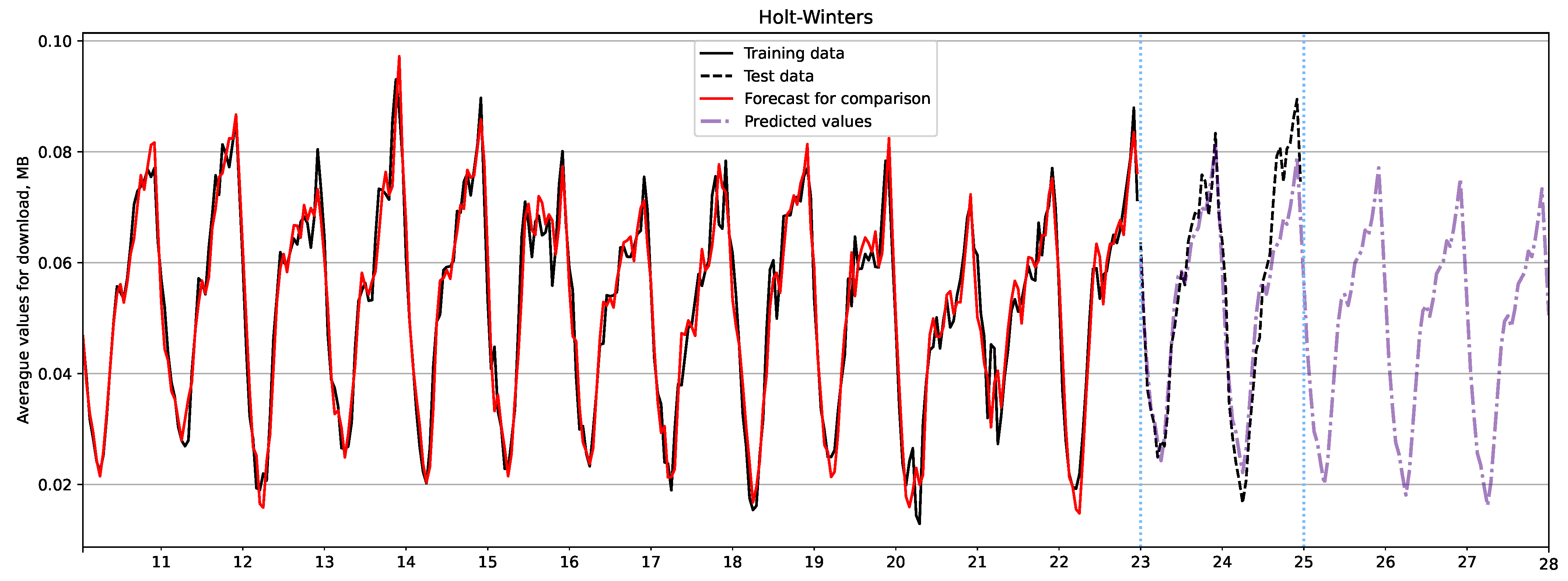
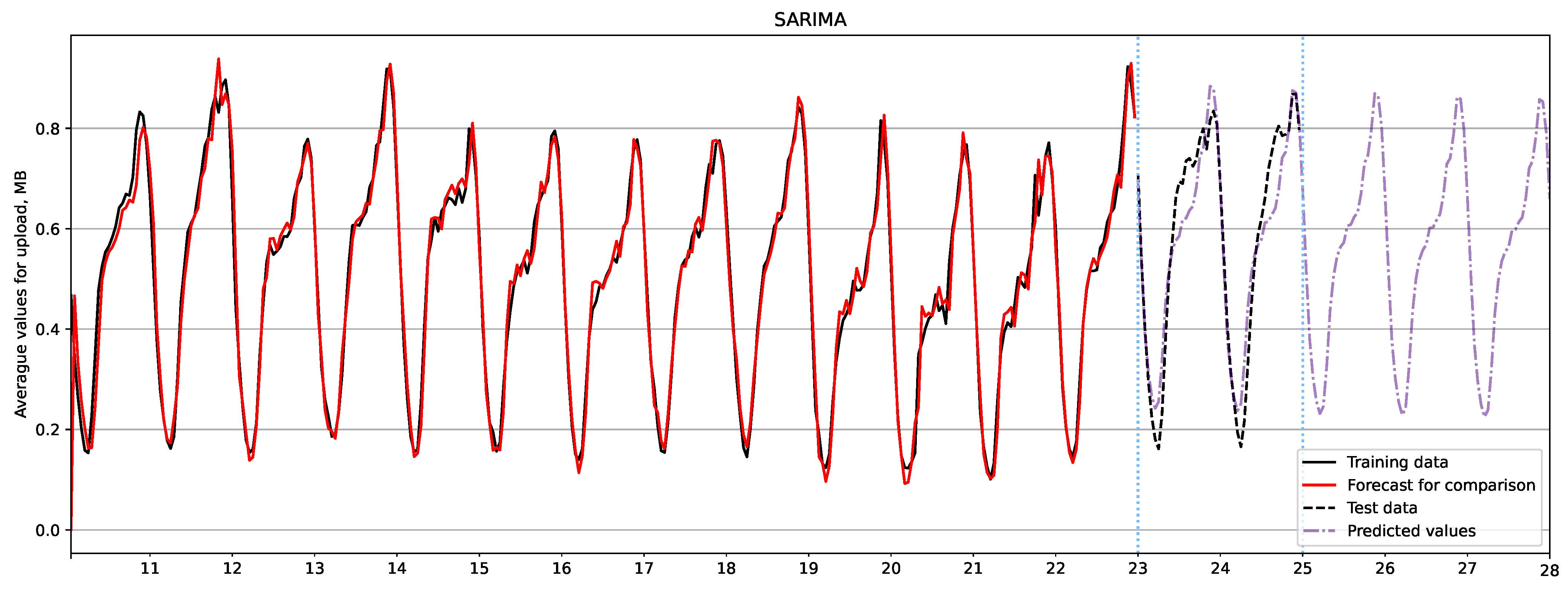
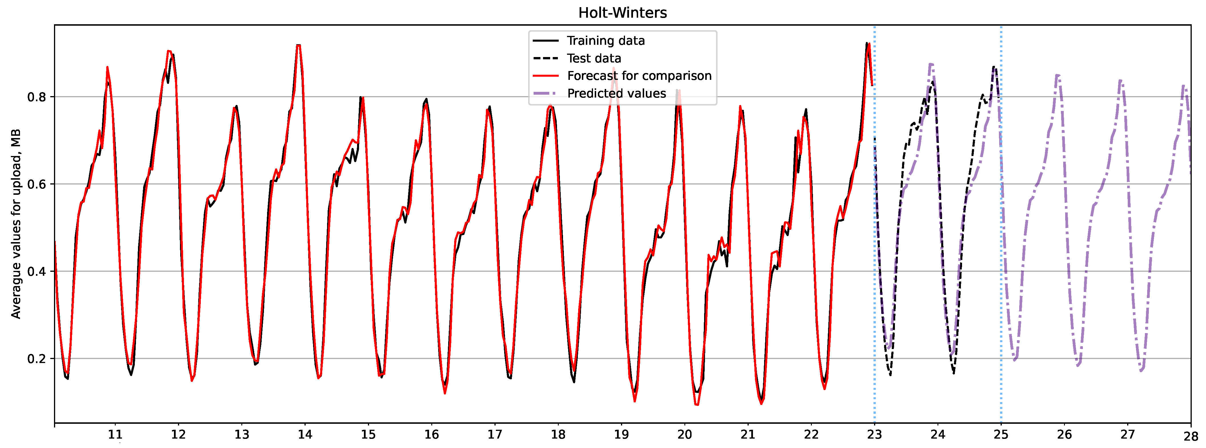
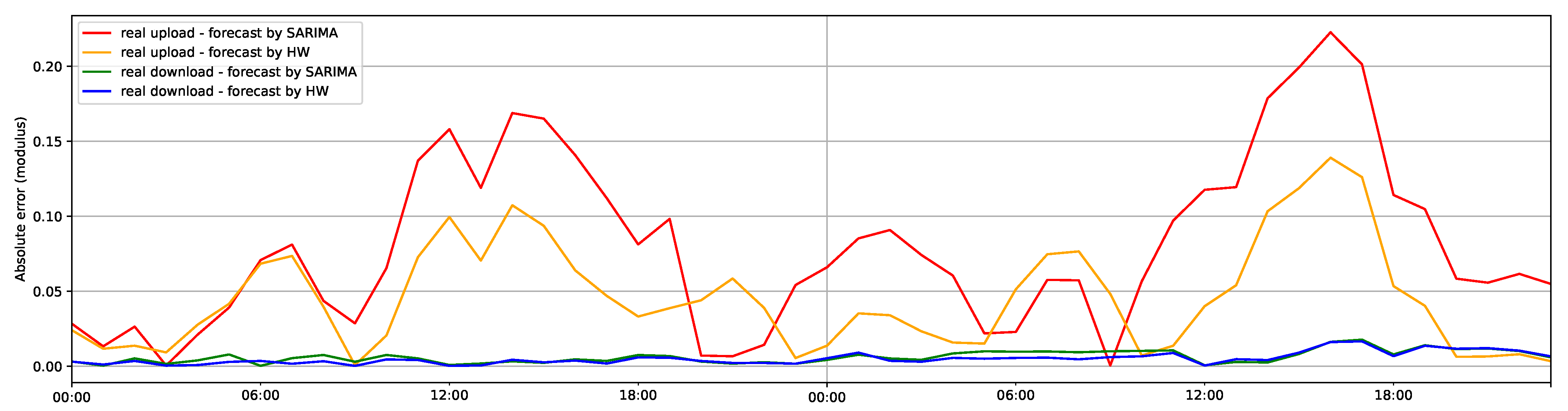
• We demonstrate that the SARIMA model is more appropriate for forecasting download traffic, while the Holt-Winters model is better suited for forecasting upload traffic, showing appropriate errors in the considered dataset.
• Since statistical models are suitable for fast and precise forecasting of mobile network traffic, they can be implemented in cellular operators’ solutions without a significant increase in cost.

The rest of the paper is organized as follows. Section 2 provides a description of the dataset and illustrates the traffic behavior, both in total and by various applications. In Section 3, we discuss the SARIMA and Holt-Winters models, along with the necessary preliminary checks. Section 4 outlines the metrics used for evaluating the models and presents forecasts for both download and upload traffic. Conclusions are drawn in Section 5.

2. Descriptive Statistics

In this section, we will describe the dataset and analyze the overall traffic profile, including the total traffic over all applications and the average traffic for various applications.

2.1. Dataset Description

We use the dataset obtained from a mobile network operator that offers multiple services (applications), such as Internet access, messaging, calls, file transfer, etc. The data flow is bidirectional, with traffic flowing from the base station to the user device in the downlink direction and from the device to the base station in the uplink direction. Each user device is associated with a unique masked mobile station international subscriber directory number (MSISDN). The monitoring system records the upload and download data generated by each device for each application class every hour. The statistics represent the volume of traffic in megabytes (MB) for both the download and upload directions.

Variable descriptions are provided in

Table 2. Dataset variables.

Variable	Description
START_HOUR	Start time of the one-hour period for measuring traffic
MASKED_MSISDN	Masked mobile station international subscriber directory number
APP_CLASS	Application class
UPLOAD	Incoming traffic in the uplink during one hour [MB]
DOWNLOAD	Outgoing traffic in the downlink during one hour [MB]

, and dataset records are presented in

Table 3. Dataset records example.

START_HOUR	MASKED_MSISDN	APP_CLASS	UPLOAD	DOWNLOAD
2018-02-10 01:00:00	F6C1745A0A9DF638DE2C14683E0F250D	Streaming Applications	0.002527	0.000616
2018-02-10 01:00:00	6474B3E3E20B5887A7593C61439250A9	Others	0.000828	0.000334
2018-02-10 01:00:00	B05DEBB3D0E2ACD68FE47611CA3FDDCB	Web Applications	0.000967	0.001813
2018-02-10 01:00:00	B2D5516431ECC5B6851FD9FBAE0387A7	Games	0.000039	0.000052
2018-02-10 01:00:00	5B507EECA75149121F9C86E8690109D8	Mail	0.012802	0.006137

. The dataset comprises 41,479,488 records containing information for 15 days, with a total of 94,632 users’ devices.

Table 4. Application classes.

Application	No. Records	Application	No. Records
Web Applications	9,641,283	Others	6,464,018
Instant Messaging Applications	5,540,289	Games	5,199,684
File Transfer	4,259,626	Mail	2,622,758
Streaming Applications	2,420,552	VoIP	1,825,777
Security	1,667,752	Music Streaming	790,107
Network Operation	635,634	P2P Applications	274,245
Terminals	121,807	File Systems	10,118
DB Transactions	5816	Legacy Protocols	22

displays the list of application classes along with the corresponding number of records. There are 16 application classes with the largest being “Web Applications”, which is a client-server application that allows a user to interact with a web server using a browser. The top three most frequently used applications by users are also “Instant Messages Applications” and online “Games”. The least used classes include “Legacy Protocols” and “DB Transactions”, which are responsible for working with database systems and file systems. The“Others” category represents non-classified applications not related to user traffic. These may include technical services such as directory services, network management services, automatic network address configuration, and mapping for location determination.

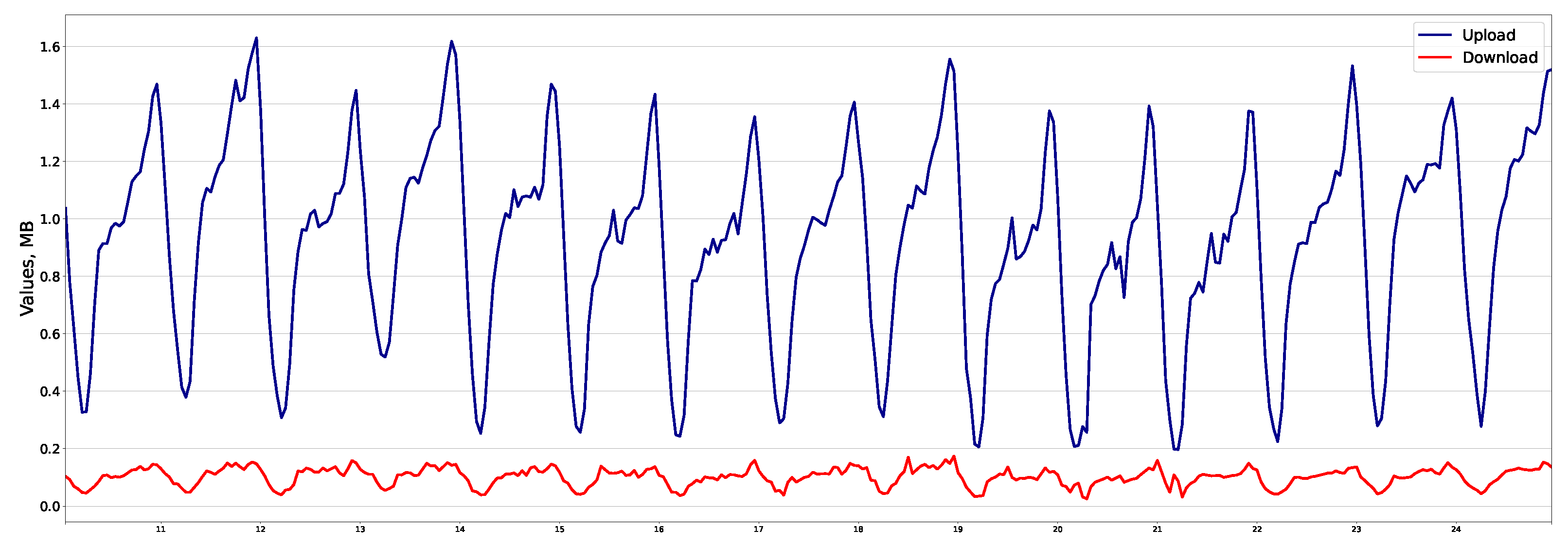
2.2. Total Traffic Behavior

Let us examine traffic behavior in this study.

Table 5. Descriptive statistics for total traffic.

	Upload	Download
Mean	$0.5442475$	$0.05518938$
Standard deviation	$5.322763$	$1.702829$
Minimum	0	0
Mode	$0.000029$	$0.00001$
Maximum	$2324.251$	$1337.792$

provides further insight with descriptive statistics. For a specific user and application, the traffic can only flow in one direction. Therefore, there cannot be any upload traffic with non-zero download and vice versa, resulting in the minimum values of 0 in Table 5.

Specifically, let us consider upload traffic. The standard deviation is $5.322763$, and the mean is $0.5442475$. These values suggest that the ratio of the standard deviation to the array values of the samples differs, indicating that the values are distributed over a wider range of data values. For download traffic, the situation is comparable: the standard deviation is $1.702829$, and the mean is $0.05518938$, with a significant difference between the array values.

To assess the relationship between upload and download traffic, we used Spearman’s rank correlation coefficient, or Spearman’s $\rho$ [18]. We chose this non-parametric method instead of the parametric Pearson method due to the fact that the Pearson criterion is applied to two quantitative indicators that have a linear relationship. Spearman’s method can be applied to any set of data without requiring additional preparation and processing of the values. Essentially, it allows for the determination of the strength of the relationship. For upload and download traffic with statistically significant differences at $\rho$ < 0.01, a correlation coefficient of 0.914 indicates a very high correlation strength between upload and download traffic.

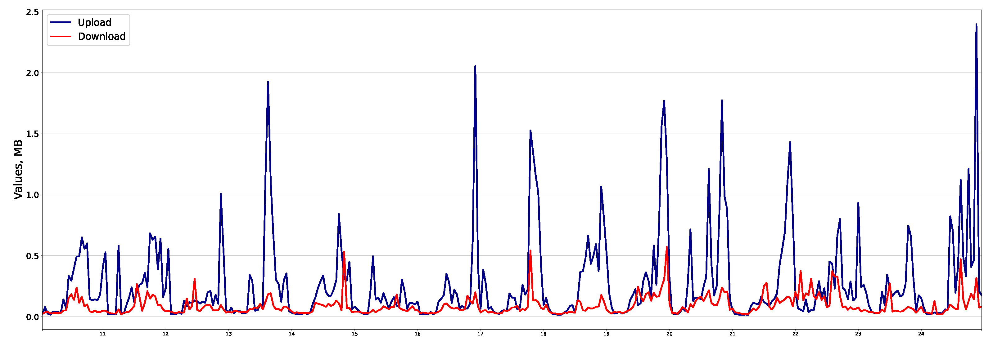
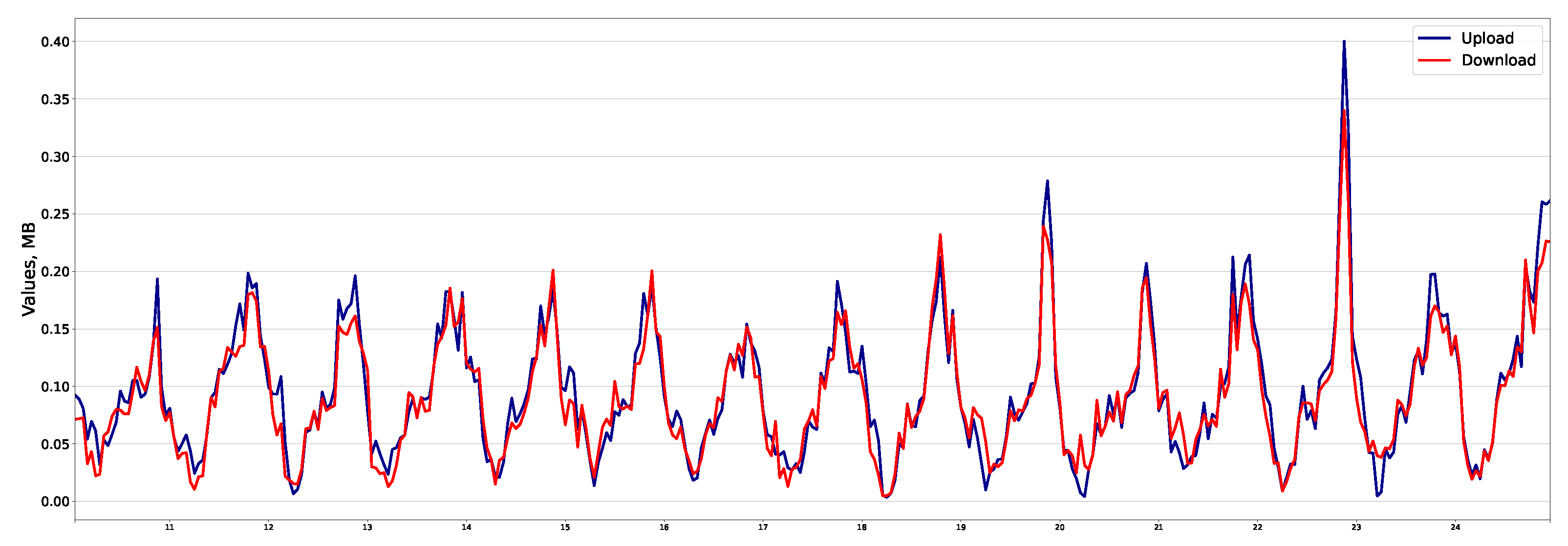
2.3. Traffic by Applications

Let us divide the application classes into three groups, as shown in

Table 6. Groups of applications.

Group	Applications
1. Time series is similar to the total traffic profile and seasonal	Others, Streaming Applications, Web Applications
2. Time series is not similar to the total traffic profile and non-seasonal with outliers	DB Transactions, File Systems, File Transfer, Games, Mail, Music Streaming, P2P Applications, Security, Terminals
3. Time series is not similar to the total traffic profile and seasonal	Instant Messaging Applications, Legacy Protocols, VoIP, Network Operation

. Figure 1, Figure 2 and Figure 3 illustrate the traffic profile in each group. Group No. 1 (Figure 1) is similar to the total traffic profile, and the time series is seasonal. For example, for “Web applications”, the correlation coefficient for upload and download traffic is 0.961. Group No. 2 (Figure 2) is not similar to the total traffic profile and is non-seasonal with outliers. In “Terminals” application, the correlation coefficient is 0.935. Group No. 3 (Figure 3) is not similar to the total traffic profile and is seasonal. For example, in “VoIP”, the coefficient is 0.708.

3. Statistical Models for Forecasting Traffic

In this section, we provide a description and formulas for two models that we will use for forecasting mobile network traffic: the SARIMA and Holt-Winters models.

Table 7. Main notation.

Parameter	Description
Time series parameters
$x_t$	Time series of data
$y_t$	Forecast value of $x_t$
SARIMA model parameters
p	Order of the non-seasonal AR part
d	Degree of differencing for the non-seasonal part
q	Order of the non-seasonal MA part
P	Order of the seasonal AR part
D	Degree of differencing for the seasonal part
Q	Order of the seasonal MA part
m	Number of periods in each season
$L{x}_t=x_{t-1},L^i{x}_t=x_{t-i}$	Lag operator
${\epsilon }_t$	Error terms
${\varphi }_i$	Parameters of the non-seasonal AR part
${\theta }_i$	Parameters of the non-seasonal MA part
${\Phi }_i$	Parameters of the seasonal AR part
${\Theta }_i$	Parameters of the seasonal MA part
Holt-Winters model parameters
$s_t$	Smoothed value of $x_t$
$b_t$	Estimate of the trend
$c_t$	Seasonal change factor
$\alpha$	Data smoothing factor
$\beta$	Trend smoothing factor
$\gamma$	Seasonal change smoothing factor

includes the notations used for the parameters of the SARIMA and Holt-Winters models.

3.1. Seasonal ARIMA Model

The seasonal autoregressive integrated moving average (SARIMA) model is an extension of the ARIMA model that explicitly supports univariate time series data with a seasonal component [45,46,47]. The model comprises three hyperparameters that define the autoregressive (AR), integrated (I), and moving average (MA) for the non-seasonal component of the time series, as well as an additional hyperparameter for the seasonal period (S). The model is denoted as SARIMA $(p,d,q){(P,D,Q)}_m$, where the first three parameters $(p,d,q)$ refer to the non-seasonal part of the model (ARIMA), whereas the last parameters ${(P,D,Q)}_m$ represent the seasonal part. Specifically, p is the order (number of time lags) of the non-seasonal AR part, d is the degree of differencing (the number of times the data have had past values subtracted) for the non-seasonal part, q is the order of the non-seasonal MA part, P is the order of the seasonal AR part, D is the degree of differencing for the seasonal part, Q is the order of the seasonal MA part, and m is the number of periods in each season.

Given a time series of data $x_i$, $i=0,\dots ,t-1$, in order to calculate the forecast value of $y_t=x_t$ at time t, the SARIMA model is used and written as

$$\begin{array}{cc}\left(1-\sum _{i=1}^p{\varphi }_i{L}^i\right)\left(1-\sum _{i=1}^P{\Phi }_i{L}^{im}\right){\left(1-L\right)}^d{\left(1-L^m\right)}^D{x}_t\hfill & \\ \hfill =& \left(1+\sum _{i=1}^q{\theta }_i{L}^i\right)\left(1+\sum _{i=1}^Q{\Theta }_i{L}^{im}\right){\epsilon }_t,\hfill \end{array}$$

where $L{x}_t=x_{t-1}$ and $L^i{x}_t=x_{t-i}$ represent the lag operator, ${\epsilon }_t$ are the error terms, ${\varphi }_i$ are the parameters of the non-seasonal AR part of the model, ${\theta }_i$ are the parameters of the non-seasonal MA part, ${\Phi }_i$ are the parameters of the seasonal AR part, ${\Theta }_i$ are the parameters of the seasonal MA part.

3.2. Holt-Winters Model

The Holt-Winters model, also known as triple exponential smoothing, is used to predict time series data that exhibit both trend and seasonal variations [18,46,47]. There are different types of trends and seasonality: additive and multiplicative in nature, meaning linear and exponential, respectively.

Given a time series of data $x_i$, $i=0,\dots ,t-1$, let us denote the forecast value of $x_t$ at time t as $y_t$, the smoothed value of $x_t$ at time t as $s_t$, the estimate of the trend at time t as $b_t$, and the seasonal change factor at time t as $c_t$. Depending on the types of trend and seasonality, the following formulas represent the Holt-Winters model [48]:

• additive (linear) trend and additive (linear) seasonality

  $$\begin{array}{cc}\hfill y_{t+h}& =s_t+h{b}_t+c_{t+h-m\left(\lfloor \frac{h-1}{m}\rfloor +1\right)},\hfill \\ \hfill s_t& =\alpha (x_t-c_{t-m})+(1-\alpha )(s_{t-1}+b_{t-1}),\hfill \\ \hfill b_t& =\beta (s_t-s_{t-1})+(1-\beta )b_{t-1},\hfill \\ \hfill c_t& =\gamma (x_t-s_t)+(1-\gamma )c_{t-m};\hfill \end{array}$$
• multiplicative (exponential) trend and additive (linear) seasonality

  $$\begin{array}{cc}\hfill y_{t+h}& =s_t·h{b}_t+c_{t+h-m\left(\lfloor \frac{h-1}{m}\rfloor +1\right)},\hfill \\ \hfill s_t& =\alpha (x_t-c_{t-m})+(1-\alpha )s_{t-1}·b_{t-1},\hfill \\ \hfill b_t& =\beta \frac{s_t}{s_{t-1}}+(1-\beta )b_{t-1},\hfill \\ \hfill c_t& =\gamma (x_t-s_t)+(1-\gamma )c_{t-m};\hfill \end{array}$$
• additive (linear) trend and multiplicative (exponential) seasonality

  $$\begin{array}{cc}\hfill y_{t+h}& =\left(s_t+h{b}_t\right)·c_{t+h-m\left(\lfloor \frac{h-1}{m}\rfloor +1\right)},\hfill \\ \hfill s_t& =\alpha \frac{x_t}{c_{t-m}}+(1-\alpha )(s_{t-1}+b_{t-1}),\hfill \\ \hfill b_t& =\beta (s_t-s_{t-1})+(1-\beta )b_{t-1},\hfill \\ \hfill c_t& =\gamma \frac{x_t}{s_t}+(1-\gamma )c_{t-m};\hfill \end{array}$$
• multiplicative (exponential) trend and multiplicative (exponential) seasonality

  $$\begin{array}{cc}\hfill y_{t+h}& =s_t·h{b}_t·c_{t+h-m\left(\lfloor \frac{h-1}{m}\rfloor +1\right)},\hfill \\ \hfill s_t& =\alpha \frac{x_t}{c_{t-m}}+(1-\alpha )s_{t-1}·b_{t-1},\hfill \\ \hfill b_t& =\beta \frac{s_t}{s_{t-1}}+(1-\beta )b_{t-1},\hfill \\ \hfill c_t& =\gamma \frac{x_t}{s_t}+(1-\gamma )c_{t-m};\hfill \end{array}$$

where $\alpha$ is the data smoothing factor, $\beta$ is the trend smoothing factor, and $\gamma$ is the seasonal change smoothing factor.

3.3. Preliminary Checks

Before applying the SARIMA and Holt-Winters models, some preliminary checks should be conducted [49]. Both models require that the data series exhibit seasonality. For this purpose, the STL (seasonal and trend decomposition using Loess) decomposition [50] can be employed. The seasonal period is 24 h and is associated with user activity. The seasonal variation around each level appears to increase proportionally with the current levels. Therefore, seasonality may be multiplicative. Regarding the trend, there are no significant changes in the lines, and their slopes are close to zero. Therefore, we may consider the trend as additive.

To verify the stationarity of the time series, we employed the ADF (Augmented Dickey–Fuller) test [51] and the KPSS (Kwiatkowski–Phillips–Schmidt–Shin) test. In both tests, the test statistic should be less than the significance level of $\alpha =0.05$. The ADF test assesses the null hypothesis that the time series is not stationary. For both upload and download traffic, the p-values are less than 0.05, with values of 0.00063973 and 0.000000725, respectively. The null hypothesis for the KPSS test is opposite to that of the ADF test. The p-value for the KPSS test is 0.1 in both cases, which exceeds $\alpha =0.05$. Therefore, we can conclude that the time series is stationary.

4. Forecasting Download and Upload Traffic

In this section, we will begin with discussing the metrics used to evaluate the models, and then move on to forecasting download and upload traffic.

4.1. Evaluation Metrics

The first step is to choose the parameters for the models. For the SARIMA model, we choose the parameters $p,d,q,P,D,Q$ using the Akaike information criterion (AIC) [46] in order to minimize it. Specifically, we use the following equation for AIC:

$$\mathrm{AIC}=2k-2log\left(L\right)=2(p+q+P+Q)-2log\left(L\right),$$

where k is the number of estimated parameters in the model, and L is the maximized value of the likelihood function for the model. For the Holt-Winters model, the equations depend on the types of trend and seasonality, namely, additive and multiplicative. We perform brute force checks to determine the appropriate equations.

The second step is to compare different models. We use typical evaluation metrics [52,53] such as mean squared error (MSE), root mean square error (RMSE), mean absolute error (MAE), mean absolute percentage error (MAPE), and mean squared logarithmic error (MSLE).

Table 8. Metrics for traffic forecast evaluation.

Metric	Formula
Mean squared error (MSE)	$$\frac{1}{n}\sum _{t=1}^n{\left(x_t-y_t\right)}^2$$
Root mean square error (RMSE)	$$\sqrt{\frac{1}{n}\sum _{t=1}^n{\left(x_t-y_t\right)}^2}$$
Mean absolute error (MAE)	$$\frac{1}{n}\sum _{t=1}^n\left|x_t-y_t\right|$$
Mean absolute percentage error (MAPE)	$$\frac{1}{n}\sum _{t=1}^n\left|\frac{x_t-y_t}{x_t}\right|·100\%$$
Mean squared logarithmic error (MSLE)	$$\frac{1}{n}\sum _{t=1}^n{\left[log(x_t+1)-log(y_t+1)\right]}^2$$

provides a summary of these metrics. In our notation, $x_t$ represents the time series data and $y_t$ denotes the forecasted value of $x_t$.

The dataset was normalized and divided into a training dataset of 13 days and testing datasets of 2 days, which is approximately 13%. We used Python for programming and its modules statsmodels and pmdarima.

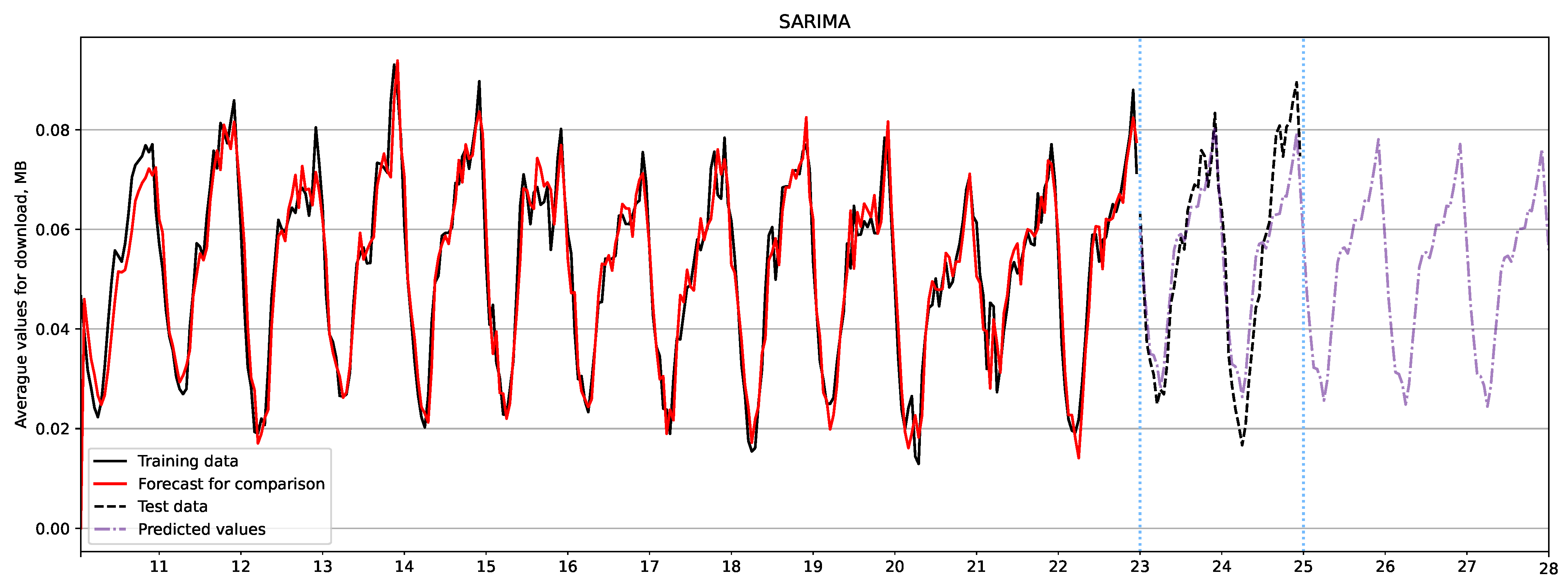
4.2. Download Traffic

For download traffic, the parameters for the SARIMA model are as follows:

$$\mathrm{SARIMA}(2,0,1){(0,0,2)}_{24}.$$

For the Holt-Winters model, the trend appears to be multiplicative and the seasonality additive.

Figure 4 and Figure 5 show three-day forecast plots for download traffic using the SARIMA and Holt-Winters models, respectively. The black line represents the training data, the black dashed line represents the test data, the forecast is shown in purple, and the red line shows the forecast for comparison with the actual data.

Table 9. Metrics for download traffic forecast evaluation.

Metric	SARIMA Model	Holt-Winters Model
MSE	0.0181	0.00021
RMSE	0.0181	0.0145
MAE	0.01513	0.01217
MAPE	15%	11.2%
MSLE	0.000258	0.000163

summarizes the evaluation metrics that demonstrate the superiority of the Holt-Winters model in forecasting download traffic.

4.3. Upload Traffic

For upload traffic, the parameters for the SARIMA model are as follows:

$$\mathrm{SARIMA}(3,0,1){(2,0,2)}_{24}.$$

For the Holt-Winters model, the trend appears also to be multiplicative and the seasonality additive.

The forecast for upload traffic is shown in Figure 6 and Figure 7 using the SARIMA and Holt-Winters models, respectively. By comparing the test and forecast data, we can conclude that the dynamics of the forecast peaks for upload traffic do not repeat the test values. Additionally, the fluctuations exhibit pronounced general seasonality. However, if we consider day 24, the SARIMA model shows better results as it accurately predicts the peak in the data. On the other hand, the Holt-Winters model assumes peaks in days after day 24, resulting in fluctuations that have pronounced overall seasonality and are more similar to the test data. Based on the results in

Table 10. Metrics for upload traffic forecast evaluation.

Metric	SARIMA Model	Holt-Winters Model
MSE	0.00004	0.00015
RMSE	0.006	0.0123
MAE	0.0046	0.0099
MAPE	4.17%	9.9%
MSLE	0.00003	0.000118

, it can be concluded that the SARIMA model is more accurate in predicting upload traffic in our case.

4.4. Discussion

This study aimed to examine the effectiveness of using SARIMA and Holt-Winters models for short-term forecasting of mobile network traffic. The findings of the study indicate that both models can yield valuable insights for predicting future traffic in mobile networks. The SARIMA model has been recognized for its capability to capture temporal patterns in time series data. It exhibited effectiveness in capturing short-term fluctuations and trends in mobile network traffic. Additionally, the Holt-Winters seasonal model, designed to account for the inherent seasonality in time series data, was also explored. By incorporating seasonal components such as trend and seasonality, the Holt-Winters model successfully captured cyclical patterns of mobile network traffic.

To assess the forecast results, we computed various evaluation metrics, including MSE, RMSE, MAE, MAPE, and MSLE. The results, presented in Table 9 and Table 10, demonstrated the suitability of each model for different datasets. In an effort to facilitate comparison between the predicted and test data, distinct lines were plotted on Figure 8 with four lines representing the absolute error indicators for both models and the traffic directions.

5. Conclusions

The number of users and equipment is growing extremely quickly, and telecom operators need to understand the demand for different types of applications in next-generation networks. The ability to predict such demand would help service providers make better offers to customers. This paper has explored the use of statistical methods of data analysis in the context of 5G networks. The main objective of this study was to analyze mobile network traffic and develop forecasting models for traffic profiles. Two statistical models, SARIMA and Holt-Winters, were constructed and evaluated for this purpose. The results demonstrate that both models effectively predict the average values of upload and download traffic within a certain range. However, it was observed that the Holt-Winters model is better suited for forecasting download traffic profiles, while SARIMA is more suitable for upload traffic profiles.

From our numerical analysis, we found that each statistical method has its own specifications. There is no universality, as each dataset requires its own approach. For example, the MAPE for download traffic was 11.2% for SARIMA and 15% for Holt-Winters. However, the Holt-Winters model was better suited for upload traffic, with a MAPE of 4.17% compared to 9.9% for SARIMA and Holt-Winters, respectively. Additionally, we observed that the MSE metric for download traffic was 86 times less for the Holt-Winters model (0.00021) compared to SARIMA (0.0181). Conversely, for upload traffic, the MSE was almost four times less for SARIMA (0.00004) compared to Holt-Winters (0.0015).

Future studies will focus on combining statistical models with machine learning methods for more precise forecasts, as well as anomaly detection. By implementing such techniques, we aim to enhance the accuracy and reliability of traffic forecasting in 5G networks. These findings contribute to the growing body of knowledge surrounding the utilization of data analysis methods in the field of telecommunications.

References

1. Giordani, M.; Polese, M.; Mezzavilla, M.; Rangan, S.; Zorzi, M. Toward 6G Networks: Use Cases and Technologies. IEEE Commun. Mag. 2020, 58, 55–61. [Google Scholar] [CrossRef]
2. Saad, W.; Bennis, M.; Chen, M. A Vision of 6G Wireless Systems: Applications, Trends, Technologies, and Open Research Problems. IEEE Netw. 2020, 34, 134–142. [Google Scholar] [CrossRef]
3. Campos, R.; Ricardo, M.; Pouttu, A.; Correia, L. Wireless Technologies Towards 6G. Eurasip J. Wirel. Commun. Netw. 2023, 2023. [Google Scholar] [CrossRef]
4. Kochetkov, D.; Vuković, D.; Sadekov, N.; Levkiv, H. Smart Cities and 5G Networks: An Emerging Technological Area? J. Geogr. Inst. Jovan Cvijic SASA 2019, 69, 289–295. [Google Scholar] [CrossRef]
5. Kochetkov, D.; Almaganbetov, M. Using Patent Landscapes for Technology Benchmarking: A Case of 5G Networks. Adv. Syst. Sci. Appl. 2021, 21, 20–28. [Google Scholar] [CrossRef]
6. Ruiz, S.; Ahmadi, H.; Gardašević, G.; Haddad, Y.; Katzis, K.; Grazioso, P.; Petrini, V.; Reichman, A.; Ozdemir, M.; Velez, F.; et al. 5G and Beyond Networks; Elsevier: Amsterdam, The Netherlands, 2021; pp. 141–186. [Google Scholar] [CrossRef]
7. Moltchanov, D.; Sopin, E.; Begishev, V.; Samuylov, A.; Koucheryavy, Y.; Samouylov, K. A Tutorial on Mathematical Modeling of 5G/6G Millimeter Wave and Terahertz Cellular Systems. IEEE Commun. Surv. Tutorials 2022, 24, 1072–1116. [Google Scholar] [CrossRef]
8. Kondratyeva, A.; Ivanova, D.; Begishev, V.; Markova, E.; Mokrov, E.; Gaidamaka, Y.; Samouylov, K. Characterization of Dynamic Blockage Probability in Industrial Millimeter Wave 5G Deployments. Future Internet 2022, 14, 193. [Google Scholar] [CrossRef]
9. Mokrov, E.; Samouylov, K. Performance Assessment and Comparison of Deployment Options for 5G Millimeter Wave Systems. Future Internet 2023, 15, 60. [Google Scholar] [CrossRef]
10. ITU-T. SERIES Y: Global Information Infrastructure, Internet Protocol Aspects, Next-Generation Networks, Internet of Things and Smart Cities; Technical Recommendation (TR) Y.3651; ITU Telecommunication Standardization Sector (ITU-T): Geneva, Switzerland, 2018. [Google Scholar]
11. 3GPP. 5G System (5GS); Study on Traffic Characteristics and Performance Requirements for AI/ML Model Transfer; Technical Report (TR) 22.874; Release 18, V18.2.0; 3rd Generation Partnership Project (3GPP): Valbonne, France, 2017. [Google Scholar]
12. ITU-T. SERIES Y: Global Information Infrastructure, Internet Protocol Aspects, Next-Generation Networks, Internet of Things and Smart Cities; Technical Recommendation (TR) Y.3602; ITU Telecommunication Standardization Sector (ITU-T): Geneva, Switzerland, 2022. [Google Scholar]
13. Cisco. Spend Less Time Managing Your Network. 2022. Available online: https://www.cisco.com/site/us/en/products/networking/dna-center-platform/index.html (accessed on 1 June 2022).
14. Chen, A.; Law, J.; Aibin, M. A Survey on Traffic Prediction Techniques Using Artificial Intelligence for Communication Networks. Telecom 2021, 2, 518–535. [Google Scholar] [CrossRef]
15. Efron, B.; Hastie, T. Computer Age Statistical Inference: Algorithms, Evidence, and Data Science; Cambridge University Press: Cambridge, UK, 2016; pp. 1–475. [Google Scholar] [CrossRef]
16. Jiang, W. Cellular Traffic Prediction with Machine Learning: A Survey. Expert Syst. Appl. 2022, 201, 117163. [Google Scholar] [CrossRef]
17. Gorshenin, A.; Kuzmin, V. Statistical Feature Construction for Forecasting Accuracy Increase and Its Applications in Neural Network Based Analysis. Mathematics 2022, 10, 589. [Google Scholar] [CrossRef]
18. Downey, A.; Loukides, M.; Blanchette, M.; Demarest, R. Think Stats: Exploratory Data Analysis; O’Reilly Media: Sebastopol, CA, USA, 2014; pp. 1–223. [Google Scholar]
19. Gorshenin, A.; Shcherbinina, A. Efficiency of the Method for Detecting Normal Mixture Signals with Pre-Estimated Gaussian Mixture Noise. Pattern Recognit. Image Anal. 2020, 30, 470–479. [Google Scholar] [CrossRef]
20. Gorshenin, A.; Kazakov, I.; Korolev, V. On the Convergence of Median Versions of the Expectation-Maximization Algorithm for the Separation of Finite Normal Mixtures. J. Math. Sci. 2022, 267, 92–98. [Google Scholar] [CrossRef]
21. Xu, F.; Lin, Y.; Huang, J.; Wu, D.; Shi, H.; Song, J.; Li, Y. Big Data Driven Mobile Traffic Understanding and Forecasting: A Time Series Approach. IEEE Trans. Serv. Comput. 2016, 9, 796–805. [Google Scholar] [CrossRef]
22. Stepanov, N.; Alekseeva, D.; Ometov, A.; Lohan, E. Applying Machine Learning to LTE Traffic Prediction: Comparison of Bagging, Random Forest, and SVM. In Proceedings of the 12th International Congress on Ultra Modern Telecommunications and Control Systems and Workshops, ICUMT 2020, Brno, Czech Republic, 5–7 October 2020; pp. 119–123. [Google Scholar] [CrossRef]
23. Ma, T.; Antoniou, C.; Toledo, T. Hybrid Machine Learning Algorithm and Statistical Time Series Model for Network-Wide Traffic Forecast. Transp. Res. Part Emerg. Technol. 2020, 111, 352–372. [Google Scholar] [CrossRef]
24. Lens Shiang, E.; Chien, W.C.; Lai, C.F.; Chao, H.C. Gated Recurrent Unit Network-based Cellular Traffic Prediction. In Proceedings of the 34th International Conference on Information Networking, ICOIN 2020, Barcelona, Spain, 7–10 January 2020; pp. 471–476. [Google Scholar] [CrossRef]
25. Zhaowei, Q.; Haitao, L.; Zhihui, L.; Tao, Z. Short-Term Traffic Flow Forecasting Method with M-B-LSTM Hybrid Network. IEEE Trans. Intell. Transp. Syst. 2022, 23, 225–235. [Google Scholar] [CrossRef]
26. Shan, M.; Yan, Q.; Huang, S.; Wang, Y. Prediction and Analysis of Telemetry Data Based on LSTM Network. In Proceedings of the 2nd International Conference on Computer Network, Electronic and Automation, ICCNEA 2019, Xi’an; China, 27–29 September 2019; pp. 155–159. [Google Scholar] [CrossRef]
27. Syam, R.F.; Girsang, A.S. Bandwidth Provisioning for 4G Mobile Network Using Hybrid ARIMA-LSTM Based Traffic Forecasting. Int. J. Eng. Trends Technol. 2021, 69, 235–241. [Google Scholar] [CrossRef]
28. Azari, A.; Salehi, F.; Papapetrou, P.; Cavdar, C. Energy and Resource Efficiency by User Traffic Prediction and Classification in Cellular Networks. IEEE Trans. Green Commun. Netw. 2022, 6, 1082–1095. [Google Scholar] [CrossRef]
29. Tran, Q.T.; Hao, L.; Trinh, Q.K. Cellular Network Traffic Prediction Using Exponential Smoothing Methods. J. Inf. Commun. Technol. 2019, 18, 1–18. [Google Scholar] [CrossRef]
30. Peng, Y.; Lei, M.; Li, J.B.; Peng, X.Y. A Novel Hybridization of Echo State Networks and Multiplicative Seasonal ARIMA Model for Mobile Communication Traffic Series Forecasting. Neural Comput. Appl. 2014, 24, 883–890. [Google Scholar] [CrossRef]
31. Kurri, V.; Raja, V.; Prakasam, P. Cellular Traffic Prediction on Blockchain-Based Mobile Networks Using LSTM Model in 4G LTE Network. Peer-to-Peer Netw. Appl. 2021, 14, 1088–1105. [Google Scholar] [CrossRef]
32. Oduro-Gyimah, F.K.; Boateng, K.O. Using Autoregressive Integrated Moving Average Models in the Analysis and Forecasting of Mobile Network Traffic Data. J. Eng. Res. 2019, 7, 1–9. [Google Scholar] [CrossRef]
33. Céspedes, J.E.S.; Rodríguez, Y.G.; Sarmiento, D.A.L. Development of An Univariate Method for Predicting Traffic Behaviour in Wireless Networks through Statistical Models. Int. J. Eng. Technol. 2015, 7, 27–36. [Google Scholar]
34. Bastos, J.A. Forecasting the Capacity of Mobile Networks. Telecommun. Syst. 2019, 72, 231–242. [Google Scholar] [CrossRef]
35. Ak, E.; Canberk, B. Forecasting Quality of Service for Next-Generation Data-Driven WiFi6 Campus Networks. IEEE Trans. Netw. Serv. Manag. 2021, 18, 4744–4755. [Google Scholar] [CrossRef]
36. Sone, S.P.; Lehtomäki, J.J.; Khan, Z. Wireless Traffic Usage Forecasting Using Real Enterprise Network Data: Analysis and Methods. IEEE Open J. Commun. Soc. 2020, 1, 777–797. [Google Scholar] [CrossRef]
37. Shayea, I.; Alhammadi, A.; El-Saleh, A.A.; Hassan, W.H.; Mohamad, H.; Ergen, M. Time Series Forecasting Model of Future Spectrum Demands for Mobile Broadband Networks in Malaysia, Turkey, and Oman. Alex. Eng. J. 2022, 61, 8051–8067. [Google Scholar] [CrossRef]
38. Gijón, C.; Toril, M.; Luna-Ramírez, S.; Marí-Altozano, M.L.; Ruiz-Avilés, J.M. Long-Term Data Traffic Forecasting for Network Dimensioning in LTE with Short Time Series. Electronics 2021, 10, 1151. [Google Scholar] [CrossRef]
39. Li, Y.; Wang, Y. Mobile Virtual Reality Rail Traffic Congestion Prediction Algorithm Based on Convolutional Neural Network. Mob. Inf. Syst. 2022, 2022, 2174208. [Google Scholar] [CrossRef]
40. Biernacki, A. Traffic Prediction Methods for Quality Improvement of Adaptive Video. Multimed. Syst. 2018, 24, 531–547. [Google Scholar] [CrossRef]
41. Yu, Q.; Jibin, L.; Jiang, L. An Improved ARIMA-Based Traffic Anomaly Detection Algorithm for Wireless Sensor Networks. Int. J. Distrib. Sens. Netw. 2016, 2016, 9653230. [Google Scholar] [CrossRef]
42. Feng, H.; Shu, Y.; Ma, M. WLAN Traffic Prediction Using Support Vector Machine. IEICE Trans. Commun. 2009, E92-B, 2915–2921. [Google Scholar] [CrossRef]
43. Yadav, R.K.; Balakrishnan, M. Comparative Evaluation of ARIMA and ANFIS for Modeling of Wireless Network Traffic Time Series. Eurasip J. Wirel. Commun. Netw. 2014, 2014, 15. [Google Scholar] [CrossRef]
44. Arifin, A.S.; Habibie, M.I. The Prediction of Mobile Data Traffic based on the ARIMA Model and Disruptive Formula in Industry 4.0: A Case Study in Jakarta, Indonesia. Telkomnika (Telecommun. Comput. Electron. Control) 2020, 18, 907–918. [Google Scholar] [CrossRef]
45. Box, G.; Jenkins, G.; Reinsel, G.; Ljung, G. Time Series Analysis: Forecasting and Control; Wiley: Hoboken, NJ, USA, 2015; pp. 1–712. [Google Scholar]
46. Cryer, J.; Chan, K. Time Series Analysis: With Applications in R; Springer: Berlin/Heidelberg, Germany, 2008; pp. 1–491. [Google Scholar]
47. Faverjon, C.; Berezowski, J. Choosing the Best Algorithm for Event Detection Based on the Intend Application: A Conceptual Framework for Syndromic Surveillance. J. Biomed. Inform. 2018, 85, 126–135. [Google Scholar] [CrossRef] [PubMed]
48. Hyndman, R.; Athanasopoulos, G. Forecasting: Principles and Practice; OTexts: Melbourne, Australia, 2021; pp. 1–442. [Google Scholar]
49. Miao, D.; Qin, X.; Wang, W. The Periodic Data Traffic Modeling based on Multiplicative Seasonal ARIMA Model. In Proceedings of the 6th International Conference on Wireless Communications and Signal Processing, WCSP 2014, Hefei, China, 23–25 October 2014. [Google Scholar] [CrossRef]
50. Cleveland, R.B.; Cleveland, W.S.; McRae, J.E.; Terpenning, I. STL: A Seasonal-Trend Decomposition Procedure Based on Loess. J. Off. Stat. 1990, 6, 3–73. [Google Scholar]
51. Kwiatkowski, D.; Phillips, P.; Schmidt, P.; Shin, Y. Testing the Null Hypothesis of Stationarity Against the Alternative of a Unit Root. How Sure are We that Economic Time Series Have a Unit Root? J. Econom. 1992, 54, 159–178. [Google Scholar] [CrossRef]
52. Efrosinin, D.; Kochetkova, I.; Stepanova, N.; Yarovslavtsev, A.; Samouylov, K.; Valentini, R. The Fourier Series Model for Predicting Sapflow Density Flux based on TreeTalker Monitoring System. Lect. Notes Comput. Sci. 2020, 12526, 198–209. [Google Scholar] [CrossRef]
53. Efrosinin, D.; Kochetkova, I.; Stepanova, N.; Yarovslavtsev, A.; Samouylov, K.; Valentini, R. Trees Classification based on Fourier Coefficients of the Sapflow Density Flux. Ann. Math. Informaticae 2021, 53, 109–123. [Google Scholar] [CrossRef]
Figure 1. “Web Applications” traffic (group of applications No. 1).
Futureinternet 15 00290 g001
Figure 2. “Terminals” traffic (group of applications No. 2).
Futureinternet 15 00290 g002
Figure 3. “VoIP” traffic (group of applications No. 3).
Futureinternet 15 00290 g003
Figure 4. Download traffic forecast using SARIMA model.
Futureinternet 15 00290 g004
Figure 5. Download traffic forecast using Holt-Winters model.
Futureinternet 15 00290 g005
Figure 6. Upload traffic forecast using SARIMA model.
Futureinternet 15 00290 g006
Figure 7. Upload traffic forecast using Holt-Winters model.
Futureinternet 15 00290 g007
Figure 8. Absolute error for traffic forecast.
Futureinternet 15 00290 g008