Intelligent Transmit Antenna Selection Schemes for High-Rate Fully Generalized Spatial Modulation

Abstract

The sixth-generation (6G) network is supposed to transmit significantly more data at much quicker rates than existing networks while meeting severe energy efficiency (EE) targets. The high-rate spatial modulation (SM) methods can be used to deal with these design metrics. SM uses transmit antenna selection (TAS) practices to improve the EE of the network. Although it is computationally intensive, free distance optimized TAS (FD-TAS) is the best for performing the average bit error rate (ABER). The present investigation aims to examine the effectiveness of various machine learning (ML)-assisted TAS practices, such as support vector machine (SVM), naïve Bayes (NB), K-nearest neighbor (KNN), and decision tree (DT), to the small-scale multiple-input multiple-output (MIMO)-based fully generalized spatial modulation (FGSM) system. To the best of our knowledge, there is no ML-based antenna selection schemes for high-rate FGSM. SVM-based TAS schemes achieve ∼71.1% classification accuracy, outperforming all other approaches. The ABER performance of each scheme is evaluated using a higher constellation order, along with various transmit antennas to achieve the target ABER of ${10}^{-5}$. By employing SVM for TAS, FGSM can achieve a minimal gain of ∼2.2 dB over FGSM without TAS (FGSM-NTAS). All TAS strategies based on ML perform better than FGSM-NTAS.

1. Introduction

In comparison to fifth-generation (5G) wireless communication networks, 6G networks are expected to have much higher spectral, energy, and cost efficiency, with higher data rates (in Tbps), latency reduced by a factor of ten, connection density increased by a factor of a hundred, and increased intelligence for full automation. Innovations such as index modulation (IM), reconfigurable intelligent surfaces (RISs), non-orthogonal multiple access (NOMA), and artificial intelligence (AI) will all be introduced into 6G networks to fulfill these overall objectives [1,2,3,4,5,6]. Massive MIMO designs can increase the spectral efficiency (SE) of 6G systems because of the higher frequencies and dense networks. In 6G, technologies like SM, RIS, NOMA, orbital angular momentum, and rate splitting multiple access have the potential to increase SE [7].

The energy efficiency (EE) of wireless networks may be enhanced by using four major approaches: (1) Resource allocation. Rather than maximizing throughput, the EE of the network is optimized by efficiently distributing resources [8]. (2) Instead of simply increasing the coverage area, the second option employs infrastructure nodes to increase the network’s EE. (3) Use renewable energy sources to power communication systems. (4) Design energy-efficient hardware solutions. In a network, IM and its derivatives can also be utilized to shoot up EE [9,10].

Massive MIMO is an essential technique for achieving the SE requirements of 5G. When adopting a multi-antenna system, two issues arise: inter-antenna synchronization (IAS) and inter-channel interference (ICI) [11]. With more radio frequency (RF) links, the hardware complexity of the system grows, lowering EE [12]. To overcome this problem, the concept of SM has been presented [9,10]. Because one antenna is functional at a time, the RF chain is simpler to handle in SM [9,10,11].

SM’s SE is given by

$${\alpha }_{SM}={log}_2\left(M\right)+{log}_2\left(N_{tx}\right),$$

(1)

where the number of transmit antennas and modulation order are denoted by $N_{tx}$ and M, respectively. The SE of SM is proportional to $lo{g}_2\left(N_{tx}\right)$. As a result, in order to enhance SE, a higher proportion of transmit antennas is required. SM cannot satisfy SE demands since only one antenna is simultaneously active [11]. High-rate SM variants are needed for future-generation networks to meet SE requirements [13]. The high-rate SM variants may transmit the same or distinct symbols at the same time across multiple antennas, depending on their operating principle. FGSM is a cutting-edge SM variant in which the transmitter uses just one or several, or all of its antennas for transmission [13]. As a result, the possible SE grows linearly with $N_{tx}$. Gudla V.V. et al. briefly discussed the system architecture and functioning theory of FGSM [13].

Transmit diversity gain could not be achieved in SM since only one antenna is fully functional at once [14,15,16,17]. The integration of TAS practices into SM improves its transmit diversity. The receiver decides on transmitter antenna subsets driven by the channel quality information (CQI). In ML, machines are taught new skills so that they may execute tasks on their own using data. In terms of planning and optimizing future-generation networks, ML plays a critical role. ML may be used to solve a wide range of technical difficulties in future-generation systems, including massive MIMO, NOMA, device-to-device (D2D) networks, etc. [2,3]. The present research performs TAS on FGSM using ML algorithms, and the effectiveness of these algorithms is evaluated using classification accuracy and ABER.

Related Work

The future-generation network demands improvements in EE and SE [1]. The SE of SM is proportional to $lo{g}_2\left(N_{tx}\right)$, which lowers the performance of SM in terms of SE [9,10]. To overcome this, high-rate versions of SM are developed [13]. FGSM is a high-rate variation of SM, where transmit antennas and SE are linearly related and could meet the expanding demands of 6G [13].

Lower-powered integrated circuits, antenna diversity, or a mix of the two, may be adopted to boost EE [18]. The traditional SM technique does not provide transmit diversity gain. TAS practices have been incorporated to boost the SM system’s transmit diversity gain [14]. TAS approaches are applied to overcome the cost and complexity challenges in massive MIMO systems [12]. Different massive MIMO configurations have shown that antenna selection can improve performance and lower RF costs [19]. For optimal channel utilization, a novel SM technique is developed by fusing transmit mode switching and adaptive modulation techniques [20]. The free distance (FD) strategy is computationally more expensive due to the requirement of simultaneously searching for antenna pairs and constellation orders that maximize the least FD. Although FD-TAS provides the best EE performance, its implementation is more challenging. The FD-TAS system has gained popularity and is used as a benchmark in many TAS-related articles [3,13,14,15,16,17,21].

A capacity-optimized antenna selection (COAS) technique is addressed in conjunction with FD-TAS, where the antenna subset with the most prominent channel capacity is chosen [13,14,15,17]. The correlation angle of two antennas is used to evaluate the TAS [13,16]. In this study, the antenna subset with the least correlation is prioritized. The capacity and correlation angle-based technique is proposed to enhance ABER performance [13] while increasing computing complexity. A partitioning strategy that relies on the capacity and correlation angle further reduces the system’s complexity [13]. Sub-optimal techniques are less efficient than FD-TAS when it comes to TAS in SM and its variants [13,14,15,16,17].

To save the computations offered by FD-TAS, nowadays data-driven approaches are utilized. TAS is a classification problem that can be solved using supervised ML algorithms. A pattern recognition-based approach is proposed for traditional MIMO [22]. This work is tested for 5000 samples with KNN and SVM algorithms. This work can be extended further to various supervised learning algorithms and larger datasets to boost the overall system performance. Two unique features of the channel space are the element norm of $\mathit{H}$ and element norm of ${\mathit{H}}^H\mathit{H}$, which are used to analyze the performance of these algorithms. The absolute of elements of $\mathit{H}$ is used to analyze NB- and SVM-based TAS algorithms in conventional MIMO architecture [23]. The purpose of this research is to demonstrate how ML can be utilized to enhance the security of MIMO architecture. In the future, other ML algorithms could be employed to carry out this research. In this example, the algorithms are only trained on 10,000 samples; nevertheless, this number can be increased to improve overall efficiency.

To solve power assignment problems in adaptive SM-MIMO, supervised ML algorithms and deep neural networks (DNNs) are proposed and implemented [24]. The ABER performance in this work can be enhanced by extending the training data beyond 2000 feature label pairs. Other features, such as the angle of elements of $\mathit{H}$, real and imaginary parts of elements of $\mathit{H}$, etc., can be used as attributes to obtain better results. TAS as a classification problem is addressed using DNN and SVM for SM [25]. To construct the models, the channel gain and correlation properties of the column space of $\mathit{H}$ are retrieved. In this work, the comparison with other ML-based algorithms is not conducted with DNN and SVM. Altın, G. and Arslan, İ.A. selected both the transmit and receive antennas for SM using deep learning (DL) architectures [26]. We used DL-based algorithms to execute TAS for FGSM in [3] to meet the SE requirements and improve classification accuracy. The following is a list of research gaps identified:

• Most of these data-driven approaches are proposed and implemented for conventional MIMO and basic SM architectures.
• These data-driven strategies are neither proposed nor implemented for high-rate variants of SM.
• The TAS dataset is not available for FGSM in any of the repositories.

Listed below are the key contributions of this work:

• Through the repeated application of the FD-TAS algorithm, 4 different datasets (with a total of 10,000 entries) are produced. The dataset contains channel information for a variety of MIMO setups and antenna counts, as well as essential performance measures, like FD.
• For FGSM, four distinct supervised ML classification methods are used and tested for TAS: SVM, NB, KNN, and DT. The dataset size, the value of k, which is used in k-fold cross-validation, and parameters, such as the kernel type and hyperparameter K, are optimized to obtain the best results.
• The ABER and computational complexity of ML-based TAS approaches are contrasted to those of FGSM-NTAS and FD-TAS.
• An analysis of the proposed work is carried out in terms of SNR gain and classification accuracy.

The following is how the manuscript is structured: The principle of operation of FGSM is discussed elaborately in Section 2. The various ML algorithms used for TAS in the FGSM system are covered in Section 3. The proposed ML-based TAS practices and the conventional FD-TAS practice are subjected to a computational complexity study in Section 4. The ABER performance of ML-based algorithms is contrasted to the FD-TAS scheme in Section 5. Section 6 concludes the work by laying out future research directions.

2. System Model of FGSM Transceiver

FGSM is a high-rate version of SM that allows one, many, or all antennas to transmit the same symbol at the same instant. The SE is directly proportional to $N_{tx}$ as compared to SM, which improves the SE. This variation does not require that the number of transmit antennas be a power of two. The SE of FGSM is calculated as follows:

$${\alpha }_{FGSM}={log}_2\left(M\right)+\left(N_{tx}-1\right).$$

(2)

Consider the input bits [0 0 1 1] to comprehend FGSM mapping. An example with an SE of 4 bpcu (M = 4 and $N_{tx}$ = 3) is used to demonstrate FGSM mapping. As indicated in

Table 1. A sample mapping of the constellation bits for M = 4.

Data Bits	Index of Symbols	Transmitted Symbols
00	$s_1$	$-\frac{1}{\sqrt{2}}+\frac{1}{\sqrt{2}}j$
01	$s_2$	$-\frac{1}{\sqrt{2}}-\frac{1}{\sqrt{2}}j$
10	$s_3$	$\frac{1}{\sqrt{2}}+\frac{1}{\sqrt{2}}j$
11	$s_4$	$\frac{1}{\sqrt{2}}-\frac{1}{\sqrt{2}}j$

, the symbol $s_1$ is identified using the first ${log}_2\left(M\right)$ bits, i.e., [0 0]. It will be transmitted by the antenna pair (1, 2), which is selected using the next $\left(N_{tx}-1\right)$ bits, i.e., [1 1], as illustrated in

Table 2. A sample mapping of the spatial bits for $N_{tx}$ = 3.

Antenna Bits	Antenna Index
00	1
01	2
10	3
11	1,2

. For the given block of bits, the transmit vector generated is given by $\mathsf{\chi }={[-\frac{1}{\sqrt{2}}+\frac{1}{\sqrt{2}}j,-\frac{1}{\sqrt{2}}+\frac{1}{\sqrt{2}}j,0]}^T$. Consider an alternative set of bits [0 1 0 1], where the symbol $s_2$ is chosen by using the first ${log}_2\left(M\right)$ bits [0 1], as shown in Table 1. It will be transmitted by antenna 2, which is selected using the next $\left(N_{tx}-1\right)$ bits, i.e., [0 1], as illustrated in Table 2. For this set of bits, the vector to be transmitted is $\mathsf{\chi }={[0,-\frac{1}{\sqrt{2}}-\frac{1}{\sqrt{2}}j,0]}^T$.

The multipath channel $\mathit{H}$ and AWGN $\mathsf{\eta }$ influence the transmit vector $\mathsf{\chi }$. At the receiver end, the signal vector $\mathit{y}$ is stated as follows:

$$\underset{N_{rx}\times 1}{\underbrace{\mathit{y}}}=\underset{N_{rx}\times N_{tx}}{\underbrace{\mathit{H}}}\underset{N_{tx}\times 1}{\underbrace{\mathsf{\chi }}}+\underset{N_{rx}\times 1}{\underbrace{\mathsf{\eta }}}.$$

(3)

Consider the MIMO configuration $(N_{tx}=3,N_{rx}=4)$ with $M=4$. For the single antenna operational configuration explained earlier, the received signal vector could be expressed as follows:

$$\left[\begin{array}{c}{y}_1\\ y_2\\ y_3\\ y_4\end{array}\right]=\left[\begin{array}{ccc}{h}_{11}& h_{12}& h_{13}\\ h_{21}& h_{22}& h_{23}\\ h_{31}& h_{32}& h_{33}\\ h_{41}& h_{42}& h_{43}\end{array}\right]\left[\begin{array}{c}0\\ s_2\\ 0\end{array}\right]+\left[\begin{array}{c}{\eta }_1\\ {\eta }_2\\ {\eta }_3\\ {\eta }_4\end{array}\right].$$

(4)

It comes down to

$$\left[\begin{array}{c}{y}_1\\ y_2\\ y_3\\ y_4\end{array}\right]=\left[\begin{array}{c}{h}_{12}\\ h_{22}\\ h_{32}\\ h_{42}\end{array}\right]s_2+\left[\begin{array}{c}{\eta }_1\\ {\eta }_2\\ {\eta }_3\\ {\eta }_4\end{array}\right].$$

(5)

For single antenna operational case, the generalized form of the received signal is

$$\mathit{y}={\mathit{h}}_j{s}_m+\mathsf{\eta },j\in \left\{1,2,..N_{tx}\right\},m\in \left\{1,2,...M\right\}.$$

(6)

For the double antenna operational configuration explained earlier, the received signal vector could be indicated as follows:

$$\left[\begin{array}{c}{y}_1\\ y_2\\ y_3\\ y_4\end{array}\right]=\left[\begin{array}{ccc}{h}_{11}& h_{12}& h_{13}\\ h_{21}& h_{22}& h_{23}\\ h_{31}& h_{32}& h_{33}\\ h_{41}& h_{42}& h_{43}\end{array}\right]\left[\begin{array}{c}{s}_1\\ s_1\\ 0\end{array}\right]+\left[\begin{array}{c}{\eta }_1\\ {\eta }_2\\ {\eta }_3\\ {\eta }_4\end{array}\right].$$

(7)

It reduces to

$$\left[\begin{array}{c}{y}_1\\ y_2\\ y_3\\ y_4\end{array}\right]=\left[\begin{array}{c}{h}_{11}\\ h_{21}\\ h_{31}\\ h_{41}\end{array}\right]s_1+\left[\begin{array}{c}\hfill h_{12}\hfill \\ \hfill h_{22}\hfill \\ \hfill h_{32}\hfill \\ \hfill h_{42}\hfill \end{array}\right]s_1+\left[\begin{array}{c}{\eta }_1\\ {\eta }_2\\ {\eta }_3\\ {\eta }_4\end{array}\right].$$

(8)

For the double antenna operational case, the generalized form of the received signal is given by

$$\mathit{y}=\left({\mathit{h}}_{j_1}+{\mathit{h}}_{j_2}\right)s_m+\mathsf{\eta },j_1\ne j_2,j_1,j_2\in \left\{1,2,..N_{tx}\right\},m\in \left\{1,2,...M\right\}.$$

(9)

For the $N_A$ number of functional antennas, the generalized form of the received signal is represented as follows:

$$\mathit{y}=\left(\sum _{a=1}^{N_A}{\mathit{h}}_{j_a}\right)s_m+\mathsf{\eta },j_a\in \left\{1,2,..N_{tx}\right\},m\in \left\{1,2,...M\right\}.$$

(10)

When a receiver possesses perfect CQI, the maximum likelihood detection for the FGSM system with $N_A$ functional antennas is given by

$$\left[{\widehat{j}}_{a,a=1,2..N_A},{\widehat{s}}_m\right]=\underset{j_{a,a=1,2..N_A},s_m}{arg\; min}{∥\mathit{y}-\left(\sum _{a=1}^{N_A}{\mathit{h}}_{j_a}\right)s_m∥}^2.$$

(11)

3. Antenna Selection Schemes for FGSM

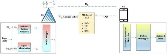
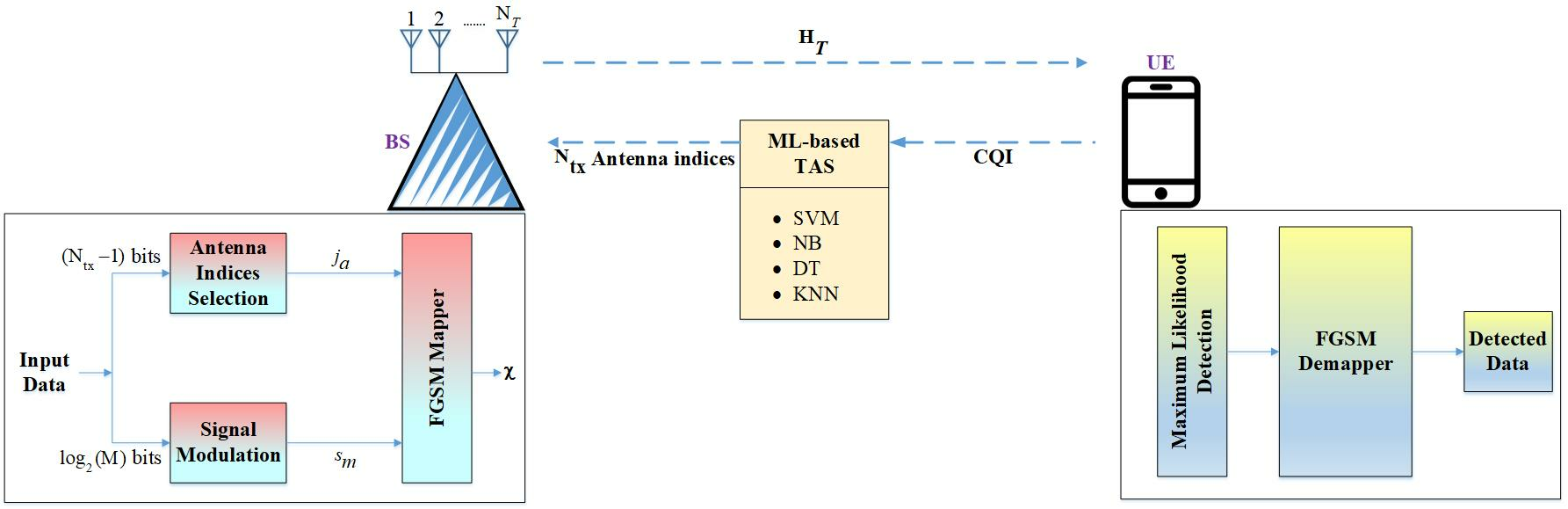
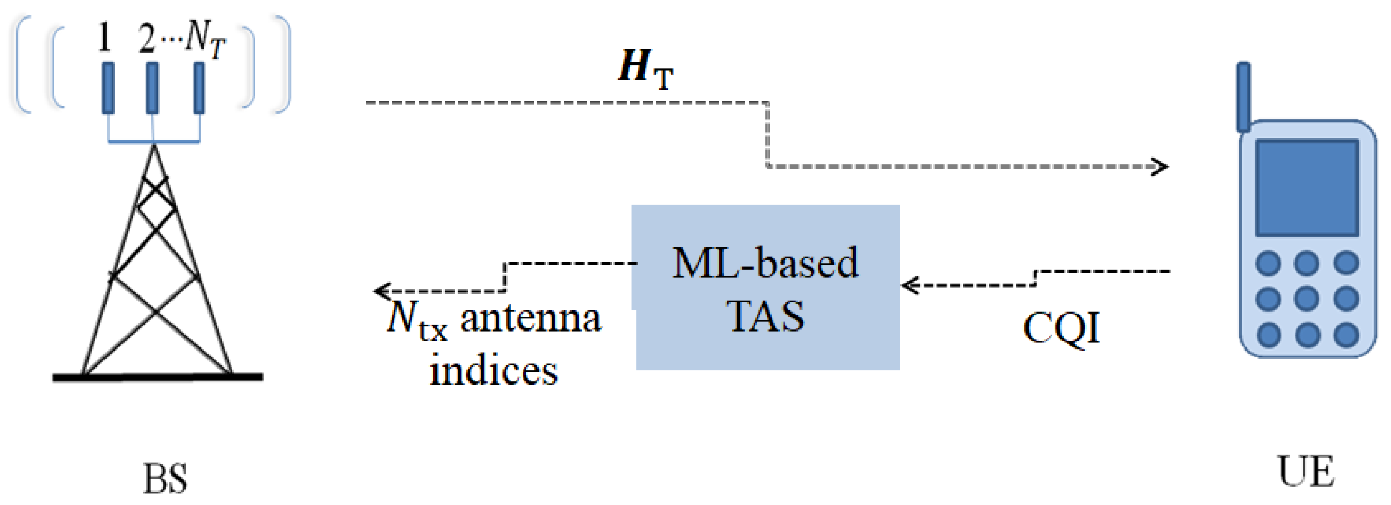
TAS for FGSM is schematically depicted in Figure 1. TAS drives up the transmit diversity in traditional MIMO and SM, as described in the literature review section. Let ${\mathit{H}}_T$ =$\left[{\mathit{h}}_1,{\mathit{h}}_2,\dots {\mathit{h}}_{N_T}\right]$∼$\mathbb{C}$$\mathcal{N}$$\left(0,I_{N_{rx}\times N_T}\right)$ be the channel matrix for a MIMO. Here, ${\mathit{h}}_1,{\mathit{h}}_2,\dots {\mathit{h}}_{N_T}$ are the column vectors of ${\mathit{H}}_T$. The TAS scheme is employed to select a subset from the candidate set S=$\left\{S_1,S_2,\cdots ,S_l,\cdots ,S_{N_s}\right\}$. $N_{tx}$ antennas are picked from $N_T$ antennas when the CQI is perfectly known to the user equipment (UE). There are $N_s$ possible antenna subsets, each with $N_{tx}$ antennas, as given below:

$$\begin{array}{c}{S}_1=\left\{1,2,\cdots ,N_{tx}\right\},\\ S_2=\left\{1,2,\cdots ,N_{tx}-1,N_{tx}+1\right\},\\ ⋮\\ S_{N_s}=\left\{N_T-N_{tx}+1,\cdots ,N_T\right\},\end{array}$$

(12)

where $S_l$ represents the lth possible transmit antenna subset. A low-rate feedback channel communicates the chosen subset antenna index to the base station (BS). The CQI feedback latency is assumed to be insignificant in this case. If $S_l$ is selected, then the signal received is expressed as follows:

$$\mathit{y}={\mathit{H}}_T^l\mathsf{\chi }+\mathsf{\eta },$$

(13)

where ${\mathit{H}}_T^l$ is the channel matrix corresponding to the selected set $S_l$. An example of the TAS candidate set mapping is illustrated in

Table 3. The TAS candidate set mapping for $N_T=4,N_{tx}=3,N_{rx}=4$.

TAS Candidate Set	Possible Antenna Subset
$S_1$	1,2,3
$S_2$	1,2,4
$S_3$	1,3,4
$S_4$	2,3,4

for $N_T=4,N_{tx}=3,\&N_{rx}=4$.

3.1. FD-TAS Based FGSM System

The purpose of FD-TAS is to find antenna pairs that optimize the least FD between the received constellations [3,13,14,15,16,17,21]. FD-TAS results in $\mathit{H}$ of size $N_{rx}\times N_{tx}$ from ${\mathit{H}}_T$ of size $N_{rx}\times N_T$. FD-TAS involves the following major steps:

Step 1: Compute the number of possible subsets $N_s$ = $\left(\begin{array}{c}{N}_T\\ N_{tx}\end{array}\right)$.

Step 2: Determine all feasible transmit vectors $\left(2^{{\alpha }_{FGSM}}\right)$ for every antenna subset.

Step 3: Determine the minimum FD for every antenna subset using

$$d_{min}\left({\mathit{H}}_T\right)=\underset{{\mathsf{\chi }}_i\ne {\mathsf{\chi }}_j}{min}{∥{\mathit{H}}_T\left({\mathsf{\chi }}_i-{\mathsf{\chi }}_j\right)∥}^2,$$

(14)

here, ${\mathsf{\chi }}_i,{\mathsf{\chi }}_j\in \mathbb{X}$ is the set of all feasible transmit vectors.

Step 4: Find an antenna subset that has the maximum FD.

$$\widehat{l}=\underset{l\in \left\{1,2,\dots N_s\right\}}{arg\; max}{d}_{min}\left({\mathit{H}}_T^l\right),$$

(15)

here, ${\mathit{H}}_T^l$= $\left[{\mathit{H}}_T^1,{\mathit{H}}_T^2,\dots {\mathit{H}}_T^{N_s}\right].$

Based on the antenna subset index obtained in step 4, the antenna indices and the associated channel matrix of size $N_{rx}\times N_{tx}$ are computed.

3.2. TAS Based on ML for FGSM

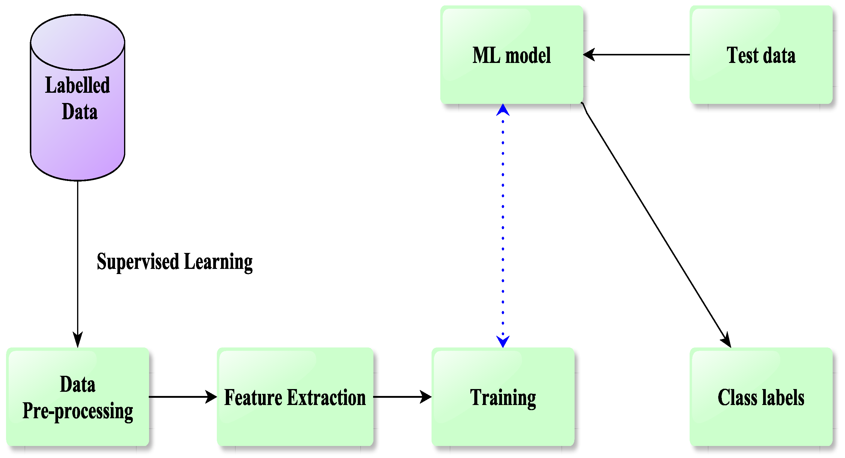
In this work, TAS in FGSM is carried out with the use of ML-based methods. An ML-based classification architecture is depicted in Figure 2. At first, source data are normalized using the mean normalization technique. Pre-processed data are then used to extract features. Several ML methods are then used to train the model using the chosen features and class labels. A trained model can be used to predict the class labels for new data using data that have not previously been fed into the system. The process for the execution of ML-based TAS for FGSM is shown in Figure 3. If CQI is present at the UE, the class labels obtained by the ML algorithms are utilized to choose $N_{tx}$ antennas from $N_T$. Algorithm 1 shows the processes that must be followed for ML-based TAS. This section also includes details on the dataset development process and the supervised algorithms that are employed.

Algorithm 1 Primary steps involved in ML-based TAS

1. Establish a mapping between the antenna subsets and class labels. 2. Pre-process the input data using the mean normalization technique. 3. Identify the key performance indicators (KPI) for each input sample. Find out the class label c on the basis of the KPI. 4. Employ the normalized feature matrix ${\widehat{\mathit{H}}}_T$ and the class label c to create a learning system utilizing SVM, NB, KNN, and DT algorithms. 5. The learning system converts the test channel ${\mathit{H}}_T^{new}$ to a normalized feature vector $\left({\mathit{f}}^{new}\right)$ and determines the class label c. 6. Compare the class label acquired in Step 5 with the map created in Step 1 to identify the antenna subset.

3.3. Generation of a Dataset

Elements of channel matrices are used to generate the training dataset. A multiclass classification technique is then used to divide the channel matrix into numerous corresponding classes, each of which represents the optimal antenna subset. ML methods are used to build the model. The developed models can also be used to predict the class labels of test data.

Four major steps are involved in the collection of the dataset: (1) Generation of training data. (2) Extraction of feature vectors. (3) Evaluation of KPI. (4) Use of the KPI information to obtain the class labels.

1.

Generation of training data.

To form the training data, the N number of channel matrices of size $N_{rx}\times N_T$ are randomly generated.

$$\mathbb{H}=\left[{\mathit{H}}_T^1,{\mathit{H}}_T^2,\cdots ,{\mathit{H}}_T^N\right].$$

(16)

2.

Extraction of feature vectors

The training performance is generally influenced by the feature vectors. In this work, four different features, i.e., $\left|h_{i,j}^n\right|$, $\measuredangle \left(h_{i,j}^n\right)$, channel gain ${\left|h_{i,j}^n\right|}^2$, and channel gain of every element of the correlation matrix ${\left|{{(\mathit{H}}_T^n)}^H{(\mathit{H}}_T^n)\right|}^2$, are considered to train the models. From each sample ${\mathit{H}}_T$, a feature of size $N_Q$$\left(N_{rx}\times N_T\right)$ is extracted. The process of extracting these four features is as follows:

(a)

$\left|h_{i,j}^n\right|$: The absolute value of each element of the channel matrix is considered as a dominating feature, which is used throughout this work. The extraction of the feature vector, in this case, is given as follows:

$${\mathit{f}}^n=\left[\left|h_{1,1}^n\right|,\cdots ,\left|h_{1,N_T}^n\right|,\cdots ,\left|h_{i,j}^n\right|,\cdots ,\left|h_{N_{rx},N_T}^n\right|\right],n\in \left\{1,2,...N\right\},$$

(17)

where $h_{i,j}^n$ is a $\left(i,j\right)$th complex element of ${\mathit{H}}_T^n$, whose absolute value is calculated as follows:

$$\left|h_{i,j}^n\right|=\sqrt{\Re {\left(h_{i,j}^n\right)}^2+\Im {\left(h_{i,j}^n\right)}^2}.$$

(18)

(b)

$\measuredangle \left(h_{i,j}^n\right)$: This is the second feature that is extracted to build the model from the elements of ${\mathit{H}}_T$. The feature vector is constructed as follows:

$${\mathit{f}}^n=\left[\measuredangle \left(h_{1,1}^n\right),\cdots ,\measuredangle \left(h_{1,N_T}^n\right),\cdots ,\measuredangle \left(h_{i,j}^n\right),\cdots ,\right.\left.\phantom{\int }\measuredangle \left(h_{N_{rx},N_T}^n\right)\right],n\in \left\{1,2,...N\right\},$$

(19)

where

$$\measuredangle \left(h_{i,j}^n\right)={tan}^{-1}\left(\frac{\Im \left(h_{i,j}^n\right)}{\Re \left(h_{i,j}^n\right)}\right).$$

(20)

(c)

Channel gain ${\left|h_{i,j}^n\right|}^2$: The channel gain of an individual element of the matrix is considered to be another feature to train the models whose feature vector is given by:

$${\mathit{f}}^n=\left[{\left|h_{1,1}^n\right|}^2,\cdots ,{\left|h_{1,N_T}^n\right|}^2,\cdots ,{\left|h_{i,j}^n\right|}^2,\cdots \right.\left.\phantom{\int }{\left|h_{N_{rx},N_T}^n\right|}^2\right],n\in \left\{1,2,...N\right\}.$$

(21)

(d)

Squared element norm of ${{(\mathit{H}}_T^n)}^H{(\mathit{H}}_T^n)$: In addition, the similarity between two distinct column vectors is a major feature. Similar column vectors introduce detection ambiguity while estimating the transmit antenna index. The feature vector extraction is conducted as follows:

$${\left|{{\mathit{H}}_T^n}^H{\mathit{H}}_T^n\right|}^2=\left[\begin{array}{c}{\left({\mathit{h}}_1^n\right)}^H\\ {\left({\mathit{h}}_2^n\right)}^H\\ ⋮\\ {\left({\mathit{h}}_{N_T}^n\right)}^H\end{array}\right]\left[\begin{array}{c}{\mathit{h}}_1^n{\mathit{h}}_2^n\cdots {\mathit{h}}_{N_T}^n\end{array}\right].$$

(22)

To avoid bias, features are normalized using

$${\overline{f}}^n\left(q\right)=\frac{f^n\left(q\right)-E\left[(\mathit{f}\left(q\right)\right]}{max\left(\mathit{f}\right(q\left)\right)-min\left(\right(\mathit{f}\left(q\right))},n=1,\dots ,N,q=1,\dots ,N_Q.$$

(23)

3.

Evaluation of KPI.

Input data samples are labeled using KPI. FD is considered as the KPI in this work, which is calculated using (14).

4.

Class labeling.

Associate each feature with a label. A transmit antenna subset S=$\left\{S_1,S_2,\cdots ,S_l,\cdots ,S_{N_s}\right\}$ is mapped to each feature vector. The feature vector corresponding to each channel matrix ${\widehat{\mathit{H}}}_T^n$ is mapped to label $c^n\in S$. Hence, the class label vector $\mathit{c}$=$\left[c^1,c^2,\cdots ,c^N\right]$.

3.4. ML Methods

This section examines four different supervised ML methods utilized for TAS.

3.4.1. SVM

An SVM model consists of a hyperplane containing representations of distinct classes in multidimensional space [22]. SVM will iteratively create the hyperplane in order to reduce errors. SVM divides datasets into classes in order to determine the best marginal hyperplane. TAS is a multiclass classification problem. The one-versus-one and one-versus-all (OVA) approaches are two common ways of creating multiclass SVM classifiers. This work looks at how OVA can be used to overcome the drawback of complexity in FD-TAS. It creates r binary SVMs for an R-class problem. Specifically, for TAS-assisted FGSM, R SVM models are generated as follows:

•

To address this two-class classification problem for the attribute label combinations $\left({\mathit{f}}^n,c^n\right)$, where n=1,$\dots ,N$, r $\in \left\{1,2,\dots ,R\right\}$, an R order SVM is constructed. In this case, ${\mathit{f}}^n$ represents the nth row of the normalized attribute matrix ${\widehat{\mathit{H}}}_T$. Samples belonging to the rth class are characterized by positive labels, while those belonging to the other classes are characterized by negative labels.

•

The following approach is used for solving the optimization problem for the two-class SVM:

$$\begin{array}{c}\underset{{\mathsf{\psi }}^r,z^r,{\lambda }^r}{min}\frac{1}{2}{\left({\mathsf{\psi }}^r\right)}^T{\mathsf{\psi }}^r+D^r{\displaystyle \sum _{n=1}^N}{\lambda }_n^r,\\ s.t.{\left({\mathsf{\psi }}^r\right)}^T\varphi \left({\mathit{f}}^n\right)+z^r\ge 1-{\lambda }_n^r,if{c}^n=r,\\ {\left({\mathsf{\psi }}^r\right)}^T\varphi \left({\mathit{f}}^n\right)+z^r\le -1+{\lambda }_n^r,if{c}^n\ne r,\\ {\lambda }_n^r\ge 0,r\in \left\{1,2,\dots ,R\right\},\end{array}$$

(24)

here, $z^r$ and ${\mathsf{\psi }}^r$ are linear parameters, $D^r$ and ${\lambda }_n^r$ are the regularization and penalty parameters, respectively, for rth SVM. By applying kernel function $\varphi (.)$ to an attribute vector in (23), the SVM maps them into a higher-dimensional space.

In this work, the radial basis function (RBF) kernel is utilized to fit the model, which is specified by [22]

$$\varphi \left({\mathit{f}}^i,{\mathit{f}}^j\right)=e^{-\frac{{∥{\mathit{f}}^i-{\mathit{f}}^j∥}^2}{2{\sigma }^2}}.$$

(25)

By calculating parameters ${\mathsf{\psi }}^r$ and $z^r$ for all valid $r\in \left\{1,2,\dots ,R\right\}$, the prediction functions obtained can be given as follows:

$$\left\{\begin{array}{c}\hfill {\left({\mathsf{\psi }}^1\right)}^T\varphi \left({\mathit{f}}^{new}\right)+z^1.\hfill \\ \hfill ⋮\hfill \\ \hfill {\left({\mathsf{\psi }}^r\right)}^T\varphi \left({\mathit{f}}^{new}\right)+z^r.\hfill \end{array}\right.$$

(26)

For a new observation ${\mathit{H}}_T^{new}$, we utilize (17) to retrieve its feature vector as ${\mathit{f}}^{new}$, and (26) to obtain its label.

$$l^{SVM}=\underset{\begin{array}{c}r\in \left\{1,2,\dots R\right\}\end{array}}{arg\; max}\left({\left({\mathsf{\psi }}^r\right)}^T\varphi \left({\mathit{f}}^{new}\right)+z^r\right).$$

(27)

3.4.2. NB

An NB classifier is a supervised ML technique that uses the Bayesian theorem to solve classification problems [21,27]. Consider the N features $\left[{\mathit{f}}^1,\cdots ,{\mathit{f}}^N\right]$ and $N_s$ feasible classes in a classification task. One of the $N_s$ classes must be assigned to the new instance ${\mathit{H}}_T^{new}$. $N_s$-conditional probabilities $p\left(l\right|{\mathit{f}}^{new})$, l=1,$\dots ,N_s$ are computed by the NB approach. The calculation of joint probability becomes simpler if all features are independent. According to Bayes’ theorem, conditional probability is calculated as follows:

$$p\left(l|{\mathit{f}}^{new}\right)=\frac{p\left(l\right)p\left({\mathit{f}}^{new}|l\right)}{p\left({\mathit{f}}^{new}\right)}.$$

(28)

In (28), prior probability of the lth class is given by $p\left(l\right)$. Here, $p\left({\mathit{f}}^{new}\right|l)$ indicates the likelihood probability and $p\left({\mathit{f}}^{new}\right)$ represents evidence probability. The probability of evidence is the same for all classes. As a result, this term can be discarded. Using this method, the class with the greatest probability is selected.

$$l^{NB}=\underset{\begin{array}{c}l\in \left\{1,2,\dots N_s\right\}\end{array}}{arg\; max}p\left(l\right)p\left({\mathit{f}}^{new}|l\right).$$

(29)

Equation (29) can also be written as follows:

$$l^{NB}=\underset{\begin{array}{c}l\in \left\{1,2,\dots N_s\right\}\end{array}}{arg\; max}p\left(l\right)\prod _{q=1}^{N_Q}p\left({\mathit{f}}^{{new}_q}|l\right).$$

(30)

Here, ${\mathit{f}}_q^{new}$ is the qth feature of the new observation ${\mathit{f}}^{new}$.

3.4.3. DT

Tree-structured classifiers can classify a dataset using internal nodes as attributes, branches as decision rules, and leaves as the inference [21,28]. Two nodes exist in a decision tree—the leaf node and the decision node. Decision nodes make decisions and have multiple branches, whereas leaf nodes generate the output of that decision process and do not contain any additional branches. In a decision tree, an initial question is asked, and based on the answer (yes/no), subtrees are constructed. The attribute value with the highest information gain will be chosen for further branching. The probability $p_l$ of a sample being owned by a specific class l is computed using

$$p_l=\frac{freq\left(l,\mathit{T}\right)}{\left|\mathit{T}\right|},$$

(31)

here, $\left|\mathit{T}\right|$ is the number of occurrences in $\mathit{T}$. freq$(l,\mathit{T})$ represents the number of samples owned by a particular class l. An entropy of $\mathit{T}$ is given as

$$EN\left(\mathit{T}\right)=-\sum _{l=1}^{N_s}{p}_l{log}_2{p}_l.$$

(32)

The dataset $\left|\mathit{T}\right|$ is split into X partitions depending on the domain values of a non-class attribute $G_l$. The entropy associated with this is determined using

$$EN\left(G_l,\mathit{T}\right)=-\sum _{k=1}^X\frac{|{\mathit{T}}_k|}{\left|\mathit{T}\right|}EN\left(\mathit{T}\right).$$

(33)

For attribute $G_l$, information gain is computed using

$$IFG\left(G_l\right)=EN\left(\mathit{T}\right)-EN\left(G_l,\mathit{T}\right).$$

(34)

The information gain is computed for every feature–value combination. When splitting the root node, the feature–value combination that yields the highest information gain is chosen. The process is repeated at all decision nodes. Repeat this process until the maximum depth has been reached. Since the gain will not rise beyond a certain depth, the depth of the DT is regarded as a hyperparameter in the learning process.

3.4.4. KNN

This algorithm is lazy; it does not immediately begin learning from the data [22]. Instead, it saves it and performs the action when it is time to classify. For a new instance ${\mathit{H}}_T^{new}$, its feature vector ${\mathit{f}}^{new}$ is acquired. When this feature vector is normalized, we obtain ${\mathit{f}}^{new}$. The KNN classifier finds the K-closest data points amidst N data points. The KNN classifier performs the following main steps:

Step 1: Determine K through k-fold cross-validation for which the model has low variance and reasonably good accuracy.

Step 2: Calculate the FD of a new observation ${\mathit{f}}^{new}$ for each data point in the dataset.

$$d\left({\mathit{f}}^n,{\mathit{f}}^{new}\right)={∥{\mathit{f}}^n-{\mathit{f}}^{new}∥}^2.$$

(35)

Step 3: Find out the K-nearest neighbors.

Step 4: For each K-nearest neighbor, count the data samples.

Step 5: Allocate the test data sample ${\mathit{H}}_T^{new}$ to the class label, which obtains the maximum number of votes $\left(l^{KNN}\right)$.

Despite its apparent simplicity, the cost of computing the FD between data samples and the time complexity increases with the dataset size. One of the disadvantages of KNN is that it works well for small datasets but becomes more difficult and time-expensive with larger datasets. Identifying the value of K is always necessary, although it might be difficult at times.

4. Complexity Analysis

Table 4. Comparison of distinct TAS techniques based on their complexity order.

ML-Based TAS Scheme	Order of Complexity	Configuration 1 (${\mathit{N}}_{\mathbf{tx}}$ = ${\mathit{N}}_{\mathbf{rx}}$ = 4, ${\mathit{N}}_{\mathit{T}}$ =5, M = 4)	Configuration 2 (${\mathit{N}}_{\mathbf{tx}}$ = ${\mathit{N}}_{\mathbf{rx}}$ = 6, ${\mathit{N}}_{\mathit{T}}$ = 7, M = 16)
FD-TAS	$\mathcal{O}\left(N_s{N}_T^2{N}_{rx}^2{2}^{{\alpha }_{FGSM}}\left(2^{{\alpha }_{FGSM}}-1\right)\right)$ [20]	$1.98\times {10}^6$	$3.23\times {10}^9$
SVM-based TAS	$\mathcal{O}\left(N_Q^2+N_Q\right)$ [22]	420	1806
NB-based TAS	$\mathcal{O}\left(N_Q\right)$ [21,27]	20	42
DT-based TAS	$\mathcal{O}\left(N_Q{log}_2{N}_Q\right)$ [21,28]	86.44	226.48
KNN-based TAS	$\mathcal{O}\left(B{N}_Q\right)$ [22]	$4\times {10}^6$	$8.4\times {10}^6$

shows the complexity analysis for traditional FD-TAS and distinct supervised TAS systems. ${\mathit{H}}_T\left({\mathsf{\chi }}_i-{\mathsf{\chi }}_j\right)$ requires $N_{rx}\times N_T$ computations. ${\left({\mathit{H}}_T\left({\mathsf{\chi }}_i-{\mathsf{\chi }}_j\right)\right)}^H\left({\mathit{H}}_T\left({\mathsf{\chi }}_i-{\mathsf{\chi }}_j\right)\right)$ needs ${(N_{rx}\times N_T)}^2$ computations. These computations are carried out only for one value of FD. This process is repeated $\left(N_s{2}^{{\alpha }_{FGSM}}\left(2^{{\alpha }_{FGSM}}-1\right)\right)$ times for all possible antenna subsets. It is observed that the number of computations required for TAS using the traditional method is tedious. For ML techniques, it depends on the attribute vector length $N_Q$. The number of computations required is much less compared to the traditional FD-TAS for a higher-order configuration, i.e., for a larger number of $N_T$, $N_{rx}$, and ${\alpha }_{FGSM}$. KNN is the least computationally efficient of all ML approaches because it stores the training data. This analysis is conducted for B = $2\times {10}^5$ bits. By decreasing the length of the attribute vector, we can reduce the complexity of ML-based TAS practices. Traditional FD-TAS becomes increasingly complex as these components rise, necessitating the use of ML techniques for TAS to simplify the system.

5. Discussion on the Simulation Results

This section presents an ABER analysis of the classic FD-TAS method, four distinct ML-based TAS methods, and the FGSM-NTAS scheme.

Table 5. Simulation parameters.

Parameters	Values
$N_T$	4, 5, 6
$N_{tx}$	3, 4
$N_{rx}$	4
M	4, 16
Constellation mapping	Quadrature amplitude modulation (QAM)
${\alpha }_{FGSM}$	4, 5, 6
B	$2\times {10}^5$
Fading environment	Uncorrelated Rayleigh flat fading

lists the parameters used in this investigation. In MATLAB 2022b, all ML models are trained using the Statistics and ML toolbox. All the simulation results are generated for distinct values of $N_T$, $N_{tx}$, $N_{rx}$, and M. FD-TAS and ML-based TAS are labeled as $\left(N_T,N_{tx},N_{rx},M\right)$ in the figures, while FGSM-NTAS is labeled as $\left(N_{tx},N_{rx},M\right)$.

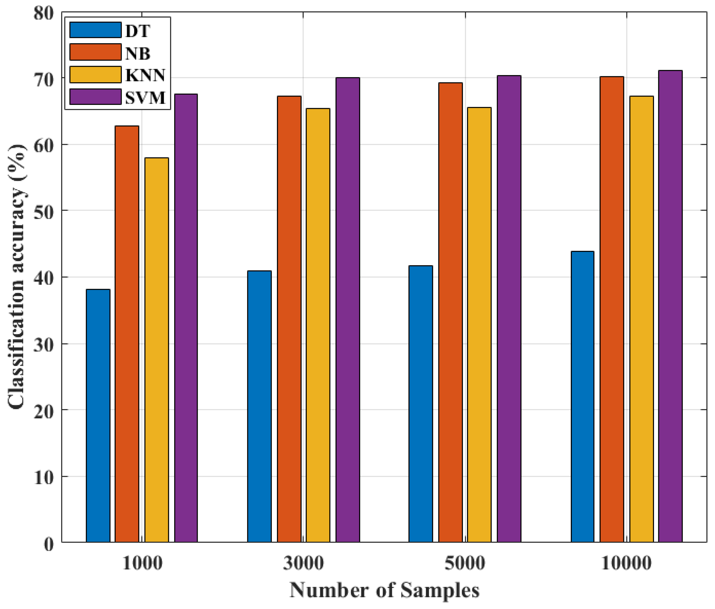
From Figure 4, it is observed that with an increased dataset size, ML models show an improvement in classification accuracy. Since the accuracy of classification does not improve any further after 10,000 samples, all models are trained for the same number of samples.

Table 6. Comparing the classification accuracy vs. dataset size for several ML algorithms.

Number of Samples	Achieved Percentage of Accuracy
	DT	NB	KNN	SVM
1000	38.2%	62.8%	57.9%	67.6%
3000	40.9%	67.2%	65.3%	70%
5000	41.7%	69.2%	65.6%	70.3%
10,000	43.8%	70.2%	67.2%	71.1%

compares the classification accuracies of several ML algorithms with different sample counts. SVM has the highest accuracy in classification (71.1%), NB has the second greatest accuracy (70.2%), followed by KNN (67.2%), and DT has the lowest classification accuracy (43.8%).

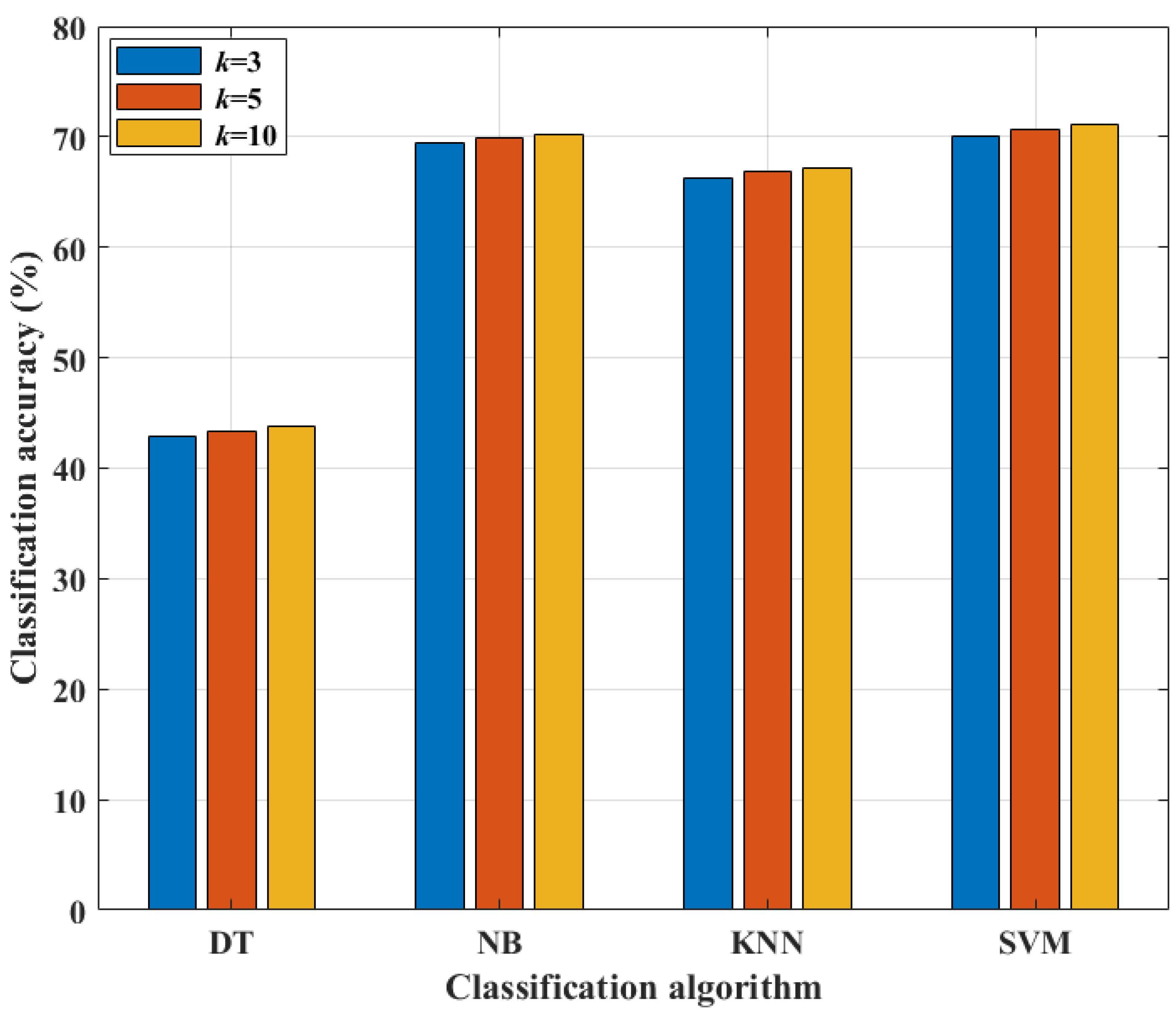
Cross-validation is an approach that allows the model to learn from many train–test splits. This provides a better idea of how well the trained model will perform on data that have not been seen before. In contrast, hold-out is based on a single train–test split. As a result, the hold-out method’s score is influenced by the way the data are divided into train and test sets. Figure 5 and

Table 7. Comparing the distinct TAS techniques based on their accuracy performances.

ML-Based TAS Scheme	Achieved Percentage of Accuracy
	$\mathit{k}$ = 3	$\mathit{k}$ = 5	$\mathit{k}$ = 10
SVM-based TAS [22]	70.1%	70.7%	71.1%
NB-based TAS [21,27]	69.5%	69.9%	70.2%
DT-based TAS [21,28]	42.9%	43.3%	43.8%
KNN-based TAS [22]	66.2%	66.8%	67.2%

show how altering the value of k-folds during cross-validation improves classification accuracy. The highest classification accuracy is observed for k = 10. As a result, the value of k is set to 10.

After performing normalization, these models are trained for four distinct features, as discussed earlier in Section 3.3. The complexities of all features based on their attribute vector lengths are listed in

Table 8. Complexity associated with different features based on the feature vector length.

Selected Feature	Length of the Feature Vector $\left({\mathit{N}}_{\mathit{Q}}\right)$	Configuration 1 $({\mathit{N}}_{\mathbf{rx}}=2,{\mathit{N}}_{\mathit{T}}=6)$	Configuration 2 $({\mathit{N}}_{\mathbf{rx}}=4,{\mathit{N}}_{\mathit{T}}=10)$
$\left|{\mathit{h}}_{i,j}^n\right|$	$N_{rx}\times N_T$	12	40
$\measuredangle \left(h_{i,j}^n\right)$	$N_{rx}\times N_T$	12	40
${\left|{\mathit{h}}_{i,j}^n\right|}^2$	$N_{rx}\times N_T$	12	40
${\left|{{\mathit{h}}_{i,j}^n}^H{\mathit{h}}_{i,j}^n\right|}^2$	$N_T\times N_T$	36	100

. The worst-performing attribute is $\measuredangle \left(h_{i,j}^n\right)$. Attribute 4 performs well only for DT, but its complexity increases with a higher-order configuration, so it is discarded. Combining features lengthens the feature vector and increases model complexity; hence, feature combination is avoided in this study. The absolute feature outperforms the other features in SVM, NB, and KNN, and its complexity is low; thus, only the absolute feature is utilized for this work.

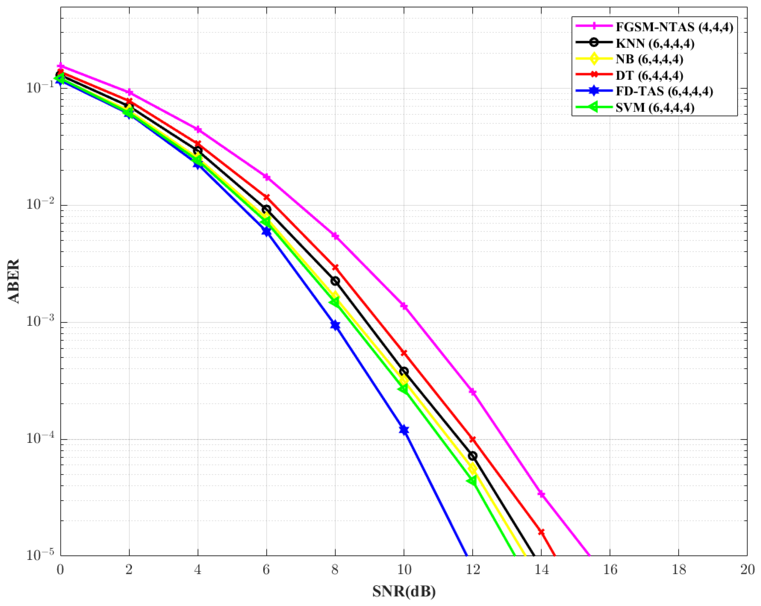
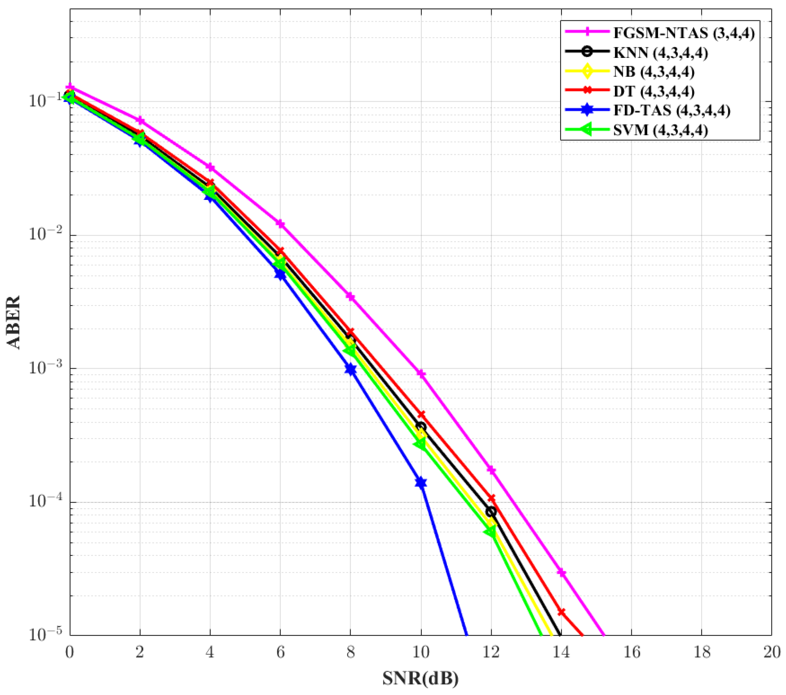
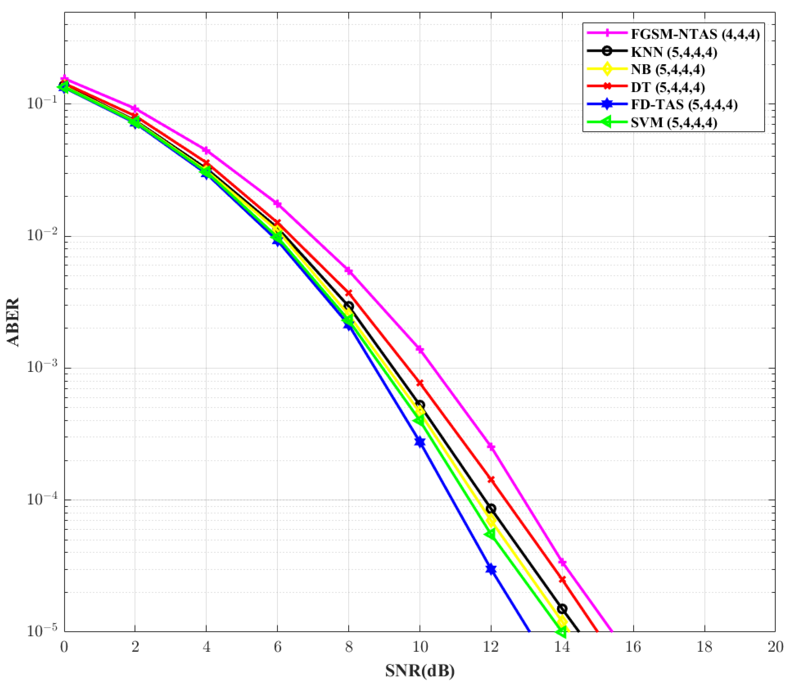
After conventional FD-TAS, the SVM-based TAS scheme outshines other ML-based systems, as shown in Figure 6. In comparison to the FGSM-NTAS method, the SVM-based TAS scheme cut downs the SNR need by ∼2 dB. This analysis is conducted for $N_T$ = 4, $N_{tx}$ = 3, $N_{rx}$ = 4, and M = 4. The ABER performance of the system is re-examined in Figure 7 by increasing the constellation order to 16. 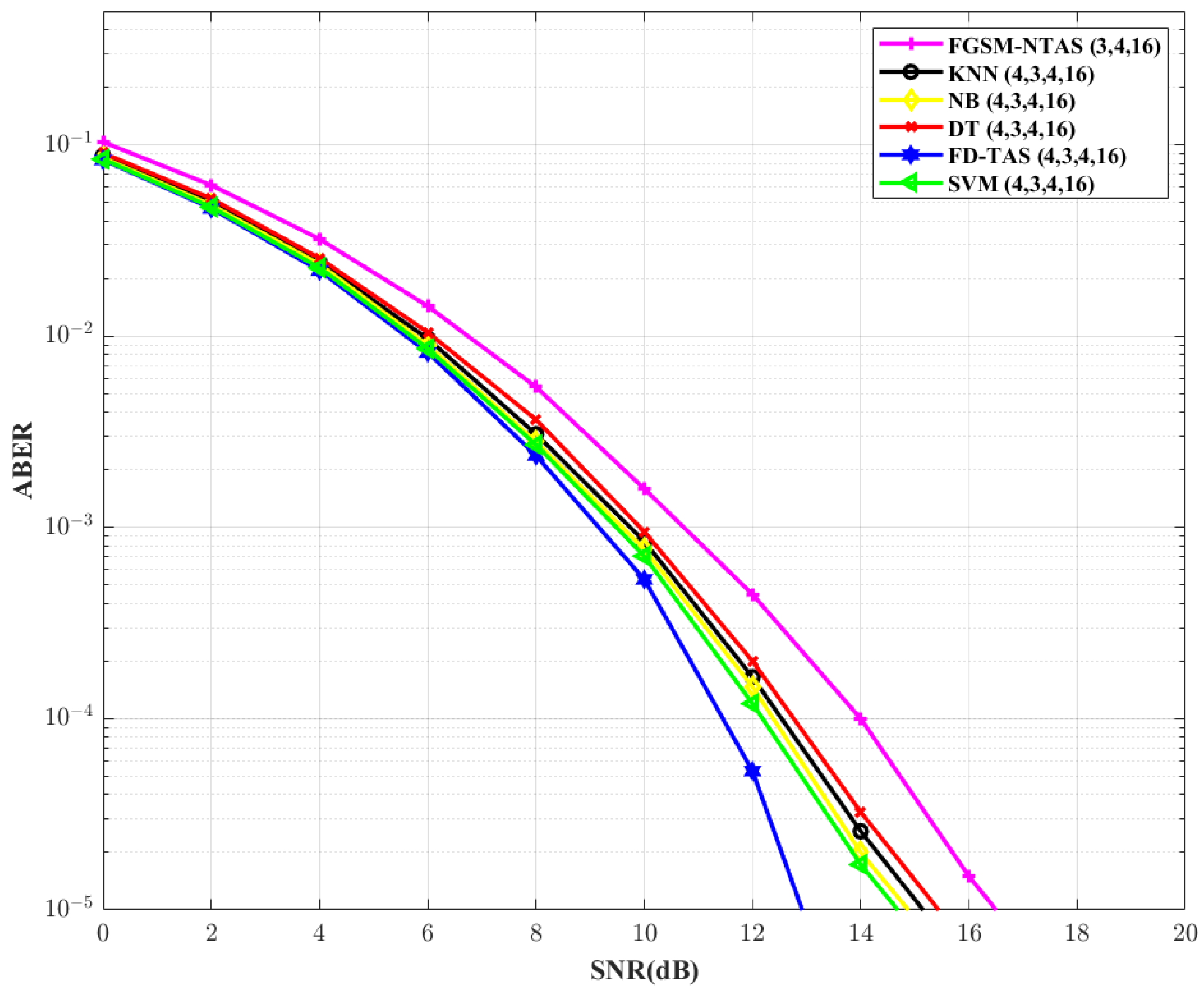For larger values of M, the SNR requirement for all ML-based methods increases. For FGSM-NTAS and conventional FD-TAS SNR gain requirements increase by ∼1.3 dB and ∼1.61 dB, respectively. SVM outperforms the FGSM-NTAS system in this circumstance as well, with a gain improvement of ∼2 dB.

Figure 8 analyzes the ABERs of different TAS schemes for $N_T$ = 5, $N_{tx}$ = 4, $N_{rx}$ = 4, and M = 4 configuration. It is found that SVM-based TAS outperforms FGSM-NTAS by ∼1.42 dB in terms of SNR gain. By increasing $N_T$ to 6, the analysis is repeated in Figure 9. For traditional FD-TAS, the required SNR drops by ∼1.28 dB. For SVM, NB, KNN, and DT-based TAS systems, respectively, there is a reduction of ∼0.78 dB, ∼0.66 dB, ∼0.68 dB, and ∼0.59 dB in the SNR requirements. In comparison to the FGSM-NTAS system, the SVM-based TAS technique gains ∼2.2 dB.

Table 9. SNR gain achieved by distinct TAS practices over FGSM-NTAS.

ML-Based TAS Scheme	Improvement in SNR gain (dB)
	Configuration 1 (${\mathit{N}}_{\mathit{T}}$ = 4, ${\mathit{N}}_{\mathit{tx}}$ = 3, ${\mathit{N}}_{\mathit{rx}}$ = 4, and $\mathit{M}$ = 4)	Configuration 2 (${\mathit{N}}_{\mathit{T}}$ = 4, ${\mathit{N}}_{\mathit{tx}}$ = 3, ${\mathit{N}}_{\mathit{rx}}$ = 4, and $\mathit{M}$ = 16)	Configuration 3 (${\mathit{N}}_{\mathit{T}}$ = 5, ${\mathit{N}}_{\mathit{tx}}$ = 4, ${\mathit{N}}_{\mathit{rx}}$ = 4, and $\mathit{M}$ = 4)	Configuration 4 (${\mathit{N}}_{\mathit{T}}$ = 6, ${\mathit{N}}_{\mathit{tx}}$ = 4, ${\mathit{N}}_{\mathit{rx}}$ = 4, and $\mathit{M}$ = 4)
SVM-based TAS [22]	1.76	1.89	1.44	2.2
NB-based TAS [21,27]	1.49	1.65	1.21	1.86
DT-based TAS [21,28]	0.59	1.08	0.46	1.03
KNN-based TAS [22]	1.27	1.39	0.96	1.61

lists the SNR gain achieved by the proposed ML-based TAS practices over traditional FGSM-NTAS.

6. Conclusions

Four distinct ML-based TAS techniques are suggested and implemented for a small-scale MIMO-based FGSM system in this work. For different values of $N_T$, $N_{tx}$, and M, the recommended algorithm’s ABER performance is compared to those of FD-TAS and FGSM-NTAS. The SVM-based TAS scheme surpasses all proposed ML-based TAS approaches in the simulations. The ABER performance of SVM is poorer than FD-TAS but the SVM-based TAS scheme is more computationally efficient than FD-TAS. SVM-based TAS attains the highest classification accuracy (∼71.1%) and a minimal SNR gain of ∼2.2 dB compared to FGSM-NTAS. As a result, it may be a viable option for future-generation networks. These schemes, as well as DL-based architectures, can be implemented in the future for advanced SM variants. The proposed TAS strategies could be extended to massive MIMO systems.