Secure Partitioning of Cloud Applications, with Cost Look-Ahead

Abstract

The security of Cloud applications is a major concern for application developers and operators. Protecting users’ data confidentiality requires methods to avoid leakage from vulnerable software and unreliable Cloud providers. Recently, trusted execution environments (TEEs) emerged in Cloud settings to isolate applications from the privileged access of Cloud providers. Such hardware-based technologies exploit separation kernels, which aim at safely isolating the software components of applications. In this article, we propose a methodology to determine safe partitionings of Cloud applications to be deployed on TEEs. Through a probabilistic cost model, we enable application operators to select the best trade-off partitioning in terms of future re-partitioning costs and the number of domains. To the best of our knowledge, no previous proposal exists addressing such a problem. We exploit information-flow security techniques to protect the data confidentiality of applications by relying on declarative methods to model applications and their data flow. The proposed solution is assessed by executing a proof-of-concept implementation that shows the relationship among the future partitioning costs, number of domains and execution times.

1. Introduction

Cloud computing has grown considerably in the last few decades to support applications by remotely providing computation, storage and networking resources [1]. Nowadays, Cloud technologies are extensively adopted but open problems and issues still remain. Among them, the security aspects of Cloud computing represent a major concern of both fundamental research and development [2,3].

There are several lines of research in Cloud computing security [4], spanning from network layers [5] to virtualisation and multi-tenancy [6], from the software stack to specialised hardware [7], and from regulations to responsibility models [8]. A major concern about adopting the Cloud relates to the difficulty of guaranteeing the data confidentiality and code integrity of applications running on Cloud resources.

Most modern applications consist of large codebases that rely on third-party software, subject to regular updates and short development time. Such complexity makes it difficult to verify or certify the security assurances of the deployed software, also exposing applications to bugs that lead to exploitable vulnerabilities. Moreover, application operators manage, run and maintain the software relying on Cloud providers. Those providers deliver hardware and software infrastructure capabilities, maintaining high privileges on the access to the infrastructure [9]. From the data security point of view, Cloud infrastructure providers cannot be considered fully reliable, e.g., a malicious insider could abuse her access rights to steal secret data [10].

Consider a public Cloud scenario, where providers deliver hardware and software infrastructure to their customers managing applications made from software components (e.g., microservice architectures) and hardware components (e.g., network devices). Each software component of an application has a set of security-relevant characteristics, properties or software dependencies of the component, e.g., the use of a non-verified third-party library. Those characteristics determine the degree of trust of a component in order to establish whether the component can manage its data without leaks.

The usage of software with a low degree of trust can pave the way for attacks that compromise the confidentiality of applications’ data. Hence, application developers need mechanisms to: (i) identify how reliable software manages sensitive data, (ii) securely isolate components in order to avoid data leaks from unreliable software and (iii) be protected from unreliable infrastructure providers. To fulfil these requirements and protect the application data from the deployment phase onwards, developers can leverage dedicated hardware to separate the application components into isolated environments. This approach enables data flow solely through explicit communication channels and eludes the privileges of the hardware platform providers.

The most common technologies to provide this kind of isolation are separation kernels (SK). They create a computational environment indistinguishable from a distributed system, where information can only flow from one isolated machine to another through explicit communication channels [11]. In a nutshell, SKs are (hardware or software) mechanisms that partition the available resources in isolated domains (or partitions), mediate the information flow between them and protect all the resources from unauthorised accesses.

In Cloud settings, the hardware is not directly available to customers and trusted execution environments (TEEs) [12,13,14] are emerging to exploit the SK technology. TEEs are tamper-resistant processing environments that run on a separation kernel [15]. They allow customers to create isolated memory domains for code and data that are also not accessible by the privileged software that is controlled by Cloud providers. TEEs provide in the Cloud the same memory and register isolation that separation kernel (SK) technologies provide in local machines.

In this work, we focus on the data separation provided by SKs. We do not consider other sophisticated mechanisms offered, such as the timed scheduling of domains. Given that our discussion is not dependent on the hardware that isolates the domains, in the rest of our article we refer to SKs as the supporting technology that comprehends TEEs and other similar mechanisms.

To effectively adopt these technologies, developers must face several design choices. Deciding which components must be grouped together is particularly important and challenging. Developers must solve the problem of how to partition their applications, i.e., how to separate the software components of the application to be placed in different SKs’ domains. Our ultimate objective is to avoid potential data leaks after the deployment phase by exploiting applications’ information flow. Indeed, there is a research gap in addressing this problem. There exist information-flow security methods to address complementary problems, such as checking the correct labelling of software or monitoring the inputs and storage accesses by the applications. Other proposals rely on specialised hardware to tackle unreliable Cloud providers. As far as we know, however, there is no work that employs both aspects (viz., information-flow security and SK protection mechanisms in the Cloud) aiming at supporting the deployment of Cloud applications on specialised hardware such as SKs.

In our previous work [16], we presented a methodology to determine a (minimal) eligible partitioning of an application onto an SK. Namely, [16] presents:

(a) 

a declarative model to represent multi-component applications, exploiting information-flow security to check whether components can manage their data without leaks, and

(b) 

a (formal) definition of safely partitionable applications and eligible partitioning, also considering the performance cost of exploiting SKs and the cost of migrating software, prototyped in SKnife (Open-sourced at: https://github.com/di-unipi-socc/sk, accessed on 20 June 2023).

In this article, we extend (a) and (b), with the following original contributions:

(c) 

the sketch of the proof that the partitioning determined by SKnife is minimal and unique,

(d) 

a cost model based on the probability of deployment migration, which depends on user-defined parameters, viz., the upper limit of SK domains and the number of admitted changes in data secrecy and components’ trust,

(e) 

a novel (Prolog and Python) prototype, ProbSKnife (open-sourced at: https://github.com/di-unipi-socc/ProbSKnife, accessed on 20 June 2023), that exploits SKnife to determine the eligible partitionings and implements the above probabilistic cost model to support the decision-making related to the initial deployment of the application, and

(f) 

the experimental assessment of ProbSKnife considering the execution times, future costs and probability of not finding a safely partitionable application at varying input parameters.

The goal of our methodology is to support the decision-making of application operators for the deployment of their applications in Cloud settings where the infrastructure provider is considered not trusted, by exploiting the SK technology. Our prototype tool is able to determine the deployment using the minimum number of domains, e.g., with the lowest SK performance impact, or to recommend different solutions considering the trade-off between the number of domains and costs of future re-deployments.

The rest of this article is organised as follows. Section 2 deeply analyses the related literature. Section 3 introduces essential notions to prepare the ground for our methodology and a realistic motivating example. Section 4 describes our declarative modelling of multi-component applications and information-flow methods. Section 5 presents our partitioning methodology aiming at minimising the number of SK domains, prototyped in the Prolog open-source tool SKnife. Section 6 introduces the cost model of a deployment migration and the Prolog implementation ProbSKnife. Section 7 shows the results of the experimental assessment of ProbSKnife aiming at investigating the performance and future costs of the motivating example. Finally, Section 8 concludes the article by pointing to some lines for future work.

2. Related Work

2.1. Specialised Hardware for Cloud Security

The adoption of specialised hardware for security in Cloud scenarios is largely diffused [17,18,19,20,21] to address the issue to entrust applications and their data to Cloud providers. The two main technologies adopted are TEEs and enclaves, which share the idea to reserve a separate and protected region of memory for executing code that is not accessible or temperable by the owner of the machine by enabling secure data processing.

Zheng et al. [22] survey the literature that exploits enclave-based hardware and TEEs to build secure applications in the Cloud and possible attacks on such applications. Moreover, the authors highlight the overheads brought by those technologies in terms of memory usage, data and code encryption and the limited computing resources of the secure area. Relatedly, Zhao et al. [23] conduct an experimental study to evaluate enclave technology’s impact on application performance, measuring the overhead on function and system calls, memory accesses and data exchanged from and to the enclave. The authors conclude that such specialised hardware surely enhances the security of Cloud applications but it is very important to take care of the performance overhead. Arfaoui et al. [24] deeply analyse TEEs by comparing the currently available solutions, focusing on the security aspects.

2.2. Partitioning and Separation

Lind et al. [25] propose a framework to automatically partition C applications for deployment on enclaves to protect data confidentiality from an untrusted operating system. Differently from our work, they do not employ information-flow techniques to determine the partitioning but rely on annotations of the source code as an indication of what should be placed in the enclave. Without considering specialised hardware, other works perform least-privilege application partitioning on source code relying on static analysis [26,27], dynamic analysis [28,29] or their combination [30].

In Cloud settings, Watson et al. [31] propose a methodology to support the deployment of applications composed of service workflows that are partitioned on Cloud nodes based on the security requirements of the data flow. Other approaches aim at verifying the data separation and the data flow of SKs [32,33,34,35]. In mobile settings, Rubinov et al. [36] propose a partitioning framework for placing Android applications on TEEs. By mixing source code annotations and taint analysis, the framework indicates to the user a refactoring of the application in order to isolate the most sensitive parts. Differently from our work, this framework needs to analyse the source code and it is language-specific and OS-specific.

2.3. Information-Flow Security

Information-flow security assigns labels to variables of a program to follow its data flow in order to verify the desired properties (e.g., non-interference [37]) and avoids covert channels. Labels are ordered in a security lattice to represent the relations of the labels from the highest ones (e.g., top secret) to the lowest ones (e.g., public data). Security lattices can be arbitrarily complex and define total or partial orders, e.g., a three-label total order that represents data secrecy from top secret to low secret is represented as top ≻ medium ≻ low.

Some approaches use information-flow security to address problems that are complementary to our techniques, for example, checking the correct labelling of software or monitoring inputs and storage accesses by the applications. Elsayed and Zulkernine [38] propose a framework to deliver Information-Flow-Control-as-a-Service (IFCaaS) in order to protect the confidentiality and integrity of the information flow in a Software-as-a-Service application. The framework works as a trusted party that creates a call graph of an application from the source code and applies information-flow security based on dependence graphs to detect violations of the non-interference policy.

At the Function-as-a-Service (FaaS) level, Alpernas et al. [39] present an approach for dynamic information-flow control, monitoring the inputs of serverless functions to tag them with suitable security labels in order to check access to data storage and communication channels to prevent leaks of the data managed by the functions. Similarly, Datta et al. [40] propose to monitor serverless functions by starting to learn the information flow of an application, showing the detected flows to the developers and enforcing the selected ones.

In the Cloud–Edge continuum, our previous work [41] exploits information-flow security to place FaaS orchestrations on Fog infrastructures. Functions are labelled with security types according to the input received and infrastructure nodes are labelled according to user-defined security policies. The placements are considered eligible if every node involved has a security type greater than or equal to the security type of all the hosted serverless functions. Developers assign a level of trust to infrastructure providers that concurs to rank the eligible placements.

Differently from our approach, all these proposals but [38] consider Cloud–Edge providers reliable. Recently, a few proposals have leveraged information-flow analyses to enforce data security in Cloud applications when the Cloud–Edge provider is untrusted. For example, Oak et al. [42] have extended Java with information-flow annotations that allow verification of whether partitioning an application into components that run inside and outside an SGX enclave violates confidentiality security policies. In this proposal, partitioning is decided by the programmer.

2.4. Declarative Approaches

Similarly to us, declarative techniques have been employed to resolve different Cloud-related problems. There are proposals to manage Cloud resources (e.g., [43]), to improve network usage (e.g., [44]), to assess the security and trust levels of different application placements (e.g., [45]) and to securely place VNF chains and steer traffic across them (e.g., [46]).

To the best of our knowledge, there are currently no proposals that employ information-flow security to partition applications to support the deployment on SKs.

3. Preliminaries

3.1. Threat Model

Table 1. Threat model.

Asset	Data confidentiality
TCBs	Application operator, TEE/SK
Threat	Cloud Provider	External Attacker
Attack Vectors	Superuser Privileges	Software Vulnerabilities, Covert Channels
Countermeasures	TEE, SK	Eligible Partitioning

shows the threat model considered hereinafter. Our goal is to protect the data confidentiality of multi-component Cloud applications from external attackers and unreliable Cloud providers.

Application developers are assumed to be trusted, and the information they give about the application to protect is considered reliable. Our trusted computing base (TCB) leverages the SK technology to isolate the software components of an application into separate domains, guaranteeing that the information flows only along the explicit communication lines given by the application developers and avoiding other side channels. This model is consistent with the threat model of several trusted execution environments (e.g., [47]).

Software components can be hacked by external attackers by exploiting their vulnerabilities to leak application data. As an example, an attacker can gain control of a software component from a malicious or bugged library and steal the data managed by that component itself or by the components in the same environment, i.e., domain.

Moreover, a component under the control of an attacker can create covert channels, e.g., by sending stolen data via the network. For these reasons, we need to take particular care in individuating less-trusted components and isolating them from components managing important data. Exploiting SKs guarantees that communication only happens through explicit channels, avoiding the creation of side channels. However, we need to pay particular attention to software components having explicit channels toward the hardware that can be exploited by compromised software components, i.e., creating a path to leak the data.

On the other hand, unreliable infrastructure providers can exploit their superuser privileges on the infrastructure to steal application data. We exploit TEEs to protect the software components that guarantee a tamper-resistant processing environment and remote attestation that proves its trustworthiness for third parties [15]. What is not protected by TEEs is the data exchange with unreliable hardware components, such as network interfaces or storage disks. As an example, having an explicit channel to save secret data on a disk is admitted by TEEs independently from the partitioning of the software components and such data are leaked to the provider as the owner of the disk. Therefore, we need to take care of the secrecy of the data exchanged with hardware components considered not trusted.

3.2. Problem Formulation

We define a partitioning as the structuring of the software components of an application in non-empty parts called domains. Intuitively, a partitioning domain represents an isolated environment where data can flow (inbound or outbound) only by explicit communication channels. Inside every domain, data can potentially be shared.

Domains must satisfy the following two properties:

• data consistency, meaning that the software components of the same domain manage data with the same secrecy level, and
• reliability, meaning that the components of the same domain have the same trust from the operator to manage their data.

A partitioning is safe if and only if each of its domains is data-consistent and reliable.

An application is safely partitionable if it does not leak sensitive data from software components to untrusted hardware components. When an application is non-safely partitionable, exploiting the SK isolation is not enough to protect the data confidentiality of the application. Our approach detects this situation and suggests how to improve the software reliability or the data-secrecy level to make the application safely partitionable.

Overall, the problem addressed by this work can be stated as follows:

“Given a multi-component application consisting of a set S of software components, find safe partitionings of S (if any) in order to deploy the application A to an SK technology while minimising the considered costs and protecting A from data leaks.”

While tackling this problem, two main challenges are addressed. On one hand, the data confidentiality of applications must be considered during the deployment phase. On the other, the performance of applications should not be degraded by the supporting hardware technology that enforces security. We tackle the partitioning problem by employing information-flow security techniques [48]: (i) to understand whether the software components leak sensitive data outside the SK and (ii) to partition the application in order to avoid data leaks between components hosted on the same SK domain.

Moreover, to meet the security requirements it is enough to find a partitioning that isolates unreliable software components of the application in different domains, but doing so blindly can lead to unexpected performance and deployment costs. SKs bring overheads that can heavily impact the application performance [34], e.g., switching domains during the execution has a cost in terms of time that is influenced by sanitising the used resources before re-using them and by the domain-scheduling algorithm of the SK. Moreover, changing software domains after deployment requires working on the explicit communication channels that become intra-domain from extra-domain and vice versa. All of these call for partitionings that allow application operators to reduce those kinds of costs.

We consider two different cost parameters to determine safe partitioning:

• the number of domains used by the safe partitioning in order to reduce the SK overhead, and
• the expected migration cost of switching from one partitioning to another following new evidence about the software components in our application (e.g., disclosure of a new bug or defect bringing a vulnerability).

We also consider the combination of the above costs to support application operators in determining the best trade-off in terms of SK overhead and potential migration cost.

We propose two declarative methodologies and open-source prototypes:

• SKnife, which finds the minimal safe partitioning (Section 4) that minimises the number of domains, and
• ProbSKnife (Section 6.2), which exploits SKnife to find all the safe partitionings with their expected migration cost, up to a user-defined limit of the number of domains.

The first methodology, prototyped in SKnife, exploits logic programming to define partitionings and domains in such a way that they satisfy the data-consistency and -reliability properties. By applying inference rules to the application model, our Prolog prototype determines a minimal partitioning.

The second methodology, prototyped in ProbSKnife, determines all the possible initial partitionings (not only the minimal one) and computes the cost of changing deployment based on probability distributions that describe changes in the data classification and component trustability.

3.3. Motivating Example

Consider a Cloud-centralised IoT system that collects data sampled by sensors and sends them to a Cloud application, where the data are stored and used to decide which commands to issue to IoT actuators. The users of this application can make requests on the status of the devices and can remotely configure the application. Nowadays, these kinds of applications are well-established in the home-automation field [49], service-device compositions [50] and platforms offered by Cloud providers [51,52].

The architecture of the example application is depicted in Figure 1. Consider six software components and two hardware components—depicted in grey—that are used by the application, connected by edges representing explicit communication links between components.

Users and IoT devices perform REST invocations toward the considered application. All inbound communication passes through the Network Interface and is received by the API Gateway. The intra-application communication is performed by message passing between components, exploiting explicit channels supplied by the underlying hardware. The Authenticator decrypts and authenticates the inbound data and forwards them to the intended recipient.

Application users can send General requests and Configuration requests. The former are requests for explicit actuation or data previously sampled and are delivered to the App Manager, which is the main component of the application that implements the business logic. The latter are requests for reading or updating the current application configuration and are delivered to the User Configuration component, which manages the configuration of the application. The IoT devices send either sampled data or events, which are dispatched to the App Manager component. The outbound communication consists of responses to the users based on their requests or IoT commands from the App Manager toward the IoT devices. To store relevant application data—IoT Measurement and User Preferences—the application relies on the component DB, a database that is the only one connected to the Disk. Finally, AI Learning is a machine-learning module that uses IoT Measurement and User Preferences to perform predictions and support the decision-making of the App Manager.

Each component has explicit links to other components, its own data—depicted in the lower boxes of the components—and its relevant characteristics—depicted in the upper boxes of the components. For instance, the component AI Learning has data IoT Measurement and User Preference, its relevant characteristic is AI Framework and it is linked to App Manager and User Configuration. The characteristics are properties, third-party libraries, etc., that impact the trust of the components. For instance, the Disk is owned by the Cloud provider, which in our setting makes the component unreliable. The measure of the trust level of the components is mandatory to determine if they can manage their data in order to avoid leaks. For instance, the API Gateway must be able to manage its data to avoid the leak of such data toward the Network interface. The dotted arrow between User Config and Disk represents a link consisting of an alteration of the application architecture. Figure 1 represents two different application architectures with only that link as a difference. The base application—identified as iotApp1—does not have the dotted link. The modified application—identified as iotApp2—has the dotted link. We will use those two slightly different architectures in Section 5.4 when discussing the partitioning of the two applications.

This application results in a large codebase that includes the operating system, communication stacks, AI frameworks, etc, and also requires frequent updates. These factors make it hard to verify or certify the security of the released software. To determine the level of trust of the software components, we assign security labels to the relevant characteristics of the application. We also assign security labels to the application data in order to establish a direct relationship between the data and the trust of the software components. We adopt a total ordering security lattice (viz., top ≻ medium ≻ low) modelling the labels pertaining to both sensitive data and trusted characteristics. The top label denotes both secret data and high-trust characteristics, the medium label denotes both medium-secret data and medium-trust characteristics and the low label denotes public data and non-reliable characteristics.

A component having characteristics considered unreliable by the application developer is not able to manage secret data. This could cause a leak of its data toward the directly connected components or toward the software components hosted in the same isolation environment, i.e., container, virtual machine or SK domain. For instance, if the DBMS used by DB is not reliable—either because it is malicious or because it has vulnerabilities—the data of DB can leak toward the Disk, component owned by the Cloud Provider. Furthermore, if DB is isolated in the same SK domain of API Gateway (assuming an unreliable Net Library), the leak of data could flow from the DB to the Network Interface through the API Gateway.

We emphasise again that we aim at protecting the data confidentiality of applications placed on the Cloud by finding safe partitionings, i.e., grouping the software components in non-empty subsets that allow placement of the application in SK domains in such a way that the data and trust of the components are homogeneous in every domain, avoiding having less-trusted components share the environment with components that manage sensitive data. For instance, we already discussed that AI Framework is a library of AI Learning considered not reliable; it may contain malicious code or its vulnerabilities may be exploited by an external attacker. Placing all the software components in the same domain exposes the data of the application to be read by AI Framework and sent outside such domain. Partitioning the application components to isolate their data and exploiting the SKs’ isolation mitigates those kinds of threats.

To support the application operator’s decision, we aim at determining the expected migration costs of the software components. Migrating the software components could be needed after the deployment of the partitioned applications due to events such as bug discovery or data declassification that bring a change in the labelling of the application. With the new labelling, the partitioning might not be safe anymore. For instance, a bug discovered in the TLS Library declassifies its trust from top to medium and the Authenticator must be migrated to a different domain to preserve the data confidentiality of the application.

For these reasons, every software component is also annotated with its migration cost, represented as an integer number. The migration cost represents how many hours of work are needed to change the communication link of each software component during a migration that changes the status of the link from intra-domain to extra-domain and vice versa. For instance, the User Configuration needs 10 person hours to change its communication links.

To evaluate the expected costs of migration, we need to know how data and characteristics can change the label over time. Application operators may determine the probability distribution of the change over time by their experience or by exploiting statistical analyses from the open-source community [53].

Table 2. Probability distributions to change the label for each data type and characteristic.

DATA/CHARACTER	PROBABILITY (%)
	Top	Medium	Low
Network Data	0	0	100
Crypted Data	0	0	100
User Preferences	30	50	20
User Requests	30	50	20
IoT Measurements	70	20	10
IoT Events	70	20	10
IoT Commands	80	10	10
TLS Library	70	20	10
From Provider	10	30	60
AI Framework	20	30	50
DBMS	50	30	20
Net. Library	10	20	70
Data Library	30	40	30

shows a probability distribution to change the label for each data and characteristic of the application.

For instance, we can assume that in the future there is a $20\%$ probability of discovering a side channel not easy to exploit in the TLS Library, reducing its trust from top to medium. Alternatively, there is a $10\%$ probability of discovering a vulnerability in the cryptography algorithm of the same library, which reduces its trust to low. We represent this by assigning to the TLS Library $20\%$ as the probability of changing its label to medium, $10\%$ as the probability of changing its label to low and s $70\%$ as the probability of remaining top.

From Table 2, we can also deduce that the application operator does not exclude the possibility to consider reliable the Cloud provider in the future. Indeed, the From Provider characteristic has a $30\%$ probability of changing to medium trust and a $10\%$ probability of changing to top trust. Network Data and Crypted Data will be always considered low data as they have a $100\%$ probability of remaining low. This means that the application operator assumes that the data arriving from the network and the data stored on the Disk will never be secret.

4. A Declarative Solution: SKnife

This section describes the methodology implemented in SKnife to determine the minimal safe partitioning of an application for the deployment onto an SK by exploiting simple examples excerpted from the motivating example of Section 3.3. The model code (Section 4.1) is presented and discussed inline within the main text. The declarative implementation of our methodology (Section 4.2 and Section 5) is instead presented through code listings featuring line numbers to facilitate a more thorough discussion.

Werecall that a Prolog program is a finite set of clauses of the form a :- b1, …, bn stating that a holds when b1 $\wedge \cdots \wedge$ bn holds, where n ≥ 0 and a, b1, …, bn are atomic literals. Clauses with an empty condition are also called facts. Prolog variables begin with upper-case letters, lists are denoted by square brackets and negation is by \+. With pname/n is indicated a predicate with name pname and its arity n. Prolog programs can be queried, and the Prolog interpreter tries to answer each query by applying SLD resolution and by returning a computed answer substitution instantiating the variables in the query.

4.1. Declarative Modelling Applications and Labelling

Application developers model their applications through suitable Prolog facts and clauses, as

application(AppId,Hardware,Software).

where AppId is the application identifier, Hardware is the list of hardware components interacting with the application and Software is the list of software components to place on the SK.

Example. 

The iotApp1 application of our example is declared by the fact

application(iotApp1,[network,disk],[userConfig,appManager,

authenticator,aiLearning,apiGateway,db]).

Software and hardware components are declared as in

software(SwId,Data,Characts,Cost,[LinkedHW,LinkedSW]).

hardware(HwId,Data,Characts,[LinkedHW,LinkedSW]).

where SwId and HwId are the unique identifiers of each component, Data is the list of names of the data managed by the component, Characts is the list of names of the component characteristics, LinkedHW is the list of linked hardware components and LinkedSW is the list of linked software components. The only difference is the components definition Cost, which is the integer value representing the migration cost of the software.

Example. 

The db and disk components are declared as

software(db,[iotMeasurements,userPreferences,cryptedData],

[dbms],50,([disk],[userConfig,appManager])).

hardware(disk,[cryptedData],[fromProvider],([],[db])).

Application developers must also declare a security lattice formed by ordered labels and they have to label the relevant data of the application and the relevant characteristics of the components. The higher the label of the data, the higher the secrecy of the data. Similarly, the higher the label of a characteristic, the higher the trust in the characteristic. We call the labels assigned to the data secrecy labels and the labels assigned to the characteristics trust labels.

Every data type and characteristic can be labelled using

tag(Name, Label).

where Name is the name of the data or characteristic to be labelled and Label is the assigned label. Obviously, the labels must be part of the lattice. We call labelling the set of all pairs 〈Name,Label〉 where all data and characteristics have been assigned a security label.

Example. 

The label of the data and the characteristics of the Disk are declared as

tag(cryptedData, low).

tag(fromProvider, low).

which represents the cryptedData data with a low secrecy label and the fromProvider characteristic with a low trust label.

The probability of changing the label for a data type or characteristic is declared as

tagChange(DC,label,P).

representing how the data or characteristic DC changes to label with probability P. To have the full distribution for DC we need facts for every label of the security lattice and the sum of the probabilities of those facts must be 1.

Example. 

The probabilities of changing the label of the data and the characteristics of the Disk are declared as

tagChange(cryptedData,    top,    0.0).

tagChange(cryptedData,    medium, 0.0).

tagChange(cryptedData,    low,    1.0).

tagChange(fromProvider,    top,    0.1).

tagChange(fromProvider,    medium, 0.3).

tagChange(fromProvider,    low,    0.6).

which represents the cryptedData data with a probability of $100\%$ to have a low secrecy label and the fromProvider characteristic with a probability of $60\%$ to remain low, $30\%$ to change to medium and $30\%$ to change to top.

4.2. Safe Partitioning

Our methodology assigns to every component a pair of labels, one indicating its secrecy level and one indicating its trust level. A component is trusted if its trust label is greater than or equal to its secrecy label; otherwise, it is considered untrusted. All the comparisons between labels are based on the ordering of the security lattice. A trusted component is able to manage its data without the risk of leaking them.

The label assignment to a component is performed by the predicate labelC/4 of Listing 1, using the lists of data and characteristics of the component and the labelling of the application.

Listing 1. The labelC/4 predicate.

The secrecy label is determined by the highest label of its data in order to consider the most critical data managed by the component. The trust label is determined by the lowest label of its characteristics because the worst characteristic could compromise the trust of the component, e.g., a component using a simple logging library and a certified encryption software could be endangered by a bug in the former.

A component without relevant characteristics is considered reliable and its trust label is the highest of the security lattice. We choose this level of granularity (i.e., the developer labels the data and characteristics instead of directly labelling the components) to have a better insight into the application and to have a more accurate understanding of the situations in which the application is non-safely partitionable.

Untrusted components can leak their data to directly linked components. If such components have a trust label lower than the leaked data they can propagate the leakage through their links. If such data reach a hardware component, then an external leak occurs. An external leak is a path from an untrusted software component to a hardware component where all the components of the path have a trust label lower than the secrecy label of the first software component of the path. The presence of such paths indicates the potential for data leakage from an untrusted component toward the outside of the SK that is not avoidable by the partitioning.

Recall that an application is called safely partitionable when there is no leakage outside the SK, i.e., all its hardware components are trusted and all its untrusted software components do not incur any external leaks.

The predicate hardwareOk/2 of Listing 2 checks that all the hardware components of the application are trusted, which avoids hardware attacks that cannot be contrasted by the SK partitioning.

Listing 2. The hardwareOk/2 predicate.

The predicate recursively scans the list of hardware components to check their labelling. Initially, information about a single component is retrieved (line 7), and then the labelling of the hardware component is determined (line 8). The predicate checks for the component trustability (line 9), where gte/2 checks if the trust is greater than or equal to the secrecy. Finally, hardwareOk/2 recurs on the rest of the list (line 10) until it is empty (line 11).

Similarly, the predicate softwareOk/2 of Listing 3 checks that no software component (line 13) that is untrusted (line 14) has an external leak toward an untrusted hardware component (line 15).

Listing 3. The softwareOk/2 predicate.

5. Determining the Minimal Safe Partitioning

In this section, we first show how SKnife determines a minimal safe partitioning of an application onto an SK. We then also present a technique to support the application operator when the application is non-safely partitionable.

5.1. Minimal Number of Domains

As aforementioned, we initially consider the number of domains in a partitioning P as its cost, as shown in Equation (1), where $\left|P\right|$ indicates the cardinality of the partitioning:

$$Cost\left(P\right)=\left|P\right|$$

(1)

Solving the partitioning problem with such a cost corresponds to determining a safe partitioning $P_{min}$ with the minimum number of domains. Given an application a, a labelling $\mathcal{L}$ and a security lattice L,

$$\mathtt{SKnife}(a,\mathcal{L},L)=P_{min}$$

(2)

$$P_{min}=\underset{i}{\mathrm{argmin}}\left|P_i\right|$$

(3)

Such a partitioning is unique (see proof in Section 5.2) and its cost depends on the number of labels of the security lattices. Note that, the minimum number of domains needed to safely partition an application is equal to the number of label configurations to satisfy the data-consistency and reliability properties. By counting all possible configurations, an upper bound to the minimum number of domains is $\frac{L^2}{s}$. We will prove later how, by construction, SKnife determines the minimal safe partitioning.

5.2. Declarative Strategy for the Minimal Safe Partitioning

We use the notation $P\vDash \mathcal{L}$ to indicate that a partitioning P satisfies a labelling $\mathcal{L}$ when the partitioning is safe with $\mathcal{L}$.

Safe partitionings split safely partitionable applications into a set of data-consistent and reliable domains.

The software components of a safely partitionable application can be split and placed on SK domains. A domain is a triple (DTData, DTChar, HostedSw) where DTData is the secrecy label of the domain, DTChar is the trust label of the domain and HostedSw is the list of the software components hosted by the domain. Inside a domain, the software components share the same environment. To avoid placing components in an environment containing data that they are not able to manage, a domain must be data-consistent, as defined in Equation (4)

$$\begin{array}{c}\hfill \mathtt{\forall }\mathtt{software}\mathtt{(}\mathtt{Sw},\mathtt{Data},\mathtt{Characteristics}, \mathtt{\_}\mathtt{)}\mathtt{\in }\mathtt{H}\mathtt{o}\mathtt{s}\mathtt{t}\mathtt{e}\mathtt{d}\mathtt{S}\mathtt{w}:\\ \hfill \mathtt{l}\mathtt{a}\mathtt{b}\mathtt{e}\mathtt{l}\mathtt{C}\mathtt{(}\mathtt{D}\mathtt{a}\mathtt{t}\mathtt{a},\mathtt{C}\mathtt{h}\mathtt{a}\mathtt{r}\mathtt{a}\mathtt{c}\mathtt{t}\mathtt{e}\mathtt{r}\mathtt{i}\mathtt{s}\mathtt{t}\mathtt{i}\mathtt{c}\mathtt{s},\mathtt{(}\mathtt{C}\mathtt{T}\mathtt{D}\mathtt{a}\mathtt{t}\mathtt{a}, \mathtt{\_}\mathtt{\left)}\mathtt{\right)}\mathtt{\to }\mathtt{D}\mathtt{T}\mathtt{D}\mathtt{a}\mathtt{t}\mathtt{a}\mathtt{=}\mathtt{C}\mathtt{T}\mathtt{D}\mathtt{a}\mathtt{t}\mathtt{a}\end{array}$$

(4)

meaning that in a domain there is no software component with a secrecy label different from the domain secrecy label, i.e., all the software components hosted by a domain have the same secrecy label of the domain. This property avoids placing a software component in a domain that contains data more sensitive than those the component is supposed to deal with.

Another aspect to consider is that untrusted components bring out the risk of leaking sensitive data to other components of the domain or to linked components outside the domain. In order to isolate such components, the domains must be reliable, as defined in Equation (5)

$$\begin{array}{c}\hfill \mathtt{\forall }\mathtt{s}\mathtt{o}\mathtt{f}\mathtt{t}\mathtt{w}\mathtt{a}\mathtt{r}\mathtt{e}\mathtt{(}\mathtt{S}\mathtt{w},\mathtt{D}\mathtt{a}\mathtt{t}\mathtt{a},\mathtt{C}\mathtt{h}\mathtt{a}\mathtt{r}\mathtt{a}\mathtt{c}\mathtt{t}\mathtt{e}\mathtt{r}\mathtt{i}\mathtt{s}\mathtt{t}\mathtt{i}\mathtt{c}\mathtt{s},\_\mathtt{)}\mathtt{\in }\mathtt{H}\mathtt{o}\mathtt{s}\mathtt{t}\mathtt{e}\mathtt{d}\mathtt{S}\mathtt{w}\mathtt{:}\\ \hfill \mathtt{l}\mathtt{a}\mathtt{b}\mathtt{e}\mathtt{l}\mathtt{C}\mathtt{(}\mathtt{D}\mathtt{a}\mathtt{t}\mathtt{a},\mathtt{C}\mathtt{h}\mathtt{a}\mathtt{r}\mathtt{a}\mathtt{c}\mathtt{t}\mathtt{e}\mathtt{r}\mathtt{i}\mathtt{s}\mathtt{t}\mathtt{i}\mathtt{c}\mathtt{s},\mathtt{(}\mathtt{C}\mathtt{T}\mathtt{D}\mathtt{a}\mathtt{t}\mathtt{a},\mathtt{C}\mathtt{T}\mathtt{C}\mathtt{h}\mathtt{a}\mathtt{r}\mathtt{\left)}\mathtt{\right)}\mathtt{\to }\mathtt{C}\mathtt{T}\mathtt{D}\mathtt{a}\mathtt{t}\mathtt{a}\mathtt{\ge }\mathtt{C}\mathtt{T}\mathtt{C}\mathtt{h}\mathtt{a}\mathtt{r}\\ \hfill \mathtt{\vee }\\ \hfill \mathtt{\forall }\mathtt{s}\mathtt{o}\mathtt{f}\mathtt{t}\mathtt{w}\mathtt{a}\mathtt{r}\mathtt{e}\mathtt{(}\mathtt{S}\mathtt{w},\mathtt{D}\mathtt{a}\mathtt{t}\mathtt{a},\mathtt{C}\mathtt{h}\mathtt{a}\mathtt{r}\mathtt{a}\mathtt{c}\mathtt{t}\mathtt{e}\mathtt{r}\mathtt{i}\mathtt{s}\mathtt{t}\mathtt{i}\mathtt{c}\mathtt{s}, \mathtt{\_})\mathtt{\in }\mathtt{H}\mathtt{o}\mathtt{s}\mathtt{t}\mathtt{e}\mathtt{d}\mathtt{S}\mathtt{w}\mathtt{:}\\ \hfill \mathtt{l}\mathtt{a}\mathtt{b}\mathtt{e}\mathtt{l}\mathtt{C}\mathtt{(}\mathtt{D}\mathtt{a}\mathtt{t}\mathtt{a},\mathtt{C}\mathtt{h}\mathtt{a}\mathtt{r}\mathtt{a}\mathtt{c}\mathtt{t}\mathtt{e}\mathtt{r}\mathtt{i}\mathtt{s}\mathtt{t}\mathtt{i}\mathtt{c}\mathtt{s},\mathtt{(}\mathtt{C}\mathtt{T}\mathtt{D}\mathtt{a}\mathtt{t}\mathtt{a},\mathtt{C}\mathtt{T}\mathtt{C}\mathtt{h}\mathtt{a}\mathtt{r}\mathtt{\left)}\mathtt{\right)}\mathtt{\to }\mathtt{C}\mathtt{T}\mathtt{C}\mathtt{h}\mathtt{a}\mathtt{r}\mathtt{=}\mathtt{D}\mathtt{T}\mathtt{C}\mathtt{h}\mathtt{a}\mathtt{r}\end{array}$$

(5)

meaning that all the software components of a domain are either trusted or have the same trust label as the domain.

Domains hosting only trustable software components are considered secure from data leaks. Every component can manage its data and can exchange it outside the domain without the risk of leaks, according to the trust assigned by the developer. Untrusted components must be strongly isolated, and they can share a domain only with other untrusted components having the same trust label, in order to have a homogeneous level of trust inside the domain and mitigate the danger of a data leak.

The top-level sKnife/3 predicate (Listing 4) finds the safe partitioning of a safely partitionable application. After retrieving the application information (line 17), it performs two main steps. First, it checks whether the application is safely partitionable (lines 18–20) and then, it creates the set of data-consistent and reliable domains, splitting the software component across them (line 21), starting from an empty partitioning ([] of line 21).

Listing 4. The sKnife/3 predicate.

The partitioning/3 predicate is listed in Listing 5 and it has the task of splitting the labelled software components, placing them in data-consistent and reliable domains. The predicate recursively scans the list of labelled software components (LabelledSoftware) to place every component starting from a partitioning (Partitioning) that will be updated in the resulting partitioning (NewPartitioning). The domains of the resulting partitioning are data-consistent and reliable by construction. Every software component is placed in a domain with the same secrecy label to satisfy the data consistency of the domain.

Listing 5. The partitioning/3 predicate.

Trusted components are placed together in domains with the trust label named safe, indicating that all the hosted components are trusted. Untrusted components are placed in the domain with the same trust label, in order to create reliable domains. If the domain needed by a component is not in the starting partitioning, it is created with the correct labels and added to the partitioning.

partitioning/3 has two main clauses (lines 22 and 27) and the empty software list case that leaves the partitioning unmodified (line 32). The first case describes the situation in which a software element can be placed on a domain already created. After determining the labelling of the hosting domain (line 23), the library predicate select/3 checks if such a domain is already created in the partitioning (line 24) and extracts it. Then, an updated domain is created by adding the current software component (line 25). Finally, partitioning/3 recurs on the rest of the software list, giving as the starting partitioning the old partitioning with the updated domain ([DNew|TmpPartitioning] of line 26).

The second clause of the predicate (line 27) describes the situation in which the domain that has to host the software component is not already in the input partitioning. The initial step to determine the hosting-domain labelling is the same as the previous clause (line 28). Then, there is an explicit check that such a domain is not already in the partitioning (line 29). At this point, the new domain is created (line 30) and it is included in the partitioning during the recursive call ([DNew | Partitioning] of line 31).

Figure 2 sketches the steps followed by our methodology to determine the minimal partitioning.

As a safe partitioning example, the output of SKnife is represented by the four domains

• ((top,safe),[appManager,db,authernicator]),
• ((medium,safe),[userConfig]),
• ((low,safe),[apiGateway]),
• ((top,low),[aiLearning]).

where each domain is represented by their triple (DTData, DTChar, HostedSw), where DTData and DTChar are a pair of labels (or safe) and HostedSw is a list of software components.

In the following, we outline a proof to demonstrate that SKnife computes the minimal safe partitioning of the input application, if any.

Proof of Partitioning Minimality). 

As aforementioned, SKnife’s main predicate fails if the application is non-safely partitionable. This is checked by hardwareOk/2 of Listing 2 and softwareOk/2 of Listing 3. The minimum number of domains is not fixed for all possible applications, because it depends on the number of security types of the lattice and on the labelling of the application to be placed.

To prove that the result of SKnife is the minimal partitioning, it is enough to prove that the predicate partioning/3 of Listing 5 creates the minimal partitioning. We sketch the proof of minimality by defining the invariant of the partioning/3 predicate, which maintains the safety of the partitioning. Then, we show by induction that the invariant is preserved and that the resulting partitioning is minimal and unique.

A partitioning is a set of domains. We denote a domain as a triple $(d,c,sw)$ where d is the secrecy label given by data, c is the trust label given by characteristics and $sw$ is the list of software components hosted by the domain. The predicate partioning/3 implements a function

$$partitioning:S\times P\to P$$

where S is the software components set and P is the partitioning set.

We indicate with $\lambda$ the function that gives the labelling of a software component and $\varphi$ the function that gives the labelling of the domain needed by a software component. The function $partitioning$ has the following invariant:

$$\forall (d,safe,sw)\in P:\forall s\in sw\lambda \left(s\right)=(d,c)c\ge d\varphi \left(s\right)=(d,safe)$$

(6)

$$\forall (d,c,sw)\in P\wedge c\ne safe:\forall s\in sw\lambda \left(s\right)=(d,c)c\le d\varphi \left(s\right)=(d,c)$$

(7)

$$\forall (d,c,sw),(d^{\prime },c^{\prime },s{w}^{\prime })\in P:d=d^{\prime }\wedge c=c^{\prime }\Rightarrow sw=s{w}^{\prime }$$

(8)

$$\forall (d,c,sw)\in P:sw\ne \varnothing$$

(9)

Equations (6) and (7) indicate the labelling of software components and domains to satisfy the data-consistent and reliable-domain properties. Equation (8) indicates that no domains with the same labelling are admitted. Equation (9) indicates that empty domains do not exist.

We can prove by induction that the function $partitioning$ creates the minimal partitioning.

Base Case

$$partitioning\left(\right[],P)=P$$

an empty list of software components does not modify the partitioning.

Induction Step

$$P_i=partitioning([s{w}_i:sws],P_{i-1})$$

$$P_i=\left\{\begin{array}{c}{P}_{i-1}\backslash \left\{(d,c,sw)\right\}\cup \left\{(d,c,\{sw\cup s{w}_i\})\right\}\mathrm{if}\varphi \left(s{w}_i\right)=(d,c)\in P_{i-1}\hfill \\ \\ P_{i-1}\cup \left\{(d,c,\left\{s{w}_i\right\})\right\} \mathrm{otherwise}\hfill \end{array}\right.$$

We assume, by the inductive hypothesis, that the invariant holds up to the i-th step, i.e., for the domain of components [$s{w}_1$, …, $s{w}_i$]. It is easy to see that at step $(i+1)$ the current $s{w}_{i+1}$ is suitably placed into an existing domain (first clause of partitioning/3) or inserted into a new one (second clause of partitioning/3) by following the rule above. Assume that after this step, the invariant does not hold, i.e., that the resulting domain is non-minimal. Then, as $s{w}_{i+1}$ was correctly sorted, it means that some of the software in [$s{w}_1$, …, $s{w}_i$] were not. This implies that the invariant did not hold in some of the previous steps, which contradicts the inductive hypothesis.

Note that the minimal partitioning is unique. At any step i, the software $s{w}_i$ must go in a domain having d and c equal to those of $\varphi \left(s{w}_i\right)$. Given that we do not admit domains with the same labelling (Equation (8)), there is only one domain having the labels required by $s{w}_i$. Thus, there is a unique way to determine the partitioning.    □

5.3. Labels Suggestions

Not all existing applications are safely partitionable, precluding the possibility of finding a safe partitioning. To assist application developers in these situations we show how SKnife can suggest relaxed labellings of application data or characteristics that make the application safely partitionable. These suggestions reduce the secrecy or increase the trustability of components, relaxing the labelling of an application in order to find a safe partitioning. This feature is intended to help the review of an application, preventing the risk of leaking the confidentiality of data.

The basic version of SKnife either finds the minimal partitioning or fails if there is a risk of a data leak given by untrusted components. To support the suggestions feature, we suitably modified SKnife to individuate the source of a failure and to retry the partitioning after relaxing the labelling of such a source.

Listing 6 lists the main code of the labelling-suggestion feature. The main predicate of the refinement prototype is sKnife/3 (line 33). It has as the first variable the application identifier AppId, as in the base version. The second variable is the list of relaxed labelling NewTags, pairs of data/characteristic names with new labels. The third variable Partitioning is the safe partitioning found with the relaxed labelling. Note that this predicate does not compute a unique solution. Indeed, for every query, a different relaxed labelling with the associated safe partitioning is computed. This allows SKnife to give the developer different suggestions.

Listing 6. The sKnife and eligiblePartitioning predicates.

The eligiblePartioning/4 predicate (line 36) initialises the relaxed labelling as an empty list []. The eligiblePartioning/5 predicate (lines 37–42) has two clauses. The first one determines an eligible partitioning, indicated by the ok fact (line 38). The second one acknowledges that the application is non-safely partitionable with the current labelling, indicated by the ko(C, DT, CT) fact (line 40). The information given by this fact is about the untrusted component C involved in the data leak and its pair of labels DT and CT. That information is used to relax the labelling, by the tagsOK/3, which generates alternative new labels (TmpTags) to be added to the previous one (Tags) predicate (line 41). These labels are generated by increasing the characteristic labels of the component C and decreasing its data labels. Then, the new labels are used to determine an eligible placement, querying recursively eligiblePartioning/5 (line 42). Note that an eligible partitioning is eventually determined. In the worst-case scenario, the data labels are relaxed to the lowest security label (i.e., low) and the characteristic labels are relaxed to the highest security label (i.e., top). For the sake of presentation, the full code is omitted.

The predicates that check if an application is safely partitionable are hardwareOk/2 and softwareOk/2. These predicates are modified in order to return the fact ko(C, DT, CT) for every component responsible for a failure when the application is non-safely partitionable.

5.4. Motivating Example Revisited

In this section, we will solve the partitioning problem of the architecture iotApp1 of the motivation example of Section 3.3 given a suitable set of labels for every data type and characteristic. Then, we will consider the slightly different iotApp2 architecture, showing that it is non-safely partitionable, and we will apply the relaxed labelling feature of SKnife. In both cases, the application architecture, the (software and hardware) components and the security lattice can be expressed as per the modelling of Section 4. The data and characteristics are labelled as indicated by the letters between brackets in Figure 1 using the tag/2 predicate.

5.4.1. Finding the Minimal Partitioning

To find the minimal partitioning of iotApp1 we can simply query the sKnife/3 predicate after retrieving the starting labelling, as in

startingLabelling(StartingLabelling),

sKnife(iotApp1,StartingLabelling,Partitioning)

Initially, SKnife labels all the application components as depicted in Figure 3, where a pair of labels is assigned for each component, one for data and one for characteristics. For instance, App Manager is labelled top for its data (the T above the component) and top for its characteristics (the T below the component). Then, SKnife checks if the application is safely partitionable.

The application is safely partitionable because the hardware components manage only low data and a path from AI Learning (the only untrusted component) to the hardware components able to leak top or medium data does not exist.

Figure 4 sketches the obtained partitioning. The safe partitioning is composed of four domains, three with trusted components (D1–D3) and one with an untrusted component (D4). It is a minimal partitioning because we have at least three software components with different secrecy labels and only one untrusted component and it is not possible to divide those components into fewer than four domains that are data-consistent and reliable.

As aforementioned, SKnife outputs only a solution because the minimal safe partitioning is unique, i.e., there is no partitioning of the application with a lower or equal number of data-consistent and reliable domains.

5.4.2. Relaxing the Labelling

To show the relaxing labelling feature we consider the architecture iotApp2 with an additional link between the User Configuration and the Disk. This link creates a path from the AI Learning to the Disk that can leak the top data IoT measurements and medium data User Preferences, making the application non-safely partitionable. This happens because AI Learning is an untrusted component and can leak its data via its explicit links. The linked component User Configurations has the trust label medium and it is not reliable to manage top data; thus, IoT measurements can be leaked to the Disk with the newly added link. In this situation, it is not possible to find a safe partitioning.

To use the relaxing labelling feature on the application iotApp2 we can query sKnife/3 predicate as sKnife(iotApp2, S, Partitioning). As expected, the check performed by softwareOk/2 finds a path with an external leak and individuates all the components involved in the path, triggering the retry behaviour explained in Section 5.3.

For clarity, we only show the results of the query for the suggestion variable S, avoiding displaying the safe partitioning generated by applying the suggestions. The obtained results are

S=[(iotMeasurements,low),(userPreferences,low)];

S=(aiFramework,top);

S=(dataLibrary,top);

S=(iotMeasurements,medium);

S=(fromProvider,top);

S=(iotMeasurements,low).

For this specific situation, we can see that a solution is to reduce the security of IoT measurements and User Preferences managed by AI Learning, cutting the path toward the Disk. When AI Learning is analysed, the suggestion is to label the data low. When the second component of the path, User Configuration, is analysed, the suggestion is to reduce IoT measurements to medium. Finally, when the last component of the path—Disk—is analysed, the suggestion is to reduce IoT measurements to low. The alternatives increase the trust of each component of the path to cut the possible leak, increasing the characteristics AI Framework, Data Library and From Provider to top.

These suggestions can support application developers in changing the data labelling if it is acceptable to change the secrecy of IoT measurements by reducing it. Otherwise, the suggestions could lead to changing the characteristics involved in the leak, for instance, using a more reliable Data Library for the component User Configuration.

6. Partitioning with a Look Ahead on Migration Costs

We mentioned before that reducing the number of domains corresponds to reducing the used resources and avoids degrading the performance. In this section, we want to consider another type of cost aside from the number of domains.

After the deployment of an application, changing the isolation of the components during the execution could bring unexpected costs, for example, the downtime of components that must be stopped and redeployed or the work time to change the explicit channels from intra-domain to extra-domain. Unfortunately, there are situations in which the labels of data or characteristics must be changed given the determined circumstances. Data labels can change due to new privacy regulations that can classify or declassify categories of data. Regarding the characteristics, an exploitable vulnerability of a library can be discovered that drastically reduces its trust. Then, the deployed partitioning could not be safe anymore with the changed labelling and the data confidentiality protected by the isolation is compromised. In those situations, the software must be migrated to different domains to preserve data confidentiality, at the cost of such a migration.

For example, consider the motivating example deployed as per the safe partitioning calculated in Section 5.4. Assume that a bug in the TLS Library, a characteristic of the component Authenticator, is discovered. This event can reduce the library security label from top to medium, making this software component untrusted and the partitioning not safe anymore. To avoid leaks of data, the application operator should calculate the new safe partitioning, stop the application (or at least the components that change domain), work on the communication code of the components that change domain and re-deploy the application. In Figure 5 we show the partitioning change from the starting partitioning $P0$ to the final partitioning $P1$, indicating the communication links of the Authenticaton component. The downtime of the application and the work on the communication code are a cost for the application developer that can be predicted and optimised with the partitioning.

What if the application was deployed with the partitioning $P1$ from the start? This partitioning is not minimal with the initial labelling, but it is safe. The Authenticator component is isolated in a domain and from the point of view of a safe partitioning its labelling does not matter. What really changes from partitioning $P0$ to $P1$ are

• the number of domains, four to five,
• the link connecting the Authenticator and the App Manager components, which is inter-domain in $P0$ and extra-domain in $P1$, and
• the cost of changing the partitioning when the event of TLS Library changes its label from top to another one; this cost is 50 in $P0$ (given by summing the costs of Authenticator and App Manager) and 0 with $P1$.

Indeed, the partitioning $P1$ is safe for both the starting labelling and for a labelling with the component Authenticator untrusted. Thus, with $P1$ as the starting partitioning, the label change does not require stopping the application for changing the deployment and the cost of working on the communication links of Authenticator and the App Manager is 0.

This analysis is on the basis of our refined cost model that captures the future cost of migrating software components from one partitioning to another.

6.1. A Refined Probabilistic Cost Model

We start by illustrating the cost of migrating from one partitioning to another and then we define the probabilistic model that describes the labelling change.

6.1.1. Migration Cost

Two partitionings $P_1$ and $P_2$ differ in the distribution of software components in their domains and the status of their links, from inter-domain to extra-domain and vice versa. The cost $C_{P_1{P}_2}$ of migrating from $P_1$ to $P_2$ is defined in Equation (10):

$$C_{P_1{P}_2}=\sum _{\begin{array}{c}{P}_1.l\ne P_2.l\\ l=\langle s_1,s_2\rangle \end{array}}{s}_1.c+s_2.c$$

(10)

where we represent the link l as a pair of connected software $\langle s_1,s_2\rangle$ and its status in the partitioning P as $P.l$. The notation $s.c$ is adopted to express the migration cost c of the single software s.

6.1.2. The Probabilistic Model

To estimate the probability of a migration from a partitioning $P_1$ to a partitioning $P_2$ we define a probabilistic model.

For every data type and characteristic $dc$, we introduce a discrete random variable

$$X_{dc}=l\in L$$

representing the event that the data or characteristic $dc$ has the label l of the security lattice, forming the element of a labelling $\langle dc,l\rangle$. Every variable $X_{dc}$ has its probability mass function $p_{X_{dc}}$ defined in Equation (11):

$$p_{X_{dc}}\left(l_i\right)=P(X_{dc}=l_i)=p_i\forall l_i\in L$$

(11)

representing the probability $p_i$ that the data or characteristic $dc$ has label $l_i$. The following holds:

$$\sum _i{p}_i=1$$

We now introduce a second random variable

$$Y_i={\mathcal{L}}_i$$

representing the probability that the labelling is the labelling ${\mathcal{L}}_i$; thus, every

$$\langle data,l\rangle$$

and

$$\langle characteristic,l\rangle$$

has l specified and contained in the security lattice L.

Every variable $Y_i$ has its probability mass function defined in Equation (12)

$$p_{Y_i}\left({\mathcal{L}}_i\right)=P(Y_i={\mathcal{L}}_i)=\prod _{dc}P(X_{dc}=\overline{l}),\langle dc,\overline{l}\rangle \in {\mathcal{L}}_i$$

(12)

which represents that the probability of a specific labelling is given by the joint probabilities of its labelled data and characteristics.

Finally, we introduce the random variable

$$Z_{se}^k={\mathcal{L}}_s{\to }_k{\mathcal{L}}_e$$

representing the event that the application starts with the labelling ${\mathcal{L}}_s$ and evolves into the labelling ${\mathcal{L}}_e$ with at most k labels changed (considering that $0\le k\le \left|\mathcal{L}\right|$) and the number of labels changed is given by ${\mathcal{L}}_s\backslash {\mathcal{L}}_e$.

Having the limit k to the number of possible changes admitted during the evolution of a labelling is not unrealistic. Considering the components’ characteristics, a label change can represent a bug found in a library and waiting for a bug in another library to change the deployment is implausible. If we consider the data, it can happen that a group of data can be classified (or declassified) by new privacy laws or by changes in the agreement with clients. However, it is unlikely that all the data change labels, and it is more unlikely that this happens simultaneously with a bug discovery. For those reasons, having the parameter k decided from the start is reasonable and the probabilistic model takes into account every k from 1 (one label change admitted) to the number of data types and characteristics (every label can change).

The probability mass function for every variable $Z_{se}^k$ is defined in Equation (13).

$$\begin{array}{c}\hfill p_{Z_{se}^k}({\mathcal{L}}_0,{\mathcal{L}}_i,k)=P(Z_{se}^k={\mathcal{L}}_0{\to }_k{\mathcal{L}}_i)=\\ \hfill P({\mathcal{L}}_s={\mathcal{L}}_0)·P({\mathcal{L}}_e={\mathcal{L}}_i\mid {\mathcal{L}}_s={\mathcal{L}}_0\wedge |{\mathcal{L}}_0\backslash {\mathcal{L}}_i|\le k)\end{array}$$

(13)

In this setting the initial labelling is given; thus, for every labelling ${\mathcal{L}}_j$ the first term has the probability

$$P({\mathcal{L}}_s={\mathcal{L}}_j)=\left\{\begin{array}{cc}1\hfill & \mathrm{if}{\mathcal{L}}_j={\mathcal{L}}_0\hfill \\ 0\hfill & \mathrm{if}{\mathcal{L}}_j\ne {\mathcal{L}}_0\hfill \end{array}\right.$$

To define the probability of the final labelling from the starting one and given k

$$P({\mathcal{L}}_e={\mathcal{L}}_i\mid {\mathcal{L}}_s={\mathcal{L}}_0\wedge |{\mathcal{L}}_0\backslash {\mathcal{L}}_i|\le k)$$

we, first of all, discriminate the case of remaining in the starting labelling ${\mathcal{L}}_0$ from all the others

$$P({\mathcal{L}}_e={\mathcal{L}}_0\mid {\mathcal{L}}_s={\mathcal{L}}_0\wedge |{\mathcal{L}}_0\backslash {\mathcal{L}}_0|\le k)=P(Y_0={\mathcal{L}}_0)$$

This represents the probability that a labelling does not change and it is independent of the value of k.

For all the other labellings ${\mathcal{L}}_i$ different from the starting one we use the conditional probability formula

$$P\left(A\right|B)=\frac{P(A\cap B)}{P\left(B\right)}$$

where

$$A=:({\mathcal{L}}_e={\mathcal{L}}_i)\wedge ({\mathcal{L}}_e\ne {\mathcal{L}}_0)$$

and thus, the event that the final labelling is the ${\mathcal{L}}_i$ but not the starting one. A is the set of all the labellings ${\mathcal{L}}_i$ with probability

$$P\left(A\right)=P(Y_i={\mathcal{L}}_i)·(1-P(Y_0={\mathcal{L}}_0))$$

to be the final labelling.

The event B is

$$B=:{\mathcal{L}}_s={\mathcal{L}}_0\wedge k\le |{\mathcal{L}}_0\backslash {\mathcal{L}}_i|$$

thus, the event that we have a specific starting labelling ${\mathcal{L}}_0$ and a fixed number of the maximum labels k different from ${\mathcal{L}}_0$ to ${\mathcal{L}}_i$. B is the set of all the labellings ${\mathcal{L}}_j$ that has at most k different labels from ${\mathcal{L}}_0$:

$${\mathcal{L}}_j\in B=\{{\mathcal{L}}_j:|{\mathcal{L}}_0\backslash {\mathcal{L}}_j|\le k\}$$

Those events have the probability

$$P\left(B\right)=\left\{\begin{array}{cc}\sum _{j}P(Y_j={\mathcal{L}}_j)\hfill & \forall {\mathcal{L}}_j\in B\hfill \\ 0\hfill & \forall {\mathcal{L}}_j\notin B\hfill \end{array}\right.$$

The intersection between the events A and B is

$$A\cap B=\left\{\begin{array}{cc}{\mathcal{L}}_i\hfill & \mathrm{if}{\mathcal{L}}_i\in B\mathrm{for}i\ne 0\hfill \\ \varnothing \hfill & \mathrm{otherwise}\hfill \end{array}\right.$$

and its probability is

$$P(A\cap B)=\left\{\begin{array}{cc}P(Y_i={\mathcal{L}}_i)\hfill & \mathrm{if}{\mathcal{L}}_i\in B\mathrm{for}i\ne 0\hfill \\ 0\hfill & \mathrm{otherwise}\hfill \end{array}\right.$$

Putting everything together we have

$$\frac{P(A\cap B)}{P\left(B\right)}=\left\{\begin{array}{cc}\frac{P(Y_i={\mathcal{L}}_i)·(1-P(Y_0={\mathcal{L}}_0))}{{\sum }_{j}P(Y_j={\mathcal{L}}_j)}\hfill & {\mathcal{L}}_j\in B\forall {\mathcal{L}}_j\in B\mathrm{for}i,j\ne 0\hfill \\ 0\hfill & \mathrm{otherwise}\hfill \end{array}\right.$$

To resume, the mass probability function $p_{Z_{se}^k}({\mathcal{L}}_0,{\mathcal{L}}_i,k)$ is defined in Equation (14).

$$P(Z_{se}^k={\mathcal{L}}_0{\to }_k{\mathcal{L}}_i)=\left\{\begin{array}{cc}\frac{P(Y_i={\mathcal{L}}_i)·(1-P(Y_0={\mathcal{L}}_0))}{{\sum }_{j}P(Y_j={\mathcal{L}}_j)}\hfill & {\mathcal{L}}_i\in A\cap B\forall {\mathcal{L}}_j\in A\cap B\hfill \\ P(Y_0={\mathcal{L}}_0)\hfill & {\mathcal{L}}_i={\mathcal{L}}_0\hfill \\ 0\hfill & \mathrm{otherwise}\hfill \end{array}\right.$$

(14)

This distribution represents the probability of transitioning from the starting labelling to another, assuming that at most k labels have changed. The probability of remaining in the same labelling is fixed for every k and the probability of reaching another labelling is guided by the probability of every label ($X_{dc}$ variables).

The sum of this distribution over all possible ${\mathcal{L}}_i$ is 1 (note that $i=j$), as shown in Equation (15).

$$\begin{array}{c}\hfill \frac{{\sum }_{i}P(Y_i={\mathcal{L}}_i)·(1-P(Y_0={\mathcal{L}}_0))}{{\sum }_{j}P(Y_j={\mathcal{L}}_j)}+P(Y_0={\mathcal{L}}_0)=\\ \hfill (1-P(Y_0={\mathcal{L}}_0))·\frac{{\sum }_{i}P(Y_i={\mathcal{L}}_i)}{{\sum }_{j}P(Y_j={\mathcal{L}}_j)}+P(Y_0={\mathcal{L}}_0)=\\ \hfill (1-P(Y_0={\mathcal{L}}_0))·1+P(Y_0={\mathcal{L}}_0)=\\ \hfill 1-P(Y_0={\mathcal{L}}_0)+P(Y_0={\mathcal{L}}_0)=1\end{array}$$

(15)

6.1.3. Partitioning Migration

When a labelling changes to ${\mathcal{L}}_e$, the starting partitioning $P_0$ can satisfy the new labelling or not. In the former case, there is no need to change the partitioning. In the latter case, the partitioning must be changed, migrating to the new partitioning $P_i$. The best migration is defined in Equation (16):

$$P_0{\to }_{{\mathcal{L}}_e}{P}_i:\underset{P_i}{min}{C}_{P_0{P}_i}{P}_i\vDash {\mathcal{L}}_e$$

(16)

stating that if the partitioning $P_0$ does not satisfy the new labelling ${\mathcal{L}}_e$, the software is rearranged in the new partitioning $P_i$ that satisfies ${\mathcal{L}}_e$ and has the minimum cost of migration from $P_0$.

We want to highlight two facts about the best partitioning. First, the $P_i$ with the minimum cost of migration is not unique; there could be multiple partitionings that satisfy the new labelling and are the best migration. Then, when $P_0\vDash {\mathcal{L}}_e$ the best migration is to stay in $P_0$ because the cost will be always 0.

The probability of migrating from the partitioning $P_0$ to the partitioning $P_i$ given the starting labelling ${\mathcal{L}}_0$ is defined in Equation (17),

$$P(P_0\to P_i)=\sum _{{\mathcal{L}}_e}P\left({\mathcal{L}}_0{\to }_k{\mathcal{L}}_e\right)s.t.P_0{\to }_{{\mathcal{L}}_e}{P}_i$$

(17)

which represents the sum of the probabilities of changing the labelling from ${\mathcal{L}}_0$ to ${\mathcal{L}}_e$ with $P_i$ as the best migration that satisfies ${\mathcal{L}}_e$.

Given that the best migration is not always unique, the sum of the migration probabilities is not 1.

Another important aspect to highlight is that the application could be non-safely partitionable for every possible labelling, making the migration impossible.

6.1.4. Future Cost

Fixing the maximum number of changes k and given a starting partitioning $P_0$ that satisfies the initial labelling ${\mathcal{L}}_0$, its cost is defined in Equation (18):

$$\begin{array}{c}\hfill Cost\left(P_0\right)=\langle \left|P\right|,FutureCost\left(P_0\right)\rangle \\ \hfill FutureCost\left(P_0\right)=\sum _{{\mathcal{L}}_e}P\left({\mathcal{L}}_0{\to }_k{\mathcal{L}}_e\right)·C_{P_0{P}_i}s.t.P_0{\to }_{{\mathcal{L}}_e}{P}_i\end{array}$$

(18)

where $FutureCost$ is the expected cost of migrating the partitioning $P_0$ over all the possible labelling, considering the migration toward the partition $P_i$ that satisfies the labelling as the best migration. The fact that the best migration is not unique does not bring a problem with the expected cost: only the value of the cost is considered and the partitioning with the best migration is not relevant.

We give some intuitions for the complexity of calculating the $FutureCost$ of all the partitioning that satisfy the initial labelling. The $FutureCost$ search space of a single partitioning depends on

$$\sum _{{\mathcal{L}}_i}$$

and the number of labellings l is exponential in the number of data and characteristics:

$$l={\left|L\right|}^{dc}$$

representing all the possible values that the labels of a labelling can assume.

The number of partitionings satisfying the initial labelling depends on the application architecture. We consider the worst-case scenario where all the possible partitionings satisfy the initial labelling. The number of partitionings p is exponential in the number of software components n decreased by the partitioning dimension i:

$$p=\sum _{i=lb\cdots n}\left(\genfrac{}{}{0pt}{}{n}{i}\right)=\sum _{i=lb\cdots n}\frac{n!}{i!(n-i)!}$$

representing the sum of all the subsets of n with dimension i from $lb$ (the lower bound of the number of domains needed) to n (every component is in a different domain).

Thus, the overall search space is the combination of all the partitionings that satisfy the initial labelling and the number of possible labellings. To reduce this search space and be able to calculate the $FutureCost$ of the partitioning of an application, we use two configurable parameters:

• d: the maximum number of domains admitted and
• k: the number of possible changes admitted during the evolution of a labelling.

The first element of the $FutureCost$ pair is the number of domains of a partitioning. It does make sense to have an upper bound from the start to reduce the SK overhead. This upper bound is represented by d. The search space of the number of partitionings p becomes

$$p=\sum _{i=lb\cdots d}\left(\genfrac{}{}{0pt}{}{n}{i}\right)=\sum _{i=lb\cdots d}\frac{n!}{i!(n-i)!}$$

which is also exponential in the number of software components, but the decrease in the possible subsets is considerable. However, having a low value of d reduces the possibility of satisfying some of the labelling changes, increasing the probability of having a non-safely partitionable application.

Concerning the limit to the number of label changes k, it is straightforward that having a low value reduces exponentially the number of labellings reachable from the starting one, reducing the calculation of the $FutureCost$. We emphasise a property of our probabilistic model. After fixing k, the probability of reaching a specific labelling is guided by the single distribution of each label given by the variables $X_{dc}$, i.e., the most probable reachable labelling is the one with the most probable values for each label.

In Section 7 we assess how d and k impact the time to search safe partitionings and the probability of having a non-safely partitionable application.

6.1.5. Look-Ahead Safe Partitionings

Resolving the partitioning problem with the second cost model consists in determining the list $P_c$ of future cost for all the possible partitioning satisfying the starting labelling ${\mathcal{L}}_0$ having up to d domains and limiting the number of label changes to k.

We propose the prototype ProbSKnife to find the list $P_c$. Given an application a, a lattice L and the distribution for every random variable $X_{dc}$,

$$\mathtt{ProbSKnife}(a,{\mathcal{L}}_0,L,k,d,X_{dc})=P_c$$

where every element of $P_c$ is

$$p_c\in P_c=\langle P_i,Cost\left(P_i\right)\rangle P_i\vDash {\mathcal{L}}_0\forall i=lb\cdots d$$

where $lb$ is the lower bound of the number of domains needed to partition the application.

6.2. Probabilistic SKnife

ProbSKnife is a declarative prototype that builds on SKnife to determine safe partitionings and contains new Prolog predicates to determine the migration costs and new labellings. Moreover, it includes a Python script to execute multiple Prolog queries, parse the outputs and aggregate the results.

The Python code allows us to simplify the execution flow of ProbSKnife and it is more suited than Prolog to calculate the probabilistic model and the future cost. The exponential dimension of the calculation makes it infeasible to use a pure Prolog prototype, so our choice is to mix our declarative modelling and the determination of partitionings, costs and evolving labelling written in Prolog and the execution flow and expected cost processing written in Python.

To find all the partitionings that satisfy a labelling with a limit on the number of domains, we use the refined predicate sKnife/4, listed in Listing 7.

Listing 7. The sKnife/4 predicate.

The new variable DLimit (d in the above formalisation) represents the maximum number of domains admitted for a partitioning. This variable is used to find a safe partitioning (line 48), together with the initial number of domains (0).

The partitioning/5 predicate is listed in Listing 8, with the main differences between the previous version of Listing 5 coloured in cyan. As before, the predicate has two main clauses that scan the list of labelled software components. The first one (lines 49–54) determines the domain labels needed by the software component (line 51) and inserts a software component in a domain already created in the actual partitioning (Partitions) (lines 52–53), without increasing the number of domains of the new partitioning ([PNew|TmpPartitions]). The second clause (lines 55–62), after determining the domain labels needed by the software component (line 57), creates a new domain (P) hosting only the software component (line 59). Then, the number of domains of the partitioning is incremented (line 60) and it is checked that it is less than or equal to the domain limit (line 61).

Listing 8. The partitioning/5 predicate.

Note that the two clauses are not mutually exclusive, due to the missing check in the second clause about the presence in the partitioning of the domain needed by the software component (commented line 58). This creates a backtracking point in the Prolog engine search, covering all the possible partitionings with different queries that retrieve all the partitionings of an application that satisfy a specific labelling and have a limited number of domains.

The cost/3 predicate is listed in Listing 9 and is used to calculate the cost C of migrating from the partitioning P1 to the partitioning P2. For each partitioning, the list of links is created to determine the status of every link (lines 65–66). The cost is then calculated by using the predicate linksCost/3 (line 67), which checks the link with different statuses and sums the migration cost of every software.

Listing 9. The cost/3 predicate.

The last predicates we present are used to calculate the labellings with at most K differences from the starting one, listed in Listing 10.

Listing 10. The labelling/2 and labelling/4 predicates.

The top-level predicate is labellingK/2. By specifying the parameter K, the resulting labelling L is a list of elements (DC,Lb,P) representing the name of the data or characteristic (DC), its label (Lb) and the probability (P) of having that label. This predicate retrieves the list of all data and characteristic DCs (line 69) and then calls the sub-predicate with it (line 70). The predicate labellingK/4 recursively creates a labelling starting from an empty list and initialising the number of differences from the starting one at 0 (line 81). Then, it either includes a pair of data/characteristics and labels of the starting labelling (first clause of line 71) or include a new pair, incrementing the number of differences (second clause of line 75).

ProbSKnife is usable through a Python script that queries the Prolog code and, by parsing the results, builds the probabilistic model and calculates the future cost of the partitionings. The usage of this script is as follows

python3 main.py APPID [-d DLIMIT] [-k K] [-f] [-l] [-h]

APPID        identifier of the application

DLIMIT        an integer

K           an integer

-f          shows full results in tables

-l          shows partitioning labels

-l          shows partitioning labels

-h          shows the help

The main arguments of the program are the application identifier used in the Prolog definition (APPID), the desired maximum limit of domains (DLIMIT) and the maximum number of label changes from the starting one (K).

The code of the Python program is listed in Listing 11, omitting the logging and timestamp calculations. The first Prolog query retrieves the starting labelling and finds the maximum values for K and DLimit (line 83). Then, the labellingK/2 predicate is queried to retrieve all the labellings with K different labels from the starting one. For each of them, the probabilistic model (the random variables $Y_i$ and $Z_{se}^k$) is calculated (line 84). To find all the possible partitionings that satisfy the starting labelling, the sKnife/4 predicate is queried (line 85). For each partitioning p (line 86) all the labellings are scanned (line 11). All the partitionings with at most $DLimit$ domains and that satisfy each labelling are calculated by the sknife/4 predicate and the cost from p is calculated by the cost/3 predicate (line 93).

If a labelling makes the application non-safely partitionable (line 94), the probability of reaching this labelling is accumulated to the total probability of impossible migration (line 96). Otherwise, all the results—partitioning, costs, labellings and probabilities—are recorded (lines 99–102).

Listing 11. The Python program of ProbSKnife.

Finally, the future cost of p is calculated (line 103) by grouping the results by labelling, taking the minimum cost and multiplying it by the labelling probability. Summing up for all the labellings, we have the future cost as formulated in Section 6.1.

The output of ProbSKnife is the list of all the partitionings satisfying the initial labelling with up to DLimit domains, their cost in terms of the number of domains and future cost and the total probability of reaching a labelling that makes the application non-safely partitionable.

• Example. Listing 12 shows the ProbSKnife output example for a Cloud application with K = 1 and $DLimit$ = 5. The probability of reaching labellings that make the application non-safely partitionable does not depend on the initial partitioning; it is the same once K and $DLimit$ are fixed. The output shows four safe partitionings, the minimal one (P1) with four domains and three others with five domains (P2–P4) with their future costs. Now it is up to the application operator to choose the starting deployment between one partitioning with fewer domains (P1) but a future cost of about $3.68$ h and one (P2) with more domains but a future cost of 0 h.

Listing 12. ProbSKnife for the Cloud application with K = 1 and DLimit = 5.

Even with our motivating example, which is relatively small for the sake of presentation, determining by hand the safe partitionings with a limited number of domains is not a trivial operation. Calculating the future cost of each partitioning that satisfies the initial labelling is even harder. Considering the above example, limiting K to 1 has a space of 13 possible labellings of which the probability of reaching them from the starting one must be calculated. Moreover, after fixing a starting partitioning, to determine the migration with fewer costs given each possible labelling is also a non-trivial operation. For these reasons, we argue that our approach and prototype ProbSKnife are supportive of the deployment of multi-component applications onto technology based on SKs.

7. Experimental Assessment

In this section, we report the experimental assessment of ProbSKnife concerning the performance and the future cost impact of the parameters K and $DLimit$, used to reduce the complexity of the solution search space. As aforementioned in Section 2, to the best of our knowledge, there are no proposals that employ information-flow security to determine eligible partitionings onto SKs. Thus, we focused our assessment on the performance of ProbSKnife and the determination of costs and probabilities.

In particular, our goal is to answer the following questions:

Q1 

How much does K impact the creation time of the probabilistic model?

Q2 

How much do K and $DLimit$ impact the execution time of ProbSKnife?

Q3 

How much do K and $DLimit$ impact the safe partitioning costs?

Q4 

How much do K and $DLimit$ impact the probability of not having a safe partitioning?

To answer these questions, we ran experiments for every possible value of K (1–13) and $DLimit$ (4–6) on the Cloud application of the motivating example. The experiments were executed on a machine with the processor Intel(R) Xeon(R) Gold 5120 CPU @ 2.20 GHz, counting 12 vCPUs, 32 GB of RAM and 50 GB of storage with Ubuntu 20.04.5 LTS as the operating system. Knowing that the minimal safe partitioning has four domains, running the experiments with a smaller $DLimit$ is useless because there is no safe partitioning that satisfies the initial labelling. The Cloud application has six software components, which is the upper bound for the number of domains of a safe partitioning. Thus, running experiments with $DLimit$ greater than six is also useless. Concerning the K parameter, we have to consider that two of the application’s data types, Crypted Data and Network Data, have probability 1 to stay low, so we have similar results for K equal to 11, 12 and 13 given that the probability that those two data types change label is 0. Here we emphasise that our motivating example is relatively small for the sake of presentation. An application with a larger number of components, data and characteristics has larger values for $DLimit$ and K to explore.

ProbSKnife can annotate the output with the execution time of labelling and future cost calculations, and we used such annotation for answering the questions above.

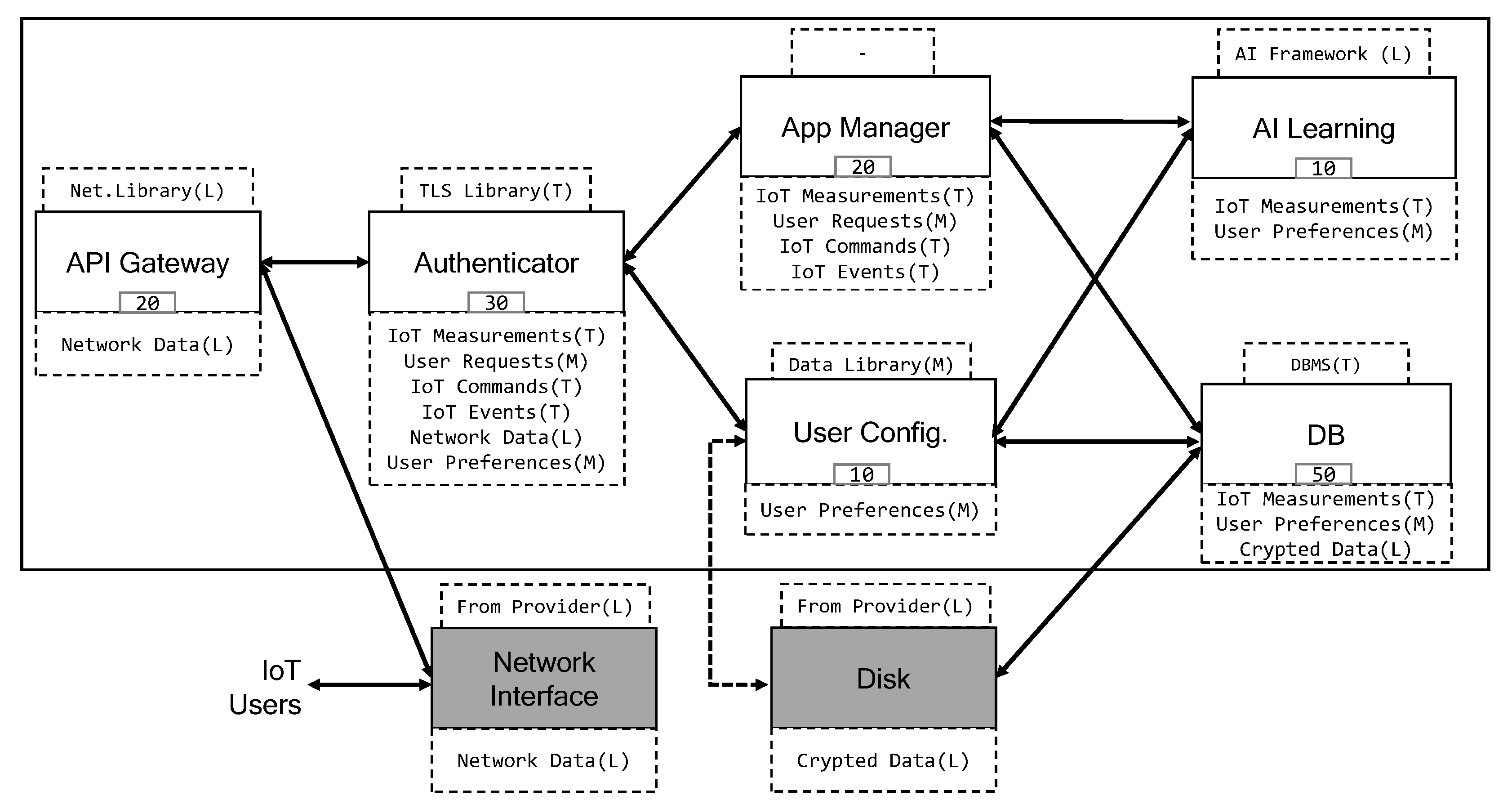
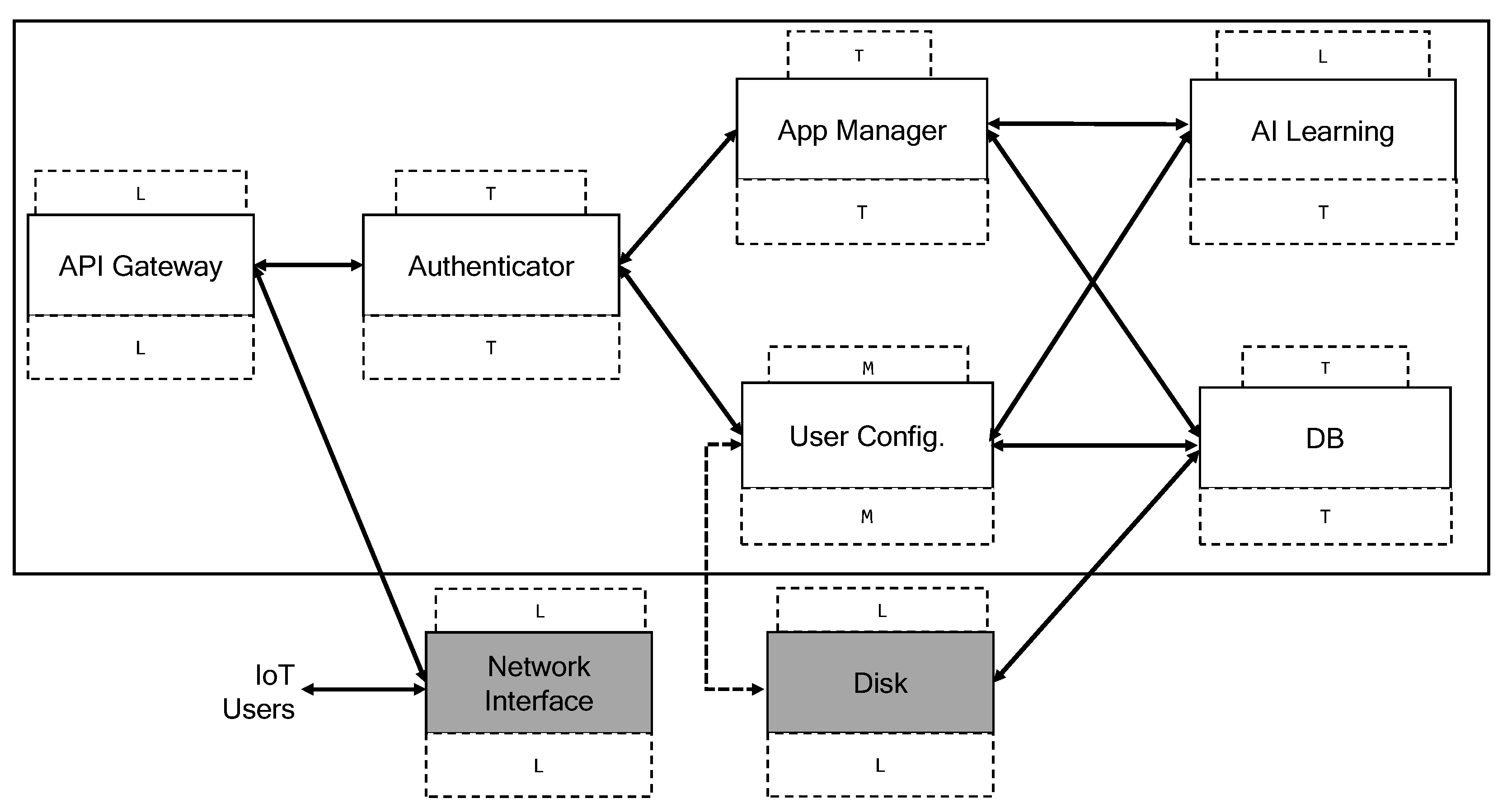
All the experiments were executed sequentially and we collected all the data for this section from the annotated output of ProbSKnife.

The metrics used to evaluate ProbSKnife’s performance and to show the quantitative results about future costs, for each value of K and $DLimit$, are:

• the average execution time to calculate the labelling probabilities, in seconds, calculated over the execution times of the three $DLimit$ values at varying K,
• the execution time to calculate the partitionings and the future costs, in seconds, from the moment to determine the starting partitionings to the end of ProbSKnife execution,
• the future cost, in work hours, given directly by the ProbSKnife output, and
• the probability of having a non-safely partitionable application, also given directly by the ProbSKnife output.

7.1. Experimental Results

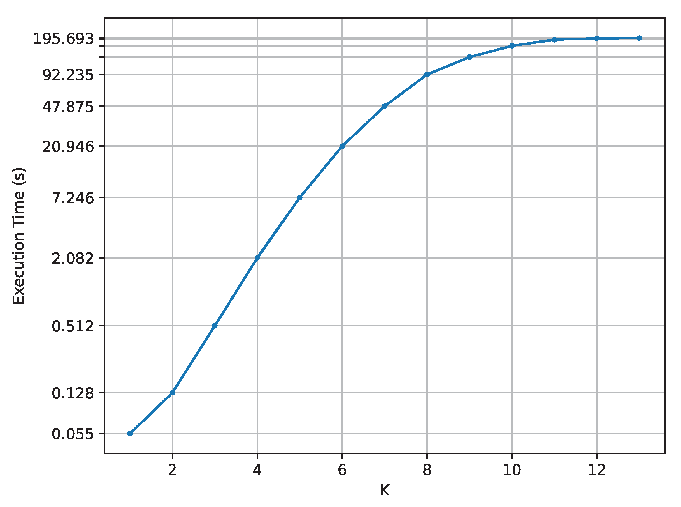
We started by taking the execution time of the probabilistic model creation as K varies. The execution times include the queries to the labellingK predicate and for every labelling, the probability of being in a specific labelling (random variable $Y_i$) and the probability of reaching a labelling from the starting one (random variable $Z_{se}^k$) are computed. Figure 6 shows the average execution time in seconds on a logarithmic scale (y-axis) at varying values of K of each probabilistic model (x-axis).

Increasing K, the execution time grows exponentially, from 55 milliseconds of K equal to 1 to over 3 min of K greater than 11. As aforementioned, for K equal to 11, 12 and 13 the labellings are the same and the difference in execution time is reduced drastically for those values of K.

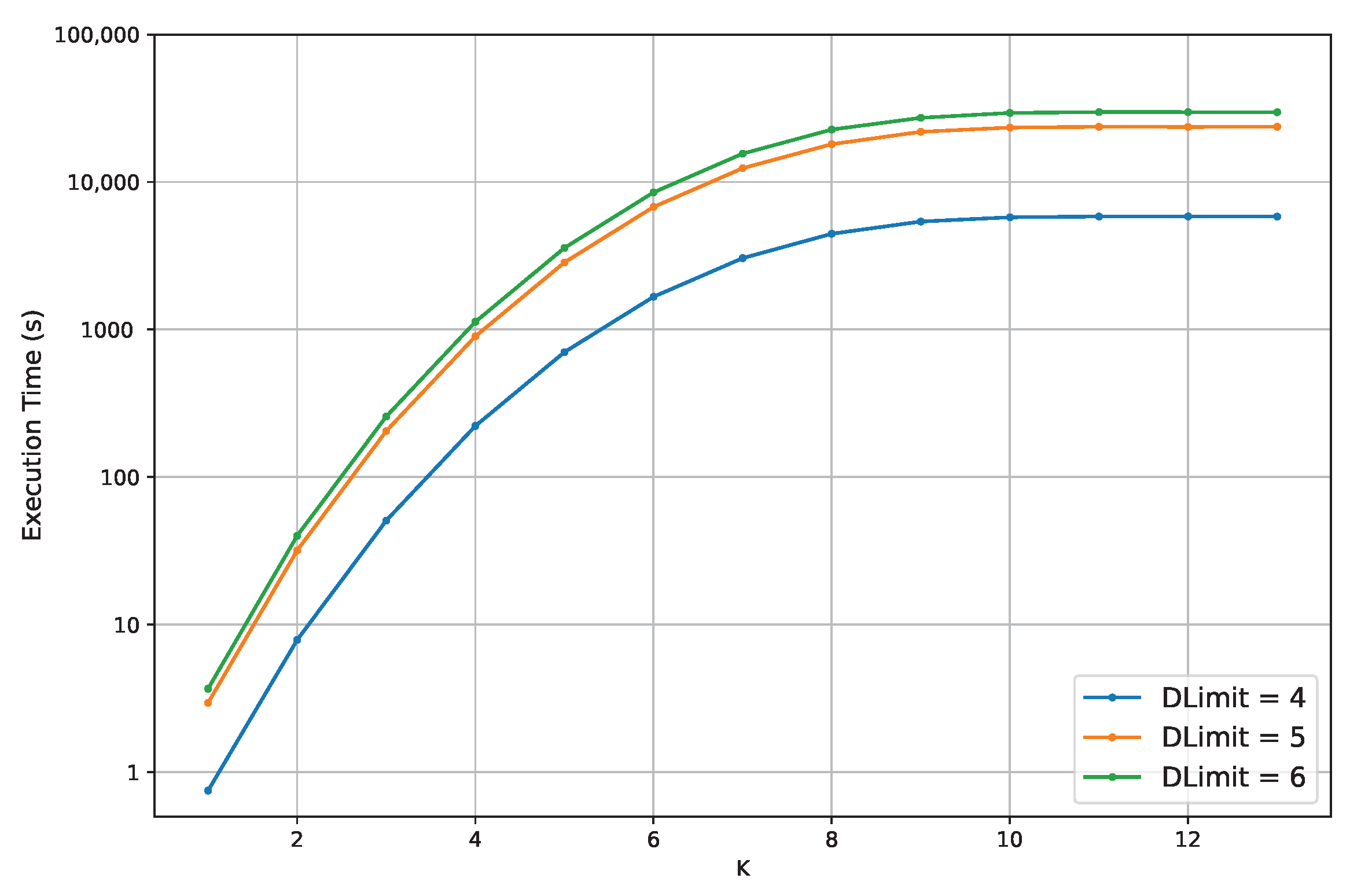
Concerning the total execution time, we collected the data from each experiment and grouped them by $DLimit$. The execution times were obtained by timing the ProbSKnife script after the creation of the probabilistic model. Figure 7 shows the average execution time in seconds on a logarithmic scale (y-axis) at a range of values of K of each probabilistic model (x-axis). The three lines represent the experiments as $DLimit$ varies from four to six. In this plot, the execution time grows exponentially as K varies until K is equal to 11, being on the order of a few seconds for K equal to one and reaching over 8 h (about 28,000 s) for K equal to 13. The three highest values of K have a negligible difference in time, on the order of a few seconds. Concerning the $DLimit$ lines, the execution time for $DLimit$ equal to four is always the lowest, for $DLimit$ equal to five is always the intermediate one and for $DLimit$ equal to six is always the greatest.

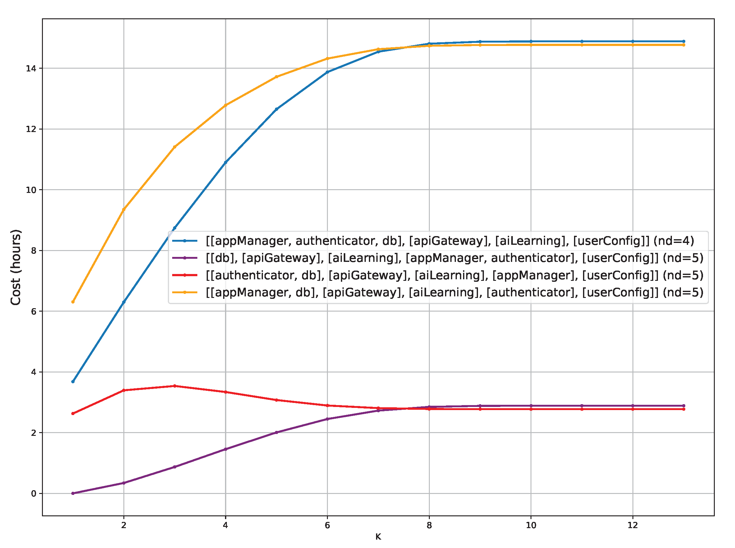
To analyse the partitioning costs we divided the collected data by $DLimit$ to show the future cost as K varies. For each $DLimit$ Figure 8, Figure 9 and Figure 10 show the future cost in work hours (y-axis) at varying values of K of each probabilistic model (x-axis). The number of domains of each partitioning is annotated in the legend as $nd$. In the future cost calculation, the results with K equal to 11, 12 and 13 have the exact same values. As aforementioned, this happens due to the data with a probability of 1 of maintaining the same label. 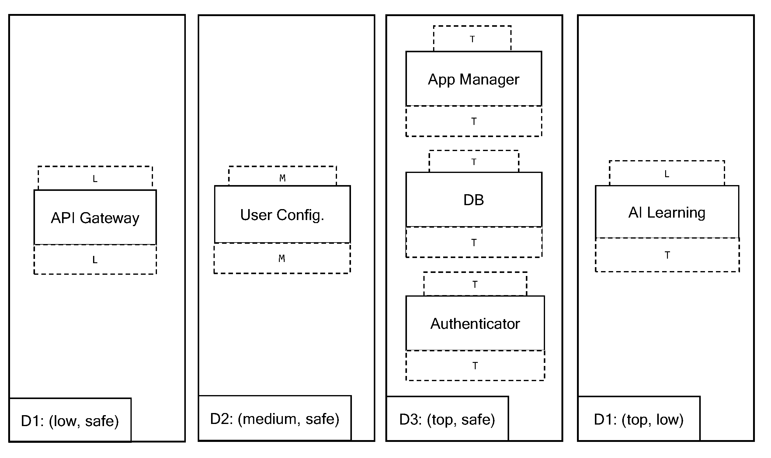We generated three plots with the future cost of a partitioning having the same colour in all the figures; for instance, the minimal partitioning [[appManager,authenticator,db],[apiGateway], [aiLearning],[userConfig]] is always represented with a blue line.

The plot with $DLimit$ equal to four (Figure 8) represents the future cost of only the minimal partitioning. We proved in Section 5 that the solution with the minimum number of domains is unique. The future cost of such a partitioning grows linearly with K, starting from $6.8$ with K equal to one and arriving at a future cost of $16.1$ with K equal to 11, 12 and 13.

The plot with $DLimit$ equal to five (Figure 9) represents the future cost of four different partitionings, the minimal one with four domains and the other with five domains. Two partitionings (the blue and the orange one) have a future cost that grows linearly until K is equal to seven, then it remains stable around 15 h. The blue lines stay under the orange one until that K, and then they switch, with the blue one being the more costly for the highest values of K. The other two partitionings have the same behaviour from K equal to seven onward, but the stabilisation value is around 3 h. With low values of K, the red partitioning starts at $2.6$ h, grows slightly until K is equal to three, reaching a future cost of $3.5$ h, and decreases until K is equal to five, becoming stable at $2.7$ h of future cost. The purple partitioning starts from zero cost, grows slightly until overcoming the red partitioning at K equal to seven and stabilises around a future cost of $2.8$ h. In comparison with the previous plot, the blue partitioning has the same behaviour as before but the values of future cost are always 2 or 3 h less.

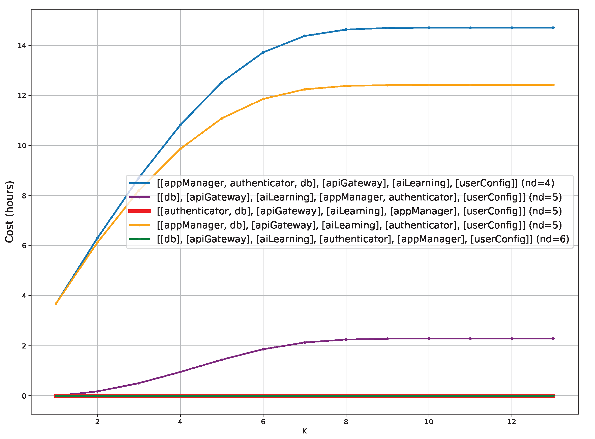
The plot with $DLimit$ equal to six (Figure 10) represents the future cost of five different partitionings, the previous four and the greatest partitioning with all the software components isolated in different domains. To draw this plot the red partitioning has a line slightly bigger than before to avoid hiding the green partitioning because both have a future cost equal to 0 for all the K values. The purple line has the same behaviour as before, but with a future cost value always slightly ($0.2$ to $0.6$ h) less. Differently from before, the orange line is always under the blue line, having the same kind of growth in the cost as K grows but with smaller values, from the minus 1 h with K equal to one until minus 2 with K equal to eight, where it stabilises in both plots.

Finally, we present the results for the probability of having a non-safely partitionable application as K varies. As before, we grouped the data by different $DLimits$. Figure 11 shows the probability of reaching a non-partitionable application (y-axis) at varying values of K of each probabilistic model (x-axis). We drew a line for every value of $DLimit$ with a different size to have a better distinction between the three lines when the probability is similar. Indeed, for $DLimit$ equal to five and six the probability of having a non-safely partitionable application is the same for every K. All three lines start from a probability of $0.175$ with K equal to one and they grow to stabilise with K equal to seven, the blue line at probability $0.535$ and the other two at probability $0.516$. Then, the probability grows with tiny values until K is equal to 11, reaching, respectively, $0.538$ and $0.519$. As before, when K is equal to 11, 12 and 13 all the lines have the same values.

7.2. Discussion of the Results

We discuss now the question

Q1: How much does K impact the creation time of the probabilistic model?

We have to consider that the number of labellings with at most K different labels from the starting labelling grows exponentially as K grows, as discussed in Section 6.1. This behaviour is confirmed by the data shown in Figure 6: the time needed to calculate the probability of each labelling grows exponentially as K grows. With a probabilistic model that is not parameterised with K it could be difficult for ProbSKnife to determine the probabilistic model in a reasonable amount of time. An application with a large number of data types and characteristics has difficulties calculating all the possible labellings, making it hard to calculate the future cost of the initial partitionings. As aforementioned, choosing a low value of K in advance is reasonable given that, in general, the number of labels that change simultaneously is low. We can conclude that having K as a parameter in our methodology can reduce drastically the complexity of the search space for all possible labellings, thus reducing the execution time to create the probabilistic model.

To summarise, the average execution time to create the probabilistic model is exponential with K for the number of labels that can change (11 in our motivating example), with a minimum of $0.055$ seconds with K equal to one and about 195 seconds with K equal to 13.

To answer the question

Q2: How much do K and $DLimit$ impact the execution time of ProbSKnife?

We should add a consideration to the previous one. The maximum number of domains admitted $DLimit$ reduces the number of ways to partition an application and, thus, the number of safe partitionings that satisfy a labelling. Indeed, only one partitioning with $DLimit$ equal to four satisfies the starting labelling (Figure 8). There are four partitionings when $DLimit$ is equal to five (Figure 9) and there are five partitioning when $DLimit$ is equal to six (Figure 10). The number of initial partitionings is the reason behind the difference in the execution times of ProbSKnife, as for different values of $DLimit$ there are different numbers of future costs to calculate. The behaviour of the three lines is the same and they have about the same distance for every point of the plot. This distance is given by the number of partitionings. In particular, the orange line ($DLimit$ equal to five) and the green line ($DLimit$ equal to six) show the time to calculate the future cost of one partitioning, given that they have only one partitioning of difference.

Concerning the behaviour of the execution time, we reach the same conclusion as for the previous question: the value of K increases exponentially the space of possible labellings and ProbSKnife looks for the partitioning with the minimum cost for every labelling, thus increasing the execution time. To summarise, we conclude that increasing K increases the execution time exponentially and increasing $DLimit$ increases the execution time by the number of partitionings that satisfy the starting labelling. This number depends on the application; in the worst-case scenario it is also exponential, as discussed in Section 6.1. Thus, choosing a low value for $DLimit$ exponentially reduces the execution time of ProbSKnife and also decreases the impact on the performance of the separation kernel technology.

To summarise: the average execution time to calculate the initial partitionings and their future costs is exponential with K for the number of labels that can change (11 in our motivating example) and linear with the number of initial partitionings (in the worst case, exponential with $DLimit$). Our results have a minimum of $0.87$ seconds with K and D equal to one and about 28,000 s with K and D at their maximum values, respectively, 13 and six.

From the point of view of execution time, the best choice seems to be the lowest possible values for K and $DLimit$, but we have also to consider their impact on the partitioning costs. In this regard, we now answer the question

Q3: How much do K and $DLimit$ impact the safe partitioning costs?

Having a low value of $DLimit$ reduces the choice for the starting partitioning. Figure 8 shows that having $DLimit$ equal to four has only one partitioning satisfying the starting labelling, the minimal partitioning. Its future cost grows with K because the number of labellings to be satisfied that need a different minimal partitioning grows.

The situation is more interesting with $DLimit$ equal to five, as depicted in Figure 9, where the choice is among four partitionings. The minimal partitioning cost is less than before because when a labelling is not satisfied, the software can also be migrated to partitionings with five domains, with a lower cost than partitioning with four domains. Obviously, the orange partitioning will always be a bad choice, as it is the most costly, with five domains. The choice of the starting partitioning depends on the selected K; the application operator should decide whether to minimise the number of domains—having a higher future cost—or have one more domain with a lower future cost. For example, with K equal to one, the choice is between the purple partitioning (five domains and 0 future cost) and the blue one (four domains and $3.68$ future cost).

The last scenario, with $DLimit$ set to six, is depicted in Figure 10. There is one partitioning more than before, the green one, that is the partitioning where all the software components are isolated in different domains. This partitioning is always safe and always has zero future cost because there is no labelling that forces migration of the software components, but it has the highest number of domains.

For applications with a high number of software components, it is not affordable to isolate all the components and also, in this example, it is not the best choice. The red partitioning has one domain less and the same zero future cost. This happens because changing the partitioning from the red one to the green one has zero cost, so labellings that are not satisfied by the red partitioning are enough to migrate the software to the green one, increasing the number of domains but without paying an additional cost in working on the software communication.

The idea behind the choice of the starting partitioning is the same as before: once K is picked, the application operator should decide how many domains to use at the start, knowing that the migration could require up to six domains to have the minimal cost.

In conclusion, having a low value of K brings lower future costs because the probability of reaching an unsatisfiable labelling is less. Instead, having a low value of $DLimit$ brings higher future costs because there is less choice for the starting partitioning and for the migration.

In summary, fixing $DLimit$ equal to four, the future cost of the minimal partitioning is $6.8$ work hours, the lowest value, when K is equal to one. As K grows over seven the future cost is stabilised at about $16.1$ work hours. Fixing $DLimit$ equal to five, the future cost of the minimal partitioning is $3.7$ work hours, the lowest value, when K is equal to one. As K grows over seven the future cost is stabilised at about $14.8$ work hours. For partitioning with five domains, the behaviour depends on the application architecture and we record as the minimum future cost 0 work hours with K equal to one and $2.7$ with K equal to 13. Finally, fixing $DLimit$ equal to six, the future cost of the minimal partitioning is $3.7$ work hours, the lowest value, when K is equal to one. As K grows over seven the future cost is stabilised at about $14.6$ work hours. For partitioning with five domains, the behaviour depends on the application architecture as before and we record a minimum future cost of 0 work hours for every K. The partitioning with full isolation, having six domains, always has zero future cost.

Finally, we have to answer the question

Q4: How much do K and $DLimit$ impact the probability of not having a safe partitioning?

A labelling does not have a safe partitioning when the application is non-safely partitionable or $DLimit$ is less than the possible configuration of software component labels. We recall that an application is non-safely partitionable when it has untrusted hardware or when there is an untrusted path toward the hardware. When K grows the number of labellings grows exponentially; thus, the probability of having a non-safely partitionable application also grows. This is shown in Figure 11; the three lines grow with K. The growth is bigger at the start, then decreases around K equal to seven. This happens because it is enough to have a few bad labels to have a non-safely partitionable application that can be mitigated with several others. For instance, to make a hardware component untrusted it is enough to have one low characteristic and to make it trusted again all the data need to be low as well.

The lower bound of domains to satisfy all the possible labellings is six. In general, the probability of finding non-satisfiable labellings grows until $DLimit$ reaches the lower bound. For this reason, the figure shows that having the lowest value of $DLimit$ (four) increases the probability of finding non-satisfiable labellings. With $DLimit$ equal to five this does not happen because the labellings that are satisfiable only by six domains make the application non-safely partitionable. Thus, the orange and green lines are overlapping.

To summarise, having a low value of K brings a lower probability of not finding a safe partitioning. When the starting labelling makes the application safely partitionable, having few changes does not increase drastically the probability of making it safely partitionable. Instead, having a low value of $DLimit$ brings a higher probability of not finding a partitioning that satisfies a labelling until the lower bound on the number of domains is reached.

To summarise, the probability of not having an application safely partitionable is the lowest with K equal to one for every $DLimit$, being about $0.175$. With K equal to 13 the probability reaches the maximum of $0.538$ with $DLimit$ equal to four and $0.519$ both with $DLimit$ equal to five and six.

As a final remark, our methodology has the benefit of (i) determining secure deployments of multi-component applications and (ii) proposing different solutions to allow the application operator to choose the trade-off between SK impact and future deployment changes. The main drawback of our methodology resides in the high execution time to handle instances in which applications have several components and a high number of data types and characteristics. To overcome this drawback we give the opportunity to select the K and $DLimit$ parameters to reduce the execution time. According to our experiments:

• Low values of K are suitable to handle problem instances that are likely to incur in a few label changes (e.g., 1–3). In such cases, selecting a low value of K can drastically reduce the execution times, contain future costs and reduce the probability that an application will not be safely partitionable in the future.
• The decision on setting the value of $DLimit$ is less immediate. Low values are suitable to reduce ProbSKnife’s execution time. Instead, high values reduce the future costs and the probability of incurring in a non-safely partitionable application. Assuming that the application deployment is not a latency-sensitive operation, it is advisable to run different instances of ProbSKnife with different $DLimit$ values in order to find the best solution that fits the specific needs of each specific situation.

8. Concluding Remarks and Future Work

This article introduced a declarative methodology to determine safe partitionings of Cloud applications in order to support their secure deployment onto separation kernel technologies, i.e., trusted execution environments.

The methodology is implemented in two Prolog prototypes

• SKnife, which determines the minimal eligible partitioning, the partitioning with the minimum number of domains that satisfies the initial labelling, and
• ProbSKnife, which determines all the eligible partitionings up to a user-defined limit of domains and calculates their future migration cost based on the probability of changing the application labelling.

We introduced the threat model of our considered scenario, which considers unreliable infrastructure providers and external attacks able to compromise the data confidentiality of an arbitrary multi-component application running on Cloud–IoT nodes. Then, we showed how we employ information-flow security to determine eligible partitionings of the application in order to support the deployment onto separation kernel technologies to tackle such threats. We showed how SKnife finds the minimal eligible partitioning and, after introducing our probabilistic cost model, we showed how ProbSKnife determines the eligible partitionings and their future cost parametrised by K—the maximum number of label changes—and DLimit—the maximum number of admitted domains. Finally, we discussed the execution time and the future cost of ProbSKnife varying K and DLimit through experimental assessment.

The results of our experiments show that the execution time of ProbSKnife is exponential in the number of label changes and that bounding K to low values is crucial to have a solution in a reasonable time, reducing it from 8 hours with K = ∞ to milliseconds with K = $1,2$.

Moreover, the results emphasise how it is necessary to have a way to fine-tune the maximum number of admitted DLimits. Too-low values of DLimit reduce the SK impact and the execution time of our prototype. On the other hand, low values of DLimit reduce the number of possible starting deployments and increase the probability of changing the deployment in the future.

To conclude, we highlight three possible directions for future work to enhance our methodology.

Software engineering-based suggestions 

Currently, we deal with non-safely partitionable applications by suggesting relaxed (data or characteristic) labellings. An interesting alternative is to use software engineering techniques to determine modifications of the application architecture in order to avoid data leaks without changing the overall application behaviour. By introducing standard components or architecture patterns, the isolation of untrusted components could be improved and the data could be declassified before sending it to the untrusted components.

Future cost determination 

ProbSKnife computes the exact value of the future cost for all initial safe partitionings. This can be very time-consuming for applications with several components or dealing with a high number of data types and characteristics. An interesting line for future work is to determine an ordering of the partitioning’s future costs, without actually computing their values exactly. We are devising an iterative method that determines boundaries on the probability of migration of partitionings, thus reducing the boundaries at each iterative step in order to contain the execution times.

Mathematical optimisation 

As a last line for future work, we are investigating how to formalise our considered problem as a mixed-integer linear programming problem. This would enable comparing our approach with established optimisation schemes, both from qualitative (viz., application modelling, readability) and quantitative (viz., execution times, solution costs) viewpoints.

References

1. De Donno, M.; Tange, K.; Dragoni, N. Foundations and evolution of modern computing paradigms: Cloud, iot, edge, and fog. IEEE Access 2019, 7, 150936–150948. [Google Scholar] [CrossRef]
2. Kaufman, L.M. Data Security in the World of Cloud Computing. IEEE Secur. Priv. 2009, 7, 61–64. [Google Scholar] [CrossRef]
3. Shaikh, F.B.; Haider, S. Security threats in cloud computing. In Proceedings of the International Conference for Internet Technology and Secured Transactions 2011, Abu Dhabi, United Arab Emirates, 11–14 December 2011; pp. 214–219. [Google Scholar]
4. Mthunzi, S.N.; Benkhelifa, E.; Bosakowski, T.; Guegan, C.G.; Barhamgi, M. Cloud computing security taxonomy: From an atomistic to a holistic view. Future Gener. Comput. Syst. 2020, 107, 620–644. [Google Scholar] [CrossRef]
5. Jangjou, M.; Sohrabi, M.K. A comprehensive survey on security challenges in different network layers in cloud computing. Arch. Comput. Methods Eng. 2022, 29, 3587–3608. [Google Scholar] [CrossRef]
6. Chen, L.; Xian, M.; Liu, J.; Wang, H. Research on virtualization security in cloud computing. In IOP Conference Series: Materials Science and Engineering; IOP Publishing: Bristol, UK, 2020; Volume 806, p. 012027. [Google Scholar]
7. Asvija, B.; Eswari, R.; Bijoy, M. Security in hardware assisted virtualization for cloud computing—State of the art issues and challenges. Comput. Netw. 2019, 151, 68–92. [Google Scholar] [CrossRef]
8. Bennett, K.W.; Robertson, J. Security in the Cloud: Understanding your responsibility. In Cyber Sensing 2019; SPIE: Bellingham, WA, USA, 2019; Volume 11011, p. 1101106. [Google Scholar]
9. Almorsy, M.; Grundy, J.C.; Müller, I. An Analysis of the Cloud Computing Security Problem. arXiv 2016, arXiv:abs/1609.01107. [Google Scholar]
10. Tianfield, H. Security issues in cloud computing. In Proceedings of the 2012 IEEE International Conference on Systems, Man, and Cybernetics (SMC), Seoul, Republic of Korea, 14–17 October 2012; pp. 1082–1089. [Google Scholar]
11. Rushby, J.M. Design and Verification of Secure Systems. In Proceedings of the Eighth Symposium on Operating System Principles SOSP 1981, Pacific Grove, CA, USA, 14–16 December 1981; pp. 12–21. [Google Scholar]
12. Intel Trust Domain Extensions (TDX). Available online: https://www.intel.com/content/www/us/en/developer/articles/technical/intel-trust-domain-extensions.html (accessed on 29 March 2023).
13. AMD Secure Encrypted Virtualization (SEV). Available online: https://developer.amd.com/sev/ (accessed on 29 March 2023).
14. Arm Confidential Compute Architecture (CCA). Available online: https://www.arm.com/why-arm/architecture/security-features/arm-confidential-compute-architecture (accessed on 29 March 2023).
15. Sabt, M.; Achemlal, M.; Bouabdallah, A. Trusted Execution Environment: What It is, and What It is Not. In Proceedings of the 2015 IEEE TrustCom/BigDataSE/ISPA, Helsinki, Finland, 20–22 August 2015; Volume 1, pp. 57–64. [Google Scholar] [CrossRef] [Green Version]
16. Bocci, A.; Guanciale, R.; Forti, S.; Ferrari, G.L.; Brogi, A. Secure Partitioning of Composite Cloud Applications. In Proceedings of the Service-Oriented and Cloud Computing—9th IFIP WG 6.12 European Conference, ESOCC 2022, Wittenberg, Germany, 22–24 March 2022; Lecture Notes in Computer Science; Montesi, F., Papadopoulos, G.A., Zimmermann, W., Eds.; Springer: Berlin/Heidelberg, Germany, 2022; Volume 13226, pp. 47–64. [Google Scholar] [CrossRef]
17. Trach, B.; Oleksenko, O.; Gregor, F.; Bhatotia, P.; Fetzer, C. Clemmys: Towards secure remote execution in FaaS. In Proceedings of the 12th ACM International Conference on Systems and Storage, SYSTOR 2019, Haifa, Israel, 3–5 June 2019; Hershcovitch, M., Goel, A., Morrison, A., Eds.; ACM: New York, NY, USA, 2019; pp. 44–54. [Google Scholar] [CrossRef]
18. Alder, F.; Asokan, N.; Kurnikov, A.; Paverd, A.; Steiner, M. S-FaaS: Trustworthy and Accountable Function-as-a-Service using Intel SGX. In Proceedings of the 2019 ACM SIGSAC Conference on Cloud Computing Security Workshop, CCSW@CCS 2019, London, UK, 11 November 2019; Sion, R., Papamanthou, C., Eds.; ACM: New York, NY, USA, 2019; pp. 185–199. [Google Scholar] [CrossRef] [Green Version]
19. Brenner, S.; Kapitza, R. Trust more, serverless. In Proceedings of the 12th ACM International Conference on Systems and Storage, SYSTOR 2019, Haifa, Israel, 3–5 June 2019; Hershcovitch, M., Goel, A., Morrison, A., Eds.; ACM: New York, NY, USA, 2019; pp. 33–43. [Google Scholar] [CrossRef]
20. Qiang, W.; Dong, Z.; Jin, H. Se-Lambda: Securing Privacy-Sensitive Serverless Applications Using SGX Enclave. In Proceedings of the Security and Privacy in Communication Networks—14th International Conference, SecureComm 2018, Singapore, 8–10 September 2018; Proceedings, Part I, Lecture Notes of the Institute for Computer Sciences, Social Informatics and Telecommunications Engineering; Beyah, R., Chang, B., Li, Y., Zhu, S., Eds.; Springer: Berlin/Heidelberg, Germany, 2018; Volume 254, pp. 451–470. [Google Scholar] [CrossRef]
21. Brenner, S.; Wulf, C.; Goltzsche, D.; Weichbrodt, N.; Lorenz, M.; Fetzer, C.; Pietzuch, P.; Kapitza, R. Securekeeper: Confidential zookeeper using intel sgx. In Proceedings of the 17th International Middleware Conference, Trento, Italy, 12–16 December 2016; pp. 1–13. [Google Scholar]
22. Zheng, W.; Wu, Y.; Wu, X.; Feng, C.; Sui, Y.; Luo, X.; Zhou, Y. A survey of Intel SGX and its applications. Front. Comput. Sci. 2021, 15, 153808. [Google Scholar] [CrossRef]
23. Zhao, C.; Saifuding, D.; Tian, H.; Zhang, Y.; Xing, C. On the Performance of Intel SGX. In Proceedings of the 2016 13th Web Information Systems and Applications Conference (WISA), Wuhan, China, 23–25 September 2016; pp. 184–187. [Google Scholar] [CrossRef]
24. Arfaoui, G.; Gharout, S.; Traoré, J. Trusted Execution Environments: A Look under the Hood. In Proceedings of the 2014 2nd IEEE International Conference on Mobile Cloud Computing, Services, and Engineering, Oxford, UK, 8–11 August 2014; pp. 259–266. [Google Scholar] [CrossRef]
25. Lind, J.; Priebe, C.; Muthukumaran, D.; O’Keeffe, D.; Aublin, P.; Kelbert, F.; Reiher, T.; Goltzsche, D.; Eyers, D.; Kapitza, R.; et al. Glamdring: Automatic Application Partitioning for Intel SGX; USENIX: Berkeley, CA, USA, 2017. [Google Scholar]
26. Brumley, D.; Song, D. Privtrans: Automatically partitioning programs for privilege separation. In Proceedings of the USENIX Security Symposium, San Diego, CA, USA, 9–13 August 2004; Volume 57. [Google Scholar]
27. Gudka, K.; Watson, R.N.; Anderson, J.; Chisnall, D.; Davis, B.; Laurie, B.; Marinos, I.; Neumann, P.G.; Richardson, A. Clean application compartmentalization with SOAAP. In Proceedings of the 22nd ACM SIGSAC Conference on Computer and Communications Security, Denver, CO, USA, 12–16 October 2015; pp. 1016–1031. [Google Scholar]
28. Wu, Y.; Sun, J.; Liu, Y.; Dong, J.S. Automatically partition software into least privilege components using dynamic data dependency analysis. In Proceedings of the 2013 28th IEEE/ACM International Conference on Automated Software Engineering (ASE), Silicon Valley, CA, USA, 11–15 November 2013; pp. 323–333. [Google Scholar] [CrossRef]
29. Bittau, A.; Marchenko, P.; Handley, M.; Karp, B. Wedge: Splitting Applications into Reduced-Privilege Compartments; USENIX Association: Berkeley, CA, USA, 2008. [Google Scholar]
30. Liu, Y.; Zhou, T.; Chen, K.; Chen, H.; Xia, Y. Thwarting memory disclosure with efficient hypervisor-enforced intra-domain isolation. In Proceedings of the 22nd ACM SIGSAC Conference on Computer and Communications Security, Denver, CO, USA, 12–16 October 2015; pp. 1607–1619. [Google Scholar]
31. Watson, P. A Multi-Level Security Model for PartitioningWorkflows over Federated Clouds. In Proceedings of the 2011 IEEE Third International Conference on Cloud Computing Technology and Science, Athens, Greece, 29 November–1 December 2011; pp. 180–188. [Google Scholar] [CrossRef]
32. Sewell, T.; Winwood, S.; Gammie, P.; Murray, T.C.; Andronick, J.; Klein, G. seL4 Enforces Integrity. In Proceedings of the Interactive Theorem Proving: Second International Conference, ITP 2011, Berg en Dal, The Netherlands, 22–25 August 2011; Springer: Berlin/Heidelberg, Germany, 2011; Volume 6898, pp. 325–340. [Google Scholar]
33. Andronick, J. From a Proven Correct Microkernel to Trustworthy Large Systems. In Proceedings of the FoVeOOS, Paris, France, 28–30 June 2010; Springer: Berlin/Heidelberg, Germany, 2010; Volume 6528, pp. 1–9. [Google Scholar]
34. Dam, M.; Guanciale, R.; Khakpour, N.; Nemati, H.; Schwarz, O. Formal verification of information flow security for a simple arm-based separation kernel. In Proceedings of the 2013 ACM SIGSAC Conference on Computer & Communications Security 2013, Berlin, Germany, 4–8 November 2013; pp. 223–234. [Google Scholar]
35. Heitmeyer, C.L.; Archer, M.; Leonard, E.I.; McLean, J.D. Formal specification and verification of data separation in a separation kernel for an embedded system. In Proceedings of the 13th ACM Conference on Computer and Communications Security 2006, Alexandria, VA, USA, 30 October–3 November 2006; pp. 346–355. [Google Scholar]
36. Rubinov, K.; Rosculete, L.; Mitra, T.; Roychoudhury, A. Automated partitioning of android applications for trusted execution environments. In Proceedings of the 38th International Conference on Software Engineering, Austin, TX, USA, 14–22 May 2016; pp. 923–934. [Google Scholar]
37. Sabelfeld, A.; Sands, D. A Per Model of Secure Information Flow in Sequential Programs. High. Order Symb. Comput. 2001, 14, 59–91. [Google Scholar] [CrossRef]
38. Elsayed, M.; Zulkernine, M. IFCaaS: Information Flow Control as a Service for Cloud Security. In Proceedings of the 2016 11th International Conference on Availability, Reliability and Security (ARES), Salzburg, Austria, 31 August–2 September 2016; pp. 211–216. [Google Scholar]
39. Alpernas, K.; Flanagan, C.; Fouladi, S.; Ryzhyk, L.; Sagiv, M.; Schmitz, T.; Winstein, K. Secure serverless computing using dynamic information flow control. Proc. ACM Program. Lang. 2018, 2, 118:1–118:26. [Google Scholar] [CrossRef] [Green Version]
40. Datta, P.; Kumar, P.; Morris, T.; Grace, M.; Rahmati, A.; Bates, A. Valve: Securing Function Workflows on Serverless Computing Platforms. In Proceedings of the WWW, Taipei, Taiwan, 20–22 April 2020; pp. 939–950. [Google Scholar]
41. Bocci, A.; Forti, S.; Ferrari, G.L.; Brogi, A. Declarative Secure Placement of FaaS Orchestrations in the Cloud-Edge Continuum. Electronics 2023, 12, 1332. [Google Scholar] [CrossRef]
42. Oak, A.; Ahmadian, A.M.; Balliu, M.; Salvaneschi, G. Language Support for Secure Software Development with Enclaves. In Proceedings of the IEEE Computer Security Foundations Symposium (CSF 2021), Dubrovnik, Croatia, 21–25 June 2021. [Google Scholar]
43. Kadioglu, S.; Colena, M.; Sebbah, S. Heterogeneous resource allocation in Cloud Management. In Proceedings of the NCA 2016, Boston, MA, USA, 31 October–2 November 2016; pp. 35–38. [Google Scholar]
44. Hinrichs, T.L.; Gude, N.S.; Casado, M.; Mitchell, J.C.; Shenker, S. Practical declarative network management. In Proceedings of the WREN, Barcelona, Spain, 21 August 2009; pp. 1–10. [Google Scholar]
45. Forti, S.; Ferrari, G.L.; Brogi, A. Secure Cloud-Edge Deployments, with Trust. Future Gener. Comput. Syst. 2020, 102, 775–788. [Google Scholar] [CrossRef]
46. Forti, S.; Paganelli, F.; Brogi, A. Probabilistic QoS-aware Placement of VNF chains at the Edge. Theory Pract. Log. Program. 2022, 22, 1–36. [Google Scholar]
47. Sahita, R.; Caspi, D.; Huntley, B.; Scarlata, V.; Chaikin, B.; Chhabra, S.; Aharon, A.; Ouziel, I. Security analysis of confidential-compute instruction set architecture for virtualized workloads. In Proceedings of the 2021 International Symposium on Secure and Private Execution Environment Design (SEED), Washington, DC, USA, 20–21 September 2021; pp. 121–131. [Google Scholar]
48. Sabelfeld, A.; Myers, A.C. Language-based information-flow security. IEEE J. Sel. Areas Commun. 2003, 21, 5–19. [Google Scholar] [CrossRef] [Green Version]
49. Home Assistant. Available online: https://www.home-assistant.io/ (accessed on 29 March 2023).
50. IFTTT. Available online: https://ifttt.com/ (accessed on 29 March 2023).
51. AWS IoT Greengrass. Available online: https://aws.amazon.com/it/greengrass/ (accessed on 29 March 2023).
52. Azure IoT Edge. Available online: https://azure.microsoft.com/en-us/services/iot-edge/ (accessed on 29 March 2023).
53. Dey, T.; Ma, Y.; Mockus, A. Patterns of Effort Contribution and Demand and User Classification Based on Participation Patterns in NPM Ecosystem. In Proceedings of the Fifteenth International Conference on Predictive Models and Data Analytics in Software Engineering. Association for Computing Machinery PROMISE’19, Athens, Greece, 19–20 August 2019; pp. 36–45. [Google Scholar] [CrossRef] [Green Version]
Figure 1. Application architecture (labels: T = top, M = medium, L = low).
Futureinternet 15 00224 g001
Figure 2. Overview of SKnife methodology.
Futureinternet 15 00224 g002
Figure 3. Labelling of application components.
Futureinternet 15 00224 g003
Figure 4. Minimal safe partitioning.
Futureinternet 15 00224 g004
Figure 5. Partitioning change due to Authenticator labelling change.
Futureinternet 15 00224 g005
Figure 6. Execution times for computing labelling probabilities at varying K.
Futureinternet 15 00224 g006
Figure 7. Execution times for computing expected costs at varying K and DLimit.
Futureinternet 15 00224 g007
Figure 8. Future costs at varying K for 4 domains.
Futureinternet 15 00224 g008
Figure 9. Future costs at varying K for at most 5 domains.
Futureinternet 15 00224 g009
Figure 10. Future costs at varying K for at most 6 domains.
Futureinternet 15 00224 g010
Figure 11. Probability of non-safely partitionable application with varying K and number of domains.
Futureinternet 15 00224 g011