Latency-Aware Semi-Synchronous Client Selection and Model Aggregation for Wireless Federated Learning

Abstract

Federated learning (FL) is a collaborative machine-learning (ML) framework particularly suited for ML models requiring numerous training samples, such as Convolutional Neural Networks (CNNs), Recurrent Neural Networks (RNNs), and Random Forest, in the context of various applications, e.g., next-word prediction and eHealth. FL involves various clients participating in the training process by uploading their local models to an FL server in each global iteration. The server aggregates these models to update a global model. The traditional FL process may encounter bottlenecks, known as the straggler problem, where slower clients delay the overall training time. This paper introduces the Latency-awarE Semi-synchronous client Selection and mOdel aggregation for federated learNing (LESSON) method. LESSON allows clients to participate at different frequencies: faster clients contribute more frequently, therefore mitigating the straggler problem and expediting convergence. Moreover, LESSON provides a tunable trade-off between model accuracy and convergence rate by setting varying deadlines. Simulation results show that LESSON outperforms two baseline methods, namely FedAvg and FedCS, in terms of convergence speed and maintains higher model accuracy compared to FedCS.

1. Introduction

With the development of the Internet of Things (IoT), numerous smart devices, such as smartphones, smartwatches, and virtual-reality headsets, are widely used to digitize people’s daily lives. Traditionally, a huge volume of data generated by these IoT devices is uploaded to and analyzed by a centralized data center that generates high-level knowledge and provides corresponding services to users, thus facilitating their lives [1]. A typical example is smart homes, where various IoT devices, such as smart meters, thermostats, motion detectors, and humidity sensors, are deployed to monitor the status of the smart homes. The data generated by the IoT devices would be uploaded to a centralized data center, which applies a deep reinforcement learning model to intelligently and autonomously control, for example, the smart bulbs and air conditioners in smart homes, to improve the quality of experience and reduce the energy usage of smart homes [2].

On the other hand, sharing data with third-party data centers may raise privacy concerns as data generated by IoT devices may contain personal information, such as users’ locations and personal preferences [3]. As a result, various policies have been made, such as General Data Protection Regulation (GDPR) made by the European Union [4], to regulate and hinder data sharing. To fully utilize these personal data while preserving privacy (i.e., without sharing the data), federated learning (FL) is proposed to distributively train machine-learning models by enabling different IoT devices to analyze their data locally without uploading them to a central facility [5]. A typical example of using FL is to train a next-word prediction model, which is used to predict what word comes next based on the existing text information [6]. Basically, as shown in Figure 1, an FL server would first initialize the parameters of the global model and then broadcast the global model to all the clients via wireless networks. Each client would train the received global model based on its local data sets (i.e., their text messages) and upload the updated model to the FL server via wireless networks. The FL server then aggregates the received models from the clients to generate a new global model and then starts a new iteration by broadcasting the new global model to the clients. The iteration continues until the model is converged.

The traditional FL method can resolve the privacy issue to allow the clients to train the model locally, and it applies the synchronous strategy, where the FL server must wait until it receives the models from all the clients in each global iteration. This may lead to the straggler problem when the configurations of clients are heterogeneous, meaning that they have different computing and communications capabilities. Hence, some stragglers take much longer time to train and upload their models in a global iteration because of their lower computing and communications capabilities, and thus significantly prolong the model training process. To resolve the straggler problem, many client selection methods have been proposed [7,8,9,10,11,12], which would select the qualified clients that can finish their model training and uploading before a predefined deadline. Normally, client selection and resource allocation are jointly optimized to maximize the number of selected qualified clients. Selecting qualified clients can resolve the straggler problem but may raise other issues. First, the proposed client selection may significantly reduce the number of participating clients, which may slow down the convergence speed [13], thus leading to longer training latency (which equals the sum of the latency for all the global iterations). Second, the proposed client selection may result in the model overfitting issue caused by the reduction of data diversity, i.e., if the FL server only selects the qualified clients to participate in the model training, then the generated model can only fit the data samples in these qualified clients, but not the non-qualified clients. The model overfitting issue would be compounded if the data samples of the qualified clients are not sufficient [14]. The other solution to solve the straggler problem is to apply asynchronous FL, where the FL server does not need to wait until the deadline expires for each global iteration but would update the global model once it receives a local model from a client [15]. However, the asynchronous FL may suffer from (1) the high communications cost since both the FL server and clients will more frequently exchange their models and (2) the stale issue, where some slow clients are training based on an outdated global model, which may lead to slow convergence rate or even global model divergence [16,17].

To solve the slow convergence and model overfitting issues in the synchronous FL while avoiding model divergence in the asynchronous FL, we propose a semi-synchronous FL method, i.e., Latency awarE Semi-synchronous client Selection and mOdel aggregation for federated learNing (LESSON). The basic idea of LESSON is to allow all the clients to participate in the whole learning process with different frequencies. Specifically, the clients are clustered into different tiers based on their model training and uploading latency. The clients in a lower tier (i.e., lower model training and uploading latency) would participate in the learning process more frequently than those in a higher tier (with higher model training and uploading latency). As a result, the straggler problem can be resolved (since the FL server does not need to wait for stragglers in each global iteration), and the model overfitting problem can be fixed (since all the clients join the learning process to provide high data diversity). The main contributions of the paper are summarized as follows.

• A new semi-synchronous FL algorithm, i.e., LESSON, is introduced. LESSON introduces a latency-aware client clustering technique that groups clients into different tiers based on their computing and uploading latency. LESSON allows all the clients in the system to participate in the training process but at different frequencies, depending on the clients’ associated tiers. LESSON is expected to mitigate the straggler problem in synchronous FL and model overfitting in asynchronous FL, thus expediting model convergence.
• LESSON also features a specialized model aggregation method tailored to client clustering. This method sets the weight and timing for local model aggregation for each client tier.
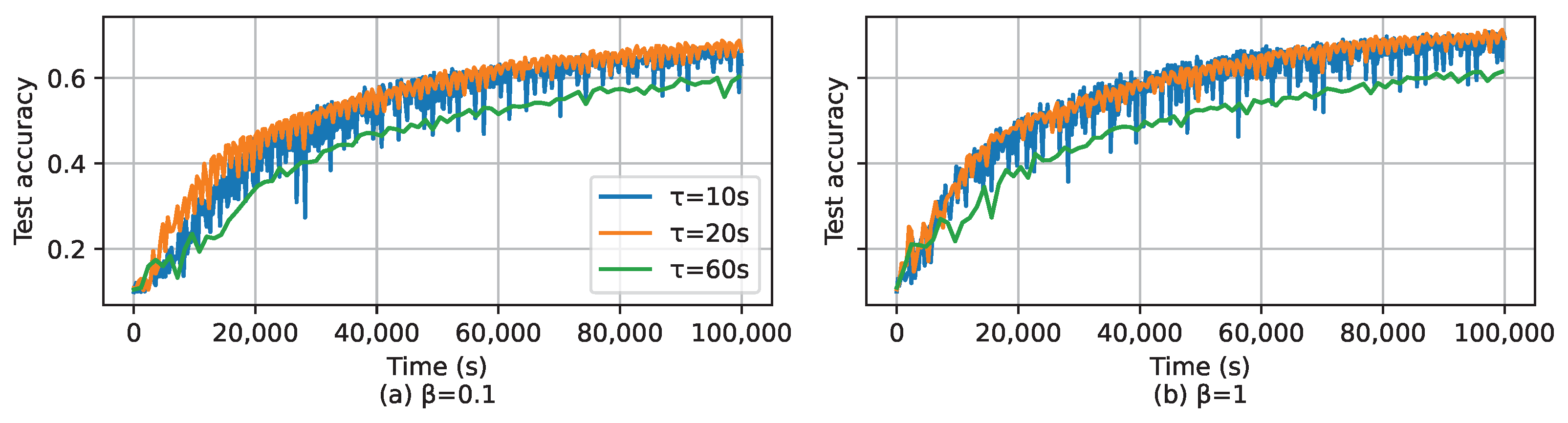
• The proposed LESSON algorithm also integrates the dynamic model aggregation and step size adjustment according to client clustering and offers flexibility in balancing model accuracy and convergence speed by adjusting the deadline $\tau$.
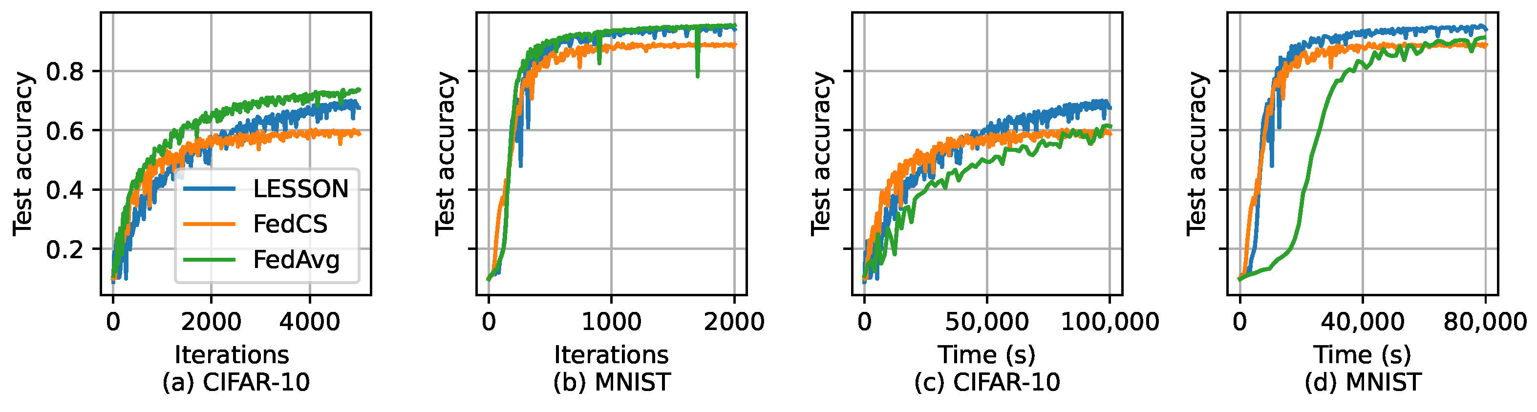
• Extensive experimental evaluations show that LESSON outperforms FedAvg and FedCS in terms of faster convergence and higher model accuracy.

The rest of this paper is organized as follows. The related work is summarized in Section 2. System models are described in Section 3. Section 4 elaborates on the proposed LESSON algorithm, which comprises client clustering and model aggregation. In Section 5, the performance of LESSON is compared with the other two baseline algorithms via extensive simulations, and simulation results are analyzed. Finally, Section 6 concludes this paper.

2. Related Work

Solving the straggler issue is one of the main challenges in synchronous FL. The existing solutions mainly focus on jointly optimizing client selection and resource allocation. Nishio and Yonetani [18] aimed to maximize the number of selected clients that can finish their model training and uploading before a predefined deadline in each global iteration. By assuming that the selected clients must iteratively upload their models to the FL server, they designed FedCS that jointly optimizes the uploading schedule and client selection to achieve the objective. Abdulrahman and Tout [19] designed a similar client selection method FedMCCS. The goal of FedMCCS is to maximize the number of selected clients who can not only finish the model training and uploading before a predefined deadline but also guarantee the resource utilization is less than the threshold to avoid device dropout. Albelaihi et al. [11] proposed a client selection method that tries to achieve the same objective as FedCS, but they argued that the latency of a client in waiting for the wireless channel to be available for model uploading should be considered; otherwise, the selected clients may not upload their local models before the deadline. Yu et al. [20] proposed to dynamically adjust and optimize the trade-off between maximizing the number of selected clients and minimizing the total energy consumption of the selected clients by picking suitable clients and allocating appropriate resources (in terms of CPU frequency and transmission power) in each global iteration. Shi et al. [21] also jointly optimized the client selection and resource allocation for FL. However, the objective is to minimize the overall learning latency (which equals the product of the average latency of one global iteration and the number of global iterations) while achieving a certain model accuracy. They formulated a system model to estimate the number of global iterations given the global model accuracy requirement. All the mentioned client selection methods for synchronous FL can alleviate the straggler problem but may lead to a slow convergence rate and model overfitting issues, as we illustrated previously.

Instead of selecting qualified clients to avoid stragglers, Li et al. [22] proposed to let fast clients train their local models by running more gradient descent iterations in each global iteration. In this way, the fast and slow clients could upload their models at a similar time, but the fast clients may provide better models to fit their local data samples, thus potentially speeding up the model convergence. This method, however, may lead to local model overfitting issues when some fast clients run too many gradient descent iterations over the limited data samples. The overfitted local models would significantly slow down the global model convergence. Wu et al. [23] proposed to perform spilt learning, where a global neural network is divided into two parts. The parameters in the former and latter layers are trained in the clients and the FL server, respectively. As a result, the computational complexity of the clients is reduced, thus potentially reducing the training time and energy consumption of the clients.

Other works aim to design asynchronous FL, where the FL server does not need to wait for the selected clients to upload their local models; instead, once the FL server receives a local model from a client, it would aggregate the received local model to update the global model, and then send the updated global model to the client [24,25,26,27]. However, as mentioned before, the fast clients and the FL server must exchange their models more frequently, thus leading to higher communications costs for both the fast clients and FL server [28,29]. Meanwhile, in asynchronous FL, the slower clients may train their local models based on an outdated global model, which results in slow convergence or even leads to model divergence [30,31].

To overcome the drawbacks in synchronous and asynchronous FL, we propose the semi-synchronous FL to allow all the clients to participate in the whole learning process with different frequencies. Although the term “semi-synchronous FL” has been used by the existing works, the definitions are different from what we defined in this paper. For example, Stripelis and Ambite [32] defined semi-synchronous FL as the clients train their local models over different sizes of local data sets, depending on their computing capabilities. The semi-synchronous FL proposed in [33] periodically re-selects a number of clients and follows the same method as asynchronous FL to aggregate and update the global model.

3. System Models

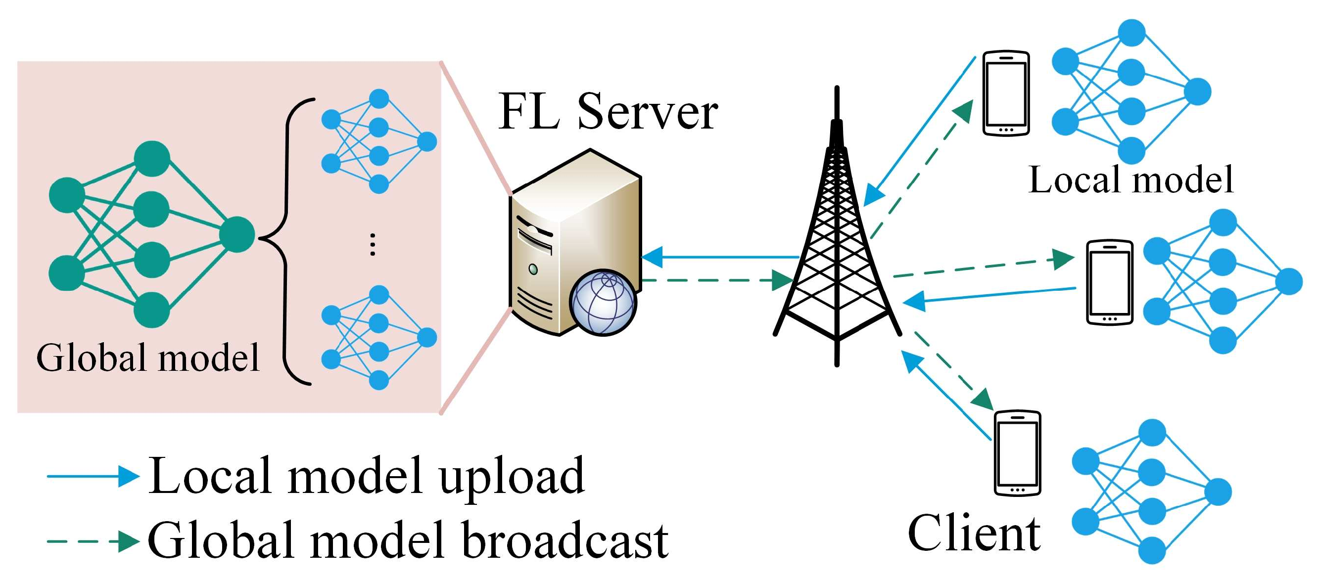
3.1. Federated Learning Preliminary

The idea of FL is to enable distributed clients to cooperatively train a global model such that the global loss function, denoted as $\mathcal{F}\left(\mathbf{\omega }\right)$, can be minimized. That is,

$${\displaystyle \underset{\mathbf{\omega }}{argmin}}\mathcal{F}\left(\mathbf{\omega }\right)={\displaystyle \underset{\mathbf{\omega }}{argmin}}{\displaystyle \sum _{i\in \mathcal{I}}}\frac{\left|{\mathcal{D}}_i\right|}{\left|\mathcal{D}\right|}{f}_i\left(\mathbf{\omega }\right),$$

(1)

where $\mathbf{\omega }$ is the set of the parameters for the global model, $\mathcal{I}$ is the set of the selected clients, $\left|\mathcal{D}\right|$ is the number of the training data samples of all the clients, $\left|{\mathcal{D}}_i\right|$ is the number of the training data samples at client i (where $\mathcal{D}={\displaystyle \bigcup _{i\in \mathcal{I}}}{\mathcal{D}}_i$), and $f_i\left(\mathbf{\omega }\right)$ is the local loss function of client i, i.e.,

$$f_i\left(\mathbf{\omega }\right)=\frac{1}{\left|{\mathcal{D}}_i\right|}{\displaystyle \sum _{n\in {\mathcal{D}}_i}}f\left(\mathbf{\omega },{\mathbf{a}}_{i,n},b_{i,n}\right).$$

(2)

Here, $\left({\mathbf{a}}_{i,n},b_{i,n}\right)$ is the input-output pair for the $nth$ data sample in user i’s data set, and $f\left(\mathbf{\omega },{\mathbf{a}}_{i,n},b_{i,n}\right)$ captures the error of the local model (with parameter $\mathbf{\omega }$) over $\left({\mathbf{a}}_{i,n},b_{i,n}\right)$.

In each global iteration, FL comprises four steps.

• Server broadcast: In the k-th global iteration, the FL server broadcasts the global model generated in the previous global iteration, denoted as ${\mathbf{\omega }}^{\left(k-1\right)}$, to all the selected clients.
• Client local training: Each client i trains its local model over its local data set ${\mathcal{D}}_i$, i.e., ${\mathbf{\omega }}_i^{\left(k\right)}={\mathbf{\omega }}_i^{\left(k-1\right)}-\delta \nabla f_i\left({\mathbf{\omega }}_i^{\left(k-1\right)}\right)$, where $\delta$ is the learning rate.
• Client model uploading: After deriving the local model ${\mathbf{\omega }}_i^{\left(k\right)}$, client i uploads its local model to the FL server.
• Server model aggregation: The FL server aggregates the local models from the clients and updates the global model based on, for example, FedAvg [5], i.e., ${\mathbf{\omega }}^{\left(k\right)}={\displaystyle \sum _{i\in \mathcal{I}}}\frac{\left|{\mathcal{D}}_i\right|}{\left|\mathcal{D}\right|}{\mathbf{\omega }}_i^{\left(k\right)}$.

The global iteration keeps executed to update the global model ${\mathbf{\omega }}^{\left(k\right)}$ until the global model converges.

3.2. Latency Models of a Client

There are four steps in each global iteration for FL, and so the latency of a global iteration equals the sum of the latency among these four steps. The local model training latency in Step (2) and local model uploading latency in Step (3) are different among the clients, depending on their computing and communications capacities. In addition, the global model broadcast latency in Step (1) and model aggression latency in Step (4) are the same for all the clients and are normally negligible as compared to local model training and uploading latency. Thus, we define the latency of client i in a global iteration as follows.

$$t_i=t_i^{comp}+t_i^{upload},$$

(3)

where $t_i^{comp}$ is the computing latency of client i in training its local model over its local data samples in Step (2), and $t_i^{upload}$ is the uploading latency of client i in uploading its local model to the FL server in Step (3).

3.2.1. Computing Latency

The computing latency of client i in a global iteration can be estimated by [34]

$$t_i^{comp}=\theta {log}_2\left(\frac{1}{ϵ}\right)\frac{C_i\left|{\mathcal{D}}_i\right|}{f_i},$$

(4)

where $\theta$ is a constant determined by the structure of the desired model; $\theta {log}_2\left(\frac{1}{ϵ}\right)$ indicates the estimated number of local iterations to achieve the required training accuracy $ϵ$; $C_i$ in cycles/sample is the number of CPU cycles required for training one data sample of the local model; $\left|{\mathcal{D}}_i\right|$ is the number of training samples used by client i; $f_i$ in cycles/second is CPU frequency of client i, which is determined by the device hardware.

3.2.2. Uploading Latency

The achievable data rate of client i can be estimated by

$$r_i=b{log}_2\left(1+\frac{p{g}_i}{N_0}\right),$$

(5)

where b is the amount of bandwidth allocated to each participating client, p is the transmission power of the client, $g_i$ is the channel gain from client i to the BS calculated, and $N_0$ is the average background noise and inter-cell interference power density. We assume that the size of the local model is s, and so the latency of client i in uploading its local model to the BS is

$$t_i^{upload}=\frac{s}{r_i}=\frac{s}{b{log}_2\left(1+\frac{p{g}_i}{N_0}\right)}.$$

(6)

4. Latency-awarE Semi-Synchronous Client Selection and mOdel Aggregation for Federated learNing (LESSON)

In contrast to synchronous FL, the proposed LESSON method aims to allow all the clients to participate in the whole learning process while avoiding the straggler problem. The basic idea of LESSON is to cluster the clients into different tiers based on their latency and the deadline. The clients in different tiers would train and upload their local models at different frequencies.

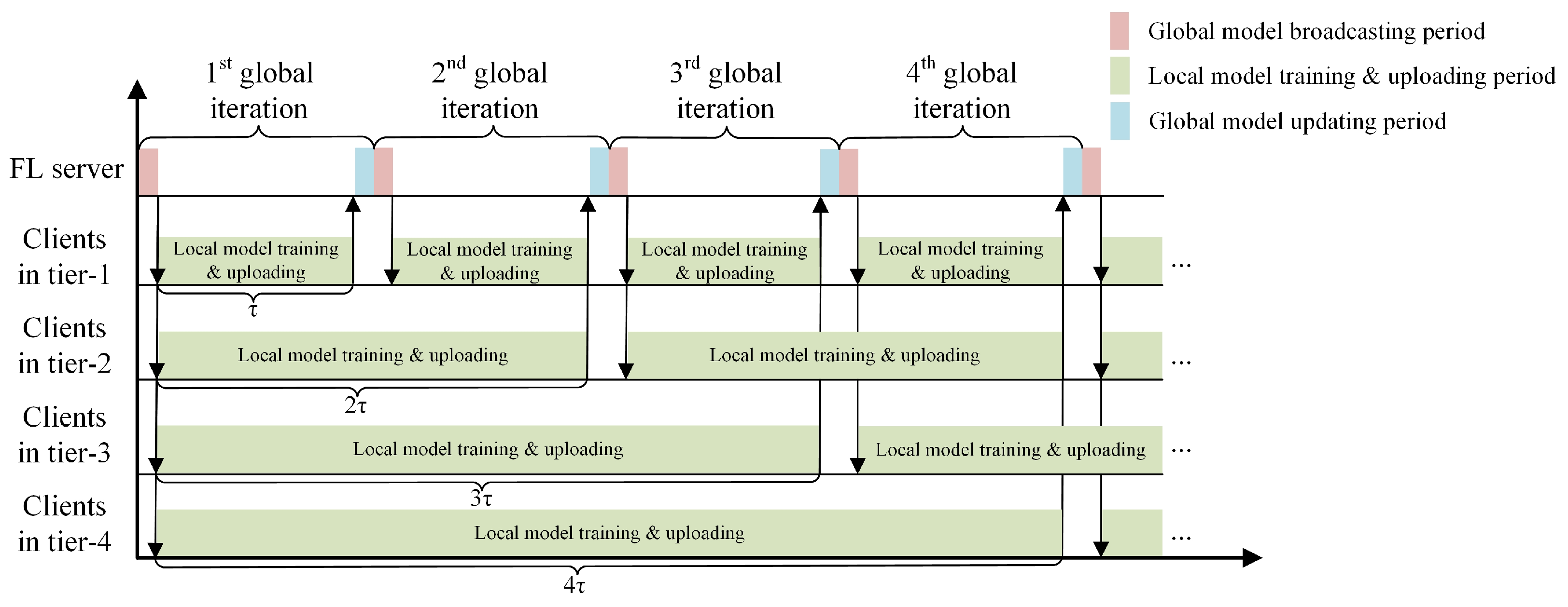
4.1. Latency-Aware Client Clustering

We denote $\tau$ as the deadline of a global iteration. The FL server would accept all the models uploaded from the clients before the deadline $\tau$ and reject the rest in each global iteration. Hence, we cluster the clients into several tiers, and $x_{ij}$ is used to indicate whether client i is in Tier j (i.e., $x_{ij}=1$) or not (i.e., $x_{ij}=0$). Basically, if client i can finish its local model training and uploading before deadline $\tau$, i.e., $t_i\le \tau$, then client i is in Tier 1, i.e., $x_{i1}=1$. Similarly, if client i can finish its local model training and uploading between $\tau$ and $2\times \tau$, i.e., $\tau <t_i\le 2\times \tau$, then client i is in Tier 2, i.e., $x_{i2}=1$. The following equation provides a general mathematical expression to cluster client i into a specific tier.

$$\begin{array}{c}\hfill x_{ij}=\left\{\begin{array}{cc}1,\hfill & \mathrm{if}\tau \times (j-1)<t_i\le \tau \times j,\hfill \\ 0,\hfill & \mathrm{otherwise},\hfill \end{array}\right.\end{array}$$

(7)

where j is the index of tiers.

4.2. Semi-Synchronized Model Aggregation

In each global iteration, clients from different tiers upload their local models, and the FL server can estimate when a client may upload its local model according to its associated tier. Figure 2 provides one example to illustrate the scheduling of the clients from four tiers in LESSON. For example, the clients in Tier 1 are expected to upload their local models in each global iteration, and the clients in Tier 2 are expected to upload their local models in every two global iterations. Denote k as the index of the global iterations, and let $y_{jk}$ be the binary variable to indicate whether the clients in Tier j are expected to upload their local models by the end of $k^{th}$ global iteration, where

$$\begin{array}{c}\hfill y_{jk}=\left\{\begin{array}{cc}1,\hfill & \mathrm{if}k\%j=0,\hfill \\ 0,\hfill & \mathrm{otherwise},\hfill \end{array}\right.\end{array}$$

(8)

where % is the modulo operation, and so $k\%j=0$ indicates k is divisible by j. Meanwhile, let $z_{ik}$ be the binary variable to indicate whether client i is expected to upload its local model by the end of $kth$ global iteration ($z_{ik}=1$) or not ($z_{ik}=0$), where

$$z_{ik}=x_{ij}{y}_{jk}.$$

(9)

Based on the value of $z_{ik}$, the FL server would expect which clients will upload their local models in global iteration k, and then aggregate all the received local models based on

$${\mathbf{\omega }}^{\left(k\right)}={\displaystyle \sum _{i\in \mathcal{I}}}\frac{\left|{\mathcal{D}}_i\right|}{{\displaystyle \sum _{i\in \mathcal{I}}}\left|{\mathcal{D}}_i\right|z_{ik}}{\mathbf{\omega }}_i^{\left(k\right)}{z}_{ik},$$

(10)

where ${\displaystyle \sum _{i\in \mathcal{I}}}\left|{\mathcal{D}}_i\right|z_{ik}$ indicates the total number of the data samples among all the clients, who would upload their local models in global iteration k.

Please note that, in synchronous FL (e.g., FedAvg), each selected client would update its local model ${\mathbf{\omega }}_i^{\left(k\right)}$ based on Equation (11) in each global iteration.

$${\mathbf{\omega }}_i^{\left(k\right)}={\mathbf{\omega }}_i^{\left(k-1\right)}-\delta \nabla f_i\left({\mathbf{\omega }}_i^{\left(k-1\right)}\right),$$

(11)

where $\delta$ is the step size, which is the same for all the selected clients. In LESSON, different clients update their local models in different frequencies, depending on their associated tiers, so it is reasonable to adopt different step sizes for the clients in different tiers [24]. Here, we adjust the step size of a client proportional to its tier (i.e., $\delta \times j$). Thus, when $k\%j=0$, client i in Tier j would update its local model based on

$${\mathbf{\omega }}_i^{\left(k\right)}={\mathbf{\omega }}_i^{\left(k-j\right)}-j\delta \nabla f_i\left({\mathbf{\omega }}_i^{\left(k-j\right)}\right)$$

(12)

4.3. Summary of LESSON

Algorithm 1 provides an overview of the LESSON algorithm. Initially, the FL server estimates the latency of all the clients and clusters the clients into different tiers based on Equation (7), i.e., Steps 1–2 in Algorithm 1. Then, the FL server broadcasts the initial global model ${\mathbf{\omega }}^{\left(0\right)}$ to start the collaborative model training process, which unfolds over numerous global iterations.

Within each global iteration k, each client trains and updates its local model ${\mathbf{\omega }}_i^{\left(k\right)}$ based on Equation (12). If $z_{ik}=1$, client i should upload its local model to the FL server by the end of global iteration k. Then, client i would wait until it receives the updated global model ${\mathbf{\omega }}^{\left(k\right)}$ from the FL server to start the next round of local model training.

Concurrently, the FL server keeps receiving the local models from the clients in global iteration k. Once the deadline expires, the FL server updates the global model ${\mathbf{\omega }}^{\left(k\right)}$ based on Equation (10), and then broadcasts the new global model ${\mathbf{\omega }}^{\left(k\right)}$ to the clients, who just uploaded their local models in global iteration k.

Please note that the deadline of a global iteration, i.e., $\tau$, is a very crucial parameter to adjust the performance of LESSON. Specifically, if $\tau \to +\infty$, a single tier is employed, housing all clients. This setup operates akin to the FedAvg. Here, the FL server must patiently await the arrival of local models from all clients during each global iteration.

Conversely, if $\tau \to 0$, LESSON acts as asynchronous FL, where clients with varying latency (i.e., $t_i$) are distributed across distinct tiers. The FL server will promptly aggregate the local models from the clients with low latency, subsequently updating and broadcasting the global model. This adaptability in $\tau$ constitutes one of LESSON’s strengths, and we will delve into how different values of $\tau$ impact LESSON’s performance in Section 5.

Algorithm 1: LESSON algorithm

5. Simulation

In this section, we conduct extensive simulations to evaluate the performance of LESSON.

5.1. Simulation Setup

5.1.1. Configuration of Clients

We assume that there are 50 clients that are uniformly distributed in a 2 km × 2 km area, which is covered by a BS located at the center of the area. All the clients upload their local models to the FL server via the BS. The pathloss between the BS and client i is calculated based on $128.1+37.6\times d_i$, where $d_i$ is the distance in kilometer between the BS and client i. Then, the channel gain is calculated based on $g_i={10}^{-(128.1+37.6\times d_i)/10}$ [35]. Meanwhile, the transmission power $p_i$ is set to be 1 Watt for all the clients, and the amount of available bandwidth for each client in uploading its local model is 30 kHz. In addition, each client has around $\left|{\mathcal{D}}_i\right|=1000$ data samples (i.e., 50,000 combined for all clients) to train its local model. The number of CPU cycles required for training one data sample (i.e., $C_i$) among clients is randomly selected from a uniform distribution, i.e., $C_i\sim \mathcal{U}\left(3,5\right)\times {10}^5$ CPU cycles/sample. The CPU frequency of a client $f_i$ is also randomly selected from a uniform distribution, i.e., $f_i\sim \mathcal{U}\left(0.8,3\right)$ GHz. Other simulation parameters are listed in

Table 1. Simulation parameters.

Parameter	Value
Noise and inter-cell interference ($N_0$)	$-94$ dBm
Bandwidth B	30 kHz
Transmission power	0.1 watt
Size of the local model (s)	100 kbit
Number of local iterations $\left(\theta {log}_2\left(\frac{1}{ϵ}\right)\right)$	$1\times {log}_2\left(\frac{1}{0.05}\right)$
Number of local samples $\left|{\mathcal{D}}_i\right|$	1000
CPU cycles required for training one data sample $C_i$	$\mathcal{U}\left(3,5\right)\times {10}^8$
CPU frequency $f_i$	$\mathcal{U}\left(0.8,3\right)$ GHz
Number of local epochs	1
Number of local batch size	20
Non-IID Dirichlet distribution parameter $\beta$	$[0.1,1,10]$
Client Learning Rate $\delta ,$	$0.02$

.

Figure 3 shows the probability density function of the latency (i.e., $t_i$) among all the clients in a specific time instance. The median value in the clients’ latency is around 10 s, so we initially set up the deadline $\tau$ of a global iteration to be 10 s, and we will change the value of $\tau$, later, to see how it affects the performance of LESSON.

5.1.2. Machine-Learning Model and Training Datasets

We will use two benchmark datasets to train the corresponding machine-learning model.

• CIFAR-10 [36] is an image classification dataset containing 10 labels/classes of images, each of which has 6000 images. Among the 60,000 images, 50,000 are used for model training and 10,000 for model testing.
• MNIST [37] is a handwritten digit dataset that includes many $28\times 28$ pixel grayscale images of handwritten single digits between 0 and 9. The whole dataset has a training set of 60,000 examples and a test set of 10,000 examples.

We apply the convolutional neural network (CNN) to classify the CIFAR-10 images. The CNN model has four 3 × 3 convolution layers (where the first layer has 32 channels, and each of the following three layers has 64 channels. Also, only the first two layers are followed with $2\times 2$ max pooling), followed by a dropout layer with rate of 75%, a fully connected 256 units ReLU layer, and a 10-unit SoftMax output layer. There are a total of 1,144,650 parameters in this CNN model.

With respect to MNIST, which is a much simpler image dataset than CIFAR-10, a smaller CNN model has been used. Specifically, the CNN model has two 5 × 5 convolution layers (where the two layers have 6 and 16 channels, respectively, each of which is followed with a $2\times 2$ max pooling), followed with two fully connected ReLU layers with 120 and 84 units, respectively, and a 10-unit SoftMax output layer. There are a total of 61,706 parameters in this CNN model.

In addition, we partition the MNIST/CIFAR-10 dataset among the 50 clients based on the non-independent and identical distribution (Non-IID), and the probability of having ${\eta }_m$ images in label class m at client i is assumed to follow a Dirichlet distribution [38], i.e.,

$$f({\eta }_1,{\eta }_2,\cdots ,{\eta }_M;\beta )=\frac{\mathsf{\Gamma }\left(\beta M\right)}{\mathsf{\Gamma }{\left(\beta \right)}^M}\prod _{m=1}^M{\eta }_m^{\beta -1},$$

(13)

where M is the total number of label classes (i.e., $M=10$ for both CIFAR-10 and MNIST), $\mathsf{\Gamma }\left(\right)$ is the gamma function ($\mathsf{\Gamma }\left(z\right)={\int }_0^{\infty }{x}^{z-1}{e}^{-x}dx$), and $\beta$ is the concentration parameter that determines the level of label imbalance. A larger $\beta$ results in a more balanced data partition among different labels within a client (i.e., much closer to IID) and vice versa. Figure 4 shows how different labels of images are distributed by varying $\beta$. In addition, we assume each client would train its CNN model over $\left|{\mathcal{D}}_i\right|=20$ data samples locally based on stochastic gradient descent (SGD) with base learning rate $\delta =0.1$ [39] and epoch equal to 1.

5.1.3. Baseline Comparison Methods

The performance of LESSON will be compared with the other two baseline client selection algorithms, i.e., FedCS [18] and FedAvg [13]. FedCS only selects the clients that can finish their model uploading before the deadline $\tau$ in each global iteration, i.e., only the clients in Tier 1 will be selected to participate in the training process. In FedAvg, all the clients in the network will be selected to participate in the training process for each global iteration, i.e., the FL server will wait until it receives the local models from all the clients and then update the global model for the next global iteration. In addition, the source code of LESSON can be found in https://github.com/fzvincent/FL_AoR/tree/master (accessed on 29 September 2023).

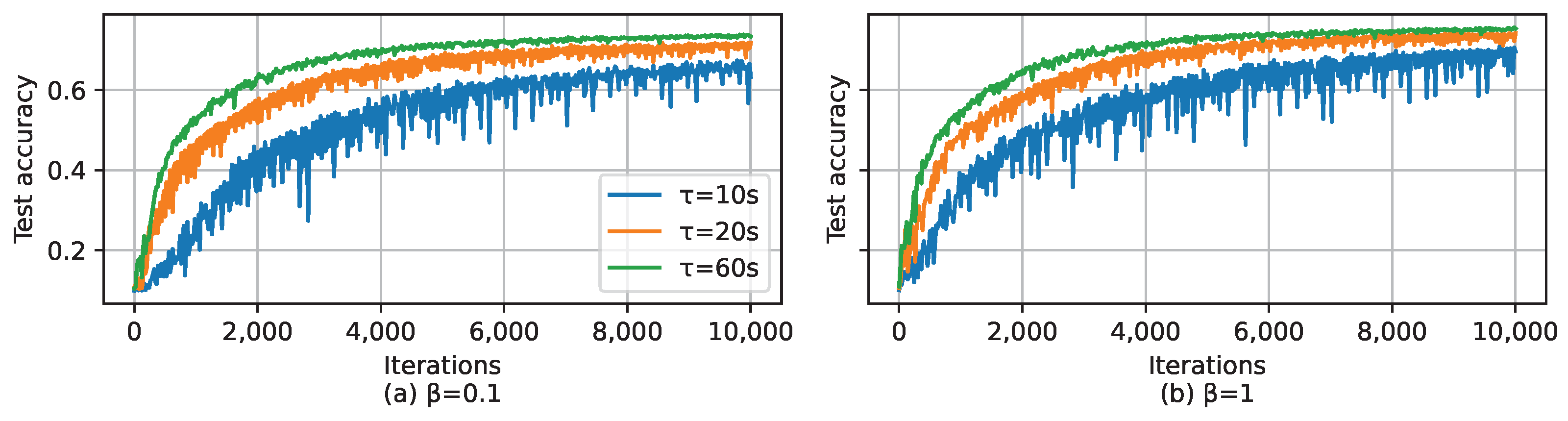
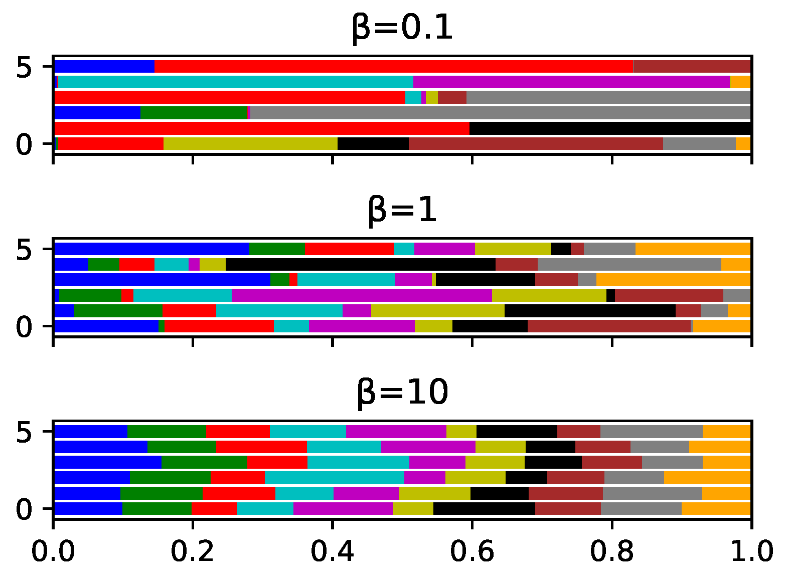
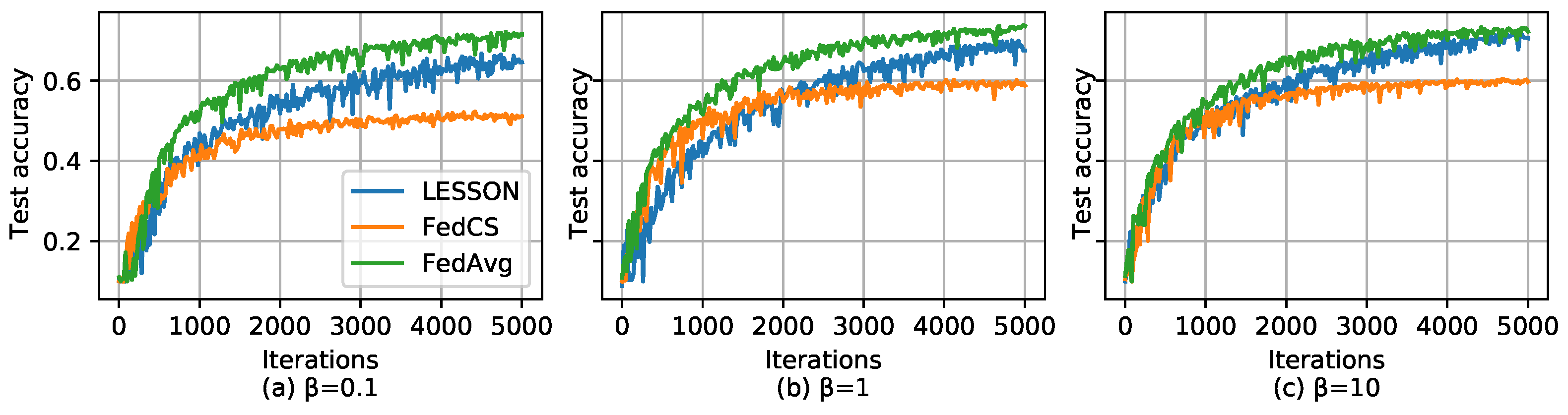
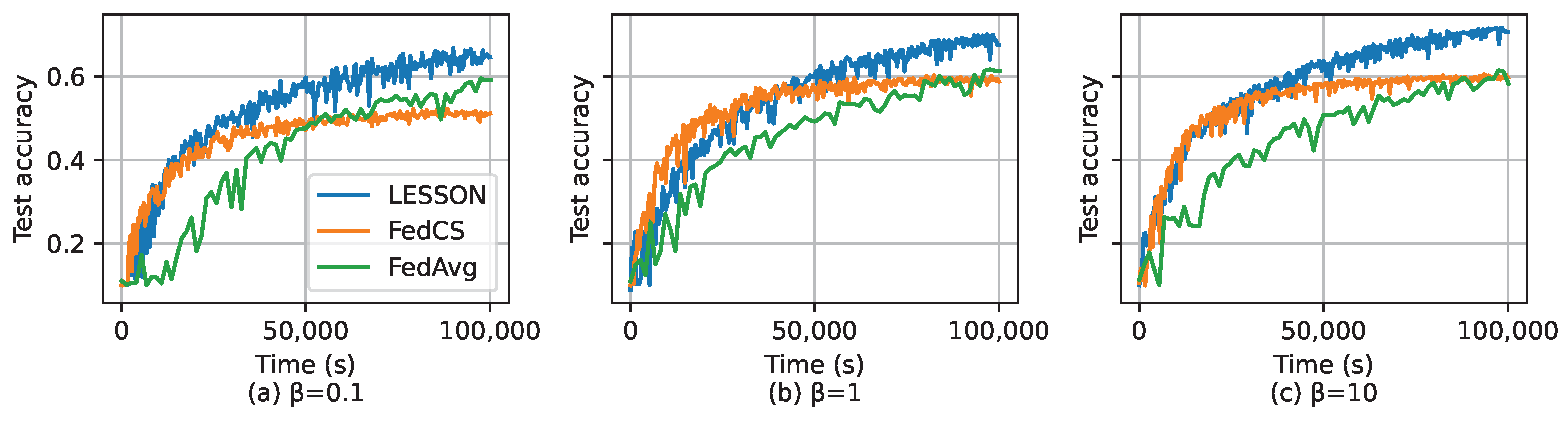
5.2. Simulation Results

Assume that $\beta =1$ and $\tau =20$ s. Figure 5 shows the test accuracy of the three algorithms over the global iterations and simulation time for CIFAR-10 and MNIST. From Figure 5a,b, we can find that LESSON and FedAvg have similar test accuracy, i.e., ∼70% for CIFAR-10 and ∼95% for MNIST. However, the test accuracy achieved by FedCS is lower than LESSON and FedAvg, i.e., ∼60% for CIFAR-10 and ∼90% for MNIST. This is because FedCS only selects fast clients to participate in the training process, and so the derived global model can only fit the data samples for fast clients, not slow clients, thus reducing the model accuracy. Meanwhile, the convergence rate with respect to the number of global iterations for LESSON and FedAvg is also very similar, which is slightly faster than FedCS. However, by evaluating the convergence rate with respect to the time, as shown in Figure 5c,d, we find out that LESSON is faster than FedAvg. For example, the global model in LESSON has already converged at 20,000 s for MNIST, but the global model in FedAvg is still under-trained. This is because the FL server in FedAvg must wait until the local models from all the clients have been received in each global iteration, and thus, the latency of a global iteration incurred by FedAvg is much higher than that incurred by LESSON.

Table 2. Average latency per global iteration for different algorithms.

Algorithms	Average Latency of a Global Iteration
FedAvg	68 s
FedCS	20 s
LESSON	20 s

shows the average delay of a global iteration incurred by different algorithms, where the average latency of a global iteration incurred by LESSON is 48 s faster than FedAvg. As a result, FedAvg only runs around 588 global iterations at 20,000 s in Figure 5d, respectively, but LESSON runs 2000 global iterations.

We further investigate how the data sample distribution affects the performance of the algorithms based on CIFAR-10. As mentioned before, $\beta$ is used to change the data sample distribution, i.e., a larger $\beta$ implies a more balanced data partition among the labels in a client or data sample distribution much closer to IID, and vice versa. Assume $\tau =20$ seconds, and Figure 6 shows the test accuracy of different algorithms over the number of global iterations by selecting different values of $\beta$. From the figures, we can see that if the data sample distribution exhibits non-IID, i.e., $\beta =0.1$, FedAvg has higher test accuracy than LESSON and FedCS. As $\beta$ increases, i.e., the data sample distribution is growing closer to IID, the test accuracy gap between FedAvg and LESSON is growing smaller, while the test accuracy of FedCS remains unchanged. On the other hand, Figure 7 shows the test accuracy of different algorithms over time by selecting different values of $\beta$. From the figure, we can see that LESSON achieves $2\times$ faster convergence rate than FedAvg under different values of $\beta$. Therefore, we conclude that LESSON achieves a faster convergence rate at the cost of slightly reducing the model accuracy, especially when the data distribution exhibits non-IID.

As mentioned in Section 4.3, the deadline of a global iteration, i.e., $\tau$, is a very important parameter to adjust the performance of LESSON. Basically, if $\tau \to +\infty$, LESSON acts as FedAvg, and if $\tau \to 0$, LESSON acts as asynchronous FL. Figure 8 shows the test accuracy of LESSON by having different values of $\tau$ and $\beta$ for CIFAR-10 over global iterations, where we can find that $\tau =60$ seconds incurs the highest test accuracy for both $\beta =0.1$ and $\beta =1$. This is because a larger $\tau$ (1) reduces the number of tiers in the system, thus alleviating the performance degradation caused by stale issues, and (2) increases the average number of clients in uploading their local models in a global iteration, which can mitigate the impact caused by non-IID. Also, we can see that the blue curve, i.e., $\tau =10$ s, is more sensitive to the change in $\beta$ than the other two curves. This is because as $\tau$ reduces, LESSON acts more like asynchronous FL, which has the convergence issue under non-IID. Figure 9 shows the test accuracy of LESSON by having different values of $\tau$ and $\beta$ for CIFAR-10 over time. From Figure 9a, we can find that $\tau =60$ exhibits the slowest convergence rate with respect to the time because a larger $\tau$ implies a longer latency of a global latency, i.e., $\tau =60$ runs the fewest global iterations than $\tau =10$ and $\tau =20$ within a time period. Therefore, we conclude that changing $\tau$ can adjust the trade-off between the model accuracy and model convergence rate with respect to time. A large $\tau$ can increase the model accuracy but reduce the model convergence rate, and vice versa. Meanwhile, as the data distribution is closer to IID (i.e., as $\beta$ increases), the difference in the convergence rate among the three algorithms increases, as shown in Figure 9b.

The two foundational approaches select clients based on their availability. FedAvg emphasizes the importance of client presence but suffers from delays caused by slow participants, known as stragglers. On the other hand, FedCS prioritizes models that have been recently updated. LESSON integrates the strengths of both approaches: it places stragglers in higher tiers to minimize system disruption and effectively incorporates less up-to-date models to enhance the global model’s generalization capability. When dealing with clients who drop out intermittently, FedAvg can experience significant delays, and FedCS does not account for the contributions of clients with unstable connections in the first place. Although LESSON cannot offer guarantees, it provides an opportunity for such disconnected clients to make a partial contribution to the global model.

6. Conclusions

To address challenges related to data diversity and stragglers in synchronous Federated Learning (FL) while also minimizing the risk of model divergence found in asynchronous FL, we introduce LESSON. This novel approach blends semi-synchronous client selection with model aggregation, ensuring the participation of all clients in the FL process, albeit at differing frequencies.

The simulation results show that LESSON and FedAvg have comparable model test accuracy, both of which outperform FedCS at least $10\%$ under different non-IID scenarios. In addition, LESSON reduces the test accuracy by around 5% but accelerates convergence rate at least $2\times$ faster as compared to FedAvg. The adaptability of LESSON is further highlighted through its deadline parameter $\tau$, which allows for adjusting the trade-off between model accuracy and convergence rate, that higher $\tau$ can improve model accuracy. Due to the high convergence rate, LESSON can be applied to applications that require quickly deriving a reasonable model adaptive to dynamic environments, such as autonomous drone swarm control [40,41], where actor-critic networks that can be adaptive to be the current wind perturbation should be quickly trained and derived to, for example, avoid collisions.

Future work is poised to delve into the adaptive modification of the $\tau$ parameter to augment LESSON’s performance. This paper has demonstrated that a lower $\tau$ accelerates the model convergence rate, whereas a higher $\tau$ achieves a better model accuracy, especially in non-IID data scenarios. As such, dynamically calibrating $\tau$ to achieve a resilient and practical FL algorithm is critical but unexplored. In addition, the computing and uploading latency of a client may change over time. If a client moves towards the edge of a base station’s coverage area, the uploading latency of this client will be significantly increased. As a result, this client will finally be clustered into a higher tier to train and upload its local model at a lower pace but with a higher learning rate. Yet, how LESSON dynamically adjusts the client clustering based on the updated computing and uploading latency and how the client clustering adjustment affects the performance of LESSON is still unveiled and will be part of our future work.

References

1. Sun, X.; Ansari, N. EdgeIoT: Mobile Edge Computing for the Internet of Things. IEEE Commun. Mag. 2016, 54, 22–29. [Google Scholar] [CrossRef]
2. Liu, Y.; Yang, C.; Jiang, L.; Xie, S.; Zhang, Y. Intelligent Edge Computing for IoT-Based Energy Management in Smart Cities. IEEE Netw. 2019, 33, 111–117. [Google Scholar] [CrossRef]
3. Dhanvijay, M.M.; Patil, S.C. Internet of Things: A survey of enabling technologies in healthcare and its applications. Comput. Netw. 2019, 153, 113–131. [Google Scholar] [CrossRef]
4. Goddard, M. The EU General Data Protection Regulation (GDPR): European regulation that has a global impact. Int. J. Mark. Res. 2017, 59, 703–705. [Google Scholar] [CrossRef]
5. McMahan, B.; Moore, E.; Ramage, D.; Hampson, S.; y Arcas, B.A. Communication-Efficient Learning of Deep Networks from Decentralized Data. In Proceedings of the 20th International Conference on Artificial Intelligence and Statistics, Lauderdale, FL, USA, 20–22 April 2017; PMLR: Cambridge, MA, USA, 2017; pp. 1273–1282. [Google Scholar]
6. Hard, A.; Rao, K.; Mathews, R.; Ramaswamy, S.; Beaufays, F.; Augenstein, S.; Eichner, H.; Kiddon, C.; Ramage, D. Federated learning for mobile keyboard prediction. arXiv 2018, arXiv:1811.03604. [Google Scholar]
7. Imteaj, A.; Amini, M.H. Fedar: Activity and resource-aware federated learning model for distributed mobile robots. In Proceedings of the 2020 19th IEEE International Conference on Machine Learning and Applications (ICMLA), Miami, FL, USA, 14–17 December 2020; pp. 1153–1160. [Google Scholar]
8. Wu, W.; He, L.; Lin, W.; Mao, R.; Maple, C.; Jarvis, S. SAFA: A semi-asynchronous protocol for fast federated learning with low overhead. IEEE Trans. Comput. 2020, 70, 655–668. [Google Scholar] [CrossRef]
9. Reisizadeh, A.; Tziotis, I.; Hassani, H.; Mokhtari, A.; Pedarsani, R. Straggler-resilient federated learning: Leveraging the interplay between statistical accuracy and system heterogeneity. arXiv 2020, arXiv:2012.14453. [Google Scholar] [CrossRef]
10. Xu, Z.; Yang, Z.; Xiong, J.; Yang, J.; Chen, X. Elfish: Resource-aware federated learning on heterogeneous edge devices. Ratio 2019, 2, r2. [Google Scholar]
11. Albelaihi, R.; Sun, X.; Craft, W.D.; Yu, L.; Wang, C. Adaptive Participant Selection in Heterogeneous Federated Learning. In Proceedings of the 2021 IEEE Global Communications Conference (GLOBECOM), Madrid, Spain, 7–11 December 2021; pp. 1–6. [Google Scholar] [CrossRef]
12. Tang, T.; Ali, R.E.; Hashemi, H.; Gangwani, T.; Avestimehr, S.; Annavaram, M. Adaptive Verifiable Coded Computing: Towards Fast, Secure and Private Distributed Machine Learning. In Proceedings of the 2022 IEEE International Parallel and Distributed Processing Symposium (IPDPS), Lyon, France, 30 May–3 June 2022; pp. 628–638. [Google Scholar] [CrossRef]
13. Wang, J.; Joshi, G. Cooperative SGD: A unified framework for the design and analysis of communication-efficient SGD algorithms. arXiv 2018, arXiv:1808.07576. [Google Scholar]
14. Shorten, C.; Khoshgoftaar, T.M. A survey on image data augmentation for deep learning. J. Big Data 2019, 6, 1–48. [Google Scholar] [CrossRef]
15. Li, L.; Fan, Y.; Lin, K.Y. A survey on federated learning. In Proceedings of the 2020 IEEE 16th International Conference on Control & Automation (ICCA), Singapore, 9–11 October 2020; pp. 791–796. [Google Scholar]
16. Xu, C.; Qu, Y.; Xiang, Y.; Gao, L. Asynchronous federated learning on heterogeneous devices: A survey. arXiv 2021, arXiv:2109.04269. [Google Scholar] [CrossRef]
17. Damaskinos, G.; Guerraoui, R.; Kermarrec, A.M.; Nitu, V.; Patra, R.; Taiani, F. FLeet: Online Federated Learning via Staleness Awareness and Performance Prediction. In Proceedings of the 21st International Middleware Conference, Delft, The Netherlands, 7–11 December 2020; Association for Computing Machinery: New York, NY, USA, 2020. Middleware ’20. pp. 163–177. [Google Scholar] [CrossRef]
18. Nishio, T.; Yonetani, R. Client Selection for Federated Learning with Heterogeneous Resources in Mobile Edge. In Proceedings of the 2019 IEEE International Conference on Communications (ICC), Shanghai, China, 20–24 May 2019; pp. 1–7. [Google Scholar] [CrossRef]
19. Abdulrahman, S.; Tout, H.; Mourad, A.; Talhi, C. FedMCCS: Multicriteria Client Selection Model for Optimal IoT Federated Learning. IEEE Internet Things J. 2021, 8, 4723–4735. [Google Scholar] [CrossRef]
20. Yu, L.; Albelaihi, R.; Sun, X.; Ansari, N.; Devetsikiotis, M. Jointly Optimizing Client Selection and Resource Management in Wireless Federated Learning for Internet of Things. IEEE Internet Things J. 2022, 9, 4385–4395. [Google Scholar] [CrossRef]
21. Shi, W.; Zhou, S.; Niu, Z. Device Scheduling with Fast Convergence for Wireless Federated Learning. In Proceedings of the ICC 2020—2020 IEEE International Conference on Communications (ICC), Dublin, Ireland, 7–11 June 2020; pp. 1–6. [Google Scholar] [CrossRef]
22. Li, T.; Sahu, A.K.; Zaheer, M.; Sanjabi, M.; Talwalkar, A.; Smith, V. Federated Optimization in Heterogeneous Networks. In Proceedings of the Machine Learning and Systems. Dhillon, I., Papailiopoulos, D., Sze, V., Eds.; 2020, Volume 2, pp. 429–450. Available online: https://proceedings.mlsys.org/paper_files/paper/2020/hash/1f5fe83998a09396ebe6477d9475ba0c-Abstract.html (accessed on 29 September 2023).
23. Wu, D.; Ullah, R.; Harvey, P.; Kilpatrick, P.; Spence, I.; Varghese, B. Fedadapt: Adaptive offloading for iot devices in federated learning. arXiv 2021, arXiv:2107.04271. [Google Scholar] [CrossRef]
24. Chen, Y.; Ning, Y.; Slawski, M.; Rangwala, H. Asynchronous online federated learning for edge devices with non-iid data. In Proceedings of the 2020 IEEE International Conference on Big Data (Big Data), Atlanta, GA, USA, 10–13 December 2020; pp. 15–24. [Google Scholar]
25. Lu, Y.; Huang, X.; Dai, Y.; Maharjan, S.; Zhang, Y. Differentially private asynchronous federated learning for mobile edge computing in urban informatics. IEEE Trans. Ind. Inform. 2019, 16, 2134–2143. [Google Scholar] [CrossRef]
26. Gu, B.; Xu, A.; Huo, Z.; Deng, C.; Huang, H. Privacy-preserving asynchronous federated learning algorithms for multi-party vertically collaborative learning. arXiv 2020, arXiv:2008.06233. [Google Scholar]
27. Lian, X.; Zhang, W.; Zhang, C.; Liu, J. Asynchronous decentralized parallel stochastic gradient descent. In Proceedings of the International Conference on Machine Learning, Macau, China, 26–28 February 2018; PMLR: Cambridge, MA, USA, 2018; pp. 3043–3052. [Google Scholar]
28. Chai, Z.; Chen, Y.; Zhao, L.; Cheng, Y.; Rangwala, H. Fedat: A communication-efficient federated learning method with asynchronous tiers under non-iid data. arXiv 2020, arXiv:2010.05958. [Google Scholar]
29. Feyzmahdavian, H.R.; Aytekin, A.; Johansson, M. A delayed proximal gradient method with linear convergence rate. In Proceedings of the 2014 IEEE International Workshop on Machine Learning for Signal Processing (MLSP), Reims, France, 21–24 September 2014; pp. 1–6. [Google Scholar]
30. Jiang, J.; Cui, B.; Zhang, C.; Yu, L. Heterogeneity-Aware Distributed Parameter Servers. In Proceedings of the 2017 ACM International Conference on Management of Data, Chicago, IL, USA, 14–19 May 2017; Association for Computing Machinery: New York, NY, USA, 2017. SIGMOD ’17. pp. 463–478. [Google Scholar] [CrossRef]
31. Zhang, W.; Gupta, S.; Lian, X.; Liu, J. Staleness-Aware Async-SGD for Distributed Deep Learning. In Proceedings of the Twenty-Fifth International Joint Conference on Artificial Intelligence, New York, NY, USA, 9–15 July 2016; AAAI Press: Washington, DC, USA, 2016. IJCAI’16. pp. 2350–2356. Available online: https://arxiv.org/abs/1511.05950 (accessed on 29 September 2023).
32. Stripelis, D.; Ambite, J.L. Semi-synchronous federated learning. arXiv 2021, arXiv:2102.02849. [Google Scholar]
33. Hao, J.; Zhao, Y.; Zhang, J. Time efficient federated learning with semi-asynchronous communication. In Proceedings of the 2020 IEEE 26th International Conference on Parallel and Distributed Systems (ICPADS), Hong Kong, China, 2–4 December 2020; pp. 156–163. [Google Scholar]
34. Yang, Z.; Chen, M.; Saad, W.; Hong, C.S.; Shikh-Bahaei, M.; Poor, H.V.; Cui, S. Delay Minimization for Federated Learning Over Wireless Communication Networks. arXiv 2020, arXiv:2007.03462. [Google Scholar]
35. ETSI. Radio Frequency (RF) Requirements for LTE Pico Node B (3GPP TR 36.931 Version 9.0.0 Release 9). 2011, Number ETSI TR 136 931 V9.0.0. LTE; Evolved Universal Terrestrial Radio Access (E-UTRA). Available online: https://www.etsi.org/deliver/etsi_tr/136900_136999/136931/09.00.00_60/tr_136931v090000p.pdf (accessed on 29 September 2023).
36. Krizhevsky, A. Learning Multiple Layers of Features from Tiny Images. 2009. Available online: http://www.cs.utoronto.ca/~kriz/learning-features-2009-TR.pdf (accessed on 29 September 2023).
37. LeCun, Y.; Bottou, L.; Bengio, Y.; Haffner, P. Gradient-based learning applied to document recognition. Proc. IEEE 1998, 86, 2278–2324. [Google Scholar] [CrossRef]
38. Li, Q.; Diao, Y.; Chen, Q.; He, B. Federated learning on non-iid data silos: An experimental study. arXiv 2021, arXiv:2102.02079. [Google Scholar]
39. Kairouz, P.; McMahan, H.B.; Avent, B.; Bellet, A.; Bennis, M.; Bhagoji, A.N.; Bonawitz, K.; Charles, Z.; Cormode, G.; Cummings, R.; et al. Advances and Open Problems in Federated Learning. Found. Trends Mach. Learn. 2021, 14, 1–210. [Google Scholar] [CrossRef]
40. Pierre, J.E.; Sun, X.; Fierro, R. Multi-Agent Partial Observable Safe Reinforcement Learning for Counter Uncrewed Aerial Systems. IEEE Access 2023, 11, 78192–78206. [Google Scholar] [CrossRef]
41. Salimi, M.; Pasquier, P. Deep Reinforcement Learning for Flocking Control of UAVs in Complex Environments. In Proceedings of the 2021 6th International Conference on Robotics and Automation Engineering (ICRAE), Guangzhou, China, 19–22 November 2021; pp. 344–352. [Google Scholar] [CrossRef]
Figure 1. Wireless federated learning.
Futureinternet 15 00352 g001
Figure 2. Illustration of client scheduling in LESSON.
Futureinternet 15 00352 g002
Figure 3. Clients’ latency distribution.
Futureinternet 15 00352 g003
Figure 4. Probability distribution of 10 categories samples for 5 clients with different β .
Futureinternet 15 00352 g004
Figure 5. Test accuracy of different algorithms for CIFAR-10 and MNIST with β = 1 , where (a) test accuracy vs. the number of global iterations for CIFAR-10, (b) test accuracy vs. the number of global iterations for MNIST, (c) test accuracy vs. time in CIFAR-10, and (d) test accuracy vs. time in MNIST.
Futureinternet 15 00352 g005
Figure 6. Test accuracy over the number of global iterations for CIFAR-10, where (a) β = 0.1 , (b) β = 1.0 , and (c) β = 10.0 .
Futureinternet 15 00352 g006
Figure 7. Test accuracy over the time for CIFAR-10, where (a) β = 0.1 , (b) β = 1.0 , and (c) β = 10.0 .
Futureinternet 15 00352 g007
Figure 8. Test accuracy over the number of global iterations for CIFAR-10, where (a) β = 0.1 and (b) β = 1.0 .
Futureinternet 15 00352 g008
Figure 9. Test accuracy over the time for CIFAR-10, where (a) β = 0.1 and (b) β = 1.0 .
Futureinternet 15 00352 g009