Article

Task Scheduling for Federated Learning in Edge Cloud Computing Environments by Using Adaptive-Greedy Dingo Optimization Algorithm and Binary Salp Swarm Algorithm

Department of Computer, Shantou University, Shantou 515063, China
*
Author to whom correspondence should be addressed.
Future Internet 2023, 15(11), 357; https://doi.org/10.3390/fi15110357
Submission received: 28 September 2023 / Revised: 23 October 2023 / Accepted: 27 October 2023 / Published: 30 October 2023

Abstract

:
With the development of computationally intensive applications, the demand for edge cloud computing systems has increased, creating significant challenges for edge cloud computing networks. In this paper, we consider a simple three-tier computational model for multiuser mobile edge computing (MEC) and introduce two major problems of task scheduling for federated learning in MEC environments: (1) the transmission power allocation (PA) problem, and (2) the dual decision-making problems of joint request offloading and computational resource scheduling (JRORS). At the same time, we factor in server pricing and task completion, in order to improve the user-friendliness and fairness in scheduling decisions. The solving of these problems simultaneously ensures both scheduling efficiency and system quality of service (QoS), to achieve a balance between efficiency and user satisfaction. Then, we propose an adaptive greedy dingo optimization algorithm (AGDOA) based on greedy policies and parameter adaptation to solve the PA problem and construct a binary salp swarm algorithm (BSSA) that introduces binary coding to solve the discrete JRORS problem. Finally, simulations were conducted to verify the better performance compared to the traditional algorithms. The proposed algorithm improved the convergence speed of the algorithm in terms of scheduling efficiency, improved the system response rate, and found solutions with a lower energy consumption. In addition, the search results had a higher fairness and system welfare in terms of system quality of service.

1. Introduction

With the arrival of the era of the Internet of things (IoT), there is an emerging demand for various types of portable smart devices and IoT services. In modern society, IoT technology has greatly facilitated the development of healthcare, autonomous driving, social entertainment, etc. and has become a necessity in people’s lives, which has gradually transformed traditional cities into smart cities [1,2,3]. Federated learning (FL) has received attention recently for its cutting-edge uses in industries like health, finance, and Industry 4.0. FL makes it possible for numerous mobile devices to work together in training machine learning models without transferring raw data, safeguarding the privacy of users. FL is limited, though, because it must rely on mobile devices having the appropriate CPU power to solve the challenges faced by the millions of parameters in machine learning models in real applications [4]. FL has a substantial number of client nodes—possibly millions—each with a significantly varied data distribution. High communication latency and instability between the client and the central server are present at the same time [5].
Currently, mobile devices produce a lot of data every day, and the available local computation and storage resources are scarce. There are numerous IoT applications that simultaneously have strong criteria for high accuracy and low latency. Utilizing remote clouds with high-speed processing and abundant storage resources to offload activities and data from compute-intensive applications, the potential of mobile devices can be more fully exploited [6]. Data storage and compute demands are growing rapidly as a result of people’s growing reliance on IoT. The conventional approach of directly offloading to the cloud may result in network congestion, accompanied by unavoidable response delays, and a lower overall quality of service (QoS) [7]. In addition, these resource-intensive computing and storage tasks come at a significant cost.
Distributed edge computing makes full use of distributed resources at the edge of the network, including routers, network gateways, and base stations, to provide real-time and context-aware services, which perform better when processing tasks with low latency or complex computation. The application of edge computing can effectively alleviate the problem of network delays, share the load of local devices, and improve the overall performance. However, it is important to point out that edge computing has some limitations in terms of resource and functional scalability compared to cloud computing [8].
Therefore, edge cloud computing was introduced to solve latency-sensitive computing tasks, in place of cloud computing [9]. Edge cloud computing shows a better balance between overcoming the limited computational speed of mobile devices on the one hand and reducing the too-long computational latency when offloading to remote clouds on the other hand [10,11]. However, determining which tasks are suitable for running locally or offloading to a node is a very challenging NP-hard dilemma [12].
To solve this problem, Hu and Li [13] used a subgradient-based non-cooperative game model to solve the transmission power allocation problem and the MO-NSGA algorithm to solve the joint request offloading and computational resource scheduling problems. However, the non-cooperative game model usually lacks global coordination, and each device only focuses on maximizing its own interests, resulting in insufficient overall system performance. Meanwhile, the system involves the edge system cost when considering the JRORS problem, but does not take into account the cost of cloud servers, which affects the overall cost of the system operation. In this study, when we study the task scheduling of a federated mobile edge computing (MEC) three-layer computing model, we not only consider the decisions regarding request offloading and computational resource scheduling, but also incorporate the budget constraints of the users, to improve the QoS. In addition, we consider the degree of completion of the computational request offloading task, which makes the system network fairer, and introduce a scheduling dominance degree to determine the fairness metrics. Such improvements can simultaneously improve user-friendliness and fairness.
The main contributions of this paper are as follows:
  • We propose an adaptive dingo optimization algorithm (DOA) based on greedy strategies to search for the optimal solution to the PA problem, called AGDOA. The DOA incorporates a greedy algorithm, to optimize the initial value of the DOA, which improves the convergence speed. It also makes its parameters adaptively adjusted according to the convergence speed of the algorithm, to prevent it from falling into a local optimum;
  • We advocate utilizing a binary salp swarm algorithm (SSA) method, known as BSSA, for the JRORS problem. We can use our approach for federated learning tasks in edge cloud computing environments;
  • Simulations showed that the individual improvements of AGDOA significantly improved on the original algorithm, in terms of optimization results and convergence speed, while the search results outperformed the traditional algorithm. BSSA had a superior performance compared to the conventional algorithm for different numbers of mobile users, different workloads, and different configurations.
The rest of this study is organized as follows: Section 2 reviews related work on task allocation in edge cloud computing. Section 3 introduces the network architecture and problem analysis. Section 4 describes the original structure and construction process of the BSSA algorithm and the AGDOA algorithm. Section 5 details the configuration of the experiment, and Section 6 presents the results and a discussion of the experiment. Finally, Section 7 presents our conclusions and makes recommendations for future research.

2. Related Work

In this section, we summarize the latest research related to our proposed algorithm. The International Data Corporation (IDC) predicts that spending within the IoT ecosystem will exceed USD 1 trillion in 2060, with an expected compound annual growth rate (CAGR) of 10.4% from 2023 to 2027 [14]. One of the key elements determining the price of mobile computing in FL is communication overheads. Therefore, a major concern when implementing joint learning for IoT and mobile computing scenarios is how to lower the computation, storage, and communication costs of joint learning privacy protection approaches and how to improve the efficiency of joint learning [15]. In order to reduce the cost of the IoT ecosystem, the key issue is how to optimize the task computation strategy based on the specific user requirements of mobile devices. Based on the process of task allocation, we can categorize most of the existing research on edge cloud computing scheduling problems into two groups. In one category, we need to consider the decision problem for joint request offloading and resource scheduling (JRORS) before task execution, and in the other category, we need to consider the transmission power allocation problem (PA) during task communication.
The rational allocation of computational resources prior to the start of a task, in order to achieve optimal performance or efficiency during execution, is the focus of JRORS. This involves the task scheduling arrangement, resource allocation, offloading strategy, etc. Tran and Pompili [16] integrated the problems of co-optimizing the task offloading strategy, transmission capacity of mobile users, and resource allocation of edge servers into two separate problems of joint task offloading (TO) and resource allocation (RA), which they solved using convex and quasi-convex optimization techniques. However, making the entire system bandwidth available to a mobile device to transmit data may lead to network congestion and increase the energy consumption of the mobile device. Du and Tang [17] constructed a data placement model that dynamically allocates newly generated datasets to appropriate data centers and removed exhausted datasets during workflow execution. Ra [18] proposed a greedy staged offloading algorithm to solve the problem of task offloading. Although Odessa is fast, its offloading strategy is not optimal. Chen [19] developed a simple architecture for offloading information-centric IoT applications based on task classification and computation functions. However, the architecture does not consider communication latency. Chang and Niu [20] provided a task offloading approach using power as a constraint, emphasizing the energy consumption and measurement latency factors in the optimization problem. Alazab et al. [21] proposed an optimal routing algorithm that determines the optimal route by modifying Dijkstra’s algorithm under real-time dynamic traffic flow conditions, allowing the users to interactively determine the optimal path and identify destinations efficiently. Pham et al. [22] proposed a method for allocating resources in wireless networks using the whale optimization algorithm (WOA) and improving it as a binary version based on specific scenarios. ABdi et al. [23] proposed a modified particle swarm optimization algorithm (MPSO) for task scheduling, in order to achieve the goal of shortening the completion time of a task in cloud computing. Mao et al. [24] and Shojafar et al. [25] studied the joint computation offloading and resource scheduling (RS) problem; however, they only considered a base station (BS), to accomplish the computational tasks in IoT systems.
During the task of carrying out the communication process, PA mainly solves the problem of how to allocate the transmission power appropriately to optimize the communication quality, energy consumption, and other factors during the communication process.
Haxhibeqiri [26] reported a study of LoRaWAN uplink traffic, in which the packet delivery rate decreased exponentially with the increase in the number of end nodes in the network. Mikhaylov et al. [27] presented an estimation of the throughput of the LoRa technology taking into account the broadcast time of the packet transmission. As a result, the maximum number of end nodes that could communicate with the gateway could be determined. Tang et al. [28] proposed an efficient coordinate-based indexing mechanism to solve the fast lookup problem, using a superposition jump to minimize the index lookup delay. Rajab et al. [29] considered a dense network deployment of IoT devices and propose a time scheduling algorithm and a distance spreading factor algorithm to reduce the probability of collisions, thus achieving higher throughput and lower transmission power. Rodrigues et al. [30] proposed a deployment strategy for 6 G IoT environments utilizing the machine learning algorithms particle swarm optimization (PSO) and k-means clustering (KMC), and considering processing, transmission, and backhaul communication to improve the transmission power. All of the above studies considered the system operational efficiency without taking into account factors such as fairness, user friendliness, and user budget related to QoS.
Hu and Li [13] considered a system with one macro BS and several micro BSs and solved the transmission power allocation problem using a subgradient-based non-cooperative game model and solved the dual decision-making problem of request offloading and computational resource scheduling using MO-NSGA. The system operation cost was minimized and QoS improved by solving both PA and JRORS in the same network system. However, a non-cooperative game model usually lacks global coordination, and each device only focuses on maximizing its own interest, which may lead to the degradation of the overall system performance. Meanwhile, the system involves the edge system cost when considering the JRORS problem but does not consider the cost of cloud servers, and the overall cost of system operation is not sufficiently involved.
Many heuristic algorithms are suitable for solving the edge cloud computing scheduling problem. Kishor [3] proposed a nature-inspired meta-heuristic scheduler smart ant colony optimization (SACO) task offloading algorithm for offloading IoT sensor application tasks in a foggy environment. Vispute et al. [31] proposed particle swarm optimization (EETSPSO) for fog computing for energy efficient task scheduling. Xia et al. [32] used ant colony optimization (ACO) and the genetic algorithm (GA) to maximize the system utility and to meet various quality requirements of latency sensitive and computationally intensive applications for mobile users.
Referring to the above related works, in this paper, we focus on taking into account the whole process of task scheduling when solving PA and JRORS problems. In order to improve QoS, the pricing and task completion of cloud servers are added to the JRORS problem, which ensure the system efficiency and consider the budget constraints and fairness of users. Meanwhile, we propose AGDOA and BSSA to better solve the PA and JRORS problems, respectively. In addition, we introduce a scheduling dominance degree (SDD) to measure the fairness of the algorithm.

3. Preliminaries and Definitions

This section introduces the network structure and related definitions, and describes the specific construction of the JRORS problem and the PA problem.

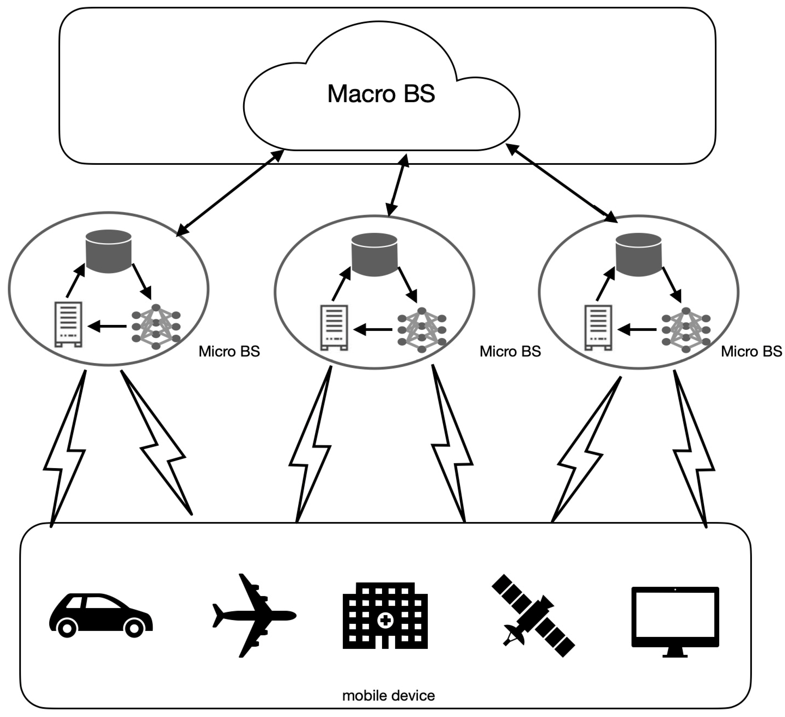
3.1. Network Architecture

In this paper, we consider a simple three-layer edge cloud computing model for multi-user MEC, as shown in Figure 1. The first layer is the IoT layer, which consists of a set of mobile devices. After the user decides the request offloading and computational resource scheduling, the IoT layer sends the request from mobile devices to the second edge layer or the third cloud layer. The edge layer is closer to the IoT layer and consists of a set of miniature base stations with edge servers. The cloud layer is further away from the IoT layer and consists of a macro base station with one deep cloud for processing large amounts of data and storing them for future use.
We assume that there is one macro base station with a cloud server, n micro base stations (BSs) with edge servers, and that the total number of mobile users is n. The locations and heights of all BSs are fixed. The average power consumption Pma and computational power Rma of the macro base station are two times the average power consumption Pmi and computational power Rmi of the micro base station, respectively. The maximum transmission power of a mobile user is Pmax. Each mobile user u generates one computational request at a time, and the request includes Qu = <Wq, Sg, Prg, Tgq, Tbq>, where Wq represents the workload of request q, i.e., the amount of computation required to fulfill the request, and Sg represents the size of the request input data. We use Prg to denote the request priority that represents the importance of different requests. Tgq and Tbq are the desirable latency threshold and tolerable latency threshold, respectively. The average delay Tavg = (Tgq + Tbq)/2 for request q. The location of the mobile user is denoted by put and the location of the base station is denoted by pnt.

3.2. Definition of JRORS

The JRORS problem is integrated as a system welfare maximization problem, and the goodness of solutions to the resource offloading and computational resource scheduling problems is summarized as the system welfare (W). In order to optimize the system efficiency, W takes into account the request response time, edge system utility, edge system cost, and extra cost. Moreover, to improve QoS, we add application completion and cloud server pricing to the considerations. We formulate the PA problem as in Equations (1) and (2). Request q is obtained from all request queues Q , and the base station n belongs to all BSs. Where x q n denotes an indication whether request q is assigned to the base station or not, where 0 denotes assignment to a macro base station and 1 denotes assignment to a micro base station. R n represents the computing power of base station n , and R q n represents the computing resources allocated by base station n to request q , k q denotes the edge system utility, c q denotes the edge system cost of processing request q , and e q denotes the additional cost of offloading request q to the macro base station. In Equation (3), c _ r denotes the computation of the application completion rate, and in Equation (4), c o s t denotes the server pricing, which consists of the edge server pricing c o s t M i and the cloud server pricing c o s t M a . λ 1 and λ 2 are the weights of the program completion rate and the server pricing.
  s . t .   n N max W x q n 1   , q Q x q n { 0 , 1 }   q Q , n N   q Q R q n R n   n N R q n > 0 ,   q Q , n N .
W = n N q Q [ x q n ( k q c q ) ( 1 x q n ) e q ] + λ 1 × c _ r λ 2 × c o s t
c _ r = n N x q n c o s t
c o s t = c o s t M a + c o s t M i

3.3. Definition of PA

The PA problem is a key issue in IoT that involves rationally distributing the limited transmission power to different users to maximize the system performance. To minimize the energy E consumed by the entire system in transmitting data, we formulate the PA problem as Equation (5). Where, p un   ( t ) represents the transmission power from mobile user u to base station n, and this is limited by the upper power limit p max .
min E = n N u U E u tra   ( t )
E u tra ( t ) = p u n ( t ) · t up q s . t .   0 p un   ( t ) p max   n N , u U
where E u tra   ( t ) is the transmission energy consumption for each data offload from mobile user u to the BS n, described by Equation (6). The constraint on p un   ( t ) guarantees the transmission power of each mobile user. t up q represents the uplink transmission time from request q to base station n.
The solution of the power allocation problem can help optimize network performance and improve communication quality and energy efficiency. However, due to the complex channel characteristics, interference, and power constraints involved, the problem is a nonconvex, nonlinear, and multidimensional optimization problem that requires the use of appropriate optimization algorithms to find the optimal solution.

4. Proposed Approach

This section describes the detailed construction process of the two proposed algorithms AGDOA and BSSA.

4.1. BSSA Algorithm

4.1.1. SSA Model

SSA is an optimization algorithm inspired by the migratory and collaborative behaviors of a salp swarm in nature, and solves optimization problems by simulating these behaviors. After initializing the population, each bottlenose sea squirt is evaluated for fitness and ranked in the chain according to its fitness value. The top ranked bottlenose sea squirts in the chain are called leaders, and the remaining part are called followers [33]. They update their positions according to different principles, and the position x j i of the leader is updated using Equation (7).
x j i = { F j + c 1 ( ( u b j l b j ) · c 2 + l b j ) c 3 0 F j c 1 ( ( u b j l b j ) · c 2 + l b j ) c 3 < 0 ,
where F j is the position of the food source in the jth dimension; u b j is the upper bound of the jth dimension; l b j is the lower bound of the jth dimension; and c 1 , c 2 , and c 3 are random numbers.
The updating of the follower’s position is borrowed from the idea of Newtonian motion and is represented by Equation (8).
x j i = 1 2 a t 2 + v 0 t , a = v final   v 0 , v = x x 0 t .
where i ≥ 2 denotes the position of the ith follower bottle sea squirt in the jth dimension, and t is the time. v stands for velocity, where v 0 is the initial velocity, v final   is the final velocity, x and x 0 represent the current and initial locations, respectively. The pseudo-code for SSA is shown in Algorithm 1.
Algorithm 1: Salp Swarm Algorithm (SSA)
  Input: ub, lb
  Output: fitness
 1: xi ←initial salp population considering ub and lb
 2: function SSA()
 3: while end condition is not satisfied do
 4:    Calculate the fitness of each search agent (salp)
 5:      Set F as the food source
 6:      for each salp ( x i ) do
 7:        if The salp population is in the top half then
 8:          Update the position of the leading salp using Equation (7)
 9:        else
 10:         Update the position of the follower salp using Equation (8)
 11:       end if
 12:     end for
 13:    end while
 14:   return F
 15: end function
The movement and interaction of virtual sheaths in the search space give SSA a strong global search capability; meanwhile, the diversity characteristics of SSA make it perform well in dealing with multi-peak optimization problems, which is suitable for searching for the optimal workload allocation scheme.

4.1.2. Proposed BSSA Algorithm

SSA has wide applicability and can solve continuous or discrete optimization problems. The load allocation problem we are going to solve is also a discrete optimization problem, this problem requires finding a set of binary schemes for power allocation that maximizes the fairness of the whole system. When we decide to allocate or not to allocate a certain workload to a particular base station, this is represented by 1 or 0. If this decision variable is represented using binary, it can be better adapted to the characteristics of the problem and the problem complexity can be reduced, to improve the performance of the algorithm. Therefore, we introduce binary coding into SSA, as in BSSA.
The pseudo-code for the key parts of the BSSA algorithm is reported in Algorithm 2. The fval_BSSA is the optimal fitness value, i.e., the maximum welfare value for searching for load assignments using BSSA. BSSA uses the pseudo-code of the binary modified procedure for Algorithm 2.
Algorithm 2: BSSA
  Input: user_profile , na_min, na_max, max_lter, N
  Output: fval_BSSA
  Initialize parameters
    1: lb ← 0
    2: ub ← 1
    3: thres ← 0.5
    4: max_lter ← 600
    5: convlter ← 0
    6: dim ← length(user_profile)
    7: Q ← 0.7
    8: beta1 ← −2 + 4 × rand()
    9: beta2 ← −1 + 2 × rand()
    10: nalni ← 2
    11: na ← round(na_min + (na_max − na_min) × rand())
    12: while t <= max_lter do
    13:   for i ← 1 to N do
    14:     Calculate fitness fit(i) using JRORS function
    15:     Negate fit(i)
    16:     if fit(i) > fitF then
    17:       Set Xf = X(i,:) and fitF = fit(i)
    18:       End if
    19:   End for
    20:   Update X as Leader Salp or Follower Salp
    21:     Set curve(t) ← fitF
    22:      Increment t
    23:End while
    24: Convert binary positions to feature subsets
    25: Determine Sf, Nf based on Xf
    26: Calculate sFeat from user_profile and Sf
    27: return fval_BSSA ← fitF
According to Algorithm 2, the detailed steps of BSSA are as follows:
  • Initialize the population. Within the upper bound 1 and lower bound 0 of the search space, a salp swarm of size N × D whose position is binary is randomly initialized;
  • Calculate the initial fitness. According to Equation (1), the fitness values of N salps in the JRORS problem are calculated;
  • Choose food. The salp swarm is sorted according to the fitness value, and the position of the salp swarm with the best fitness in the first place is set as the current food position;
  • Choose leaders and followers. After the food location is selected, there are N − 1 remaining salps in the group, and according to the ranking of the salp groups, the salps in the first half are regarded as leaders and the rest as followers;
  • Location update. First, the position of the leader is updated according to Equation (7), and then the position of the follower is updated according to Equation (8);
  • Calculate the fitness. Compute the fitness of the updated population. The updated fitness value of each individual salp sheath is compared with the fitness value of the current food. If the fitness value of the updated salp sheath is higher than that of the food, the salp sheath position with the higher fitness value is taken as the new food position;
  • Repeat steps 4–6 until a certain number of iterations is reached, and the current food position is output as the estimated position of the target.

4.2. AGDOA Algorithm

4.2.1. DOA Model

The DOA is a group intelligence optimization algorithm inspired by the hunting strategy of the Australian dingo, and the algorithm implements three strategies based on the dingo’s social behaviors, which are group hunting, individual attack, and scavenging behavior. Meanwhile, considering the species endangerment of the Australian dingo, a survival probability strategy is added to this algorithm [34].
The trajectory of the group hunting is modeled by Equation (9):
x i ( t + 1 ) = β 1 k = 1 n a [ φ k ( t ) x i ( t ) ] n a x * ( t ) ,
The trajectories of individual attacks are modeled by Equation (10):
x i ( t + 1 ) = x * ( t ) + β 1 e β 2 [ x r 1 ( t ) x i ( t ) ] ,
The trajectory of the sweeping behavior is simulated by Equation (11):
x i ( t + 1 ) = 1 2 [ e β 2 x r 1 ( t ) ( 1 ) σ x i ( t ) ] ,
When in low survival, Equation (12) will be used to update the position:
x i ( t ) = x * ( t ) + 1 2 [ x r 1 ( t ) ( 1 ) σ x r 2 ( t ) ] ,
Table 1 summarizes the key notations of DOA. The dingo in the algorithm chooses the strategy for updating the position based on a specific probability. The DOA relies on its strategy for updating the diversity of strategies to have an advantage in solving NP-hard puzzles to find a globally optimal solution.

4.2.2. DOA Considering Greedy Strategies

A population intelligence optimization algorithm’s optimization performance is, in part, determined by how well it is initialized. The initialization of the population position of the DOA is generated in a random way. It is quite challenging to find the optimal solution around the feasible solution when the objective value is modest in relation to the data and the first solution chosen at random is considerably far from the ideal solution. The usual methods of optimization initialization are greedy algorithm initialization [35], sampling initialization [36], and heuristic rules initialization [37]. In practice, sampling initialization and heuristic rules initialization are often used in combination. Sampling initialization can provide diversity and help the algorithm better explore the search space, while heuristic rules initialization can provide better quality initial solutions, which helps accelerate the convergence of the algorithm and improves the quality of the final solution. The greedy algorithm constructs the solution step by step in a locally optimal way and tries to satisfy the constraints as much as possible. This method can obtain a better initial solution. We will use the greedy principle to optimize the initialization process of DOA. The pseudocode for the greedy strategy is shown in Algorithm 3.
Algorithm 3: Greedy Initialization
  Input: alloted_bs, U, punt
  Output: initial_profile
  Initialize parameters:
    1: initial_profile ← Create a matrix of size (|U| × |n|) with initial values as pmax
    2: function greedy_initialization(alloted_bs, U, punt)
    3:  for each user u in U do
    4:    Get the current allocated base station index n for user u
    5:    Set initial_profile[u,n] to punt[u,n]
    6:  end for
    7:  return initial_profile
    8: end function
This greedy initialization procedure receives some input parameters: alloted_bs, gunt, U, punt, and pmax. These parameters denote the assigned base station for each user, the channel power gain, the set of mobile users, the transmission power, and the maximum transmission power, respectively. The allocation assigns the user power allocation scheme to the nearest base station, while the initial power of the other base stations remains unchanged. Finally, the initial power allocation scheme for each user to each base station is returned.
The greedy algorithm, as a concise method for optimizing the initial value, can provide an initial solution closer to the global optimal solution for the PA problem, reduce the number of iterations of the DOA, speed up the convergence of the algorithm, and improve the search performance of the DOA on the PA problem.

4.2.3. Proposed AGDOA Algorithm

The PA problem is a complex non-convex problem, and as it requires nonlinear computation, taking into account the data demand, channel gain, noise level, etc., this optimization method is more likely to find a local optimum. Therefore, in order to reduce the possibility of DOA falling into local optimality, we introduce the convergence speed adaptive adjustment mechanism.
We judge the convergence speed of the algorithm by monitoring the change in the optimal fitness, and then dynamically adjust the parameter na of the number of wild dogs involved in the attack strategy in DOA to balance the exploration and exploitation strategies of the algorithm. When the continuous change in the optimal fitness is small, this indicates that the algorithm may be converging, at which time, na is multiplied by 0.9 to reduce the number of dingoes participating in the attack, thus slowing down the search speed, with a view to better converging in the local search space; when the continuous change of the optimal fitness is large, na is multiplied by 1.1 to increase the number of dingoes participating in the attack, thus speeding up the search speed, with a view to better search the global space.
The pseudo-code for the adaptive tuning scheme is reported in Algorithm 4. Where tol is the convergence criterion, max_counter is the maximum number of convergence counts, and na_min and na_max are the minimum and maximum values of na, respectively. In each iteration, the optimal fitness change diff_vMin is computed, based on which the value of na is adaptively adjusted.
Algorithm 4: Adjust Parameters Adaptively
  Input: Max_iter, Curve, tol, max_counter, vMin
  Output: Adjusted value of na based on adaptive mechanism
  1: tol_counter ← 0
  2: for t ← 1 to Max_iter do
  3:  Calculate vMin for current iteration
  4:  if t > 1 then
  5:      Calculate diff_vMin = abs(Curve(t) − Curve(t + 1))
  6:   if diff_vMin < tol then
  7:    Increase tol_counter by 1
  8:  else
  9:    Reset tol_counter to 0
  10:   if tol_counter >= max_counter then
  11:    Decrease na
  12:  else
  13:    Increase na
  14: end for
  15: return na
The pseudo-code for the key parts of the AGDOA algorithm is reported in Algorithm 5. SearchAgents_no is the number of search agents, Max_iter is the maximum number of iterations, fobj is the fitness function, positions is the initial individual position matrix, ub and lb are the upper and lower bounds of the solution space, and vMin is the optimal fitness value. In order to facilitate an intuitive understanding, Figure 2 shows an algorithm flow chart. Figure 2 shows the process of the DOA algorithm integrating the greedy strategy to obtain the initial solution and dynamically changing the parameter adaptive strategy according to the degree of convergence, thus forming the operation flow of the AGDOA algorithm.
Algorithm 5: AGDOA
Input: Max_iter, Curve, conver_tol, conver_counter, na_min, na_max
Output: vMin
Initialize parameters
  1: threshold ← 0.005
  2: converged ← false
  3: consecutive_iterations ← 10
  4: iteration_count ← 0
  5: convlter ← 0
  6: P ← 0.5
  7: Q ← 0.7
  8: beta1 ← −2 + 4 × rand()
  9: beta2 ← −1 + 2 × rand()
  10: nalni ← 2
  11: na ← round(na_min + (na_max − na_min) × rand())
  12: Positions ← initialize from Algorithm 3
  13: for each position i in Positions do
  14:   Calculate Fitness(i)
  15: end for
  16: for each iteration t from 1 to Max_iter do
  17:   for each agent r from 1 to SearchAgent_no do
  18:     sumatory ← 0
  19:     if random number() < P then
  20:       Calculate sumatory using Attack function
  21:       if random number() < Q then
  22:         Update Agent position using strategy for group attack by Equation (9)
  23:       else
  24:         Update agent position using strategy for persecution by Equation (10)
  25:       end if
  26:     else
  27:       Update agent position using strategy for scavenging by Equation (11)
  28:     end if
  29:     if survival rate is below 0.3 then
  30:       Execute survival process to update agent position by Equation (12)
  31:     end if
  32:     Calculate Fnew
  33:     if Fnew <= Fitness(r) then
  34:       Update agent position and fitness value
  35:     end if
  36:     if Fnew <= vMin then
  37:       Count and update convlter
  38:       Update theBestVct and vMin
  39:     end if
  40:   end for
  41:   Update na by Algorithm 4
  42: end for
  43: return vMin
According to Algorithm 5 and Figure 2, the specific steps of AGDOA are as follows:
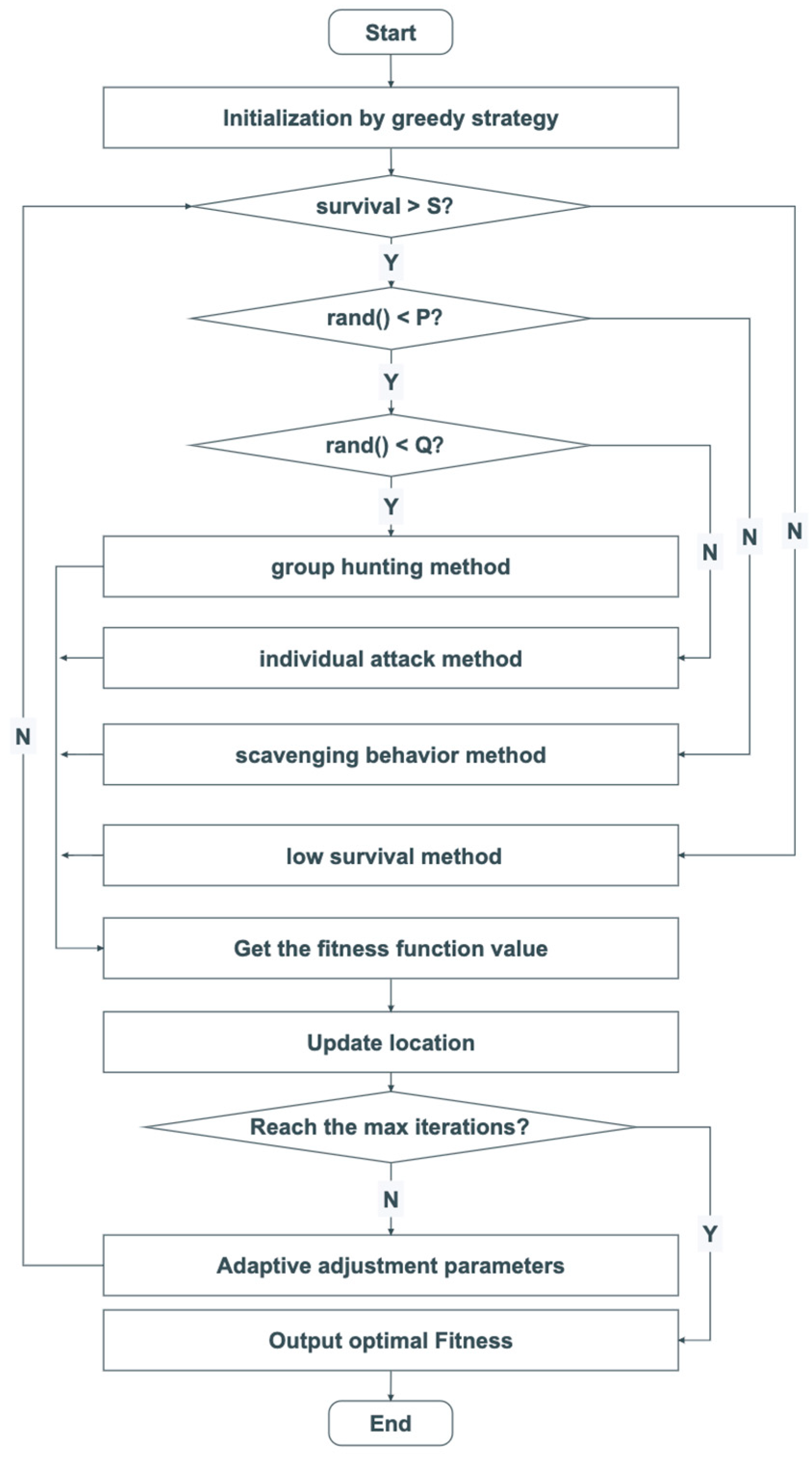
  • Use Algorithm 3 to initialize the dingo population position through the greedy strategy;
  • Calculate the survival probability;
  • If the survival probability is greater than the set point, jump to step 4, otherwise jump to step 9;
  • If the random value is less than P, jump to step 5, otherwise jump to step 8;
  • If the random value is less than Q, jump to step 6, otherwise jump to step 7;
  • Perform a group attack according to Equation (9) to update the agent location;
  • Perform individual persecution according to Equation (10) to update the agent location;
  • Perform the clearance strategy according to Equation (11) to update the agent location;
  • Update the position of the group with low survival rate according to Equation (12);
  • Update the fitness value and the agent location;
  • If the maximum number of iterations is not reached, update the adaptive parameters according to Algorithm 4 and repeat steps 2–10, otherwise output the optimal fitness;

5. Experimental Setup

In this section, computer simulations were used to evaluate the performance of the proposed AGDOA algorithm and BSSA algorithm. The performance of the proposed algorithms was evaluated under different system parameters in comparison with the existing schemes.

5.1. Simulation Settings

To evaluate the performance of the algorithms, we ran the AGDOA algorithm and the BSSA algorithm using MATLAB R-2021a. The simulation device PC was configured with 16 GB of memory, and a 2.6 GHz Intel Core i7. The simulation parameters are shown in Table 2.

5.2. Comparative Experiments

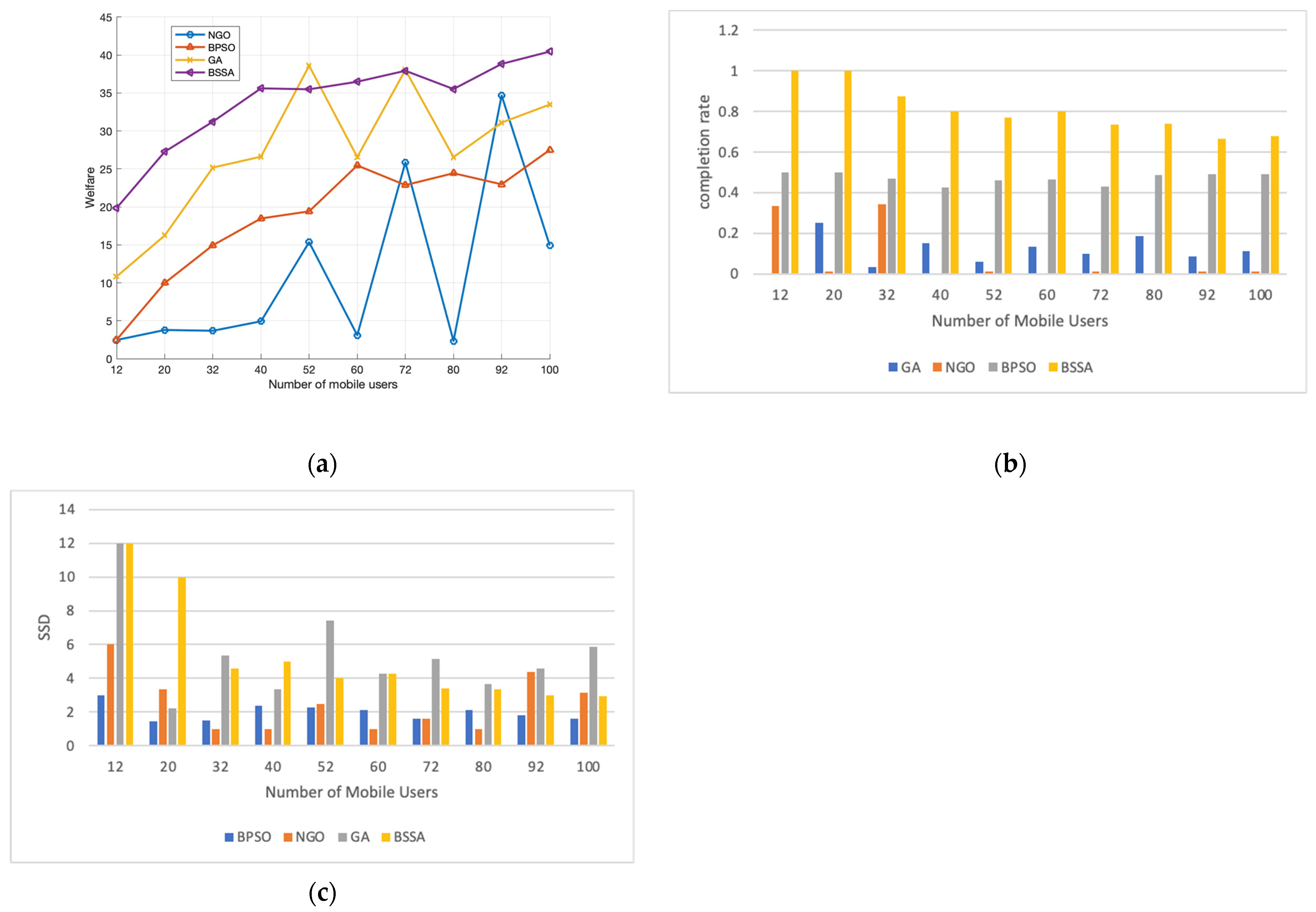
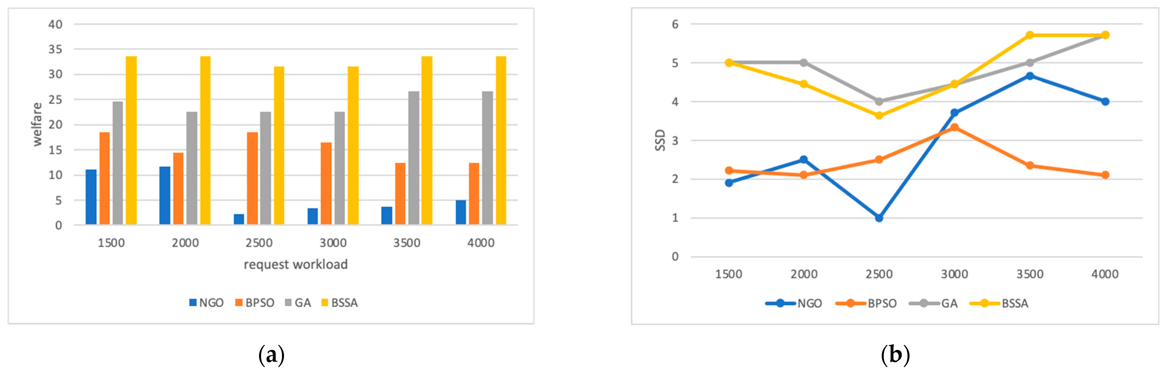
5.2.1. Comparative Experiments of BSSA

We compared the performance of the BSSA algorithm with the following methods:
  • Northern Goshawk Algorithm (NGO): NGO is a relatively new algorithm that has the advantage of diverse search strategies that may help to better explore the solution space [13];
  • Genetic Algorithm (GA): The GA performs well in dealing with discrete problems and can effectively represent and manipulate discrete decision variables through the use of binary or integer coding [38].
  • Binary Particle Swarm Optimization Algorithm (BPSO): BPSO is suitable for discrete optimization problems and it can represent the decision variables of the problem in binary [39].

5.2.2. Comparative Experiments with AGDOA

We compared the performance of the AGDOA algorithm with the following methods:
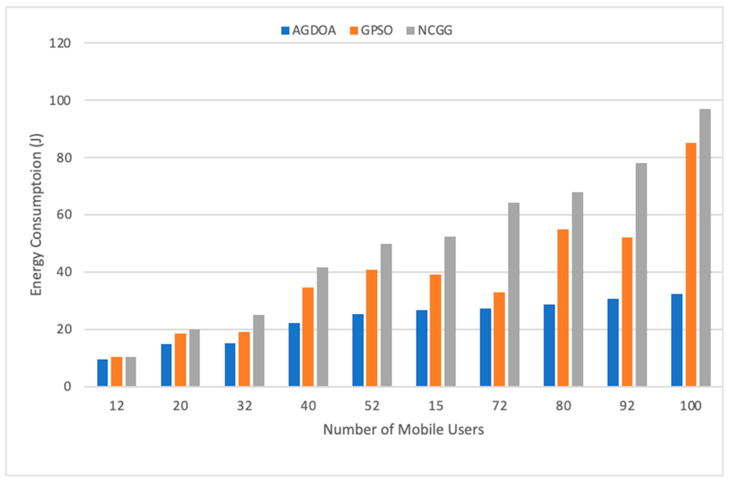
  • Greedy Particle Swarm Optimization (GPSO): The PSO application has advantages for multivariate problems and is suitable for solving PA problems involving power allocation decisions among multiple mobile users and multiple base stations. Meanwhile, the initialization of the particle swarm was optimized using a greedy strategy to obtain GPSO [40];
  • Simulated Annealing PA: Simulated annealing (SA) is suitable for complex problems and can effectively solve discrete NP-hard problems [41];
  • Subgradient-based non-cooperative game model (NCGG): the NCGG algorithm is usually used to solve the problem of optimal decision making for multiple participants in a game, and is suitable for optimizing the multi-user PA problem [42].

5.3. Performance Metrics

5.3.1. Convergence Speed

To evaluate the convergence speed of the algorithm, we used the successive absolute change magnitude to determine whether the change in the objective function value was stabilizing or not. The absolute change in the objective function value between adjacent iterations was calculated, i.e., r = |f(i) − f(i − 1)|, and the magnitude threshold e was set to 0.005. The algorithm was judged to have stabilized when the absolute change in the magnitude of r was less than the magnitude threshold e. The algorithm was also evaluated to prevent the algorithm from falling into a local optimum. At the same time, in order to prevent the algorithm from being misjudged as converging when it fell into a local optimum, when the algorithm’s r was less than e for 10 consecutive iterations, we considered that the algorithm had reached convergence, and the mobile user was considered to have found the best solution.

5.3.2. System Response Rate

To evaluate the efficiency and performance of the system, we considered the number of tasks completed within a tolerable delay time for the request versus the total number of requested tasks, defined as the system response rate.

5.3.3. Scheduling Dominance Degree (SDD)

In order to evaluate the task completion degree, i.e., the fairness, we used SSD in the performance evaluation. SSD is a metric used to evaluate the fairness of a task resource allocation scheme, and there is an inverse relationship between it and the fairness metric. SSD is expressed by Equation (13). F is the fairness metric, and r i indicates the resource allocation for user i . In general, a larger SSD value indicates better fairness, while a smaller SSD value indicates worse fairness. We calculated SSD based on the fairness indicator Jain’s fairness index.
S S D = 1 F F = ( i = 1 N r i ) 2   N × i = 1 N r i 2     s . t .           r i { 0 , 1 }

6. Performance Evaluation and Analysis

In this section, we performed a simulation and analyzed the results of the experiment.

6.1. Performance of BSSA

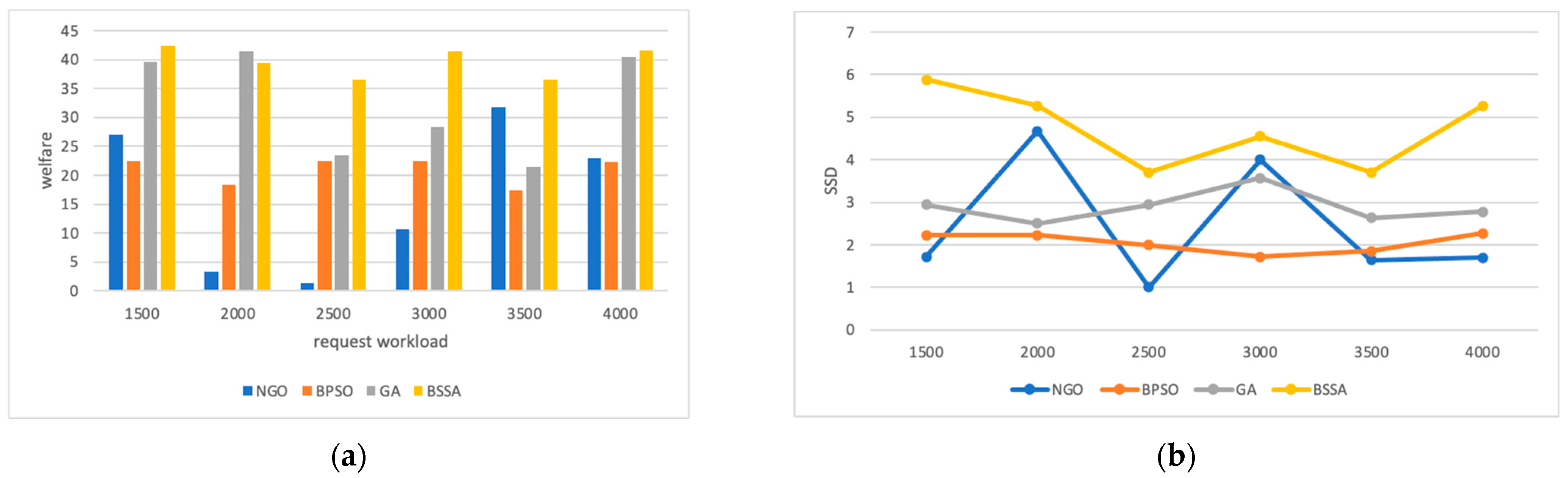
6.1.1. Impact of the Number of Mobile Users

In this section, we set the base station with the same computational power, i.e., Rn = 70 GHz, and all mobile user offloading tasks were configured with the same request conditions, wq = 1500 (Megacycles), lg = 700 KB, Tgq = 0.5 (s), Tbg = 0.65 (s). We output the welfare of the system after it had run, in order to assess the effectiveness of the solution to the resource offloading and computational resource scheduling problem; that is, the performance of the fitness function JRORS, under the influence of various numbers of mobile users. To assess the efficiency and performance of the system, we took into account the system response rate, and to assess the fairness of the system, we took into account the SSD. NGO, BPSO, GA, and BSSA are all suitable algorithms for solving discrete optimization problems.
From Figure 3a, we can observe that NGO and GA showed an overall increasing trend in welfare with the increase in the number of mobile users, but there was oscillating instability. BPSO and BSSA showed a flat increase in welfare with the increase in the number of mobile users. This was because, as the number of users increased, more requests may be generated in the system, and when these requests are reasonably handled and satisfied, the total utility of the system may increase. In terms of welfare performance, NGO performed poorly, which means that NGO cannot achieve good results for the JRORS problem. BSSA had a larger welfare with a different number of mobile users, which means that BSSA can obtain a better solution when multiple factors are considered for scheduling computational resources. Compared to GA, the proposed BSSA improved by about 100% for welfare when the number of mobile users was 12 and by about 20% when the number of mobile users was 100. The complexity of the problem grows exponentially as the number of users increases. Both BSSA and GA needed to search the large-scale solution space, and hence the size of the BSSA boost became smaller. However, due to the addition of binary, the complexity of BSSA decreased on the discrete problem JRORS, so it was easier to search for a better resource allocation scheme for welfare. Figure 3b illustrates that BPSO and BSSA had a larger system responsiveness, and BPSO’s system responsiveness did not change much for different numbers of mobile users. Compared with BPSO, BSSA had almost a 1x improvement in the corresponding rate when the number of mobile users was 12. BSSA’s response rate naturally decreased slightly with the increase in the number of mobile users, due to the consequent increase in the search space and the complexity of the problem, but it still managed to maintain a higher response rate, which also reflects the scalability of BSSA. Compared with BPSO, at a mobile user number of 100, BSSA improved in its response rate by about 40%, which was due to the fact that the search strategy of BSSA is more suitable for the JRORS problem. From Figure 3c, it can be seen that the SSD of BSSA and GA was larger in most of the cases in the comparison experiments, which proved that the fairness of BSSA was better. Moreover, the SSD of BSSA decreased smoothly with the increase in the number of mobile users, which proved that BSSA had the best fairness when the number of mobile users was small. This is due to the fact that competition among a large number of users may lead to more competitive resource allocation. This may result in certain users always having a dominant position, while other users are unable to obtain a fair share, thus reducing the fairness. At the same time, since the SSA algorithm has the unique advantage that the group tends to move in the direction of greater comfort, this leads to a smooth, progressive search process that avoids drastic fluctuations, and the experiments yielded smooth changes for each of the performance metrics as the number of mobile users was varied.

6.1.2. Impact of Request Workloads

In this section, we set the base station with the same computational power, i.e., Rn = 70 GHz, and all mobile users had offloading tasks configured with the same request conditions lg = 700 KB, Tgq = 0.5 (s), Tbg = 0.65 (s), except for the workload wq being set to a different request q. The performance of the BSSA was evaluated at wq = 1500, 2000, 2500.
From Figure 4a, it can be observed that the system welfare decreased as the request workload increased. When the workload increased from 1500 to 2000, welfare decreased by about 4% on average; when the workload increased from 2000 to 2500, the welfare decreased by about 2% on average. This is due to the fact that when the computational task requests from the BS exceed the scheduling load that the base station can handle, it becomes under-resourced and reduces the system welfare value. Figure 4b shows that when the number of mobile users is small, different request workloads have essentially no effect on the SSD. When the number of mobile users was high, the SSD decreased by 3% on average as the request workload increased; i.e., an appropriate request workload had a benign effect on the system fairness. At high loads, the system’s resources became saturated and resource allocation delays increased, leading to a decrease in fairness when the system performed offloading tasks.

6.1.3. Impact of Request Workload Configuration

In this section, different workload requests (wq) and different amounts of work input data requests (Iq) were configured, to evaluate the performance of the BSSA and compare the experiments with other optimization algorithms. The following figure shows the system welfare and SSD used for evaluating the system with different wq when the number of mobile users (u) was 40 and 100, respectively.
From Figure 5a,b, it can be observed that the welfare of the BSSA was consistently higher than other methods at different wq values when the number of mobile users was small. When the number of mobile users was 40, the proposed BSSA improved the welfare of GA by 36.2% on average. For SSD, the values of BSSA and GA were significantly larger than the other methods, and BSSA was inferior to GA for smaller wq. This implied that, at this point, BSSA sacrificed part of the system fairness to maintain a higher system welfare during the optimization process. From Figure 6a,b, it can be seen that the welfare of BSSA and GA became larger as the number of mobile users u increased, and the proposed BSSA improved the welfare of GA by only 29.4% on average, while at this time, the SSD of BSSA had a significant advantage at different wq. Meanwhile, the SSD of BSSA showed an overall decreasing trend with the increase in wq. Obviously, as the number of mobile users u increased with the increase in wq, more and more tasks could not be completed in time, resulting in a decrease in the fairness of the system. Similarly, as shown in Figure 7a,b, BSSA consistently performed the best in terms of system welfare for different amounts of Iq. The proposed BSSA’s welfare improved by 35.7% and 16.0% on average under the conditions of 40 and 80 mobile subscribers, respectively. Thus, we can say that BSSA showed the best performance for the system welfare problem, even under different request work configurations.

6.2. Performance of AGDOA

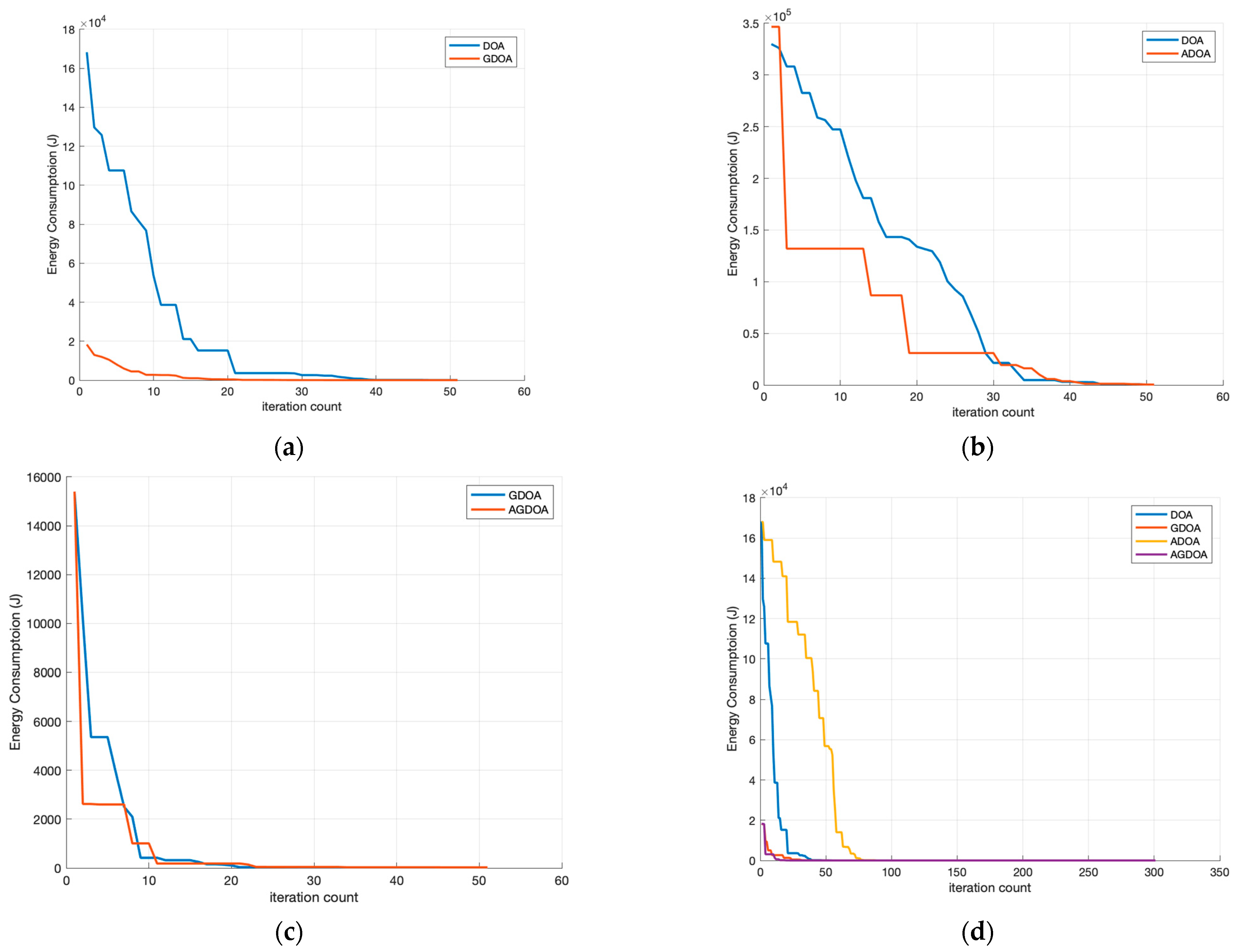
6.2.1. Ablation Experiments

The following figure shows a comparison of the energy consumption of DOA, GDOA, ADOA, and AGDOA for the same number of mobile users, number of server base stations, and maximum power. We can see from Figure 8a that a using greedy strategy to optimize the initial value of DOA, the initial energy consumption was significantly reduced, which was conducive to faster convergence. We can see from Figure 8b that after making the parameter na adaptive change, the iteration frequency was perturbed, and the speed of each descent became faster, which helped to prevent the DOA from falling into a local optimum. We can see from Figure 8c that after using the greedy strategy to optimize the initialization process of DOA and making the parameter na change adaptively, the optimized DOA algorithm obtained a better initial value, while descending faster. The overall ablation experiment results in Figure 8d showed that the greedy algorithm and the adaptive strategy improved the DOA significantly, bringing about a lower initial value, speeding up the iteration speed, and preventing from falling into a local optimum.
In order to assess the convergence properties of the AGDOA in the ablation experiments, we used the number of iterations required for the algorithm to reach the converged state as the convergence rate for comparison. The number of convergence iterations for the different numbers of mobile users in DOA, GDOA, ADOA, and AGDOA are listed in Table 3. As shown in Table 3, the greedy strategy contributed more to the convergence speed of DOA than parameter adaptation, and AGDOA exhibited the maximum convergence speed in the ablation experiments. In terms of the quantity of iterations required to obtain convergence, AGDOA was at least 11.2% faster than GDOA. This was the result of the joint involvement of the greedy strategy and the adaptive tuning parameter strategy.

6.2.2. Energy Consumption vs. Number of Mobile Devices

We set the maximum transmission power Pmax for mobile users uniformly at 5 W. Figure 9 shows a comparison of the energy consumption of the proposed AGDOA compared to GPSO and NCGG for different numbers of mobile users. It is clear that the energy consumption increased as the number of mobile users increased. The energy consumption of AGDOA was always smaller than that of GPSO and NCGG for different numbers of mobile users, and the gap between the energy consumption of AGDOA and the comparison algorithms gradually increased as the number of mobile users increased. The proposed AGDOA increased the degree of improvement in energy consumption from 8.3% to 163.9% compared to the GPSO. This suggests that the AGDOA outperforms GPSO and NCGG in the PA problem and performs better when there are a lot of mobile users.

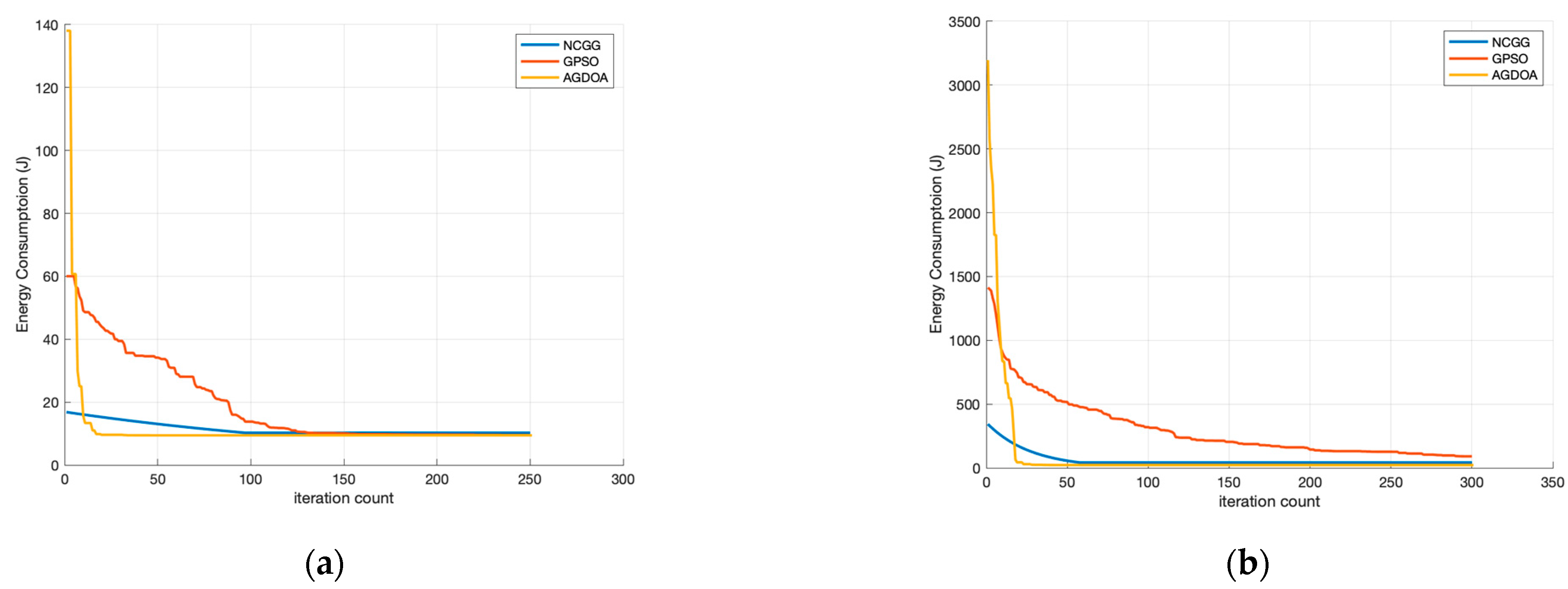
6.2.3. Convergence Properties of AGDOA

To determine the convergence characteristics of AGDOA, we similarly compared the number of iterations required for the algorithms to reach a converged state. The convergence characteristics of AGDOA were evaluated by setting the maximum transmission power Pmax of mobile users to 5 w with the same number of mobile users u and the number of base stations of edge servers n. The convergence characteristics of AGDOA were evaluated by setting the maximum transmission power Pmax of mobile users to 5 w. As shown in Figure 10a, when u was 12 and n was 3, AGDOA needed only 61 iterations to converge, while NCGG and GPSO needed 107 and 200 iterations, respectively; as shown in Figure 10b, when u was 40 and n is 10, AGDOA needed only 61 iterations to converge, while NCGG and GPSO needed 107 and 200 iterations, respectively; AGDOA required only 72 iterations to converge, while NCGG and GPSO required 168 and 229 iterations, respectively. As can be seen from Figure 10a,b below, AGDOA reached convergence in fewer iterations, even with larger initial values. This indicates that our proposed AGDOA has good convergence properties.

7. Conclusions

In this paper, we studied a MEC network consisting of a macro BS, a set of micro BSs, and a large number of mobile users, aiming to solve two main problems in task scheduling with federated learning in a network. For the JRORS dual decision problem, we incorporated the consideration of server pricing and task completion factors to improve user-friendliness and fairness. Meanwhile, a BSSA was proposed to solve this problem based on the discrete nature of JRORS, to reduce the problem complexity. Then, for the PA problem, an AGDOA was proposed to find the optimal power allocation scheme.
The simulation results validated the proposed algorithm, in which the BSSA maintained a good performance for welfare, response rate, and SSD for the JRORS problem. Compared with the heuristic algorithms NGO, BPSO, and GA, the proposed BSSA could find better solutions and obtained a higher welfare under different numbers of mobile users, workloads, and input data amounts. This was due to the addition of binaries, which reduced the complexity of the BSSA on discrete problems such as JRORS. In addition, the BSSA had a higher system response rate, and the number of tasks completed within a tolerable delay time of the request was more than the total number of requested tasks. Moreover, compared with the other heuristics compared, the BSSA paid more attention to fairness in task offloading.
In addition, compared with the other algorithms, on the PA problem, each improved module of AGDOA showed a significant improvement in convergence speed and initial performance over the DOA. Compared with the optimization algorithms GPSO and NCGG, the energy consumption of the AGDOA was significantly lower under different numbers of mobile users. At the same time, the AGDOA could reach a convergence state in fewer iterations for different numbers of mobile devices.
In the future, we will conduct experiments using real data, make improvements based on real applications, and apply the proposed algorithms to real applications to improve the MEC scheduling efficiency and the comprehensive level of QoS.

Author Contributions

Conceptualization, W.C.; methodology, W.C.; software, F.D.; validation, F.D.; formal analysis, F.D.; investigation, F.D.; resources, W.C.; data curation, W.C.; writing—original draft preparation, F.D. and W.C.; writing—review and editing, F.D. and W.C.; visualization, F.D.; supervision, W.C.; project administration, F.D. and W.C.; funding acquisition, W.C. All authors have read and agreed to the published version of the manuscript.

Funding

This research was funded by Science and Technology Planning Project of Guangdong Province, grant number (2019B010116001,2016B010124012).

Data Availability Statement

Not applicable.

Conflicts of Interest

The authors declare no conflict of interest.

References

  1. Du, X.; Chen, X.; Lu, Z.; Duan, Q.; Wang, Y.; Wu, J.; Hung, P.C. A Blockchain-Assisted Intelligent Edge Cooperation System for IoT Environments with Multi-Infrastructure Providers. IEEE Internet Things J. 2023, 1. [Google Scholar] [CrossRef]
  2. Cao, X.W.; Wang, F.; Xu, J.; Zhang, R.; Cui, S. Joint computation and communication cooperation for energy-efficient mobile edge computing. IEEE Internet Things J. 2019, 6, 4188–4200. [Google Scholar] [CrossRef]
  3. Kishor, A.; Chakarbarty, C. Task Offloading in Fog Computing for Using Smart Ant Colony Optimization. Wirel. Pers. Commun. 2022, 127, 1683–1704. [Google Scholar] [CrossRef]
  4. Thapa, C.; Chamikara, M.A.P.; Camtepe, S.A. Advancements of federated learning towards privacy preservation: From federated learning to split learning. In Federated Learning Systems: Towards Next-Generation AI; Springer: Berlin/Heidelberg, Germany, 2021; pp. 79–109. [Google Scholar]
  5. Ma, X.; Zhu, J.; Lin, Z.; Chen, S.; Qin, Y. A state-of-the-art survey on solving non-IID data in Federated Learning. Future Gener. Comput. Syst. 2022, 135, 244–258. [Google Scholar] [CrossRef]
  6. Nadembega, A.; Taleb, T.; Hafid, A. A destination prediction model based on historical data contextual knowledge and spatial conceptual maps. In Proceedings of the 2012 IEEE International Conference on Communications (ICC), Ottawa, ON, Canada, 10–15 June 2012; pp. 1416–1420. [Google Scholar]
  7. Hou, X.; Li, Y.; Chen, M.; Wu, D.; Jin, D.; Chen, S. Vehicular Fog Computing: A Viewpoint of Vehicles as the Infrastructures. IEEE Trans. Veh. Technol. 2016, 65, 3860–3873. [Google Scholar] [CrossRef]
  8. Duan, S.; Wang, D.; Ren, J.; Lyu, F.; Zhang, Y.; Wu, H.; Shen, X. Distributed Artificial Intelligence Empowered by End-Edge-Cloud Computing: A Survey. IEEE Commun. Surv. Tutorials 2022, 25, 591–624. [Google Scholar] [CrossRef]
  9. Du, X.; Tang, S.; Lu, Z.; Wet, J.; Gai, K.; Hung, P.C.K. A Novel Data Placement Strategy for Data-Sharing Scientific Workflows in Heterogeneous Edge-Cloud Computing Environments. In Proceedings of the 2020 IEEE International Conference on Web Services (ICWS), Beijing, China, 19–23 October 2020; pp. 498–507. [Google Scholar]
  10. Chen, M.; Hao, Y.; Li, Y.; Lai, C.F.; Wu, D. On the Computation Offloading at Ad Hoc Cloudlet: Architecture and Service Modeo. IEEE Commun. Mag. 2015, 53, 18–24. [Google Scholar] [CrossRef]
  11. Du, X.; Chen, X.; Lu, Z.; Duan, Q.; Wang, Y.; Wu, J. BIECS: A Blockchain-based Intelligent Edge Cooperation System for Latency-Sensitive Services. In Proceedings of the 2022 IEEE International Conference on Web Services (ICWS), Barcelona, Spain, 10–16 July 2022; pp. 367–372. [Google Scholar]
  12. Krishnan, M.; Yun, S.; Jung, Y.M. Enhanced clustering and ACO-based multiple mobile sinks for efficiency improvement of wireless sensor networks. Comput. Netw. 2019, 160, 33–40. [Google Scholar] [CrossRef]
  13. Hu, S.; Li, G. Dynamic Request Scheduling Optimization in Mobile Edge Computing for IoT Applications. IEEE Internet Things J. 2020, 7, 1426–1437. [Google Scholar] [CrossRef]
  14. Market Research Report by International Data Corporation. Available online: https://www.idc.com/getdoc.jsp?containerId=prUS50936423 (accessed on 20 June 2023).
  15. Yin, L.; Feng, J.; Xun, H.; Sun, Z.; Cheng, X. A Privacy-Preserving Federated Learning for Multiparty Data Sharing in Social IoTs. IEEE Trans. Netw. Sci. Eng. 2021, 8, 2706–2718. [Google Scholar] [CrossRef]
  16. Tran, T.X.; Pompili, D. Joint task offloading and resource allocation for multi-server mobile-edge computing networks. IEEE Trans. Veh. Technol. 2019, 68, 856–868. [Google Scholar] [CrossRef]
  17. Du, X.; Tang, S.; Lu, Z.; Gai, K.; Wu, J.; Hung, P.C. Scientific workflows in iot environments: A data placement strategy based on heterogeneous edge-cloud computing. ACM Trans. Manag. Inf. Syst. (TMIS) 2022, 13, 1–26. [Google Scholar] [CrossRef]
  18. Ra, M.R.; Sheth, A.; Mummert, L.; Pillai, P.; Wetherall, D.; Govindan, R. Odessa: Enabling Interactive Perception Applications on Mobile Devices. In Proceedings of the 9th International Conference on Mobile Systems, Applications, and Services, Bethesda, MD, USA, 28 June–1 July 2011. [Google Scholar]
  19. Chen, C.; Chang, Y.-C.; Chen, C.-H.; Lin, Y.-S.; Chen, J.-L.; Chang, Y.-Y. Cloud-fog computing for information-centric Internet-of-Things applications. In Proceedings of the 2017 International Conference on Applied System Innovation (ICASI), Sapporo, Japan, 13–17 May 2017; pp. 637–640. [Google Scholar]
  20. Chang, Z.; Zhou, Z.; Ristaniemi, T.; Niu, Z. Energy efficient optimization for computation offloading in fog computing system. In Proceedings of the GLOBECOM 2017–2017 IEEE Global Communications Conference, Singapore, 4–8 December 2017; pp. 1–6. [Google Scholar]
  21. Alazab, A.; Venkatraman, S.; Abawajy, J.; Alazab, M. An optimal transportation routing approach using GIS-based dynamic traffic flows. In Proceedings of the ICMTA 2010, Proceedings of the International Conference on Management Technology and Applications, Singapore, 10 September 2010; Research Publishing Services: Singapore, 2011; pp. 172–178. [Google Scholar]
  22. Pham, Q.V.; Mirjalili, S.; Kumar, N.; Alazab, M.; Hwang, W.J. Whale optimization algorithm with applications to resource allocation in wireless networks. IEEE Trans. Veh. Technol. 2020, 69, 4285–4297. [Google Scholar] [CrossRef]
  23. Abdi, S.; Motamedi, S.A.; Sharifian, S. Task scheduling using modified PSO algorithm in cloud computing environment. In Proceedings of the International Conference on Machine Learning, Electrical and Mechanical Engineering, Dubai, United Arab Emirates, 8–9 January 2014; Volume 4, pp. 8–12. [Google Scholar]
  24. Mao, Y.; Zhang, J.; Letaief, K.B. Dynamic computation offloading for mobile-edge computing with energy harvesting devices. IEEE J. Sel. Areas Commun. 2016, 34, 3590–3605. [Google Scholar] [CrossRef]
  25. Shojafar, M.; Cordeschi, N.; Baccarelli, E. Energy-efficient adaptive resource management for real-time vehicular cloud services. IEEE Trans. Cloud Comput. 2019, 7, 196–209. [Google Scholar] [CrossRef]
  26. Haxhibeqiri, J.; Van den Abeele, F.; Moerman, I.; Hoebeke, J. LoRa scalability: A simulation model based on interference measurements. Sensors 2017, 17, 1193. [Google Scholar] [CrossRef]
  27. Mikhaylov, K.; Petäjäjärvi, J.; Janhunen, J. On LoRaWAN scalability: Empirical evaluation of susceptibility to inter-network interference. In Proceedings of the 2017 European Conference on Networks and Communications (EuCNC), Oulu, Finland, 12–15 June 2017; pp. 1–6. [Google Scholar]
  28. Tang, S.; Du, X.; Lu, Z.; Gai, K.; Wu, J.; Hung, P.C.; Choo, K.K.R. Coordinate-based efficient indexing mechanism for intelligent IoT systems in heterogeneous edge computing. J. Parallel Distrib. Comput. 2022, 166, 45–56. [Google Scholar] [CrossRef]
  29. Rajab, H.; Cinkler, T.; Bouguera, T. IoT scheduling for higher throughput and lower transmission power. Wirel. Netw. 2021, 27, 1701–1714. [Google Scholar] [CrossRef]
  30. Rodrigues, T.K.; Suto, K.; Kato, N. Edge cloud server deployment with transmission power control through machine learning for 6G Internet of Things. IEEE Trans. Emerg. Top. Comput. 2019, 9, 2099–2108. [Google Scholar] [CrossRef]
  31. Vispute, S.D.; Vashisht, P. Energy-Efficient Task Scheduling in Fog Computing Based on Particle Swarm Optimization. SN Comput. Sci. 2023, 4, 391. [Google Scholar] [CrossRef]
  32. Xia, W.; Shen, L. Joint Resource Allocation at Edge Cloud Based on Ant Colony Optimization and Genetic Algorithm. Wirel. Pers. Commun. 2021, 117, 355–386. [Google Scholar] [CrossRef]
  33. Mirjalili, S.; Gandomi, A.H.; Mirjalili, S.Z.; Saremi, S.; Faris, H.; Mirjalili, S.M. Salp Swarm Algorithm: A bio-inspired optimizer for engineering design problems. Adv. Eng. Softw. 2017, 114, 163–191. [Google Scholar] [CrossRef]
  34. Peraza-Vázquez, H.; Peña-Delgado, A.F.; Echavarría-Castillo, G.; Morales-Cepeda, A.B.; Velasco-Álvarez, J.; Ruiz-Perez, F. A bio-inspired method for engineering design optimization inspired by dingoes hunting strategies. Math. Probl. Eng. 2021, 2021, 9107547. [Google Scholar] [CrossRef]
  35. Pan, G.; Li, K.; Ouyang, A.; Li, K. Hybrid immune algorithm based on greedy algorithm and delete-cross operator for solving TSP. Soft Comput. 2016, 20, 555–566. [Google Scholar] [CrossRef]
  36. de Perthuis de Laillevault, A.; Doerr, B.; Doerr, C. Money for nothing: Speeding up evolutionary algorithms through better initialization. In Proceedings of the 2015 Annual Conference on Genetic and Evolutionary Computation, Yangon, Myanmar, 26–28 August 2015; pp. 815–822. [Google Scholar]
  37. Guo, M.; Xin, B.; Chen, J.; Wang, Y. Multi-agent coalition formation by an efficient genetic algorithm with heuristic initialization and repair strategy. Swarm Evol. Comput. 2020, 55, 100686. [Google Scholar] [CrossRef]
  38. Das, S.; Idicula, S.M. Greedy search-binary PSO hybrid for biclustering gene expression data. Int. J. Comput. Appl. 2010, 2, 1–5. [Google Scholar] [CrossRef]
  39. Alrefaei, M.H.; Andradóttir, S. A simulated annealing algorithm with constant temperature for discrete stochastic optimization. Manag. Sci. 1999, 45, 748–764. [Google Scholar] [CrossRef]
  40. Dehghani, M.; Hubálovský, Š.; Trojovský, P. Northern goshawk optimization: A new swarm-based algorithm for solving optimization problems. IEEE Access 2021, 9, 162059–162080. [Google Scholar] [CrossRef]
  41. Mirjalili, S.; Mirjalili, S. Genetic algorithm. In Evolutionary Algorithms and Neural Networks: Theory and Applications; Springer: Berlin/Heidelberg, Germany, 2019; pp. 43–55. [Google Scholar]
  42. El-Maleh, A.H.; Sheikh, A.T.; Sait, S.M. Binary particle swarm optimization (BPSO) based state assignment for area minimization of sequential circuits. Appl. Soft Comput. 2013, 13, 4832–4840. [Google Scholar] [CrossRef]
Figure 1. A three-layer edge cloud computing model.
Futureinternet 15 00357 g001
Figure 2. AGDOA algorithm flow chart.
Futureinternet 15 00357 g002
Figure 3. (a) The overall variation in the welfare of each algorithm with different numbers of mobile users; (b) the overall results of the system response rate of each algorithm with different numbers of mobile users; (c) the overall results of the SSD of each algorithm with different numbers of mobile users.
Futureinternet 15 00357 g003
Figure 4. (a) The overall change in welfare for each algorithm when changing the request workload for different numbers of mobile users; (b) the overall results in SSD for each algorithm when changing the request workload for different numbers of mobile users.
Futureinternet 15 00357 g004
Figure 5. The result of the experiment under u = 40. (a) The overall welfare results for each algorithm at different wq; (b) the variation in SDD for each algorithm at different wq.
Futureinternet 15 00357 g005
Figure 6. The result of the experiment under u = 100. (a) The overall welfare results for each algorithm at different wq; (b) the variation in SDD for each algorithm at different wq.
Futureinternet 15 00357 g006
Figure 7. (a) The overall welfare results for each algorithm with different Iq in the u = 40 condition; (b) the overall welfare results for each algorithm with different Iq in the u = 80 condition.
Futureinternet 15 00357 g007
Figure 8. A direct comparison of the energy consumption results of the different algorithms as the number of iterations increased. (a) DOA versus GDOA; (b) DOA versus ADOA; (c) GDOA versus AGDOA; (d) DOA, GDOA, ADOA, AGDOA.
Futureinternet 15 00357 g008
Figure 9. The energy consumption of different algorithms with different numbers of mobile users.
Futureinternet 15 00357 g009
Figure 10. (a) Variation in energy consumption with the number of iterations when u = 12 and n = 3; (b) variation in energy consumption with the number of iterations when u = 40 and n = 10.
Futureinternet 15 00357 g010
Table 1. Key Notations of DOA.
SymbolDescription
x i ( t + 1 ) New location for dingoes
φ k ( t ) Subset of search agents
x i ( t ) Current search agent, i.e., subset of wild dogs being attacked
x * ( t ) Iteration of the best subset of dingoes so far
x r 1 ( t ) , x r 2 ( t ) Randomly selected r 1 , r 2 search agent, i.e., subset of dingoes, where r 1 i
SizePop Total size of the dingo population
σ Randomly generated binary numbers, σ ϵ { 0 , 1 }
β 1 , β 2 Randomly generated scale factor
r 1 , r 2 Random numbers generated from [1, maximum search agent size] with r 1 r 2 ; x r 1 ( t )
Table 2. Simulation Parameters.
ParameterValue
Number of Mobile Users u{12,20,32,40,52,60,72,80,92,100}
Number of Micro-BSs n{3,5,8,10,13,15,18,20,23,25}
The fixed bandwidth B20 (MHz)
The fixed height of BSs H10 (m)
Workload of request wq600–1000 (MHz)
Input data of request lq300–1500 (KB)
Ideal delay of request q Tgq0.5 ± 0.1 (s)
Tolerable delay of request q TbqTgq + [0.1,0.15] (s)
Maximum transmission power for mobile users Pmax5 (w)
Background Gaussian noise power Sig−100 (dBm)
Average power consumption of microbase station Pmi7500 (w)
Average power consumption of macrobase station Pma15,000 (w)
The computing power of edge servers Rmi70 (GHz)
Computing power of the cloud server Rma140 (GHz)
Table 3. The converged iteration of each algorithm under different numbers of mobile users.
AlgorithmNumber of Mobile Users
122032405260728092100
DOA1667562919411995159165127
ADOA1256997697611190110142142
GDOA71667877828012599102146
AGDOA57535166346671898074
Disclaimer/Publisher’s Note: The statements, opinions and data contained in all publications are solely those of the individual author(s) and contributor(s) and not of MDPI and/or the editor(s). MDPI and/or the editor(s) disclaim responsibility for any injury to people or property resulting from any ideas, methods, instructions or products referred to in the content.

