Article

A Novel NODE Approach Combined with LSTM for Short-Term Electricity Load Forecasting

1
School of Information Science and Engineering, Lanzhou University, Lanzhou 730000, China
2
School of Computing and Information Technology, University of Wollongong, Wollongong 2500, Australia
*
Author to whom correspondence should be addressed.
Future Internet 2023, 15(1), 22; https://doi.org/10.3390/fi15010022
Submission received: 5 December 2022 / Revised: 23 December 2022 / Accepted: 27 December 2022 / Published: 30 December 2022

Abstract

:
Electricity load forecasting has seen increasing importance recently, especially with the effectiveness of deep learning methods growing. Improving the accuracy of electricity load forecasting is vital for public resources management departments. Traditional neural network methods such as long short-term memory (LSTM) and bidirectional LSTM (BiLSTM) have been widely used in electricity load forecasting. However, LSTM and its variants are not sensitive to the dynamic change of inputs and miss the internal nonperiodic rules of series, due to their discrete observation interval. In this paper, a novel neural ordinary differential equation (NODE) method, which can be seen as a continuous version of residual network (ResNet), is applied to electricity load forecasting to learn dynamics of time series. We design three groups of models based on LSTM and BiLSTM and compare the accuracy between models using NODE and without NODE. The experimental results show that NODE can improve the prediction accuracy of LSTM and BiLSTM. It indicates that NODE is an effective approach to improving the accuracy of electricity load forecasting.

1. Introduction

Electricity plays an essential role in modern society [1]. The stability and sustainability of power supply are very important to ensuring the operation of society. Therefore, accurate power load forecasting needs to be studied in power grid resource scheduling [2]. Particularly, short-term load forecasting (STLF), ranging from several minutes to one week [3], can precisely estimate how much electric energy needs to be provided by the grid, and helps to minimize the cost of energy production and purchasing. Research showed that the cost of an electric utility operator is saved by about 10 million pounds, owing to only 1% decrease of load forecasting errors [4]. Thus, accurate electricity load forecasting definitely helps in making secure, reliable, and sustainable operation of power system.
Over the last few years, researchers have proposed a lot of methods for processing electricity load forecasting. Fallah et al. [5] discussed four categories of STLF methodologies, including similar-pattern, variable selection, hierarchical forecasting, and weather station selection, to investigate the relationship between the load and external variables, which provided a more feasible method for the STLF field. In addition, the traditional statistical method includes time series analysis and regression analysis [6], and other statistics methods are usually applied in the STLF field. These statistical methods perform well in predicting data with obvious trend and smooth change. In addition, neural network is also widely used in electricity load forecasting. In [7], a hybrid forecast engine based on three-stage neural network was proposed for spinning reserves requirement forecasting, which has high learning capability and can avoid the overfitting problem and trapping in local minima and dead bands. In addition, Mohammad Iman Ghiasi et al. [8] proposed a new forecast engine based on hybrid neural network, which using a new intelligent algorithm to optimize the weights of the proposed forecast engine. However, traditional methods and normal neural networks are powerless to predict multivariate or long-term time series due to lack of the ability to combine multiple features and discover the internal evolution law. To address this problem, based on recurrent neural networks (RNNs) [9], long short-term memory (LSTM) [10] is adopted in the STLF field. LSTM has been generally used in electricity load forecasting [11] due to its special gate mechanism. These studies indicate that LSTM and its variants perform well in electricity load forecasting. However, due to the discrete observation interval, LSTM and its variants are limited by the following two challenges:
  • Challenge 1: Insensitivity to the dynamic change of inputs. In LSTM and its variants, time series are input into the discrete LSTM unit in chronological order. Discrete LSTM unit causes LSTM and its variant to be insensitive to the change of inputs and they cannot learn dynamically.However, in real datasets, the input signals constantly change in a nonperiodic manner. This difference in continuity significantly lowers the forecasting accuracy of the LSTM and its variants.
  • Challenge 2: Ignores the internal nonperiodic rules of series. Due to the discrete observation interval, LSTM and its variants cannot observe series information on missing observation intervals. However, fine-grained temporal information and internal nonperiodic series interrelationship can be hidden between missing observation intervals, therefore missing the internal nonperiodic rules of series, causing higher forecasting numerical errors.
Hence, in order to address these two challenges, a neural ordinary differential equation (NODE) [12] approach is introduced in this paper. NODE designs a neural network utilizing the ordinary differential equation (ODE) method, and it is designed to find internal evolution law of data, therefore it is applicable to electricity load forecasting. Essentially, NODE describes the input to output variable transformation by a trajectory through a vector field, i.e., mapping the input to latent space. By using a black box numerical ODE solver, the vector field is defined by a neural network and the trajectory is solved. The most vital difference between NODE and other neural networks is that NODE has continuous layers and parameters. Compared with common neural networks with discrete layers and parameters, NODE is more dynamic and flexible. This special dynamism and continuity is suitable for time series forecasting because meaningful information will be learned from local signals of time series by using dynamism and continuity. Therefore, we can apply NODE to address challenge 1 with its high dynamic and flexibility. In addition, through the ODE solver, NODE can continuously extrapolate input series to approach the expected target series in latent space and capture continuous internal series information, which addresses challenge 2. Therefore, we solve the above challenges at the same time by using NODE.
To apply powerful NODE to STLF field, except for LSTM, feasible methods include combining NODE with backward propagation neural network (BPNN) or convolutional neural network (CNN). Compared with these two methods, the combination of NODE and LSTM enables to capture continuous series information step by step in chronological order, which is more promising in the electricity load forecasting field. When adding an NODE block ahead, continuous series information can be passed to the series learner, which addresses the challenge of the LSTM-based model we mentioned above, and this can achieve higher prediction accuracy in the electricity load forecasting field. Therefore, in this paper, we are interested in the combination of LSTM and NODE. Cui et al. [13] showed that the stacked bidirectional LSTM models and stacked LSTM models achieved superior prediction performance. In addition, as a feature processor, CNN is also considered in this paper. After attempting different combinations of LSTM and BiLSTM with different depths and considering CNN at the same time, we selected three models with the best performance, which are CNN–BiLSTM–LSTM (CBL), BiLSTM–stacked LSTM (BLL), and stacked BiLSTM–stacked LSTM (BBLL), respectively. Then, NODE is applied to these models to build three new models, which are named ODE–CNN–BiLSTM–LSTM (OCBL), ODE–BiLSTM–stacked LSTM (OBLL), and ODE–stacked BiLSTM–stacked LSTM (OBBLL). Finally, we compare the prediction results of electricity load between models without NODE and with NODE, based on data collected from 2 May to 4 July (2019–2021) in Queensland. The rest of this paper is organized as follows:
Section 2 introduces the related work in the electricity load forecasting field.
Section 3 introduces the structure of LSTM, BiLSTM, and NODE.
In Section 4, data and methods of designing our experiments are presented.
The detailed experimental results and analysis are given in Section 5.

2. Related Work

There are many studies on improving the accuracy of electricity load forecasting. Common electricity load forecasting methods include the statistical method, machine learning method, and deep learning method. We briefly review related works in this section.

2.1. Statistical Method

Hung T. Nguyen et al. [14] used several time series autoregressive integrated moving average (ARIMA) and seasonal autoregressive integrated moving average (SARIMA) models to generate forecasts of short-term electricity load demand after separating trend, seasonality, and cyclicity. Their data included electricity load in Texas recorded over the past 14 years. However, as mentioned in [14], ARIMA and SARIMA have many limitations for accurate forecasts because of the lack of ability to handle unstable volatility. In addition, due to the limitation of the size of the model, statistical methods tend to be underfitting, which increases the numerical error of forecasting. Therefore, traditional ARIMA models require high stability and small dataset. As an infinitely deep neural network with continuous layers, NODE can model huge real-life datasets and learn dynamics of series to dynamically adapt to violent data fluctuation.

2.2. Machine Learning Method

Zhe Chen et al. [15] proposed a novel short-term load forecasting framework for the tree-based model LightGBM algorithm to improve forecasting accuracy in the STLF field. Firstly, the proposed framework used time series clustering and an early stochastic classification algorithm to mine deeply hidden information from the historical load characteristics to create several new input features for the LightGBM model training. The dimension of input features is crucial to improve the forecasting accuracy of data-driven models. Then, authors adopted a hybrid multistep forecasting method and combined the advantages of the single-step and recursive multistep methods. This work indicates that the forecasting performance of the LightGBM model can be significantly improved by using this novel framework. Jinghua Li et al. [16] proposed a novel machine learning model called ISSA-SVM for mid–long-term load forecasting based on support vector machine (SVM). An improved sparrow search algorithm (ISSA) was adopted in this model to solve the problem of hyperparameter selection of the SVM model. The experiment results indicated that the ISSA-SVM can effectively improve the prediction accuracy compared with the original SVM, BP neural network, multiple linear regression, etc. However, the SVM-based model has memory problems when the dataset is huge and lacks the ability to excavate the internal feature of time series. Compared with SVM, NODE extrapolates hidden state through ODE solver and does not store any intermediate quantities of the forward pass. Therefore, NODE has constant memory cost. In addition, NODE can learn the law of internal evolution equation to capture internal feature of time series. These two advantages address the existing problems of the SVM-based model.

2.3. Deep Learning Method

Deep learning methods, such as LSTM and its variants, have been used widely in electricity load forecasting because LSTM can capture long-term temporal dependency. Based on LSTM, bidirectional LSTM, stacked LSTM, and CNN–LSTM also have been proven effective.
Sara Atef et al. [17] compared the accuracy of using stacked unidirectional and BiLSTM networks to handle electricity load forecasting in Switzerland. Their results indicated that a single-layer BiLSTM model performs well in a reasonable time compared with the original LSTM model, which makes it significant in exploring other LSTM-based forecasting approaches.
Xifeng Guo et al. [18] proposed a multiscale CNN–LSTM hybrid neural network. The convolutional neural network (CNN) was used to extract the shallower and deeper feature from four different scales. Feature vectors of different scales were mixed as the input of LSTM, and the output of LSTM was used as the result of short-term load forecasting. The experiment results indicated that CNN–LSTM performs better than the standard LSTM model, SVM model, random forest (RF) model, and ARIMA model in the data collected from a city in Liaoning Province, China. Therefore, hybrid CNN–LSTM structures are adopted in our paper, and a comparison of forecasting accuracy between CNN–LSTM models and the improved models with NODE are given.
Lu Kuan et al. [19] introduced a multilayered self-normalizing gated recurrent unit (GRU) network to process STLF. They adopted scaled exponential linear units (SELU) to squash the hidden states to calculate the output of the model, which can solve the exploding and vanishing gradient problem in a stacked GRU network. The self-normalizing GRU network shows higher accuracy in STLF mission when compared with other RNN models. However, the RNN-based model GRU and LSTM require discretizing observation and emission intervals, while NODE can produce a continuous latent trajectory. Therefore, NODE can be used to solve the problem of the RNN-based model.
As shown above, the LSTM-based model shows high accuracy in electricity load forecasting. Different LSTM-based models adopt different methods to capture long-term temporal patterns. However, a critical problem of recurrent neural networks is that LSTM has a discrete observation interval. Due to the discrete observation interval, LSTM ignores potential information hidden in missing observation space, which cause the loss of complex nonperiodic patterns. In addition, it is hard for the LSTM-based model to adapt acute changes of time series, because discrete observation has hysteresis. In contrast, NODE can learn differential equation relations of sequences to continuously describe the relations of features, i.e., learn the law of internal evolution equation. In this way, NODE builds continuous hidden layers to model time series. Therefore, NODE can capture continuous temporal information and learn rich dynamics of series, which addresses the essential problem of the LSTM-based model.
Except for LSTM and its variants, other neural networks also used in the STLF field. Jiayu Han et al. [20] proposed a new task-based load forecasting model LfEdNet for load forecasting, which includes two high-level layers, Lf layer and Ed layer. The Lf layer is an artificial neural network and the Ed layer is a stochastic economic dispatch (SED) model. This framework combines neural network and real-life SED to find the relationship between SED cost and load forecasting accuracy and find a method that leads to lower SED cost at the expense of slight reduction in forecasting accuracy.
In our previous publications in the electricity load forecasting field, we proposed several methods to improve prediction accuracy. In [21], a novel Monte-Carlo-based neural network model was proposed. In [22], we proposed a novel deep learning model based on the multiple LSTM neural networks. In [23], two deep learning methods, time-dependency convolutional neural network (TD-CNN) and cycle-based long short-term memory (C-LSTM) network, were proposed to improve the forecasting performance of electricity load forecasting. The similarity between previous work and this paper is that all methods are based on neural networks because neural networks have strong nonlinear fitting ability and are suitable for complex electricity forecasting, and the main difference is that this paper adopts a new NODE method and combines it with an LSTM-based model to improve forecasting accuracy. Previous works such as [23] do not address problems caused by discrete observation interval. In this work, we discuss how NODE solves these problems and how NODE improves the forecasting accuracy.
Overall, a traditional ARIMA model requires a highly stable and small dataset. Machine learning models such as SVM lack the ability to process large-scale data due to the memory problems and they cannot extract the internal relation of time series. LSTM requires discretize observation and emission intervals and ignores the continuity of time series. Compared with the previous three types of method in STLF, the NODE-based model has the following advantages:
  • Saves computing consumption. NODE does not store any intermediate quantities of the forward pass. Therefore, NODE has constant memory cost.
  • Highly dynamic and flexible. Due to continuous observation interval, NODE removes hysteresis of LSTM-based models. Thus, the NODE-based model dynamically adapts to drastic change of series to reduce the forecasting error.
  • Captures complex nonperiodic patterns. Through learning the law of internal evolution equation, NODE can extrapolate input series to approach expected target series in latent space. In this way, NODE builds continuous temporal connection of time series to capture complex nonperiodic patterns.
These advantages address all the previous problems we mentioned. Therefore, NODE is a potential method for electricity load forecasting. More detailed advantages of NODE are discussed in Section 5.3.

3. Background Knowledge

3.1. LSTM

The problems of gradient explosion and gradient vanishing happen in RNN when it processes long series, which makes RNN perform worse in long series forecasting. LSTM is a unique type of RNN with improved memory cells which obviously overcome the problems of gradient explosion and vanishing gradient during the training process.
In LSTM, a special hidden state and three controlling gates are adopted to control long and short memory. In each time step, LSTM receives current input value, previous output value, and hidden state. Memory state is used to store all the historical information about the earlier sequences related to the current state [17]. As shown in Figure 1, the most essential mechanisms of LSTM are gate mechanism, input gate ( i g ), forget gate ( f g ), and output gate ( o g ). The mathematical expressions of these gates can be represented as follows:
i g = σ ( W i [ h t 1 , c t 1 , x t ) ] + b i )
f g = σ ( W f [ h t 1 , c t 1 , x t ) ] + b f )
o g = σ ( W o [ h t 1 , c t 1 , x t ) ] + b o )
where W i , W f , and W o , respectively, represent weight matrices applied to the combination result of the last time step’s output value h t 1 , the last time step’s memory state c t 1 , and the input value of current time step x t . b i , b f , and b o , respectively, represent bias applied to that combination result. For all these three gates, we use sigmoid function σ as activation function to obtain non-negative derivatives between 0 and 1 to control the gates.
The memory state in LSTM is represented as:
u = t a n h ( W c [ h t 1 , x t ] + b c )
c t = f g c t 1 + i g u
where t a n h activation function and u are used as a candidate to modify the memory state. If the value of gates is zero or close to zero, the gates will be closed. Otherwise, the gates will allow input values to pass through. For example, if f g is zero and i g is not zero, then the new memory state will forget the previous memory state and take the current input candidate as new memory state.
h t = o g t a n h ( c t )
Similarly, the output value of a current memory cell h t is decided by output gate o g .
In this way, LSTM utilizes the flexible gate mechanism to control the value of memory state and obtain meaningful information of the whole series. Hence, LSTM is widely used in electricity load forecasting.

3.2. Bidirection LSTM

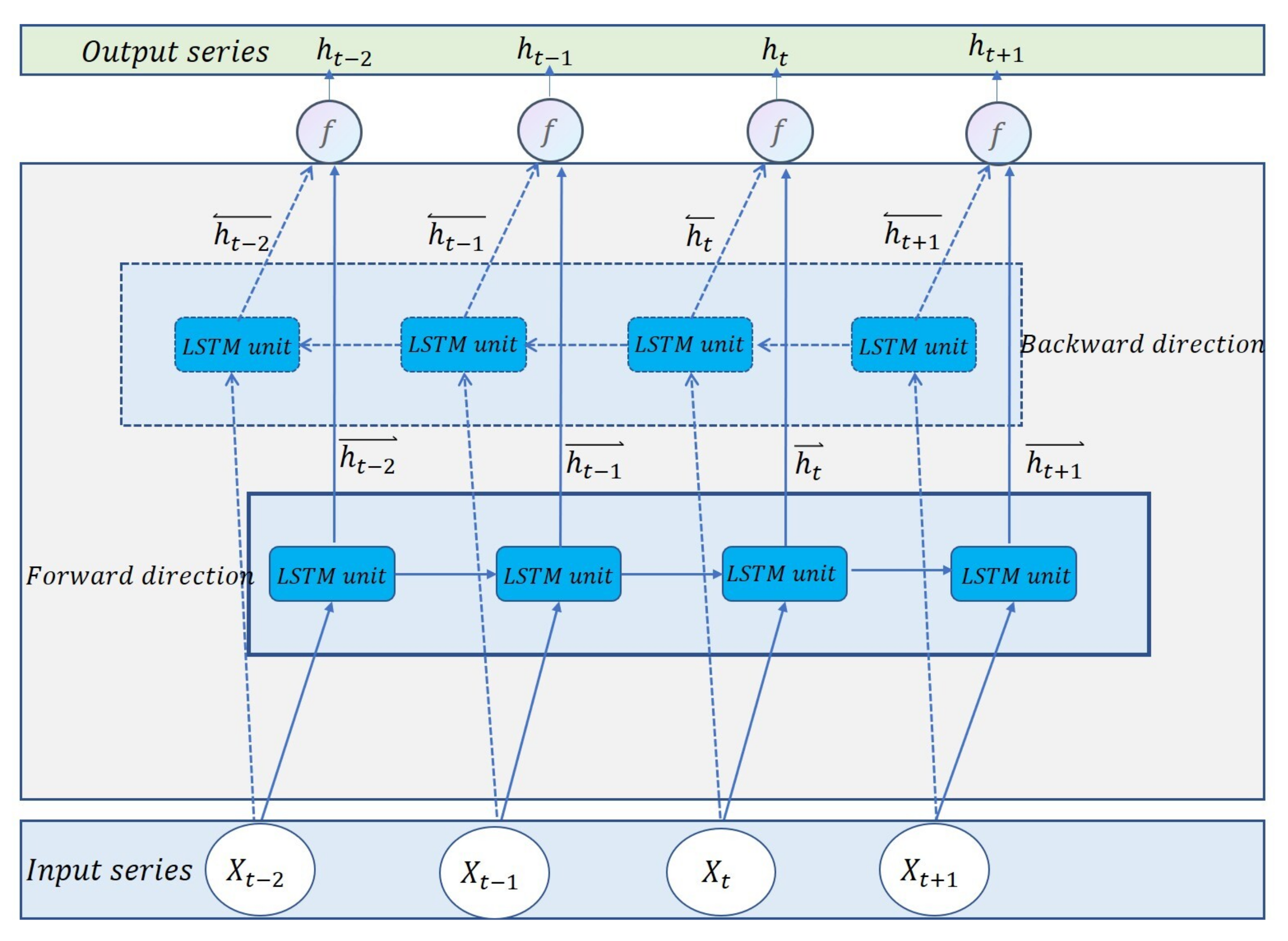
Bidirectional LSTM (BiLSTM) is a variant of LSTM which not only uses the past information, but also captures the future information. BiLSTM consists of two LSTM layers with opposite propagation directions. In the first LSTM layer, series information is delivered in chronological order, and in the second layer, series information is delivered in reverse chronological order. In each LSTM layer of BiLSTM, the computation process is consistent with common LSTM layer from Equations (1)–(6). The only difference is that the second LSTM layer of BiLSTM is reversed. As shown in Figure 2, the two LSTM layers simultaneously propagate in the opposite directions. BiLSTM combines the forward h t and backward hidden state h t sequences by a function f, which can be a summation, a concatenating, or an average function [24]. BiLSTM obtains a new sequence, and every element of it contains the previous information and future information. The process and result can be represented as:
h t = f ( h t , h t )
H = [ h 1 , h 2 , , h N ]
where h t and h t , respectively, represent the forward hidden state and backward hidden state in time step t. H represents the final series that consists of the combination of forward hidden state and backward hidden state in different time steps. N represents the length of series. In this way, BiLSTM generates a series that contains previous information and future information in each element. It easily processes a series and can capture bidirectional features of the whole series rather than directly processing a raw series. BiLSTM performs well in many time series forecasting tasks compared with LSTM models [17].
Although LSTM and BiLSTM perform well in time series forecasting, discretizing observation and emission intervals prevent LSTM and BiLSTM from acquiring deeper internal relation of time series and learn rich dynamic of series. As a continuous neural network, NODE can help to solve the above problem of LSTM while building an infinitely deep network. Both LSTM and BiLSTM structures are used in this paper to test the performance of NODE in electricity load forecasting.

3.3. NODE

Neural ordinary differential equation (NODE) is a new member of the neural networks family and is considered to be a continuous version of the ResNet [25]. Generally, the residual module of ResNet can be expressed by Equation (9):
h t + 1 = h t + f ( h t , θ t )
The residual module indicates that ResNet is discrete and undefined between different levels, and h t denotes hidden state at time t. Assuming that the network is continuous and defined between layers, naturally we will obtain:
d h ( t ) t = f ( h ( t ) , t , θ )
h ( t 1 ) = h ( t 0 ) + t 0 t 1 f ( h ( t ) , t , θ ) d t
Equation (11) indicates that by inputting any given initial value in time t 0 , we can obtain the final value after an arbitrary length of time by using a black box ODE solver such as simple Euler’s method or higher-order variants of the Runge–Kutta method [26]. Equation (10) shows that the function f defines the neural network, which is parameterized by the derivatives of h ( t ) . In this paper, we use a two-layer dense neural network to represent the derivatives of h ( t ) . Therefore, essentially, NODE can be considered as using a neural network to describe a continuous and very deep neural network.
Figure 3 shows the latent trajectory when inputting an initial value at time t 0 into NODE to propagate through Equation (11). The numbers of arrows express how many time points we set in order to observe the latent trajectory between t 0 to t 1 . In actuality, the latent trajectory means that NODE can convert any initial value into a continuous time series that exists on latent space. The ODE solver in NODE selects an appropriate step size to approximate the true solution according to the given error tolerance. Forecasting accuracy can be improved in real-time or low-power applications. Hence, NODE has two main characteristics: it produces continuous latent trajectory in time series and dynamically adapts to the real solution, which allows the NODE-based model to learn rich dynamics and continuity of time series.
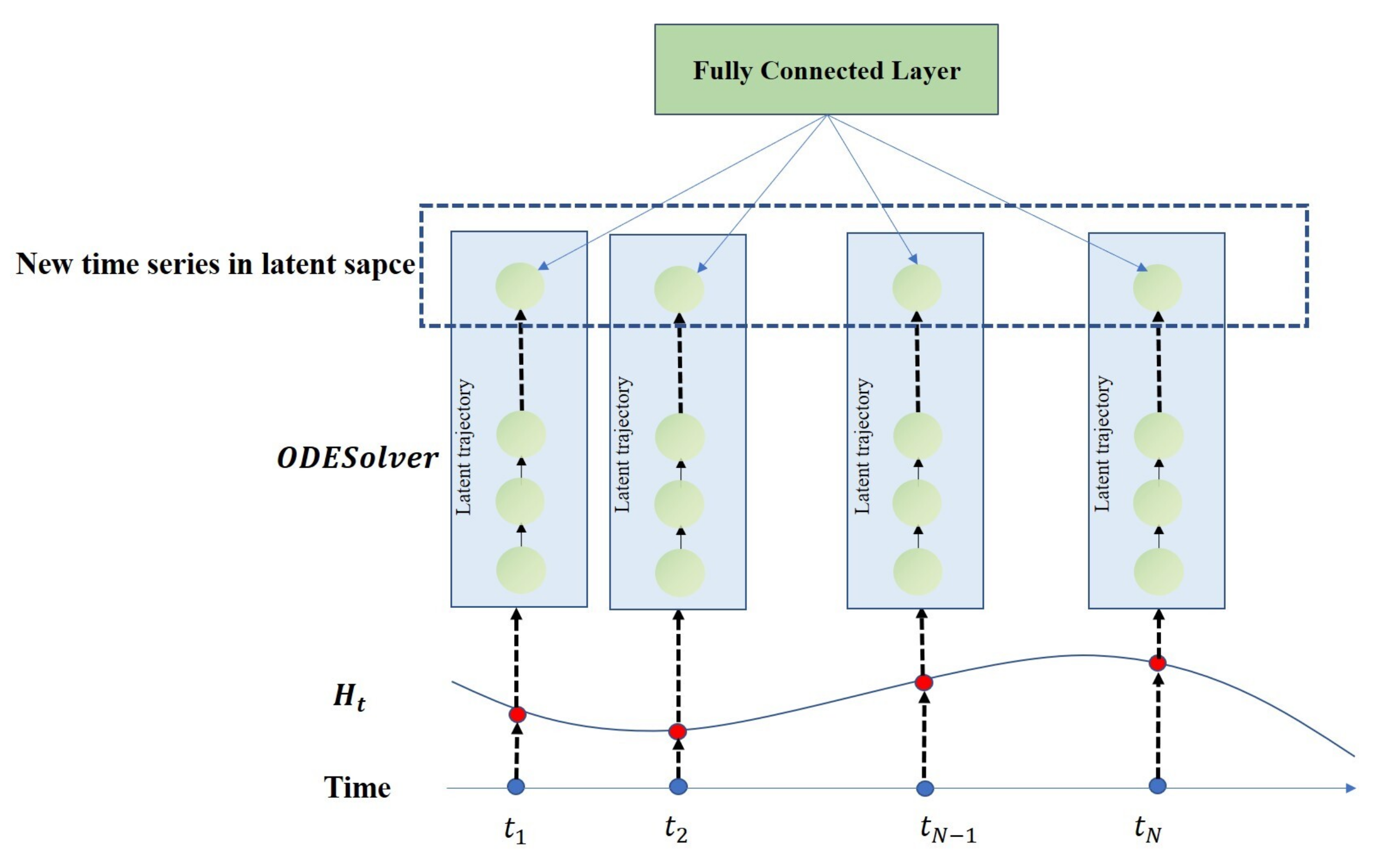
In this paper, the structure of the designed NODE block is shown in Figure 4. Firstly, we select a time series H t ranging from t 1 to t N in time. Then, each value of the time series is inputted into the same ODE solver to generate a latent trajectory in latent space, which can be considered as a time series. When each value in the original time series is input into the ODE solver, the ODE solver will produce N (N is the length of time series) latent trajectory in latent space. After that, we select the last value of each latent trajectory and combine them into a new time series in latent space. Therefore, every value in the original time series is input into the same ODE solver and generates the same number of conversions in the latent space. The information about continuous time will not be discarded. Finally, a fully connected layer is used to shorten the length of the new time series in order to refine the new time series further in latent space. In fact, NODE actually maps the original time series into a new time series in latent space, having higher continuity, dynamic, and feature information in time. It will be easier for the following LSTM or BiLSTM layer to learn the series features processes by NODE.

4. Data and Methodology

In this section, we introduce the data and preprocessing method used in this paper. We designed three types of comparative models to test the effect of NODE. Through many experiments, we choose the three models that perform the best in three metrics (root mean square error (RMSE), mean absolute error (MAE), and mean absolute percentage error (MAPE)) for electricity load forecasting. After that, we compare the models with NODE and without NODE. The detailed discussion is given later.

4.1. Data Source and Data Preprocessing

In this paper, electricity load data in Queensland Australia from 2 May to 4 July (2019–2021) were collected as our data. Data of each year are considered as an independent time series and we will evaluate our model on each time series. Data interval is half an hour, and every point in this dataset represents electricity demand at that moment.
In order to achieve a better effect, data normalization is adopted to map the data to interval between 0 and 1. It can be represented as:
X s = X X m i n X m a x X m i n
where X s is the normalized value. X m i n and X m a x represent the minimum value and maximum value of the time series, respectively.
In the experiments, we divided annual data into three parts: training set, validation set, and test set. Training set accounts for 60% of the whole dataset, validation dataset accounts for 20% of the dataset after training set, and test dataset takes the last 20% of the dataset. Models are trained on the training dataset and evaluated on the validation dataset.

4.2. Forecasting Modeling Method

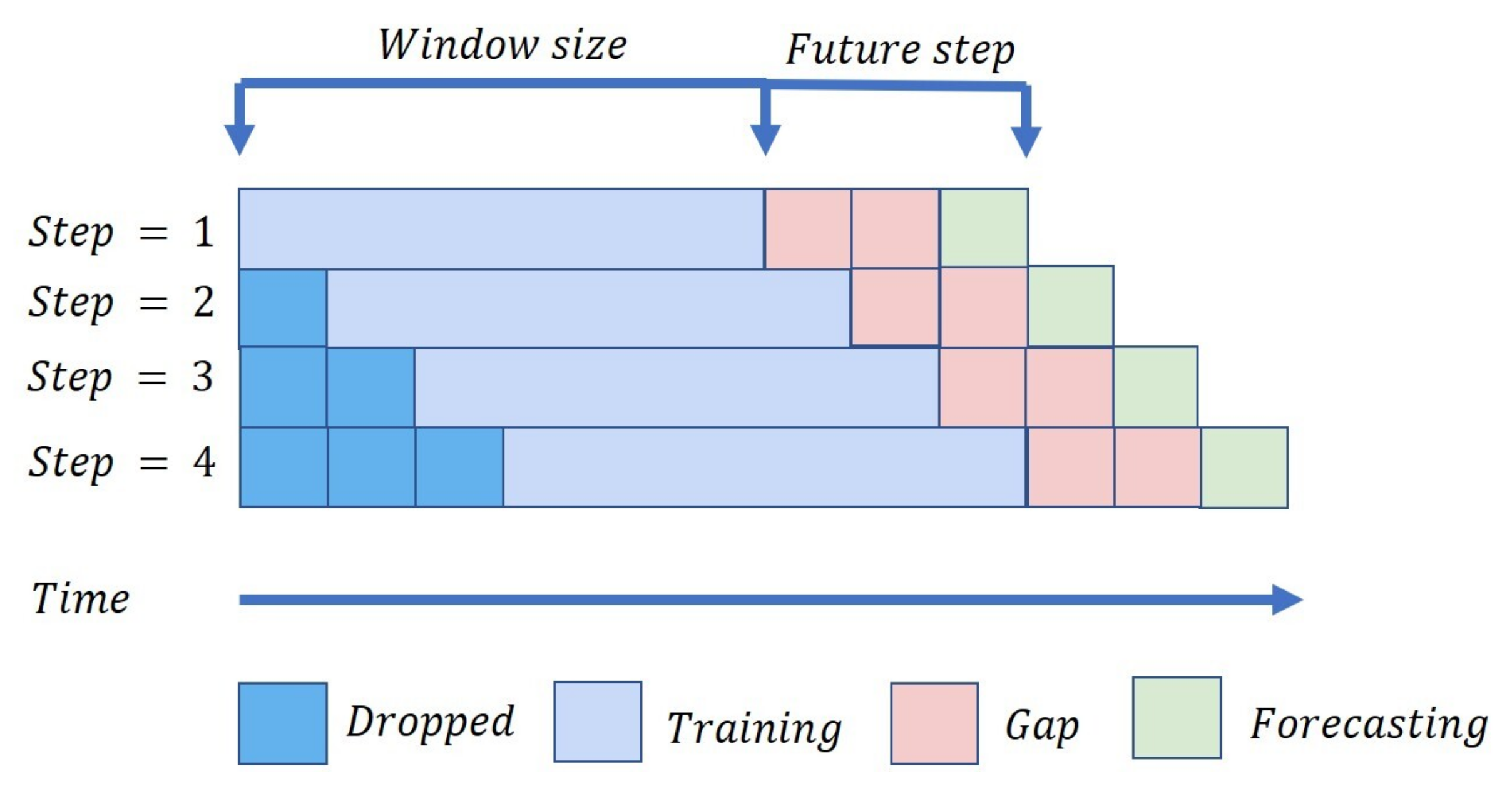
As shown in Figure 5, firstly, we need to set up the size of window and the step we want to forecast. Secondly, we slide the window forward and obtain a new window. Then, we can use the new window to make a new prediction. Every time we slide the window, we input the new window into the model to obtain a forecasting result.
In this paper, we select the window size by conducting a grid search among {10, 15, 20, 25, 30}. The 20 that achieves the best performance over the validation set is used for the test.Then, we assign time step 1, 3, 5, and 7 to evaluate the performance of our models in different forecasting steps. It means that we use previous 10 h time series data to predict electricity load in the following: 0.5 h, 1.5 h, 2.5 h, and 3.5 h. We compare the forecasting results between different steps to observe the performance of the models.

4.3. Forecasting Models

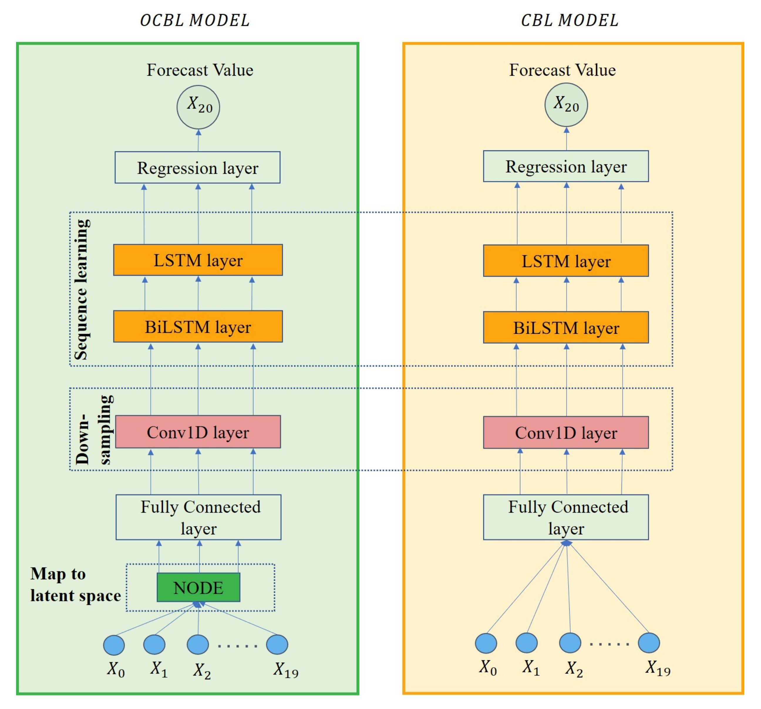
The first group of comparative models includes ODE–CNN–BiLSTM–LSTM (OCBL) and CNN–BiLSTM–LSTM (CBL). CBL mainly consists of Conv1D layer, BiLSTM layer, and LSTM layer. OCBL is based on the CBL model, and an NODE layer is added in front of the Conv1D layer. Conv1D is a convolution layer generally used in series processing, which performs well in feature extraction. The model structures of OCBL and CBL are shown in Figure 6.
The second group of comparative models is ODE–BiLSTM–stacked LSTM (OBLL) and BiLSTM–stacked LSTM (BLL). BLL combines one BiLSTM layer and two LSTM layers, and OBLL adds an NODE layer in front of the BiLSTM layer. The model structures of OBLL and BLL are shown in Figure 7.
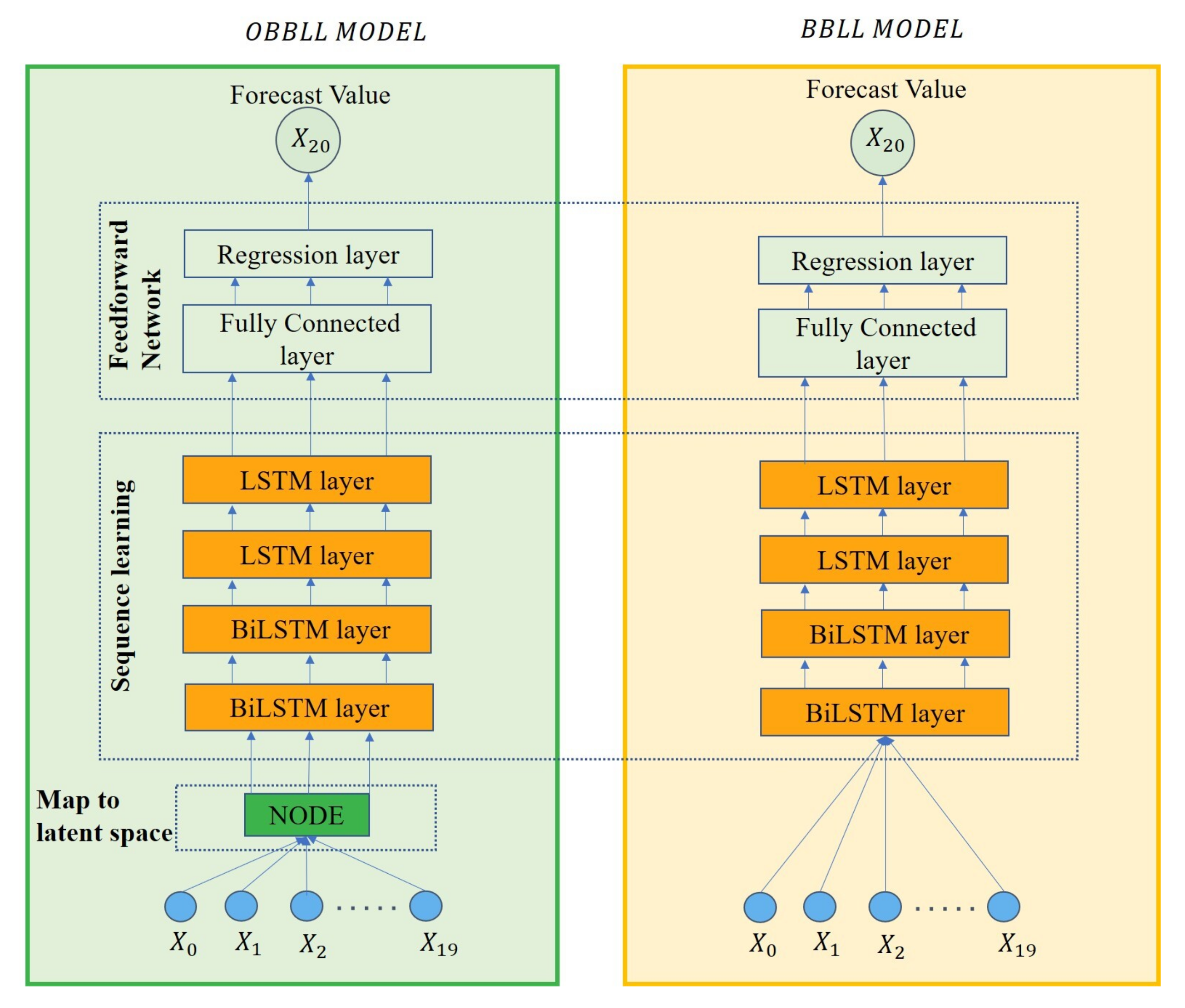
The last group of comparative models are ODE–stacked BiLSTM–stacked LSTM (OBBLL) and stacked BiLSTM–stacked LSTM (BBLL). This group is similar to the second group and the difference is that a BiLSTM layer is added in front of the original BiLSTM layer. The structures are shown in Figure 8.

4.4. Model Settings

The dataset is a univariate time series collected from 2 May to 4 July (2019–2021). One year of data has 3024 time steps, and 1814 time steps are used as training set. The size of the sliding window is set to 20. The hidden dimension of the NODE block is set as 100, which means that it has two fully connected layers with 100 hidden nodes. In order to compare the function of NODE, we use the same NODE block in different model groups. The output size of the final fully connected layer after the LSTM layer is set to 1.
The overall parameters are listed in Table 1. In OCBL and CBL, the convolutional size of the kernel is set as 3 and the number is set as 64. Then, we conducted a grid search over the size of hidden states for LSTM and BiLSTM among {20, 30, 40, 50, 60, 70, 80, 90, 100}, and the number of hidden nodes of the LSTM and BiLSTM layers achieving the best performance the over validation set is used for test (30 and 50, respectively). In the end, a fully connected layer with one node is used as the output.
In OBLL and BLL, we gradually reduce the size of hidden nodes to shorten the length of generated series to mix the rich information. In detail, we select the number of hidden nodes of the BiLSTM layer by conducting grid searches among {50, 60, 70, 80, 90, 100}. To decide the number of hidden nodes for the two LSTM layers, we conduct two grid searches over {30, 40, 50} and {10, 20, 30}, respectively. The number of hidden nodes of the BiLSTM and stacked LSTM layers achieving the best performance over the validation set is used for test (50, 30, and 10, respectively). After the LSTM layer, two fully connected layers with 50 and 20 hidden nodes are used. Similarly, a fully connected layer with single hidden node is used as model output.
In OBBLL and BBLL, similarly, we gradually reduce the size of hidden nodes. In detail, we select the number of hidden nodes of these two BiLSTM layers by conducting two grid searches among {50, 60, 70, 80, 90, 100} and {30, 40, 50}, respectively, and we select the number of hidden nodes of the first LSTM layer by conducting two grid searches among {20, 30, 40} and {10, 20, 30}, respectively. The number of hidden nodes of the stacked BiLSTM and stacked LSTM layers achieving the best performance over the validation set are used for test (50 and 30 for stacked BiLSTM; 20 and 10 for stacked LSTM, respectively). A fully connected layer with 20 hidden nodes is used and a fully connected layer with single hidden unit is used as output in the end.
In this paper, all fully connected layers use rectified linear units (RELUs) as activation function. Adam optimizer is adapted for model training. The initial learning rate is 0.001. In addition, mean squared error (MSE) is used as loss function to perform gradient descent. In order to avoid overfitting, an early stopping strategy is used to supervise the loss in the validation dataset, and the patience of early stopping technology is 10. The size of the minibatch is 32, which is selected by conducting a grid search among {16, 32, 64, 128}. Maximum epochs are set to 1000. When the loss in the validation dataset keeps not descending in more than 10 epoches, the early stopping strategy will end training. We train each model five times to obtain an average experimental result.

5. Experimental Results and Analysis

In this section, we compare the performance of three groups models, respectively, for one-step, three-step, five-step, and seven-step electricity load forecasting. Common evaluation metrics used in forecasting include SSE, MSE, RMSE, MAE, MAPE, R 2 , and so on. In this paper, we employ root mean squared error (RMSE) and mean absolute error (MAE) to evaluate our models, both of which are scale-dependent and widely used in time series prediction. In addition, we use mean absolute percentage error (MAPE) to evaluate the prediction deviation proportion in terms of the ground truth. Compared with other metrics, these three metrics reflect the accuracy of our model more intuitively and accurately. The formulas for these three metrics are Equations (13)–(15):
R M S E = 1 n i = 1 n ( y i ^ y i ) 2
M A E = 1 n i = 1 n | y i ^ y i |
M A P E = 1 n i = 1 n | y i ^ y i | y
where y i ^ represents the prediction value and y i represents the actual value of electricity load.
In the second part of this section, we compare the prediction result and actual data on testing set and observe some local differences between the prediction result and actual data.
In the third part of this section, we discuss the experimental results and explain why NODE can improve the accuracy of the combination of LSTM and BiLSTM.

5.1. Comparing Metric

In this section, we compare the prediction results of different models, and box and whisker is used to show the comparisons of different models. We only show the box and whisker in 2019 to observe the comparison of three metrics, which is similar to the comparison of the years 2020 and 2021.
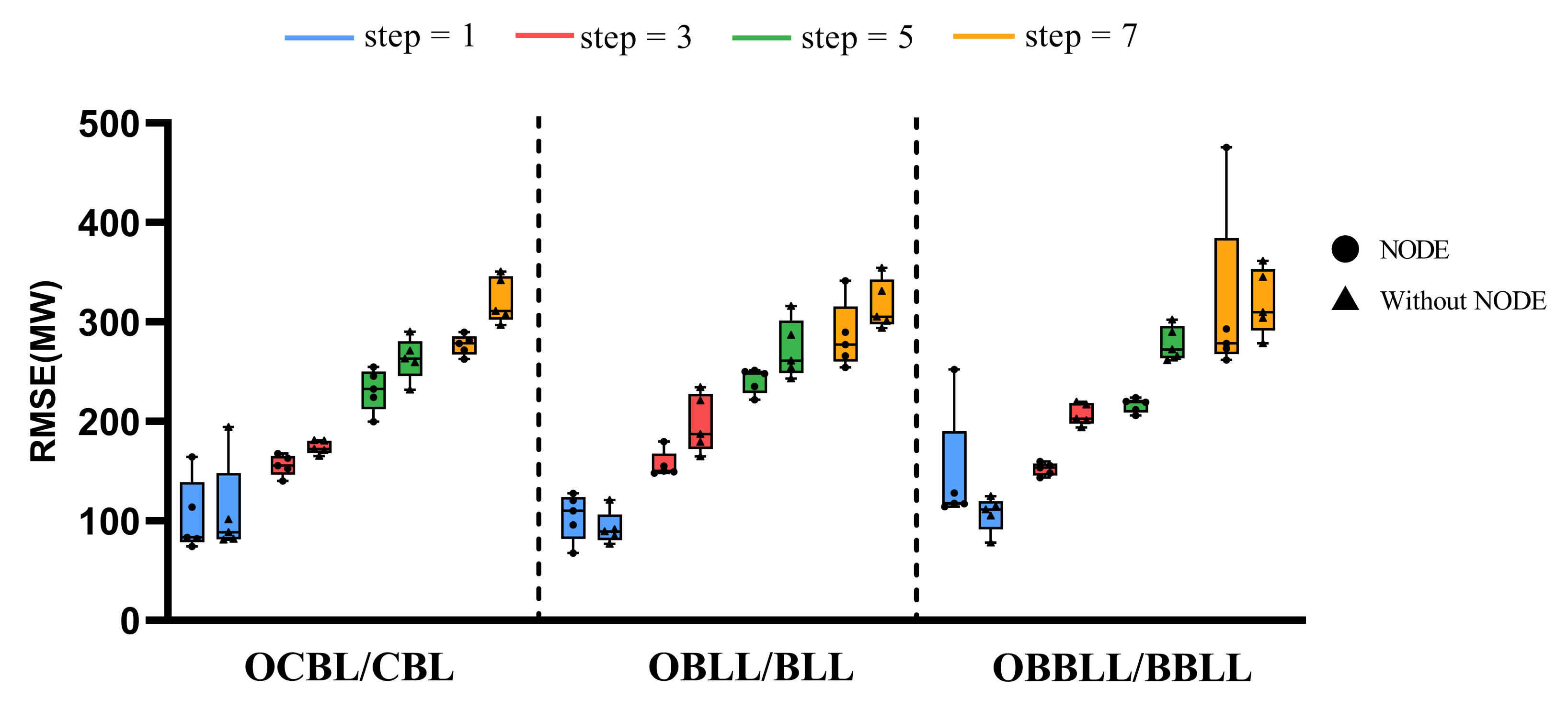
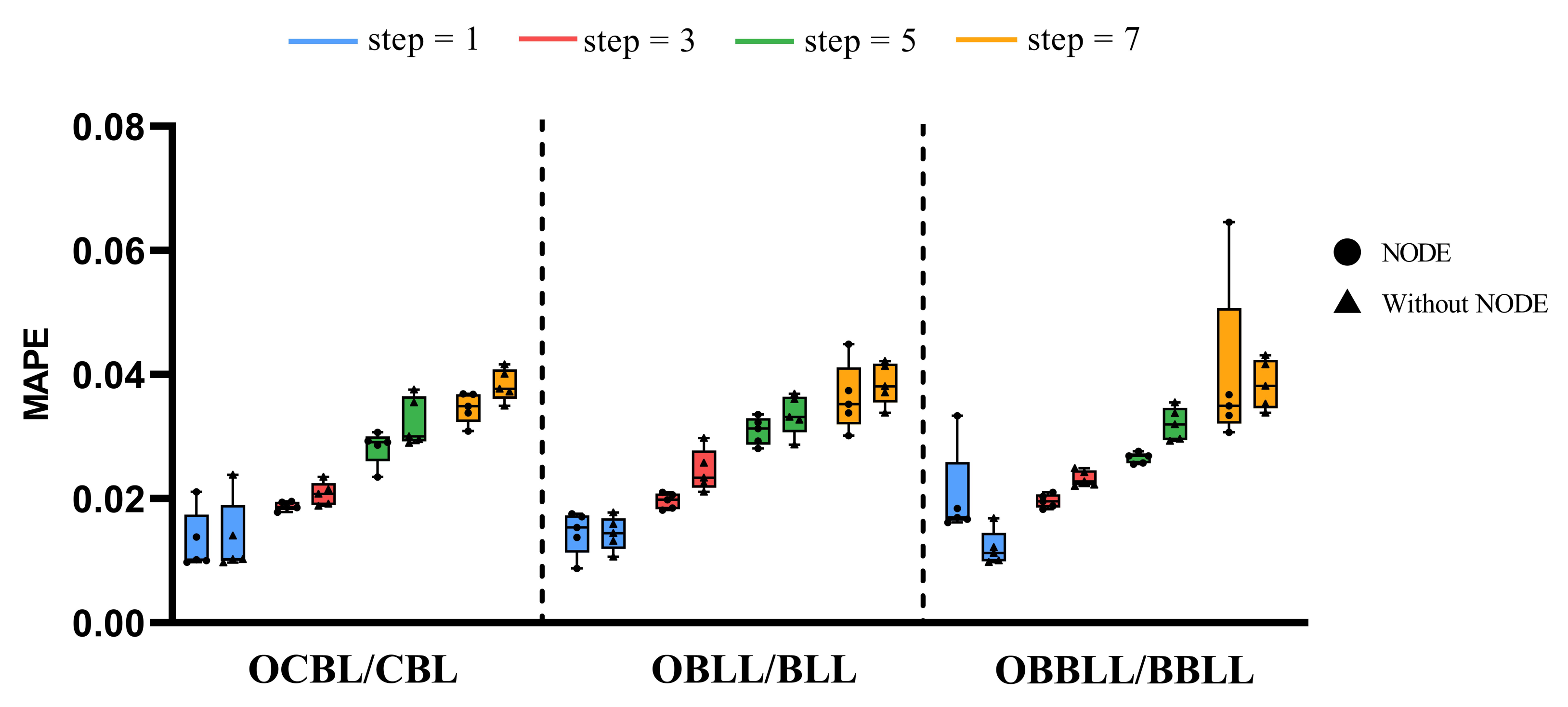
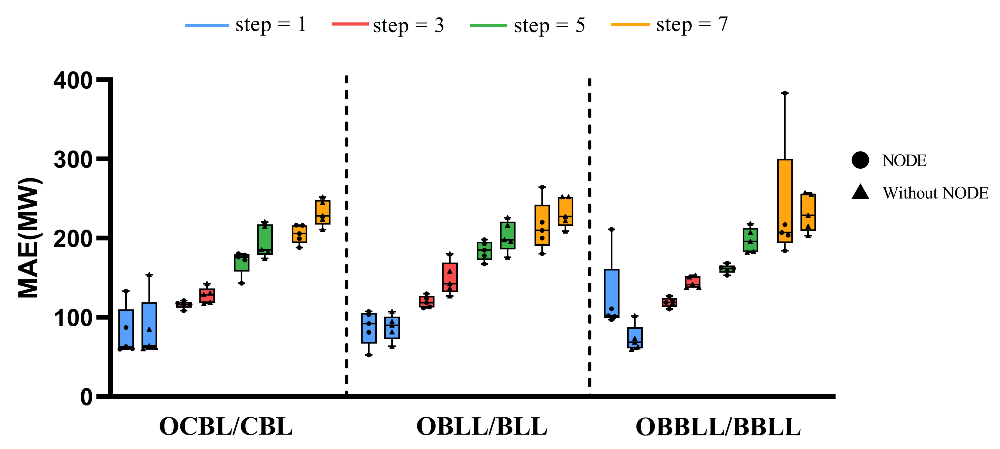
Figure 9, Figure 10 and Figure 11 use box and whisker to show the comparison of three metrics on three groups of models, respectively, for one-step, three-step, five-step, and seven-step electricity load forecasting in 2019. We can see that these three metrics rise with the increase of the future step, which means that all those models perform worse with the increase of the future step. Meanwhile, models with NODE conspicuously have advantages compared with models without NODE for three-step, five-step, and seven-step electricity load forecasting. Table 2, Table 3 and Table 4 show the comparison of 2019, 2020, and 2021. In Table 2, we can see that the average metrics of NODE models distinctly outperform models without NODE. For example, for seven-step forecasting in 2019, models with NODE outperform models without NODE in terms of RMSE, by 13.95%, 9.87%, and 1.18%, respectively. For seven-step forecasting in 2020, the improved rates of RMSE are 22.69%, 12.62%, and 12.56%. For seven-step forecasting in 2021, the RMSE reduces by 3.76%, 18.16%, and 23.58% respectively. As we can observe from Figure 9, Figure 10 and Figure 11 and Table 2, Table 3 and Table 4, generally, we can see that the LSTM and BiLSTM model with NODE is better than models without NODE. However, models with NODE seem to perform similar to models without NODE when step is 1. The reasons are discussed in Section 5.3.

5.2. Forecasting Results Comparison

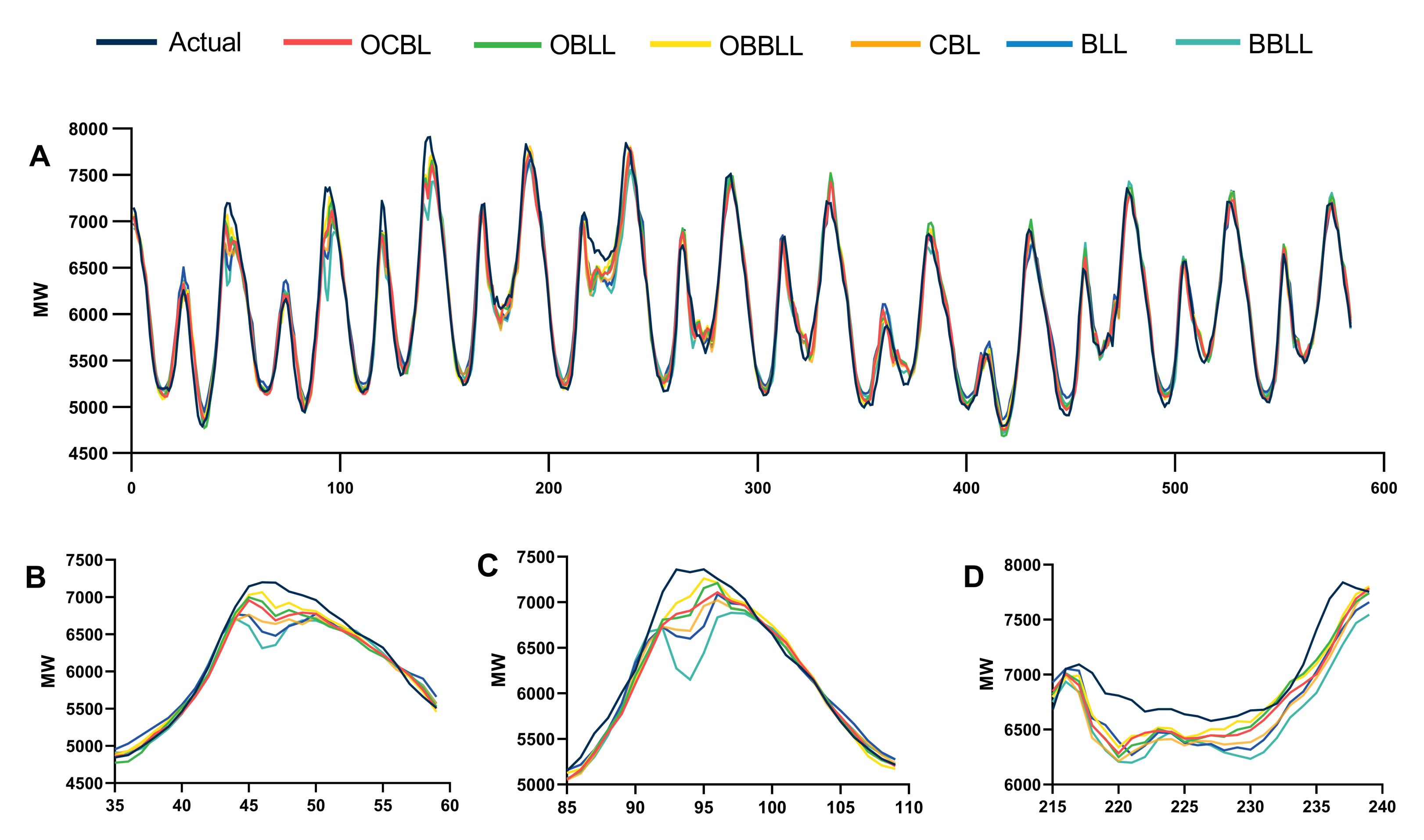
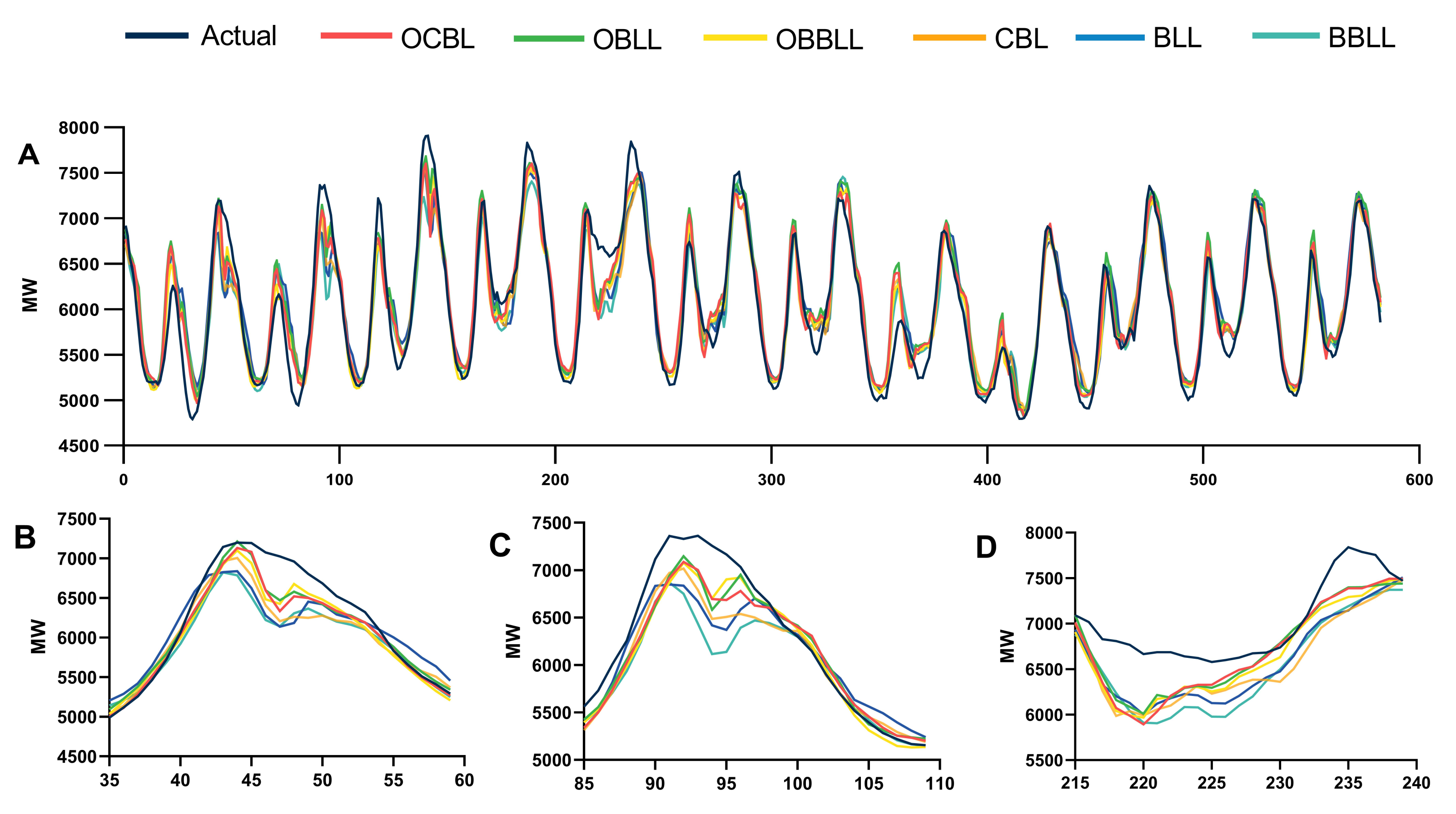
In this section, we compare the prediction results of different models. Because the trend between different steps and different years is similar, we show prediction results and their local characteristic over three, five, and seven steps in 2019.
Figure 12, Figure 13 and Figure 14 shows the prediction results and part local observation over three, five, and seven steps forecasting in 2019. As we can see from Figure 12B, there is an unpredictable peak between time step 45–50. Obviously, our model more or less predicts the peak ahead of time, while models without NODE even show a downward trend when the actual data are approaching peak. However, the prediction peak produced by NODE models uniformly closely approaches the actual peak, especially for OBBLL, compared with the prediction peak produced by models without NODE. Figure 12C also shows the same condition, but it is more intuitive and comparative because the prediction results of BBLL even have a valley in step 95 when actual data have a peak. Figure 12D is different to Figure 12B,C, and it has a normal increasing trend. We can find that all models have a forecast trends similar to actual data, but models with NODE still outperform models without NODE in prediction detail. The prediction produced by NODE models has closer curve and more similar trend with actual data in the rising process. Figure 13 and Figure 14 are similar to Figure 12 so we can obtain similar analysis results.

5.3. Experimental Results Analysis

In our paper, three groups of models were used to prove the effectiveness of NODE. Through Figure 9, Figure 10, Figure 11, Figure 12, Figure 13 and Figure 14 and Table 2, Table 3 and Table 4, we show the prediction results between NODE and without NODE. As mentioned above, although the prediction results of models with NODE for one-step seem unsatisfactory, in general, NODE can improve multistep electricity load forecasting, which means that NODE is capable of more accurate electricity load forecast when combined with LSTM and BiLSTM.
There are several reasons why NODE can improve the prediction accuracy of LSTM and BiLSTM. Firstly, as mentioned in Section 3, NODE can map the time series into latent space and shorten the series in latent space to extract features of sequence evolution relation determined by differential equation. This kind of series that is full of temporal information can make prediction remain effective even if future step becomes bigger.
Secondly, it has been reported that when modeling complex temporal behaviors, the performance of deep neural networks would significantly improve when uncertainty is inherently included in their hidden states [26]. In ODE solver, adaptive step size is adapted, which adds uncertainty to NODE and makes it more robust and flexible. This robustness can be observed in Figure 9, Figure 10 and Figure 11. Compared with models without NODE, numerical errors of NODE-based models increase slowly. This means that the NODE-based model is more robust.
Finally, ordinary LSTM and BiLSTM require discrete observation and transmission intervals, while NODE can learn differential equation relations of sequences to continuously describe the relation of features, i.e., NODE can learn the law of internal evolution equation of time series. The continuity allows the NODE-based model to learn potential dynamics to adapt acute changing of time series and capture continuous internal rules of series, which more suitably fits the trend of real-life dataset. In our model groups, stacked LSTM and its variants can capture long-term temporal dependency but they ignore nonperiodic trends hidden in discrete time intervals. In this paper, NODE is used to address this problem. As we discussed above, NODE can continuously extrapolate input series to match expected target series in latent space. In this way, nonperiodic trends hidden in discrete time intervals can be dynamically inferred by NODE. Hence, a NODE-based model has more potential to predict complex and dynamic future trends. As shown in Figure 12, Figure 13 and Figure 14, sometimes models without NODE mistakenly judge the time of peak power consumption, but NODE-based models always correctly predict the time of peak power consumption because nonperiodic trend and rich temporal dynamics are captured. In a word, with powerful continuity and dynamism, NODE captures deep nonperiodic trends and adaptively fits real-life datasets according to the input, to lower the numerical error of forecasting. Therefore, compared with directly throwing input series into a sequence learner, i.e., stacked LSTM and its variants, adding an NODE block ahead can provide continuous hidden temporal information for the sequence learner and enhance the flexibility of the model.
In addition, as mentioned above, the prediction results of models with NODE for one-step seem unsatisfactory. According to [27], focusing on recent local time series can help improve prediction accuracy. Therefore, an important reason is that when processing one-step forecasting, models tend to observe recent local time series to capture latest trends, but rich nonperiodic temporal information cannot be precisely captured because shorter local time series store less continuous information about the whole series. Therefore, the continuity of NODE is not outstanding when future step is small. In addition, adding NODE will increase the complexity and overfitting of the model when processing easy one-step forecasting. These two reasons explain why NODE-based models seem to perform similar to models without NODE when future step is one.

6. Conclusions

In this paper, NODE is applied to the STLF in order to improve the forecasting accuracy. Two-month electricity load data collected from Queensland (2019–2021) are used to validate the effectiveness of the proposed NODE. We use different types of models to verify the effectiveness of NODE. Experimental results show that NODE distinctly decreases forecasting errors on different future steps. Therefore, the combination of NODE and LSTM or BiLSTM has practical significance and can be applied in electricity load forecasting.
However, there are still some limitations of our work. The limitations of our work include the following:
  • Multivariate time series dataset is not adopted.
  • Other neural networks that can be used to parameterize the derivative of NODE are not used.
  • Long-term forecasting was not attempted.
  • Other recurrent neural networks, such as GRU and basic RNN, were not attempted.
In the future, based on remedying the above limitation, we will continue to investigate relevant aspects of NODE, including the following:
  • Investigate more forms of NODE to balance the computation memory and forecasting accuracy.
  • Apply the combination of NODE and LSTM-based models to multivariate time series forecasting.
  • Explore NODE interpolation to fill in missing values of time series.

Author Contributions

Conceptualization, S.H. and B.Y.; data curation, Q.L.; formal analysis, Q.L.; funding acquisition, Q.Z.; investigation, Q.L.; methodology, S.H. and B.Y.; project administration, Q.Z.; resources, J.S.; software, S.H.; supervision, B.Y.; validation, S.H., J.S., and B.Y.; visualization, S.H.; writing—original draft, S.H.; writing—review and editing, J.S. and B.Y. All authors have read and agreed to the published version of the manuscript.

Funding

This research received no external funding.

Data Availability Statement

Not applicable.

Acknowledgments

This work was supported by State Grid Gansu Electric Power Research Institute under Grant No. SGGSKY00WYJS2100164, No. 52272220002W.

Conflicts of Interest

The authors declare no conflict of interest.

References

  1. Hammad, M.A.; Jereb, B.; Rosi, B.; Dragan, D. Methods and Models for Electric Load Forecasting: A Comprehensive Review. Logist. Sustain. Transp. 2020, 11, 51–76. [Google Scholar] [CrossRef] [Green Version]
  2. gil Koo, B.; Kim, M.S.; Kim, K.H.; Lee, H.T.; Park, J.; Kim, C.H. Short-term electric load forecasting using data mining technique. In Proceedings of the 2013 7th International Conference on Intelligent Systems and Control (ISCO), Coimbatore, India, 4–5 January 2013; pp. 153–157. [Google Scholar]
  3. Chen, K.; Chen, K.; Wang, Q.; He, Z.; Hu, J.; He, J. Short-Term Load Forecasting With Deep Residual Networks. IEEE Trans. Smart Grid 2019, 10, 3943–3952. [Google Scholar] [CrossRef] [Green Version]
  4. Bunn, D.W.; Farmer, E.D. Comparative Models for Electrical Load Forecasting; Wiley: New York, NY, USA, 1986. [Google Scholar]
  5. Fallah, S.N.; Ganjkhani, M.; Shamshirband, S.; Chau, K.w. Computational Intelligence on Short-Term Load Forecasting: A Methodological Overview. Energies 2019, 12, 393. [Google Scholar] [CrossRef] [Green Version]
  6. Li, J.; Shui, C.; Li, R.; Zhang, L. Driving factors analysis of residential electricity expenditure using a multi-scale spatial regression analysis: A case study. Energy Rep. 2022, 8, 7127–7142. [Google Scholar] [CrossRef]
  7. Ghiasi, M.I.; Ahmadinia, E.; Lariche, M.J.; Zarrabi, H.; Simoes, R. A New Spinning Reserve Requirement Prediction with Hybrid Model. Smart Sci. 2018, 6, 212–221. [Google Scholar] [CrossRef]
  8. Ghiasi, M.I.; Jam, M.I.; Teimourian, M.; Zarrabi, H.; Yousefi, N. A new prediction model of electricity load based on hybrid forecast engine. Int. J. Ambient Energy 2019, 40, 179–186. [Google Scholar] [CrossRef]
  9. Cho, K.; van Merrienboer, B.; Çaglar, G.; Bahdanau, D.; Bougares, F.; Schwenk, H.; Bengio, Y. Learning Phrase Representations using RNN Encoder–Decoder for Statistical Machine Translation. arXiv 2014, arXiv:1406.1078. [Google Scholar]
  10. Hochreiter, S.; Schmidhuber, J. Long Short-Term Memory. Neural Comput. 1997, 9, 1735–1780. [Google Scholar] [CrossRef] [PubMed]
  11. Memarzadeh, G.; Keynia, F. Short-term electricity load and price forecasting by a new optimal LSTM-NN based prediction algorithm. Electr. Power Syst. Res. 2021, 192, 106995. [Google Scholar] [CrossRef]
  12. Chen, T.Q.; Rubanova, Y.; Bettencourt, J.; Duvenaud, D.K. Neural Ordinary Differential Equations. In Proceedings of the NeurIPS, Montreal, QC, Canada, 3–8 December 2018. [Google Scholar]
  13. Cui, Z.; Ke, R.; Pu, Z.; Wang, Y. Stacked bidirectional and unidirectional LSTM recurrent neural network for forecasting network-wide traffic state with missing values. Transp. Res. Part C Emerg. Technol. 2020, 118, 102674. [Google Scholar] [CrossRef]
  14. Nguyen, H.T.; Hansen, C.K. Short-term electricity load forecasting with Time Series Analysis. In Proceedings of the 2017 IEEE International Conference on Prognostics and Health Management (ICPHM), Dallas, TX, USA, 19–21 June 2017; pp. 214–221. [Google Scholar]
  15. Chen, Z.; Chen, Y.; Xiao, T.; Wang, H.; Hou, P. A novel short-term load forecasting framework based on time-series clustering and early classification algorithm. Energy Build. 2021, 251, 111375. [Google Scholar] [CrossRef]
  16. Li, J.; Lei, Y.; Yang, S. Mid-long term load forecasting model based on support vector machine optimized by improved sparrow search algorithm. Energy Rep. 2022, 8, 491–497. [Google Scholar] [CrossRef]
  17. Atef, S.; Eltawil, A.B. Assessment of stacked unidirectional and bidirectional long short-term memory networks for electricity load forecasting. Electr. Power Syst. Res. 2020, 187, 106489. [Google Scholar] [CrossRef]
  18. Guo, X.; Zhao, Q.; Zheng, D.; Ning, Y.; Gao, Y. A short-term load forecasting model of multi-scale CNN-LSTM hybrid neural network considering the real-time electricity price. Energy Rep. 2020, 6, 1046–1053. [Google Scholar] [CrossRef]
  19. Kuan, L.; Yan, Z.; Xin, W.; Yan, C.; Xiangkun, P.; Wenxue, S.; Zhe, J.; Yong, Z.; Nan, X.; Xin, Z. Short-term electricity load forecasting method based on multilayered self-normalizing GRU network. In Proceedings of the 2017 IEEE Conference on Energy Internet and Energy System Integration (EI2), Beijing, China, 26–28 November 2017; pp. 1–5. [Google Scholar]
  20. Han, J.; Yan, L.; Li, Z. A Task-Based Day-Ahead Load Forecasting Model for Stochastic Economic Dispatch. IEEE Trans. Power Syst. 2020, 36, 5294–5304. [Google Scholar] [CrossRef]
  21. Zhou, Q.G.; Yong, B.; Li, F.; Wu, J.; Xu, Z.; Shen, J.; Chen, H. A novel Monte Carlo-based neural network model for electricity load forecasting. Int. J. Embed. Syst. 2020, 12, 522–533. [Google Scholar]
  22. Yong, B.; Shen, Z.; Wei, Y.; Shen, J.; Zhou, Q. Short-Term Electricity Demand Forecasting Based on Multiple LSTMs. In Advances in Brain Inspired Cognitive Systems; Ren, J., Hussain, A., Zhao, H., Huang, K., Zheng, J., Cai, J., Chen, R., Xiao, Y., Eds.; Springer International Publishing: Cham, Switzerland, 2020; pp. 192–200. [Google Scholar]
  23. Han, L.; Peng, Y.; Li, Y.; Yong, B.; Zhou, Q.; Shu, L. Enhanced Deep Networks for Short-Term and Medium-Term Load Forecasting. IEEE Access 2019, 7, 4045–4055. [Google Scholar] [CrossRef]
  24. Mughees, N.; Ali, S.M.; Mughees, A.; Mughees, A. Deep sequence to sequence Bi-LSTM neural networks for day-ahead peak load forecasting. Expert Syst. Appl. 2021, 175, 114844. [Google Scholar] [CrossRef]
  25. Szegedy, C.; Ioffe, S.; Vanhoucke, V.; Alemi, A.A. Inception-v4, Inception-ResNet and the Impact of Residual Connections on Learning. In Proceedings of the AAAI, San Francisco, CA, USA, 4–9 February 2017. [Google Scholar]
  26. Xie, X.; Parlikad, A.K.; Puri, R.S. A Neural Ordinary Differential Equations Based Approach for Demand Forecasting within Power Grid Digital Twins. In Proceedings of the 2019 IEEE International Conference on Communications, Control, and Computing Technologies for Smart Grids (SmartGridComm), Beijing, China, 1–23 October 2019; pp. 1–6. [Google Scholar]
  27. Lai, G.; Chang, W.C.; Yang, Y.; Liu, H. Modeling Long- and Short-Term Temporal Patterns with Deep Neural Networks. In Proceedings of the The 41st International ACM SIGIR Conference on Research & Development in Information Retrieval, SIGIR’18, Ann Arbor, MI, USA, 8–12 July 2018; Association for Computing Machinery: New York, NY, USA, 2018; pp. 95–104. [Google Scholar] [CrossRef]
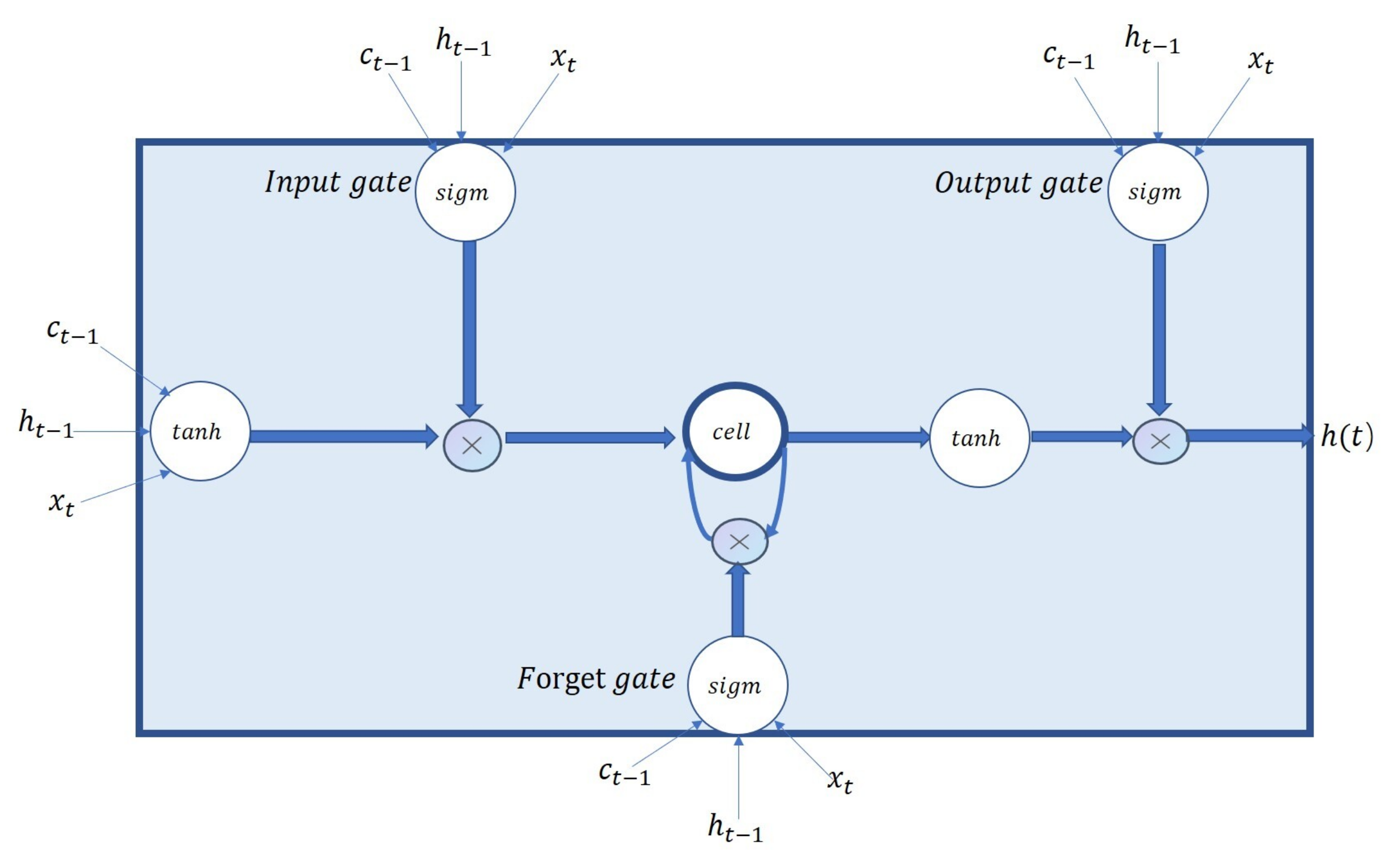
Figure 1. The structure of LSTM.
Futureinternet 15 00022 g001
Figure 2. The structure of BiLSTM.
Futureinternet 15 00022 g002
Figure 3. The latent trajectory created by forward propagation when inputting an initial value into NODE. These arrows represent the time point that is created by the adaptive mechanism of ODE solver to approach the real solution during the integration process.
Futureinternet 15 00022 g003
Figure 4. The structure of the NODE block.
Futureinternet 15 00022 g004
Figure 5. The schematic diagram of the sliding window.
Futureinternet 15 00022 g005
Figure 6. The model structures of OCBL and CBL.
Futureinternet 15 00022 g006
Figure 7. The model structures of OBLL and BLL.
Futureinternet 15 00022 g007
Figure 8. The model structures of OBBLL and BBLL.
Futureinternet 15 00022 g008
Figure 9. The RMSE metric comparison of three groups of models, respectively, in future steps 1, 3, 5, and 7 in Queensland in 2019. The dotted line divides the different comparative model groups. In each comparative model group, different colors represent different steps. The model with NODE is on the left side and the model without NODE is on the right side.
Futureinternet 15 00022 g009
Figure 10. The MAPE metric comparison of three groups of models, respectively, in future steps 1, 3, 5, and 7 in Queensland in 2019. The dotted line divides the different comparative model groups. In each comparative model group, different colors represent different steps. The model with NODE is on the left side and the model without NODE is on the right side.
Futureinternet 15 00022 g010
Figure 11. The MAE metric comparison of three groups of models, respectively, in future steps 1, 3, 5, and 7 in Queensland in 2019. The dotted line divides the different comparative model groups. In each comparative model group, different colors represent different steps. The model with NODE is on the left side and the model without NODE is on the right side.
Futureinternet 15 00022 g011
Figure 12. The prediction results and local observation for 3-step forecasting in 2019. (A) represents the whole prediction result. (BD) describe the prediction result of different local observation interval.
Futureinternet 15 00022 g012
Figure 13. The prediction results and local observation for 5-step forecasting in 2019. (A) represents the whole prediction result. (BD) describe the prediction result of different local observation interval.
Futureinternet 15 00022 g013
Figure 14. The prediction results and local observation for 7-step forecasting in 2019. (A) represents the whole prediction result. (BD) describe the prediction result of different local observation interval.
Futureinternet 15 00022 g014
Table 1. Parameter setting of the proposed models.
ModelParameterConfigurations
OCBLNumber of nodes in parameterized FC layer of NODE[100, 100]
Number of nodes in ouput FC layer of NODE[10]
Number of nodes in BiLSTM layer[50]
Number of nodes in LSTM layer[30]
Number of nodes in FC layers[100]
Kernel parameter of Conv1D layerkernel size = 3, filters number = 64
OBLLNumber of nodes in parameterized FC layer of NODE[100, 100]
Number of nodes in ouput FC layer of NODE[10]
Number of nodes in BiLSTM layer[50]
Number of nodes in LSTM layers[30, 10]
Number of nodes in FC layers[100, 50, 20]
OBBLLNumber of nodes in parameterized FC layer of NODE[100, 100]
Number of nodes in ouput FC layer of NODE[10]
Number of nodes in BiLSTM layers[50, 30]
Number of nodes in LSTM layers[20, 10]
Number of nodes in FC layers[100, 20]
Table 2. Experimental results: average RMSE, MAE, and MAPE in 2019. * indicates the model contains NODE block.
ModelRMSE (MW)MAE (MW)MAPE (%)
135713571357
*OCBL103.67155.92231.57276.9680.79115.87170.25205.221.30%1.88%2.82%3.47%
CBL109.52173.97263.20321.5484.85127.59195.62231.841.36%2.08%3.23%3.83%
*OBBL104.35156.59241.33285.8287.39119.51184.16215.021.45%1.96%3.09%3.63%
BBL106.78197.39272.31317.1387.26148.85202.27232.571.44%2.45%3.35%3.85%
*OBBLL145.98152.18216.27316.55124.51118.83161.14239.112.03%1.96%2.66%4.01%
BBLL92.73206.86278.42319.7873.03144.16197.28231.891.20%2.32%3.20%3.84%
Table 3. Experimental results: average RMSE, MAE, and MAPE in 2020. * indicates the model contains NODE block.
ModelRMSE (MW)MAE (MW)MAPE (%)
135713571357
*OCBL88.78161.19193.52235.3867.52122.31140.29172.321.12%2.05%2.31%2.92%
CBL82.01155.59231.22304.4660.31114.48172.73228.341.00%1.90%2.90%3.85%
*OBBL90.82174.30214.65275.3871.50127.59160.61203.171.18%2.10%2.71%3.50%
BBL88.56179.34259.67315.1663.66130.24192.68233.041.04%2.15%3.24%3.91%
*OBBLL103.36191.37235.04249.8282.38151.87173.95183.821.37%2.53%2.90%3.14%
BBLL87.76193.61250.28281.4064.83139.67175.77195.121.06%2.30%2.94%3.32%
Table 4. Experimental results: average RMSE, MAE and MAPE in 2021. * indicates the model contains NODE block.
ModelRMSE (MW)MAE (MW)MAPE (%)
135713571357
*OCBL115.46247.68373.69473.8795.91183.20274.13341.781.56%2.94%4.36%5.37%
CBL104.32291.99371.35492.3978.63214.72280.55362.721.24%3.36%4.50%5.75%
*OBBL142.34262.38381.87481.58112.92196.97288.11358.541.75%3.13%4.56%5.68%
BBL111.36281.34473.11588.4684.36208.37372.65453.561.33%3.27%5.94%7.11%
*OBBLL136.62244.78367.79445.90106.07181.06275.52318.911.65%2.89%4.45%5.06%
BBLL101.98281.06418.97583.4976.59210.93305.48421.331.21%3.32%4.83%6.61%
Disclaimer/Publisher’s Note: The statements, opinions and data contained in all publications are solely those of the individual author(s) and contributor(s) and not of MDPI and/or the editor(s). MDPI and/or the editor(s) disclaim responsibility for any injury to people or property resulting from any ideas, methods, instructions or products referred to in the content.