Article

Data-Driven Analysis of Outdoor-to-Indoor Propagation for 5G Mid-Band Operational Networks

1
Department of Information Engineering, Electronics, and Telecommunications, Sapienza University of Rome, 00184 Rome, Italy
2
Ericsson Research, Radio Systems and Standards, Ericsson AB, 164 40 Kista, Sweden
3
Department of Engineering Complex Software Systems, Simula Research Laboratory, 0164 Oslo, Norway
4
Department of Computer Science, Karlstad University, 651 88 Karlstad, Sweden
5
Department of Informatics, University of Oslo, 0373 Oslo, Norway
6
Rohde & Schwarz, 00156 Rome, Italy
*
Author to whom correspondence should be addressed.
Future Internet 2022, 14(8), 239; https://doi.org/10.3390/fi14080239
Submission received: 30 June 2022 / Revised: 8 August 2022 / Accepted: 8 August 2022 / Published: 11 August 2022
(This article belongs to the Special Issue Internet of Things and Cyber-Physical Systems)

Abstract

:
The successful rollout of fifth-generation (5G) networks requires a full understanding of the behavior of the propagation channel, taking into account the signal formats and the frequencies standardized by the Third Generation Partnership Project (3GPP). In the past, channel characterization for 5G has been addressed mainly based on the measurements performed on dedicated links in experimental setups. This paper presents a state-of-the-art contribution to the characterization of the outdoor-to-indoor radio channel in the 3.5 GHz band, based on experimental data for commercial, deployed 5G networks, collected during a large scale measurement campaign carried out in the city of Rome, Italy. The analysis presented in this work focuses on downlink, outdoor-to-indoor propagation for two operators adopting two different beamforming strategies, single wide-beam and multiple synchronization signal blocks (SSB) based beamforming; it is indeed the first contribution studying the impact of beamforming strategy in real 5G networks. The time and power-related channel characteristics, i.e., mean excess delay and Root Mean Square (RMS) delay spread, path loss, and K-factor are studied for the two operators in multiple measurement locations. The analysis of time and power-related parameters is supported and extended by a correlation analysis between each pair of parameters. The results show that beamforming strategy has a marked impact on propagation. A single wide-beam transmission leads, in fact, to lower RMS delay spread and lower mean excess delay compared to a multiple SSB-based transmission strategy. In addition, the single wide-beam transmission system is characterized by a smaller path loss and a higher K-factor, suggesting that the adoption of a multiple SSB-based transmission strategy may have a negative impact on downlink performance.

1. Introduction

The Third Generation Partnership Project (3GPP) recently defined the New Radio (NR) standard of Fifth Generation (5G) cellular networks [1,2], which promises to accommodate higher data rates, low latency, and massive device connectivity. The 5G NR supports a large variety of use cases and services compared to 4G Long Term Evolution Advanced (LTE-A), thanks to its numerous new features. In particular, 5G use cases include enhanced Mobile Broadband (eMBB) [3], Ultra-Reliable Low Latency Communications (URLLC) [4], and massive Machine-Type Communications (mMTC) [5]. Applications that benefit from the existence of a 5G network include autonomous vehicles, smart transportation, smart factories, agriculture, virtual and augmented reality, smart grids, and healthcare [6,7,8].
Frequency wise, 5G systems operate in the so-called low-band, high-band, and mid-band spectrum portions [9]. The low-band extends up to 2 GHz, while the high-band includes frequencies from 6 GHz and up, e.g., millimeter wave bands (mm-wave). The mid-band (refers to frequencies between 1 and 6 GHz) lies in between low and high bands; it has gained much attention lately because it offers a good balance between network capacity and coverage [9,10]. As a matter of fact, a large number of commercial 5G networks currently being deployed rely on the mid-band, and in particular on the 3.3–3.8 GHz portion, called Band n78 [11,12,13,14,15]. It is thus relevant to understand signal propagation properties in the mid-band in order to develop high-performing 5G networks.
As is well known, a signal may reach a receiver through multiple paths, due to reflection, diffraction, and scattering. Hence, a signal typically experiences both small and large scale variations in power over time. This is particularly true in indoor environments, where human activities and objects of different material, size, and geometry, affect the radio propagation significantly, eventually leading to highly dynamic propagation conditions [13,14,16,17]. Incidentally, several 5G use cases target indoor scenarios, such as smart buildings with different types of sensors, factory automation, remote control of robotic machinery, and automated vehicles in logistic applications, to mention a few [18,19,20,21]. This supports the need for an understanding of how current 5G deployments, formed by traditional outdoor base stations (BSs), provide coverage and connectivity in indoor environments.
As a result, several works dealing with the empirical characterization of the indoor channel propagation at the 5G mid-band were recently carried out [6,10,11,12,13,22,23,24,25,26,27,28,29,30,31]. In these works, the analysis was mostly based on measurements performed on dedicated, single-link testbeds, which typically did not take into account the impact of beamforming strategies, in particular single wide-beam vs. multiple SSB-based; a detailed discussion on single wide-beam and multiple SSB-based 5G strategies is given in Section 2.2.
In addition, none of the existing studies provided a systematic study of the correlation between the parameters that characterize channel propagation.
Within this context, the present paper provides the first empirical characterization of the outdoor-to-indoor propagation experienced in commercial 5G mid-band systems (in particular in Band n78) deployed in urban scenarios, based on channel measurements obtained using the Rohde&Schwarz TSMA6 Mobile Network Scanner, capable of detecting SSBs for all 5G operators within coverage and decoding the content corresponding Physical Broadcast Channel (PBCH)/Master Information Block (MIB). The study carries out an exhaustive analysis of all the relevant time- and power-related parameters characterizing channel propagation, taking into account the impact of beamforming strategies, and also includes a comprehensive correlation analysis of the parameters.
The paper is organized as follows. Related work, motivation, and contributions are analyzed and discussed in detail in Section 2. Measurement setup and data processing are described in Section 3. Section 4 provides a comprehensive analysis of time and power-related parameters that are used to characterize propagation features. The analysis includes a systematic statistical analysis aiming at highlighting the correlation between the propagation parameters. Finally, Section 5 draws conclusions and discusses future work.

2. Background, Related Work, and Contributions

This Section first provides an introduction on how channel propagation characteristics are often formalized mathematically, and on the beamforming strategies available in 5G NR. Next, it discusses relevant literature and finally highlights the contributions of the present paper.

2.1. Channel Impulse Response, Power Delay Profile, and Propagation Parameters

The Channel Impulse Response (CIR) mathematically formalizes the time and power dispersion experienced by a signal when propagating over a wireless channel. It is usually represented as the sum of all the paths a signal can undertake from a transmitter to a receiver. Paths are usually denoted as the multipath component (MPC) of the CIR, and reach the receiver at different time instants and with different power levels. The CIR of such a time-varying wireless channel, h ( t ) , can thus be written as follows [32]:
h ( t ) = n = 0 N 1 a n e j θ n δ ( t τ n ) ,
where a n , τ n , and θ n are the amplitude, delay, and phase of the nth path, and N is the total number of paths.
A well-known model for CIRs in indoor environments is the Saleh–Valenzuela (S-V) model [32]. In this model, the MPC is divided into clusters, where the power associated to each cluster and the power of the paths in each cluster decays exponentially. The interarrival times of the clusters, and of the paths within the clusters, also follow exponential distributions. Following [32], CIRs of indoor environments can be thus written as follows [32]:
h ( t ) = l = 0 L 1 n = 0 N l 1 a n l e j θ n l δ ( t T l τ n , l ) ,
where a n , l , τ n , l , and θ n l are the amplitude, delay, and phase of the nth path in the lth cluster, T l is the arrival time of the lth cluster of paths, L is the total number of clusters, and N l is the number of paths in the lth cluster.
The propagation properties of a wireless channel are usually evaluated on the so-called Power Delay Profile (PDP). The PDP is directly derived from the CIR, and shows the intensity of the received power over the different channel paths, as a function of path delays. From Equation (1), the PDP can be represented as follows:
ψ ( t ) = n = 0 N 1 a n 2 δ ( t τ n ) = n = 0 N 1 g n δ ( t τ n ) ,
where a n 2 = g n is the power associated to the nth path with delay equal to τ n .
Different propagation parameters can be evaluated on PDPs and are used to quantify time-related and power-related channel propagation characteristics.
As for time features, the mean excess delay  τ ¯ is the first moment of the PDP and measures the power-weighted average delay of all paths, that is:
τ ¯ = n = 0 N 1 g n τ n n = 0 N 1 g n .
The RMS delay spread  T τ is defined as the square root of the second central moment of the PDP, and provides a measure of the multipath richness of a communication channel. It can be calculated as follows [33]:
T τ = n = 0 N 1 g n ( τ n τ ¯ ) 2 n = 0 N 1 g n .
As for power features, the path loss quantifies signal power reduction on the transmitter-to-receiver path. It increases with the distance between transmitter and receiver and is evaluated, in dB, as follows:
P L d B = 10 log 10 P t P r ,
where P t is the transmitted signal power and P r is the sum of the power received on the N paths in the PDP, i.e., P r = n = 0 N 1 g n P t (in linear units).
The Rician K-factor is commonly used to indicate the quality of a wireless channel [34]; it is defined as the ratio between the received power of the strongest path and the sum of powers of all other paths. Mathematically, it can be expressed as follows [35]:
K R = 10 log 10 g m a x n = 0 N 1 ( g n g m a x ) ,
where g m a x is the highest gain across paths.

2.2. Beamforming Strategies in 5G New Radio

According to 3GPP Rel-15 [1], 5G NR cells may transmit up to eight SSBs. Each SSB is a composed signal that 5G cells broadcast in order to provide essential information to a 5G UE during cell searching that are needed to initiate connection procedures. In particular, an SSB consists of synchronization signals (SS), i.e., Primary (PSS) and Secondary Synchronization Signals (SSS), and PBCH, which also contains a Demodulation Reference Signal (DM-RS); hence, they are also referred to as SS/PBCH blocks. SSBs are periodically transmitted with different time/frequency patterns, depending on the adopted subcarrier spacing and frequency range. Figure 1 shows the pattern for the transmission of eight SSBs, when the subcarrier spacing adopted by the 5G system is 30 kHz. In this case, each SSB spans over four Orthogonal Frequency Division Multiplexing (OFDM) symbols in time, and the duration of an OFDM symbol is 33.33 μs.
In the frequency domain, each SSB contains 240 contiguous subcarriers within 20 resource blocks (note that the total number of resource blocks for the maximum transmission bandwidth of 100 MHz is 273) [36].
The introduction of multiple SSBs per 5G NR Physical Cell Identifier (PCI) allows for beam-based transmissions, as shown in Figure 1. In this case, SSBs with different indexes (from 0 up to 7) are transmitted over well-defined directional beams, thus allowing a 5G UE–PCI pair to identify a specific beam as their communication link, i.e., the beam corresponding to the SSB detected with highest power. Hence, when the UE is powered on, it receives SS/PBCH blocks from several PCIs, and selects the PCI/SSB pair, and thus a beam, received with the highest power. The UE will then send a preamble to this PCI/SSB in order to initiate a connection procedure that, if successful, will allow the establishment of a communication link for data exchange [37]. The detection and decoding of standardized 5G signals is of great significance in perspective of 5G NR SSB. With TSMA 6, the PBCH/MIB content of each detected SSB is decoded. The 5G NR SSB measurements help to verify 5G NR coverage and the effect of beamforming. Each SSB can be transmitted on different beam (depending on the network configuration), which can be decoded by the scanner. With different SSBs and beams, the scanner results become three dimensional: power, signal-to-noise and interference measurements for each PCI and SSB/beam index deliver a complete set of data to verify the transmission of each SSB/beam. When we have multiple SSBs/beams with their index, we can interpret the propagation characteristics of the detected SSBs/beams.

2.3. Relevant Experimental Studies

There are several works discussing outdoor-to-indoor propagation in the 5G mid-band. Among others, notable examples can be found in [24,38,39] where, however, the focus was not on the evaluation of channel propagation parameters, as it is in the present paper. In particular, the work in [24] analyzed the electromagnetic wave propagation penetration within buildings, while [38] performed measurement campaigns to investigate the channel capacity using the Weichselberger channel matrix model. Cluster characteristics of the MPC of PDPs were instead analyzed in [39], based on outdoor-to-indoor Multiple Input Multiple Output (MIMO) measurements performed in an office building.
Other works also investigated outdoor-to-indoor propagation at around 3.5 GHz, while also providing analyses of some of the channel propagation parameters defined in Section 2.1 [22,23,40,41,42]. In [22], the authors presented a path loss analysis based on channel measurements at 3.5, 4.9, and 28 GHz. Results showed that the average path loss at 3.5 GHz was lower than the one experienced at 4.9 and 28 GHz, thus highlighting that sub-6 GHz signals could penetrate concrete walls and provide nearly seamless coverage. The work in [23] studied the path loss variation due to the height difference between the transmitter and receiver via outdoor-to-indoor channel measurements at 3.5 GHz. The authors observed path loss increase with the height difference between transmitter and receiver. The work in [40] investigated the outdoor-to-indoor propagation at 3, 10, 17, and 60 GHz and observed that the RMS delay spread was weakly correlated with frequency. It was also shown that the path loss was both material- and frequency-dependent. Some statistical characteristics of channel impulse responses at 3.5 and 2.35 GHz were also studied in [41]. Results showed that the RMS delay spread at 3.5 GHz was less than the one at 2.35 GHz. The work in [42] studied the applicability of COST231, WINNER+, ITU-R, and 3GPP urban microcell outdoor-to-indoor path loss models in femtocell environments. It was shown that when the base station and the user equipment were on the same side of the street, the WINNER+ models predicted the received power with no more than 3.6 dB of R.M.S. error. Additionally, the 3GPP, COST231, and WINNER+ models predicted the received power with no more than 3.6 dB of R.M.S. error when the maximum antenna gains were used; however, smaller values of antenna gains led to estimation errors up to 14.8 dB. In [43], empirical path loss modeling was studied in an indoor to outdoor scenario for femtocells networks at 0.9, 2, 2.5, and 3.5 GHz, and a Singular Value Decomposition (SVD) technique was used to derive the path loss model parameters.
In parallel to the above works, channel characterization in the 5G mid-band was also studied in indoor-to-indoor scenarios [6,10,11,12,13,25,26,27,28,29,30,31,44]. Indeed, several empirical analyses were carried out to derive channel parameters, similarly to what the present paper aims to do for the outdoor-to-indoor case.
In [25,44], it was shown that the RMS delay spread depended on the environment size, while furniture had negligible impact. A similar analysis was carried out in [11,12] for industrial indoor environments, with main focus on RMS delay spread in both Line of Sight (LOS) and NLOS conditions. Results showed that the RMS delay spread in NLOS locations was higher than in LOS locations. References [11,26,27] focused on path loss, showing that the path loss exponent is smaller in LOS than in NLOS. Other time-related parameters were also analyzed in [26,28], showing that RMS delay spread and mean excess delay increase in presence of multiple paths.
A characterization of the S-V model at 3.5 GHz and 28 GHz was carried out in [30] in an indoor environment, and in both indoor and outdoor environments in [10]. Both studies showed that the MPC power decay factor at 3.5 GHz is lower than the one observed at 28 GHz; however, the cluster decay rate is higher at 3.5 GHz than at 28 GHz. In [13], it was also observed that CIRs at 28 GHz could be characterized by a single cluster of paths, while more than one cluster is likely to exist at 3.5 GHz. In particular, as also shown in [10], the authors highlighted that the RMS delay spread at 3.5 GHz is higher than at 28 GHz. Similarly, the path loss analysis at 3.5 GHz to 28 GHz was carried out in [11,31] an indoor environment. Both studies showed that the path loss exponent is lower at 3.5 GHz than at 28 GHz in both LOS and NLOS cases. In [6], the authors discussed RMS delay spread and path loss, showing that RMS delay spread increases with path loss. In [45], the authors presented large-scale radio channel measurements, performed in urban and suburban environments of different countries, in a frequency range from 0.8 GHz up to 73 GHz. This work presents an overview of the path loss model adopted in the recommendation recommendation ITU-R P.1411-10 (2019-08) and gives the data analysis with the approach to derive this adopted path loss model.
It is worth to highlight that this work is one of the few works that analyzes how different channel parameters (RMS delay spread and path loss in this case) are mutually correlated, thus taking a further step towards better understanding the relationships among propagation characteristics.
As anticipated in Section 1, beamforming strategy is an integral part in the design and deployment of a 5G network; however, it is worth remarking that none of the above studies addressed the impact of beamforming strategies on channel propagation characterization. A comparison table of this presented research work with the existing literature is given is Table 1.

2.4. Contributions and Innovation

The present paper provides an empirical investigation of channel characteristics for 5G systems operating in Band n78, focusing on outdoor-to-indoor propagation. The contributions of this paper can be summarized as follows:
  • An extensive set of measurements collected in an indoor environment in the city of Rome, Italy is analyzed, covering two 5G networks under deployment by two network operators. A passive channel measurement approach was used. The standardized downlink reference signals of a commercial 5G network were collected and used for extracting the channel impulse responses. The channel propagation characterization was performed based on the actual configurations applied in a commercial 5G deployed network, including the carrier frequency, bandwidth, antenna, beam-based transmission, etc.
  • Channel propagation characterization is presented for two different deployed networks, i.e., single Wide-beam and multiple SSB based 5G networks. Multipath components were extracted from measurements and used to carry out a comprehensive study of time and power-related channel parameters for different measurements locations and operators. The number of paths, interarrival times between paths, RMS delay spread, and mean excess delay are evaluated on the collected channel measurements in order to characterize time-related channel aspects. In contrast, MPC power attenuation, path loss, and Rician K-factor are studied in order to characterize power-related aspects.
  • The channel parameters’ dependencies are also studied. A comprehensive correlation analysis between the aforementioned channel parameters is carried out in order to highlight and quantify the correlation between heterogeneous propagation parameters.
Three main innovative elements can be highlighted when comparing the present work with the existing literature reviewed above: (a) Existing studies on channel characterization and analysis at 3.5 GHz were commonly based on measurements executed on dedicated, mostly single-link testbeds. In this paper, channel characterization and analysis are instead performed on measurements executed in the wild, i.e., on real 5G network deployments. This allows to derive useful insights on the indoor coverage provided by commercial 5G networks, moving towards the design and implementation of reliable and high-performing 5G systems; (b) Channel propagation characterization is presented for two different beam strategies, i.e., single Wide-beam and multiple SSB-based 5G networks. To the best of our knowledge, this is the first work presenting a comparison of channel propagation properties between a single SSB and multiple SSB-based 5G networks, since it is very hard to replicate a 3GPP standard-compliant multiple SSB-based network in a laboratory setup; (c) Existing literature did not provide a complete correlation analysis of all channel characterizing parameters. This paper instead presents a comprehensive correlation analysis by considering all channel parameters evaluated on the collected measurements.
To summarize, this is the first work characterizing outdoor-to-indoor propagation based on commercial 5G systems, providing a comparison between a single Wide-beam and multi-SSB network, using channel measurements executed in the 3.5 GHz band and with comprehensive correlation analysis of all channel parameters.
The analysis of 5G propagation channels in Band n78 provided in this work allows for a better understanding 5G propagation characteristics in indoor scenarios, and also enables further refinement of channel models towards better performance evaluation and planning of 5G mid-band networks.

3. Experimental Setup and Dataset

This section describes the measurement campaign and the adopted measurement system and setup. In particular, the collected dataset and the procedure for extracting channel measurements are presented.

3.1. Measurement System and Methodology

The data used in this work were collected as part of a large scale measurement campaigns on the cellular networks available in the city of Rome, Italy, performed between the end of 2020 and the beginning of 2021. The campaign was organized in subcampaigns, simply referred to as campaigns below, and carried out by using the Rohde & Schwarz (R&S) TSMA6 toolkit [46].
The R&S TSMA6 is an integrated system including a spectrum scanner and a laptop. In the setup adopted for the present paper, the spectrum scanner was embedded with a Radio Frequency (RF) omnidirectional antenna, and used for continuous passive monitoring of downlink control signals from operative 3GPP technologies, i.e., 5G NR, LTE, and Narrowband Internet of Things (NB-IoT). A laptop was used to run the R&S software, named ROMES, that allows for visual inspection of the ongoing campaign and for the collection of the measurements for subsequent analyses. A synchronized Global Positioning System (GPS) antenna was used for geolocating the measurements being collected. Note that other non-mobile networks cannot interfere in the 5G mid-band because the spectrum is licensed and dedicated to 5G NR; however, in case of any interference from other networks, the scanner has internal algorithms to suppress it. The TSMA6 has a time resolution of 400 n s given a good time reference (e.g., a connected Global Navigation Satellite System (GNSS) Antenna with good reception), while the estimation of the uncertainty of measurements is less than 1.5 dB. The R&S TSMA6 scanner is also significantly faster and more sensitive than a traditional spectrum analyzer in terms of the minimum quality required for the measurement; the scanner is in fact able to detect the multipath even in low SNR conditions i.e., S N R 5 dB [47]. Overall, the TSMA6 passive scanner is a system with high measurement accuracy, proposed by R&S as viable solution for accurate Electromagnetic Field measurements without the need of user calibration [48]. The R&S TSMA6 Autonomous Mobile Network Scanner with R&S ROMES4 software used in this work has been indeed adopted in 5G measurement campaigns reported in several recent scientific publications. In [49,50], the auto-calibration performed by the hardware was deemed sufficient to provide accurate channel measurements, and in [51] the power measurement accuracy of the TSMA6 was externally verified, reporting no need for additional calibration. In [52] the authors compared the data on 5G antenna placement obtained from a war-driving campaign using the TSMA6 with databases of 5G antennas available at a regulatory entity database, reporting a good accuracy of the TSMA6.
This work takes advantage of the following key TSMA6 features: (a) Automatic Channel Detection (ACD), which enables the automatic detection of operative 3GPP technologies in the spectrum bands under investigation, (b) BS positioning, which allows for estimating the position of the detected cellular BSs, and (c) MPC extraction algorithm, a built-in algorithm in TSMA6 that provides the detail of MPC for each CIR sample i.e., power associated to each MPC and its corresponding delay. Note that cellular BSs are most often referred to in terms of their PCIs or other identifiers (e.g., the identifier of the evolved Node B (eNB) for LTE), which altogether allows for their unique identification.
A set of passive measurements was collected via the spectrum scanner to be used for investigating channel propagation properties. As a matter of fact, active measurements were also collected during the campaign, by connecting a 5G commercial device (Samsung S20) to the TSMA6 and having the device run Quality of Service (QoS) and Quality of Experience (QoE) performance tests, in particular delay, throughput, and video streaming tests. Active measurements are, however, beyond the scope of this paper; further details can be found in [53].

3.2. Measurement Campaigns

Measurement campaigns were carried out in different environments, ranging from outdoor to indoor and deep indoor. Indoor measurements were collected with the receiver in a fixed position and without mobility, while outdoor measurements were collected in different scenarios, i.e., walking, driving, and riding public transportation systems. Measurement campaigns carried out without mobility included a single measurement point, geolocalized using GPS for outdoor campaigns and based on building maps for indoor campaigns. Campaigns carried out in presence of mobility included instead multiple measurement points. At each measurement point, the system simultaneously collected measurements corresponding to different frequency bands (i.e., different network operators), different technologies (i.e., 5G NR, LTE, NB-IoT), and different PCIs.
The present analysis focuses on data collected for 5G NR networks in indoor measurements with fixed receiver position and without mobility. Note that no efforts were taken to ensure static environment conditions, e.g., by preventing people from moving in the environment or performing other actions that might affect the propagation environment, such as opening/closing doors and windows. Measurements were thus collected in what are often referred to in the literature as dynamic environment conditions [54]. This choice is justified by the fact that in an outdoor-to-indoor measurement campaign using real world networks the propagation channel is in any case, for the most part, beyond the control of the experimenter. (It is worth observing however that most locations were characterized by a low variability in the indoor propagation environment, due to their positions relative to the 5G Base Station position, often including a window or a single wall obstruction. Furthermore, at the time of measurements there were very few people present in the Department, due to COVID-19-related restrictions.) It is worth observing that static conditions are typically a requirement when a threshold detector is used to identify MPCs, since multiple samples are needed in order to average out spur peaks due to noise; this approach is adopted for example in [54]; however, this is not how the TSMA6 operates: for each PDP returned by the TSMA6, each reported MPC is associated to the successful demodulation of a replica of the signal transmitted by the 5G Base Station for the PCI/SSB pair being considered and the subsequent decoding of the SIB1 information block. This means that the MPC estimation is extremely reliable, as confirmed by the R&S hardware specifications, and no averaging over multiple samples is performed.
The measurement campaigns selected for this study were performed at the Department of Information Engineering, Electronics and Telecommunications (DIET) of the Sapienza University of Rome. Table 2 provides details on the characteristics of the building and of its surroundings, as well as on the arrangement of the offices where the indoor measurements took place.
Overall, 24 unique campaigns at 8 different locations at DIET (i.e., offices and laboratories) were analyzed in this work. During these campaigns, four 5G operators were detected, including a virtual operator reusing the infrastructure provided by another operator. In order to provide statistically significant results, the analysis focused on the two operators resulting in the highest amount of data samples, called below Op1 and Op2, operating at the carrier frequencies of 3649 MHz and 3725 MHz, respectively. Finally, among all PCIs detected at each location, the analysis focused on those PCIs providing the best coverage at a given location, i.e., for each operator, those PCIs with the highest average Reference Signal Received Power (RSRP). Note that RSRP values were computed for each of the SSB that a 5G PCI transmits.
Figure 2 shows a Google Earth map of the area surrounding the DIET Department (highlighted in red). The estimated position of the two PCIs that were detected with highest average RSRP—one per operator—is also shown on Figure 2. The distance between the center of the DIET Department and Op1 PCI (resp. Op2 PCI) is of about 60 (132) meters. The specific locations at which measurements were taken are shown on Figure 3. Green, blue, and red lines represent walls, windows, and doors, respectively. Table 3 reports the summary of performed measurement campaigns for each operator and location in terms of measurement duration and total number of channel measurements considered. Measurements were performed at all eight locations; however, we did not detect any SSB from Op 1 at locations 5, 6, 7 and from Op2 at location 3. As previously mentioned, such samples refer to those PCIs with highest average RSRP across all locations under analysis, and such RSRP values refer to the SSB signals that 5G PCIs transmit, in order to synchronize with and provide information to a 5G UE.

3.3. Collected Dataset

Measurements were exported using the R&S ROMES software [55]. During the measurement campaigns, we found that both operators under analysis deployed 5G NR systems with a subcarrier spacing of 30 kHz. We also observed beam-based transmissions for Op1, with PCIs transmitting multiple SSBs (eight SSBs were detected at some measurement locations, while a lower number of SSBs were detected in other locations due to different propagation conditions), while Op2 PCIs were found to operate with a single SSB each. As an example, Figure 4 shows the received power measured at Location 1 over time for all the SSBs of the same PCI of Op1 and for the unique PCI/SSB pair of Op2 based on a single measurement campaign. The variation in the received power of different SSBs is the result of the beamforming strategy adopted by the operator, because the SSBs are transmitted at different beams. In case of operator 1, multiple SSBs are being transmitted (each SSB is transmitted via a specific beam radiated in a certain direction) with a certain interval. The received signal strength of each SSB is detected for a certain period. As all the SSB are transmitted from the same BS with a certain interval in a certain direction, therefore, all SSBs experience same power variation pattern from BS to the scanner. The variation in the power for each SSB is directly related to the environmental effects. Regarding the power variations observed between operators, these are due to the different positions of the corresponding base stations that lead to different environment effects and propagation distance. The maximum and minimum SINR for Op1 was 18 dB and 3 dB, respectively. The maximum and minimum SINR for Op2 was 24 dB and 10 dB, respectively.
As mentioned in Section 3.2, traditional MPC identification algorithms adopt a peak-detection approach that relies on a comparison with a threshold. As a consequence, a high SNR is required in order to detect peaks associated to signal replicas without mistakenly identifying spurious noise spikes as MPCs; however, as already pointed out, the TSMA6 identifies MPCs as replicas of the signal that could be demodulated and decoded. As a result, the minimum threshold for reliably detecting an MPC corresponds to the threshold for the receiver to be able to demodulate the signal, which is −5 dB according to the TSMA6 datasheet [47]. All measurements happened thus with an SINR at least 8 dB above the minimum threshold. Since there is no need to average multiple CIRs to obtain a reliable PDP, each sample collected by the TSMA6 corresponds to a PDP according to the definition provided in Equation (3) for a PCI/SSB pair detected at a given frequency carrier. The PDP is returned by the R&S TSMA6, with delay and power of each multipath component associated to that PDP. The ROMES4 software provides the details of the received peaks over the time with their corresponding powers and delay. That is, assuming that a channel composed of several paths was collected, the corresponding sample in the dataset contains: (a) the time instants at which the paths composing the PDP were received, (b) the power levels (in dBm) on each path, and (c) the total power received on the channel (note that this value maps onto the RSRP value discussed above, apart for measurement approximations).
As mentioned above, the analysis presented in this paper focuses on the channel samples for the PCIs/SSBs detected with the highest power (one per operator); however, aiming at allowing further investigation and analysis by the research community, the open-sourced dataset includes channel samples for all the PCIs/SSBs pairs detected during each campaign [56].

4. Statistical Analysis of Channel Propagation Characteristics

Based on the measured PDPs, in this section we perform an in-depth statistical analysis by investigating both time-related and power-related characteristics of channel propagation (Section 4.1 and Section 4.2, respectively). The analysis presented in the two subsections above adopts a data representation based on boxplots, generated using the MATLAB software. Boxplots are a standardized way of displaying the distribution of data based on the five-number summary (“minimum”, first quartile (q1), median, third quartile (q3), and “maximum”). The boxplot draws points as outliers if they are greater than q3 + 1.5 × (q3 – q1) or less than q1 – 1.5 × (q3 – q1), where q1 (the start of the box) and q3 (the end of the box) are the 25th and 75th percentiles of the sample data, respectively. Outliers are represented as red plus signs in the boxplots.
Following the analysis of time-related and power-related parameters, the relationship between all considered channel propagation parameters is then analyzed in Section 4.3, where a correlation analysis is reported and discussed.

4.1. Time-Related Characteristics

To measure the multipath richness of the wireless channel, the parameters of the propagation channel, such as the number of paths, interarrival times, RMS delay spread, and mean excess delay, are inspected.

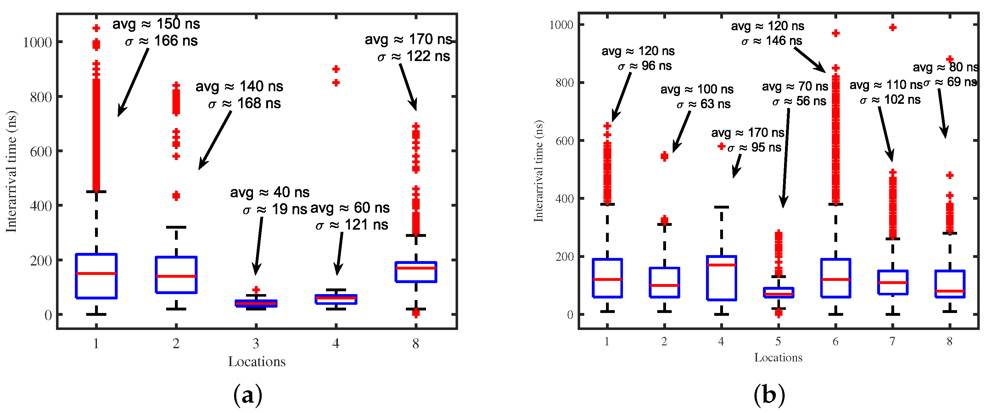
4.1.1. Number of Paths and Interarrival Times

As discussed in Section 2.1, due to multipath propagation, the signal consists of paths, each characterized by different delays and gains. Hence, the different delays of paths have an impact on the system performance and have to be considered for channel propagation characterization [57]. The boxplots with an average number of paths for Op1 and Op2 at all measurement locations are shown in Figure 5. The average number of paths for Op1 at location 1, location 2, location 3, location 4, and location 8 is 5, 5, 1, 1, and 2, respectively. For Op 2, the average number of paths at the location 1, location 2, location 4, location 5, location 6, location 7, and location 8 is 5, 6, 2, 2, 5, 5, and 6, respectively. It can be seen that the number of paths arrived at the receiver depends on the geometry of the measurement location and surroundings, rather than on the distance. Because of propagation environment variability, measurements are inherently affected by some uncertainty, which is quantified by measuring the standard deviation ( σ ) of the data. The uncertainty for each location and operator is given in Figure 5.
Interarrival time, defined as the time difference between two consecutive paths, is also a parameter of interest. Interarrival time is a random variable that depends on the wireless channel conditions. The interarrival times vary with environment, surroundings, and BS position. In the case of a sparse multipath channel, there are small delays, and fewer paths fall into a resolvable delay bin [57]; however, in rich multipath channels, the MPC may travel through different paths for a longer delay, and all paths may fall into the same delay bin [57,58]. Hence, interarrival times change with the density of MPC, which is entirely random. Figure 6 shows the boxplots with average interarrival time and uncertainty in terms of standard deviation ( σ ) , between the MPC for Op1 and Op2 at all locations. The results indicate that with a single wide beam, in the case of Op2, the interarrival times between the arriving paths are shorter than with the SSB-based transmission, in the case of Op1, when the transmission is more directive toward the measurement location.
It is worth noting that although Figure 6a apparently shows a high number of outliers for some locations, they are actually a low percentage of the total data samples. In particular, let us consider the interarrival times for Location 1 for Op1 from Figure 6a, where data samples between approximately 450 and 1000 ns are labeled as outliers. Figure 7 presents the corresponding histogram, and highlights that most of the data samples lie between 0 and 450 ns, while the data points above 450 ns that have been labeled as outliers according to the criterion previously indicated are relatively few.

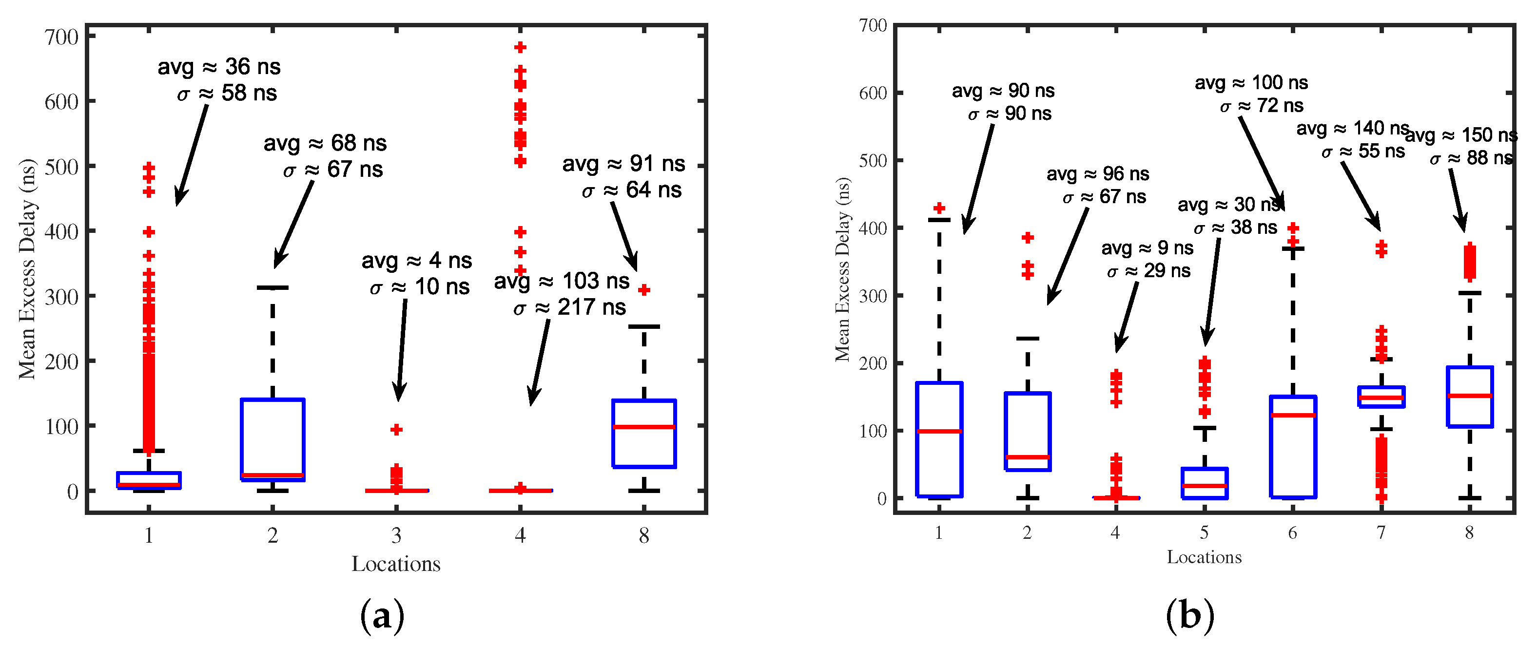
4.1.2. Mean Excess Delay

In the indoor environment, the excess delay varies with propagation distance and reflections. The length of multipath components directly depends on the environment characteristics between the transmitter and receiver. When a group of reflectors and scatterers are somewhat far away from the transmitter and receiver, the reflected multipath components experience somehow similar delays, i.e., the arrival delays will only slightly change. This is a phenomenon well known in the literature, where it is often referred to as “multipath clustering” [59]. The value of excess delay increases for the weaker reflected paths. Typically, the reflected paths from the nearby obstacles have small excess delays, while the paths reflected through remote high-rise buildings, have higher values of excess delay. The presence of a large reflector (physical objects with large size causing multipath components) causes multiple reflections, all characterized by similar delays, leading to cluster formation. The time dispersion parameter of the channel, mean excess delay, is computed for each received PDP for each operator and location. Figure 8 shows a boxplot with average of mean excess and uncertainty in terms of standard deviation ( σ ) delay for Op1 and Op2 at all measurement locations. The mean excess delay for Op1 at location 1, location 2, location 3, location 4, and location 8 is 36 ns, 68 ns, 4 ns, 103 ns, and 91 ns, respectively. For Op 2, the mean excess delay at location 1, location 2, location 4, location 5, location 6, location 7, and location 8 is 90 ns, 96 ns, 9 ns, 30 ns, 100 ns, 140 ns, and 150 ns respectively.
The mean excess delay for Op1 at locations 1 and 3, while for Op 2 at locations 2, 4, and 5, is lower than at other locations. As the excess delays vary for distance and surroundings, the signal at these locations experiences weak reflections from nearby obstacles, leading to the low value of mean excess delay. In contrast, the signal at other locations undergoes strong reflections from obstacles such as nearby high-rise buildings or human traffic, leading to larger mean excess delay. By considering the locations where the beams are more directive, i.e., location 1 for Op1 and location 6 for Op2, it can be noticed that in the 5G system operating with SSB-based transmission, for Op1, the echoes arrived at the receiver with smaller mean excess delays but were relatively weaker. While in the 5G system operating with the wide beam-based transmission, for Op2, echoes arrived at the receiver with large excess delays but were relatively much stronger.

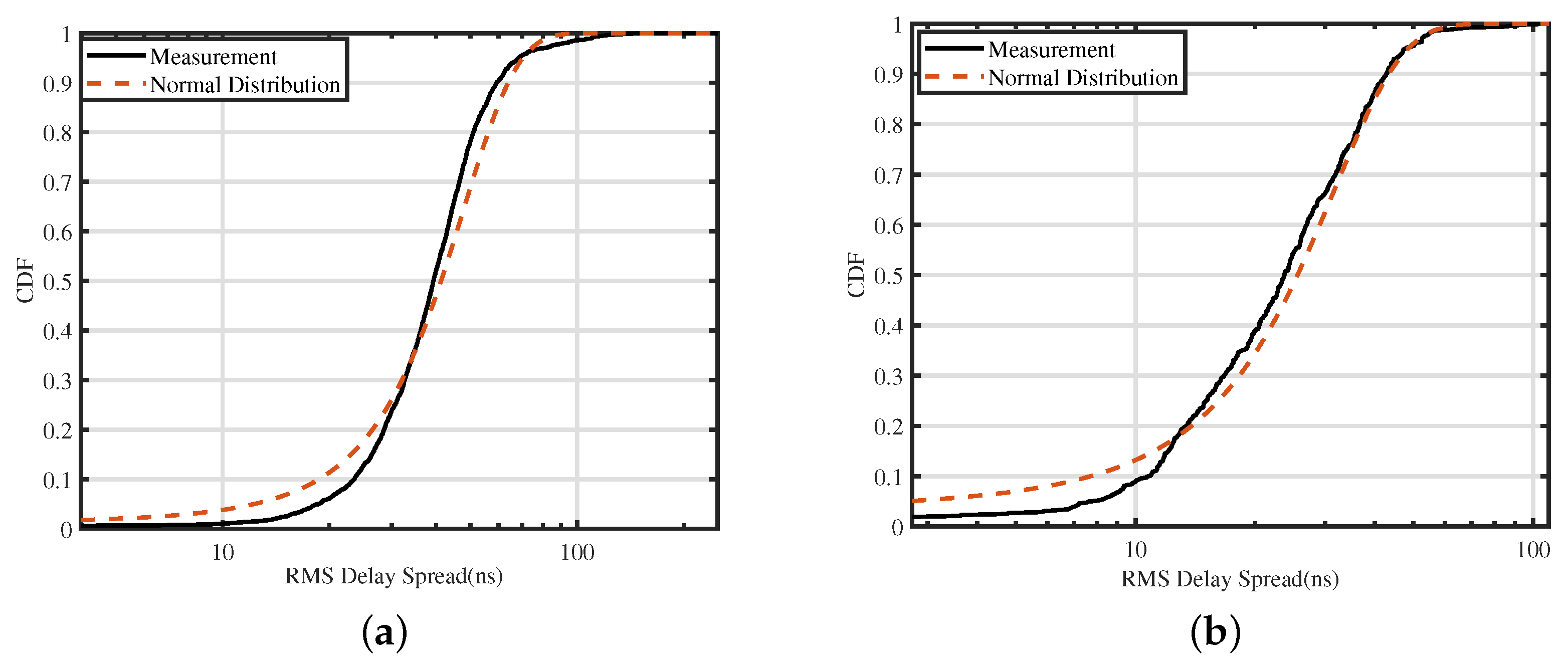
4.1.3. RMS Delay Spread

Environment has a strong effect on the delay spread. Typically, the delay spread is smaller in indoor and micro-cellular scenarios. The RMS delay spread varies with the geometric configuration and environment of the measurement location. Figure 9 shows the cumulative distribution function (CDF) of RMS delay spread of the Op1 and Op2 at measurement location 1 with best-fit normal distribution. The total number of data-points to find the curve fitting distribution for Figure 9 is 4156 (the number of data points for each location and operator can be found in Table 3). As location 1 has the highest data-points, it gives a good approximation for the CDF of RMS delay spread. Table 4 shows the mean ( μ ) and standard deviation ( σ ) of the RMS delay spread of Op1 and Op2 at all locations. The RMS delay spread for Op1 at location 1, location 2, location 3, location 4, and location 8 is 44 ns, 77 ns, 3 ns, 43 ns, and 75 ns, respectively. For Op 2, the RMS delay spread at location 1, location 2, location 4, location 5, location 6, location 7, and location 8 is 26 ns, 75 ns, 7 ns, 21 ns, 20 ns, 78 ns, and 35 ns respectively.
The RMS delay spread for Op1 at locations 1, 3, and 4 is lower than other locations. The received power is mostly due to the early received dominant path, thus resulting in a lower RMS delay spread, which explains the smaller values observed at these locations. Locations 2 and 8 have a higher RMS delay spread. Location 8 is more distant from the estimated BS position, leading to a higher delay spread with a large portion of received power through reflected paths having more significant propagation delay. In the case of location 2, while this location is spatially close to the BS, there is a wall facing the BS; as a result, signal components reach the location through reflections from nearby buildings and thus with larger propagation delays, causing a larger RMS delay spread. In the case of Op2, locations 1, 4, and 6 have a smaller delay spread. These measurement points are on the same side where the estimated BS position is, and the distance between these points and BS is smaller than other locations. Hence, at these measurement points, the signal suffers a lower attenuation. The concentration of power in the early arrived MPC is thus higher, with most of the power being received through the early received dominant path, while a smaller portion of power is received through other reflected paths; therefore, the delay time dispersion is small at locations 1, 4, and 6. Measurement point 5 also has a small delay spread, with a small propagation delay that means the strongest MPC arrived first. After that, the MPC decay quickly. We observed that measurement locations 2, 7, and 8 provided larger RMS delay spreads than other locations. All these locations are more distant from BS than the other locations. Most of the MPC arrive at the middle points of the PDP or later, and very few multipath components arrive before the middle points, which is a typical behavior for a pure NLoS propagation scenario.
The above discussion indicates that the RMS delay spread is low for the Op2 at location 6, where the wide beam is more directive. While in the case of Op1, at location 1, where the strongest SSB is more directive, the RMS delay spread is shorter than at other locations. Overall, the 5G system employing a single wide beam gives a lower RMS delay spread than the multiple SSBs-based transmission systems at locations where the beam is more directive.
Table 5 presents reported values of RMS delay spread in the literature at 3.5 GHz in outdoor-to-indoor and indoor-to-indoor environment. In [40], authors considered the outdoor-to-indoor environment and the RMS delay spread the values fluctuates from 13 to 27 ns. The values of the RMS delay spread reported in [11] vary from 20 to 70 ns in the indoor environments. It is also noteworthy to mention that the results reported in [11] establish a growing trend of the RMS delay spread with the distance, in a similar way to the results obtained in our work. As an example, for Op2, location 1, 4, and 6 is closer to the BS than compared to other locations. It is clear from the results that the RMS delay spread at locations 1, 4, and 6 is lower and higher for more distant locations. The higher delays associated with reflected and lateral waves with increasing propagation distance can explain this increase in RMS delay spread.
In [44] the value of the RMS delay spread oscillates from 5 to 22 ns in LOS and 17 to 43 ns in NLOS conditions. Another paper [12] presents the delay spread values for LOS and NLOS conditions. The authors reported values 15 ns for LOS and 24 ns for NLOS conditions, suggesting that RMS delay spread had similar values in LOS and NLOS sites. In [28], the mean value of RMS delay spread for LOS scenario is 45 ns.
It is worth noting that the results published in the literature are in line with our results; however, it should be highlighted that most of the above literature reports empirical observations for single link indoor-to-indoor deployments except one, which has single link outdoor-to-indoor deployment [40], while our results cover outdoor-to-indoor multi link real deployments, as observed in different locations; therefore, we can conclude that, from a RMS delay spread point of view, outdoor-to-indoor propagation has similar characteristics compared to indoor-to-indoor counterpart.
The best fit distribution for RMS delay spread is the normal distribution. The evaluation of the best fit distribution is based on the Akaike Information criterion (AIC). AIC is an estimator to determine the best fit distribution for a given dataset. It estimates different distribution models for the same dataset, and compares them based on the AIC scores. The distribution model with lower AIC score is better and is considered as the best fit distribution for the observed data. In our case, normal distribution is the best approximation to the RMS delay spread for both operators Op1 and Op2 at location 1 based on AIC score; however, locations 3, 4, and 8 for Op1 and location 4 for Op2 have an exponential distribution. A possible explanation for this result is the relatively small number of samples at these locations that might prevent from reliably estimating the distribution. This hypothesis is supported by the observation that in all the three locations with a high number of samples, which is location 1 for Op1 and location 1 and 6 for Op2, a normal distribution is the best approximation, as expected. The probability density function (pdf) of the RMS delay spread values in Figure 10 to show the actual data points of the RMS delay spread values.

4.2. Power-Related Characteristics
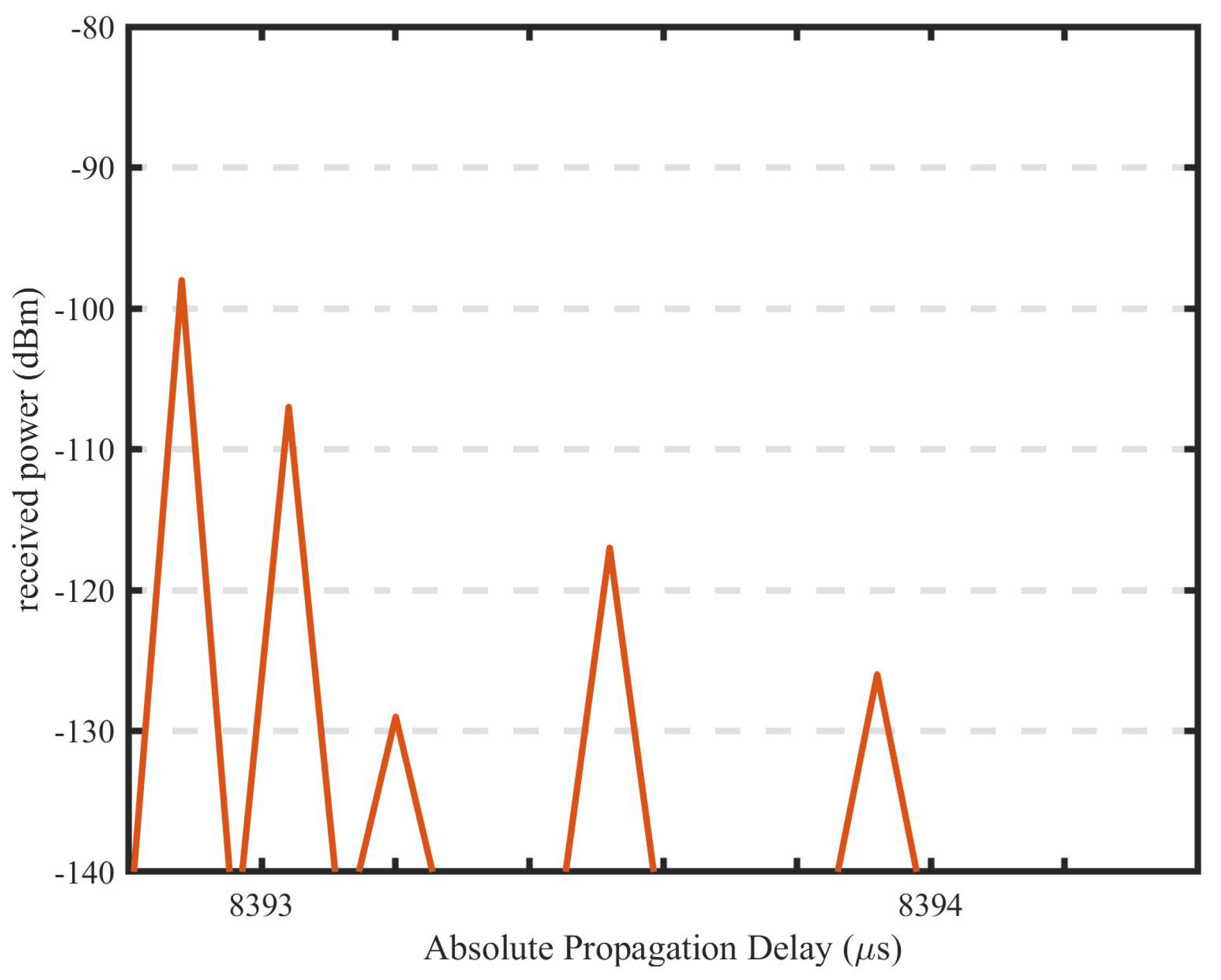
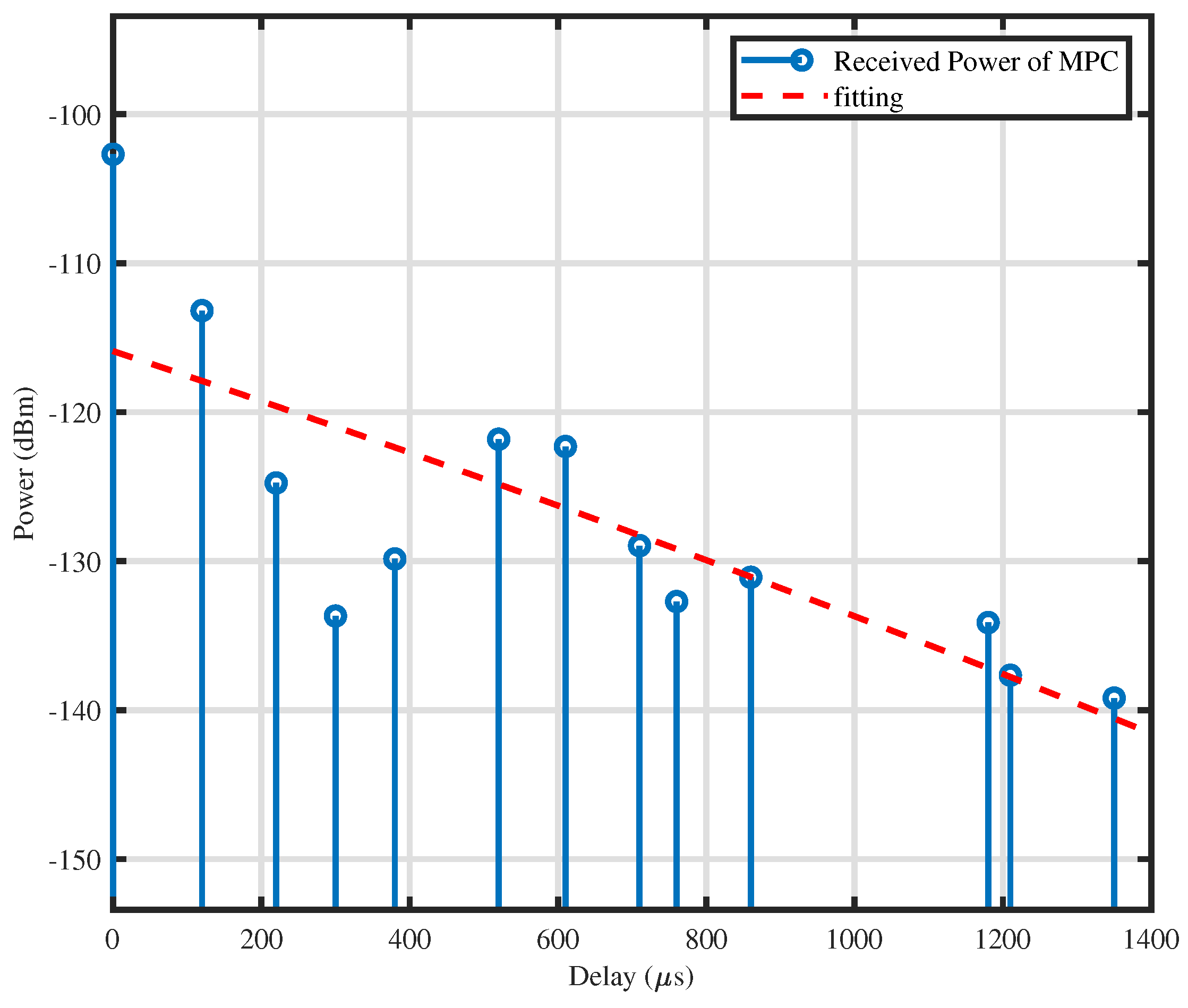
From a power perspective, the wireless channels are characterized by the fluctuations in the received power, i.e., the signal’s strength at the receiver. The received power decreases as the signal travels for a longer distance, typically as a result of reflected paths vs. the direct path. An example of single measured PDP is shown in Figure 11. Based on the measurements, the noise floor for the TSMA6 was estimated to be about −123 dBm for 5G NR. As already mentioned, the TSMA6 is able to operate with low SNR values (−5 dB) because it performs coherent demodulation of the System Information Block (SIB) signal for each path. In this section, we discuss the power-related characteristics of the wireless channel, such as pathloss, K-factor, and power decay.

4.2.1. Power Decay

According to S-V channel model, the amplitudes of the MPC decay exponentially due to the multiple reflections in the vicinity of the transmitter and receiver [59]. The propagation delay and the power attenuation (in dBm) of the reflections increase roughly linearly with the number of reflections, leading to an exponential decrease in the amplitude of reflections as delay increases [59]. Our purpose is to investigate and show the power decay behavior in case of real deployed network measurements. An exponential decrease was indeed observed in our data, as seen in Figure 12, showing a typical PDP measured at Location 1 and the corresponding exponential fitting, represented as a red dashed line. For the given PDP, the MPC decay follows an exponential relationship with delays, which translates into a linear decay when the received power is in the dB scale. This result is in agreement with the results discussed in the literature [60,61,62,63]. For the fitting, we used MATLAB curve fitting toolbox [64]. This toolbox offers the linear fit with goodness-of-fit (GOF) of 62% for the measured PDP in Figure 12. Similar fittings can be obtained for other measurement locations and both operators.

4.2.2. Pathloss

The Pathloss (PL) is calculated based on the downlink reference signal. This downlink reference signal is determined by the SS/PBCH block index and the estimated PL based on the SS/PBCH block index is given as:
P L = R e f e r e n c e   S i g n a l   P o w e r     R S R P
where the reference signal power is the average energy per resource element and is determined by the parameter SS-PBCH-Block Power. In our measurements, the reference signal power for Op1 and Op2 is 14 dBm and 11 dBm, respectively. The boxplots and average value of the PL for Op1 and Op2 at all detected locations are shown in Figure 13. Path loss is influenced by many factors such as the distance between the transmitter and the receiver, antenna height, environment, reflections, scattering, absorption, etc. From the boxplots, we can observe the relationship between the PL and the distance. In general, PL increases with the distance, and this can bee seen from the the OP1 case, where the locations are roughly ordered in increasing distance from the BS. It shows that as the distance between the BS and the measurement location increases, the path loss also increases. With an increase in distance, the signal undergoes more attenuation that increases the PL. We can also see a similar trend in the case of Op2, where locations 1, 4, and 6 are closer to BS than the other locations; therefore, the signal experience less attenuation at these locations; this leads to a decrease in PL.
The measured PL at different locations of DIET department are also compared with predictions from the model 3GPP (UMi). The Friis Free Space Path Loss (FSPL) is also shown as a reference. The FSPL and PL using 3GPP (UMI) model is calculated by taking the estimated distance between the base station and the measurement locations. For Op1, the measured PL is on average about 20 dB higher than the PL predicted by the 3GPP model. The reason for this difference is an effect of being an indoor measurement, directivity of SSBs, distance errors, etc. In case of Op2, the PL estimation by 3GPP model is more accurate. A possible explanation for this difference is that the 3GPP model does not account for SSB-based transmission, leading to a PL estimate for single wide-beam-based transmission (for Op2) more accurate than for the SSB-based transmission (for Op1).

4.2.3. Rician K-Factor

This section illustrates the results for the K-factor for both operators and all locations. The CDF of the measured K-factor for the strongest PCI for the Op1 and Op2 at the measurement location 1 is shown in Figure 14. The measured K-factor for each operator and measurement location fits very well to the normal distribution. Based on the AIC estimator, normal distribution is the best approximation for the K-factor values for both operators Op1 and Op2 at location 1. Similar distribution fittings can be obtained for other measurement locations. The mean and standard deviation values for the K-factor are given in Table 6. The mean value of the K-factor for Op1 at locations 1 and 2, and Op 2 at locations 1, 4, and 6, is higher than other locations. At these locations, the K-factor value is far greater than 0 dB. In the case of Op1, locations 1 and 2 are closer to BS and less obstructed than other measurement points; as a result a significant part of the received power is associated to the dominant path, with a small number of paths. Similarly, locations 1, 4, and 6 have higher K-factor values, so it is more likely that there would be few paths, including a strong path that leads to a higher K-factor value. The main reason for high k-factor values at locations 4 and 6 is that the BS and locations 4 and 6 face directly without any obstruction by walls. The only obstruction was the glass window, opened at the time of measurement; hence the channel at locations 4 and 6, for Op2, is more LOS-alike; therefore, K-factor increases when the channel is more LOS-alike with a small number of weak reflected and scattered NLOS paths.
At other measurement points, the signal is greatly obstructed and major portion of the power is received through NLOS components, with a very small direct path power. We also postulate here that the beam is not highly directive towards these locations, and a portion of power is received through the reflections due to the objects and nearby buildings.
It can be observed that the K-factor varies with the location. The K-factor is particularly high when the beam is more directive toward the measurement location, and the distance between the base station and the measurement’s location is small. Overall, the 5G system employing a single wide beam gives a higher K-factor at locations where the beam is more directive than the multiple SSBs-based transmission systems. Figure 15 shows the actual data points of the K-factor values and the presence of two peaks in the probability density function (pdf) of the K-factor due to channel variations.

4.3. Correlation Analysis

Statistical channel models are attractive for their simplicity but they sometimes lack accuracy. In order to improve the statistical channel modeling, it is of key interest to derive information on the time/power variability of the propagation parameters. Interdependence of radio-channel model parameters, being observed in some measurement data, should also be reproduced by the channel model. To this purpose, the statistical correlation between the channel propagation parameters from measured data helps to obtain reliable models that reflect the true propagation environment. Based on the existing literature, one can expect the time dispersion parameters, i.e., mean excess delay and RMS delay spread, to be positively correlated with PL [6], while the K-factor is typically negatively correlated with time dispersion parameters [65,66]. In this work, we are considering all the channel propagation parameters for correlation analysis to give a clear idea of which parameters are correlated and which are not. This analysis will allow us to answer the following questions:
Do the estimated channel parameters, i.e., the number of the paths, interarrival times, mean excess delay, RMS delay spread, PL, and k-factor, interact with one another? Are they correlated? If yes, could we predict that they were? Our prediction is if the number of paths increases, there will be an increment in mean excess delay, RMS delay spread, and PL, and decrement in the interarrival times and k-factor. If the value of interarrival times decreases, the time dispersion and PL will increase, and the k-factor will decrease. In addition, if the time dispersion increases, PL will increase, and the k-factor will decrease.
We performed a correlation analysis between all the estimated channel parameters based on the collected dataset. We performed Spearman rank correlation test to measure the degree of association between the parameters. The Spearman correlation indicates whether a monotonic relationship exists between the two variables, and can be considered as a more general indicator compared to the Pearson correlation, which indicates whether a linear relationship exists. We also performed Pearson correlation and, as expected, the values of Pearson correlation coefficient are lower than the Spearman correlation coefficient values.
Correlation tests were performed in MATLAB and then confirmed using the SPSS software [67]. Results indicate that the correlation of the parameters is independent of the measurement locations and operators. By changing the measurement location and operators, the correlation coefficient values may change; however, the statistical association of the parameters remains the same; therefore, we are giving a correlation analysis of both operators and all locations collectively. The correlation coefficients of all combinations of the estimated channel parameters are shown in Table 7. To give a more clear idea about the association of the channel parameters with each other, we considered a threshold ± 0.2 for correlation coefficient. It means if the correlation coefficient for any pair of parameters is between −0.2 and +0.2, then there is no correlation.

Discussion

From the table, we can see that the number of paths positively correlates with both time dispersion parameters, i.e., mean excess delay and RMS delay spread, and PL. The increase in mean excess delay with the number of paths is caused by the higher delays associated with reflected and lateral paths, since the LOS path is obstructed by doors and walls, leading to several reflections. This shows that as the channel becomes richer in multipath, the excess delay, which is a delay of any path relative to the first arriving path, increases as the power of arriving paths decreases. In the outdoor to indoor channel, the remote high-rise buildings produce strong reflections with large excess delay. Similarly, the RMS delay spread is the power-weighted standard deviation of the delay of reflected paths; therefore, an increase in RMS delay spread with the number of paths is caused by the increased spread of delays of paths. The RMS delay spread and mean excess delay depend on the delay of the multipath components. As the delay of the multipath components increases, there will be an increased excess delay and delay spread. As expected, there is a positive correlation between RMS delay spread and mean excess delay.
Similar to excess delay and RMS delay spread, PL also positively correlates with the number of paths. With an increase in distance between BS and measurement location, it is more likely that the reflected paths carrying a significant amount of power will be obstructed by the obstacles such as rough walls, trees, etc., which absorb and scatter them. As a result, the received signal contains scattered paths; therefore, the number of paths that carry a significant amount of power decreases with an increase in distance that also causes an increase in PL.
When the mean excess delay and RMS delay spread increases caused by the higher delays associated with reflected and lateral paths, the power corresponding to these paths decreases, leading to increased PL. Further, these delays increase with increasing distance due to scattering. It shows a linear dependency of PL on the time dispersion parameters, and our results show, as expected, a positive correlation between time dispersion parameters and PL.
There is a negative correlation between the number of paths and the K-factor because the dominant path becomes weaker due to scattering. The decrease in the power of the dominant path leads to a decrease in the K-factor value. As the RMS delay spread and mean excess delay increase due to the increased number of paths with larger delays and their corresponding reduced power, K-factor decreases. Further, PL increases with decreasing power, and the K-factor decreases, which explains the negative correlation between K-factor and PL and time dispersion parameters.
Our analysis shows a weak negative correlation between interarrival times and other channel parameters. This is due to the fact that the interarrival times are closely linked to the measurement location’s environment, surroundings, and BS position. They may vary for each CIR due to the time-varying nature of the wireless channel. In the case of a sparse multipath channel, there are small delays, and fewer paths fall into a resolvable delay bin; however, in rich multipath channels, the MPC may travel through different paths for a longer delay, and all paths may fall into the same delay bin. Hence, interarrival times changes with the density of MPC, which is random; therefore, there is no well-defined correlation between the interarrival times and other channel parameters.
Conclusively, both time dispersion parameters are positively correlated with each other and also with the number of paths. PL has a positive correlation with time dispersion parameters and the number of paths. The K-factor is always negatively correlated with time dispersion parameters, PL, and the number of paths. In contrast, interarrival times do not show a well-defined correlation with any other channel parameter due to their random behavior with channel conditions.

4.4. Discussion

Based on the above analysis, the following observations could be highlighted:
  • The 5G system operating with SSB-based transmission, the echoes arrived at the receiver with smaller mean excess delays but were relatively weaker. While in the 5G system operating with the wide beam-based transmission, echoes arrived at the receiver with large excess delays but were relatively much stronger.
  • The RMS delay spread is lower for the 5G system, using a single wide beam, than the multiple SSBs-based transmission systems.
  • The system with multiple SSB-based transmission, the measured PL is on average about 20 dB higher than the PL predicted by the 3GPP model. While in case of single wide-beam-based transmission, the PL estimation by 3GPP model is more accurate. A possible explanation for this difference is that the 3GPP model does not account for SSB-based transmission, leading to a PL estimate for single wide-beam-based transmission more accurate than for the SSB-based transmission.
  • The 5G system employing a single wide beam gives a higher K-factor than the multiple SSBs-based transmission systems.

5. Conclusions

In this paper, the radio channel characteristics of the 3.5 GHz 5G-NR band were analyzed based on the results of a measurement campaign on deployed commercial 5G networks, performed in a typical urban scenario with the receiver set at multiple indoor locations. A preliminary analysis of the results identified the presence of two operators working with different beamforming strategies, adopting a single wide-beam SSB vs. multiple SSBs.
In general, the analysis of both time and power-related channel parameters confirmed the behavior observed for 5G signals in previous investigations: the reception of the signal in an urban environment is highly dependent on the building density and the traffic, leading to large variations in the time-related parameters as well as path loss and K-factor values. An exhaustive correlation analysis also confirmed partial results presented in past investigations: a positive correlation between the time-related parameters and PL and the number of paths was observed. The K-factor negatively correlated with time dispersion parameters, PL, and the number of paths.
The analysis highlighted however marked differences between the two beamforming strategies. The 5G system adopting multiple SSB-based transmissions showed higher RMS delay spread and mean excess delay values as compared to the system employing single wide beam. Furthermore, single wide-beam based transmission experienced a smaller PL than SSB-based transmissions, and the average PL estimate by 3GPP model is more accurate for wide-beam-based transmission than for SSB beam based transmission. In addition, single wide-beam transmission leads to a higher K-factor and smaller inter-arrival times as compared to multiple SSB-based transmission, although the two beamforming strategies show a similar average number of multipath components arriving at the receiver.
In conclusion, a single wide-beam beamforming strategy is characterized by better propagation conditions, and promises thus better network performance. While further investigations are required to confirm this trend in different locations and propagation environments, this result is a first indication on the impact that beamforming can have on the performance of a 5G network, and can provide valuable insight in the design of new 5G networks and in the extension of existing ones. This is particularly relevant in light of the expected deployment of standalone 5G NR networks that will allow for a network design specific for 5G NR propagation characteristics.
Future work will focus on the tuning of a channel model at 3.5 GHz for outdoor-to-indoor propagation based on the dataset partially used in this work and described in [56], and on the design of site-specific channel models, which are recently gaining interest due to the always increasing application of data-driven machine learning approaches to channel propagation modeling and prediction, thanks to the availability in the dataset of both the estimated position of the PCIs and the map of the environment. We would also take into account the channel characterization based on the building material characterization and entry loss.

Author Contributions

Software, U.A.; investigation, U.A. and G.C.; writing—original draft preparation, review, and editing, U.A., G.C., L.D.N. and M.-G.D.B.; review and editing, K.K., M.R., Ö.A., M.N. and A.B.; project supervision, M.-G.D.B. All authors have read and agreed to the published version of the manuscript.

Funding

This work was supported by Sapienza University of Rome within research projects with Grants No. RP12117A8483B1C1, RP11916B88A04AE6 and RP11816433F508D1.

Institutional Review Board Statement

Not applicable.

Informed Consent Statement

Not applicable.

Data Availability Statement

Data have been released under an open access license; an ad hoc paper [56], published in MDPI Data, covers the description of the dataset.

Conflicts of Interest

The authors declare no conflict of interest.

References

  1. 3GPP TR 21.915, Digital Cellular Telecommunications System (Phase 2+) (GSM); Universal Mobile Telecommunications System (UMTS); LTE; 5G, Version 15.0.0 Release 15 October 2019. Available online: https://www.etsi.org/deliver/etsi_tr/121900_121999/121915/15.00.00_60/tr_121915v150000p.pdf (accessed on 29 June 2022).
  2. 3GPP TR 21.916, Digital Cellular Telecommunications System (Phase 2+) (GSM); Universal Mobile Telecommunications System (UMTS); LTE; 5G, Version 16.0.1 Release 16 September 2021. Available online: https://www.etsi.org/deliver/etsi_tr/121900_121999/121916/16.00.01_60/tr_121916v160001p.pdf (accessed on 29 June 2022).
  3. Kim, H. Enhanced Mobile Broadband Communication Systems*. In Design and Optimization for 5G Wireless Communications; IEEE: Piscataway, NJ, USA, 2020; pp. 239–302. [Google Scholar] [CrossRef]
  4. Hou, Z.; She, C.; Li, Y.; Vucetic, B. Ultra-Reliable and Low-Latency Communications: Prediction and Communication Co-Design. In Proceedings of the ICC 2019—2019 IEEE International Conference on Communications (ICC), Shanghai, China, 21–23 May 2019; pp. 1–7. [Google Scholar] [CrossRef]
  5. Dutkiewicz, E.; Costa-Perez, X.; Kovacs, I.Z.; Mueck, M. Massive Machine-Type Communications. IEEE Netw. 2017, 31, 6–7. [Google Scholar] [CrossRef]
  6. Adegoke, E.I.; Kampert, E.; Higgins, M.D. Channel Modeling and Over-the-Air Signal Quality at 3.5 GHz for 5G New Radio. IEEE Access 2021, 9, 11183–11193. [Google Scholar] [CrossRef]
  7. Cero, E.; Baraković Husić, J.; Baraković, S. IoT’s tiny steps towards 5G: Telco’s perspective. Symmetry 2017, 9, 213. [Google Scholar] [CrossRef]
  8. Chiu, W.; Su, C.; Fan, C.Y.; Chen, C.M.; Yeh, K.H. Authentication with what you see and remember in the internet of things. Symmetry 2018, 10, 537. [Google Scholar] [CrossRef] [Green Version]
  9. Li, S.D.; Liu, Y.J.; Lin, L.K.; Sheng, Z.; Sun, X.C.; Chen, Z.P.; Zhang, X.J. Channel measurements and modeling at 6 GHz in the tunnel environments for 5G wireless systems. Int. J. Antennas Propag. 2017, 2017, 1513038. [Google Scholar] [CrossRef] [Green Version]
  10. Al-Saman, A.; Mohamed, M.; Cheffena, M. Radio propagation measurements in the indoor stairwell environment at 3.5 and 28 GHz for 5G wireless networks. Int. J. Antennas Propag. 2020, 2020, 6634050. [Google Scholar] [CrossRef]
  11. Huang, F.; Tian, L.; Zheng, Y.; Zhang, J. Propagation characteristics of indoor radio channel from 3.5 GHz to 28 GHz. In Proceedings of the 2016 IEEE 84th Vehicular Technology Conference (VTC-Fall), Montreal, QC, Canada, 18–21 September 2016; pp. 1–5. [Google Scholar]
  12. Adegoke, E.I.; Edwards, R.; Whittow, W.G.; Bindel, A. Characterizing the indoor industrial channel at 3.5 GHz for 5G. In Proceedings of the 2019 Wireless Days (WD), Manchester, UK, 24–26 April 2019; pp. 1–4. [Google Scholar]
  13. Kaya, A.O.; Calin, D.; Viswanathan, H. 28 GHz and 3.5 GHz wireless channels: Fading, delay and angular dispersion. In Proceedings of the 2016 IEEE Global Communications Conference (GLOBECOM), Washington, DC, USA, 4–8 December 2016; pp. 1–7. [Google Scholar]
  14. Halvarsson, B.; Simonsson, A.; Elgcrona, A.; Chana, R.; Machado, P.; Asplund, H. 5G NR testbed 3.5 GHz coverage results. In Proceedings of the 2018 IEEE 87th Vehicular Technology Conference (VTC Spring), Porto, Portugal, 3–6 June 2018; pp. 1–5. [Google Scholar]
  15. He, D.; Ai, B.; Guan, K.; Wang, L.; Zhong, Z.; Kürner, T. The design and applications of high-performance ray-tracing simulation platform for 5G and beyond wireless communications: A tutorial. IEEE Commun. Surv. Tutor. 2018, 21, 10–27. [Google Scholar] [CrossRef]
  16. Tataria, H.; Haneda, K.; Molisch, A.F.; Shafi, M.; Tufvesson, F. Standardization of propagation models for terrestrial cellular systems: A historical perspective. Int. J. Wirel. Inf. Netw. 2021, 28, 20–44. [Google Scholar] [CrossRef]
  17. Pimienta-del Valle, D.; Mendo, L.; Riera, J.M.; Garcia-del Pino, P. Indoor LOS Propagation Measurements and Modeling at 26, 32, and 39 GHz Millimeter-Wave Frequency Bands. Electronics 2020, 9, 1867. [Google Scholar] [CrossRef]
  18. Siriwardhana, Y.; Gür, G.; Ylianttila, M.; Liyanage, M. The role of 5G for digital healthcare against COVID-19 pandemic: Opportunities and challenges. ICT Express 2020, 7, 244–252. [Google Scholar] [CrossRef]
  19. El Boudani, B.; Kanaris, L.; Kokkinis, A.; Kyriacou, M.; Chrysoulas, C.; Stavrou, S.; Dagiuklas, T. Implementing deep learning techniques in 5G IoT networks for 3D indoor positioning: DELTA (DeEp Learning-Based Co-operaTive Architecture). Sensors 2020, 20, 5495. [Google Scholar] [CrossRef]
  20. Attaran, M. The impact of 5G on the evolution of intelligent automation and industry digitization. J. Ambient. Intell. Humaniz. Comput. 2021, 1–17. Available online: https://link.springer.com/article/10.1007/s12652-020-02521-x#citeas (accessed on 29 June 2022).
  21. Karrenbauer, M.; Ludwig, S.; Buhr, H.; Klessig, H.; Bernardy, A.; Wu, H.; Pallasch, C.; Fellan, A.; Hoffmann, N.; Seelmann, V.; et al. Future industrial networking: From use cases to wireless technologies to a flexible system architecture. at-Automatisierungstechnik 2019, 67, 526–544. [Google Scholar] [CrossRef] [Green Version]
  22. Zhong, Z.; Zhao, J.; Li, C. Outdoor-to-Indoor channel measurement and coverage analysis for 5G Typical Spectrums. Int. J. Antennas Propag. 2019, 2019, 3981678. [Google Scholar] [CrossRef] [Green Version]
  23. Li, C.; Zhao, Z.; Tian, L.; Zhang, J.; Zheng, Z.; Kang, J.; Guan, H.; Zheng, Y.; Sun, H. Height gain modeling of outdoor-to-indoor path loss in metropolitan small cell based on measurements at 3.5 GHz. In Proceedings of the 2014 International Symposium on Wireless Personal Multimedia Communications (WPMC), Sydney, Australia, 7–10 September 2014; pp. 552–556. [Google Scholar]
  24. Lostanlen, Y.; Farhat, H.; Tenoux, T.; Carcelen, A.; Grunfelder, G.; El Zein, G. Wideband outdoor-to-indoor MIMO channel measurements at 3.5 GHz. In Proceedings of the 2009 3rd European Conference on Antennas and Propagation, Berlin, Germany, 23–27 March 2009; pp. 3606–3610. [Google Scholar]
  25. Debaenst, W.; Feys, A.; Cuiñas, I.; Garcia Sanchez, M.; Verhaevert, J. RMS delay spread vs. coherence bandwidth from 5G indoor radio channel measurements at 3.5 GHz band. Sensors 2020, 20, 750. [Google Scholar] [CrossRef] [PubMed] [Green Version]
  26. Zeng, J.; Zhang, J. Propagation characteristics in indoor office scenario at 3.5 GHz. In Proceedings of the 2013 8th International Conference on Communications and Networking in China (CHINACOM), Guilin, China, 14–16 August 2013; pp. 332–336. [Google Scholar]
  27. Adegoke, E.I.; Kampert, E.; Higgins, M.D. Empirical indoor path loss models at 3.5 GHz for 5G communications network planning. In Proceedings of the 2020 International Conference on UK-China Emerging Technologies (UCET), Glasgow, UK, 20–21 August 2020; pp. 1–4. [Google Scholar]
  28. He, R.; Yang, M.; Xiong, L.; Dong, H.; Guan, K.; He, D.; Zhang, B.; Fei, D.; Ai, B.; Zhong, Z.; et al. Channel measurements and modeling for 5G communication systems at 3.5 GHz band. In Proceedings of the 2016 URSI Asia-Pacific Radio Science Conference (URSI AP-RASC), Seoul, Korea, 21–25 August 2016; pp. 1855–1858. [Google Scholar]
  29. Lai, Z.; Bessis, N.; de la Roche, G.; Kuonen, P.; Zhang, J.; Clapworthy, G. The characterisation of human body influence on indoor 3.5 GHz path loss measurement. In Proceedings of the 2010 IEEE Wireless Communication and Networking Conference Workshops, Sydney, Australia, 18 April 2010; pp. 1–6. [Google Scholar]
  30. Jiang, T.; Zhang, J.; Shafi, M.; Tian, L.; Tang, P. The comparative study of sv model between 3.5 and 28 GHz in indoor and outdoor scenarios. IEEE Trans. Veh. Technol. 2019, 69, 2351–2364. [Google Scholar] [CrossRef]
  31. Al-Samman, A.M.; Al-Hadhrami, T.; Daho, A.; Hindia, M.; Azmi, M.H.; Dimyati, K.; Alazab, M. Comparative study of indoor propagation model below and above 6 GHz for 5G wireless networks. Electronics 2019, 8, 44. [Google Scholar] [CrossRef] [Green Version]
  32. Saleh, A.A.; Valenzuela, R. A statistical model for indoor multipath propagation. IEEE J. Sel. Areas Commun. 1987, 5, 128–137. [Google Scholar] [CrossRef]
  33. Paier, A.; Karedal, J.; Czink, N.; Hofstetter, H.; Dumard, C.; Zemen, T.; Tufvesson, F.; Molisch, A.F.; Mecklenbrauker, C.F. Car-to-car radio channel measurements at 5 GHz: Pathloss, power-delay profile, and delay-Doppler spectrum. In Proceedings of the 2007 4th International Symposium on Wireless Communication Systems, Trondheim, Norway, 17–19 October 2007; pp. 224–228. [Google Scholar]
  34. Doukas, A.; Kalivas, G. Rician K factor estimation for wireless communication systems. In Proceedings of the 2006 International Conference on Wireless and Mobile Communications (ICWMC’06), Bucharest, Romania, 29–31 July 2006; p. 69. [Google Scholar]
  35. Cui, Z.; Briso-Rodríguez, C.; Guan, K.; Zhong, Z. Ultra-Wideband Air-to-Ground Channel Measurements and Modeling in Hilly Environment. In Proceedings of the ICC 2020—2020 IEEE International Conference on Communications (ICC), Dublin, Ireland, 7–11 June 2020; pp. 1–6. [Google Scholar] [CrossRef]
  36. Aerts, S.; Verloock, L.; Van den Bossche, M.; Colombi, D.; Martens, L.; Törnevik, C.; Joseph, W. In-situ measurement methodology for the assessment of 5G NR massive MIMO base station exposure at sub-6 GHz frequencies. IEEE Access 2019, 7, 184658–184667. [Google Scholar] [CrossRef]
  37. Jo, Y.; Lim, J.; Hong, D. Mobility Management Based on Beam-Level Measurement Report in 5G Massive MIMO Cellular Networks. Electronics 2020, 9, 865. [Google Scholar] [CrossRef]
  38. Lostanlen, Y.; Tenoux, T.; Farhat, H.; El Zein, G. Analysis of measured Outdoor-to-Indoor MIMO channel matrix at 3.5 GHz. In Proceedings of the 2010 IEEE Antennas and Propagation Society International Symposium, Toronto, ON, Canada, 11–17 July 2010; pp. 1–4. [Google Scholar]
  39. Du, D.; Zhang, J.; Pan, C.; Zhang, C. Cluster characteristics of wideband 3D MIMO channels in outdoor-to-indoor scenario at 3.5 GHz. In Proceedings of the 2014 IEEE 79th Vehicular Technology Conference (VTC Spring), Seoul, Korea, 18–21 May 2014; pp. 1–6. [Google Scholar]
  40. Diakhate, C.A.; Conrat, J.M.; Cousin, J.C.; Sibille, A. Millimeter-wave outdoor-to-indoor channel measurements at 3, 10, 17 and 60 GHz. In Proceedings of the 2017 11th European Conference on Antennas and Propagation (EUCAP), Paris, France, 19–24 March 2017; pp. 1798–1802. [Google Scholar]
  41. Yu, Y.; Zhang, J.; Shafi, M.; Zhang, M.; Mirza, J. Statistical characteristics of measured 3-dimensional MIMO channel for outdoor-to-indoor scenario in China and New Zealand. Chin. J. Eng. 2016, 2016, 1317489. [Google Scholar] [CrossRef] [Green Version]
  42. Castro, G.; Feick, R.; Rodríguez, M.; Valenzuela, R.; Chizhik, D. Outdoor-to-indoor empirical path loss models: Analysis for pico and femto cells in street canyons. IEEE Wirel. Commun. Lett. 2017, 6, 542–545. [Google Scholar] [CrossRef]
  43. Allen, B.; Mahato, S.; Gao, Y.; Salous, S. Indoor-to-outdoor empirical path loss modelling for femtocell networks at 0.9, 2, 2.5 and 3.5 GHz using singular value decomposition. IET Microwaves Antennas Propag. 2017, 11, 1203–1211. [Google Scholar] [CrossRef] [Green Version]
  44. Pérez, J.R.; Torres, R.P.; Rubio, L.; Basterrechea, J.; Domingo, M.; Peñarrocha, V.M.R.; Reig, J. Empirical characterization of the indoor radio channel for array antenna systems in the 3 to 4 GHz frequency band. IEEE Access 2019, 7, 94725–94736. [Google Scholar] [CrossRef]
  45. Salous, S.; Lee, J.; Kim, M.; Sasaki, M.; Yamada, W.; Raimundo, X.; Cheema, A.A. Radio propagation measurements and modeling for standardization of the site general path loss model in International Telecommunications Union recommendations for 5G wireless networks. Radio Sci. 2020, 55, 1–12. [Google Scholar] [CrossRef] [Green Version]
  46. Rohde&Schwarz. R&S®TSMx Drive and Walk Test Scanner. Available online: https://www.rohde-schwarz.com/products/test-and-measurement/network-data-collection/rs-tsmx-drive-and-walk-test-scanner_63493-526400.html (accessed on 29 June 2022).
  47. Rohde&Schwarz. R&S®TSMA6 Autonomous Mobile Network Scanner User Manual. Available online: https://scdn.rohde-schwarz.com/ur/pws/dl_downloads/pdm/cl_manuals/user_manual/4900_8057_01/TSMA6_UserManual_en_09.pdf (accessed on 29 June 2022).
  48. Rohde&Schwarz. EMF Measurements in 5G NR—White Paper. Available online: https://www.rohde-schwarz.com/us/solutions/test-and-measurement/mobile-network-testing/5g-network-testing/white-paper-emf-measurements-in-5g-networks-register_253232.html (accessed on 29 June 2022).
  49. Wali, S.Q.; Sali, A.; Allami, J.K.; Osman, A.F. RF-EMF Exposure Measurement for 5G Over Mm-Wave Base Station with MIMO Antenna. IEEE Access 2022, 10, 9048–9058. [Google Scholar] [CrossRef]
  50. Urama, J.; Wiren, R.; Galinina, O.; Kauppi, J.; Hiltunen, K.; Erkkila, J.; Chernogorov, F.; Etelaaho, P.; Heikkila, M.; Torsner, J.; et al. UAV-aided interference assessment for private 5G NR deployments: Challenges and solutions. IEEE Commun. Mag. 2020, 58, 89–95. [Google Scholar] [CrossRef]
  51. Hausl, C.; Emmert, J.; Mielke, M.; Mehlhorn, B.; Rowell, C. Mobile Network Testing of 5G NR FR1 and FR2 Networks: Challenges and Solutions. In Proceedings of the 2022 16th European Conference on Antennas and Propagation (EuCAP), Madrid, Spain, 27 March–1 April 2022; pp. 1–5. [Google Scholar]
  52. Chiaraviglio, L.; Lodovisi, C.; Franci, D.; Grillo, E.; Pavoncello, S.; Aureli, T.; Blefari-Melazzi, N.; Alouini, M.S. What is the Impact of 5G Towers on the Exposure over Children, Teenagers and Sensitive Buildings? arXiv 2022, arXiv:2201.06944. [Google Scholar]
  53. Kousias, K.; Rajiullah, M.; Caso, G.; Alay, O.; Brunstrom, A.; De Nardis, L.; Neri, M.; ALi, U.; Di Benedetto, M.G. Implications of Handover Events in commercial 5G Non-Standalone Deployments in Rome. In Proceedings of the 5G and Beyond Network Measurements, Modeling, and Use Cases (5G-MEMU) Workshop, ACM SIGCOMM, Amsterdam, The Netherlands, 22 August 2022. [Google Scholar]
  54. Semkin, V.; Karttunen, A.; Järveläinen, J.; Andreev, S.; Koucheryavy, Y. Static and dynamic millimeter-wave channel measurements at 60 GHz in a conference room. In Proceedings of the 12th European Conference on Antennas and Propagation (EuCAP 2018), London, UK, 9–13 April 2018; pp. 1–5. [Google Scholar] [CrossRef] [Green Version]
  55. Rohde&Schwarz. R&S®Romes4 Drive Test Software. Available online: https://www.rohde-schwarz.com/products/test-and-measurement/network-data-collection/rs-romes4-drive-test-software_63493-8650.html (accessed on 29 June 2022).
  56. Ali, U.; Caso, G.; De Nardis, L.; Kousias, K.; Rajiullah, M.; Alay, Ö.; Neri, M.; Brunstrom, A.; Di Benedetto, M.G. Large-Scale Dataset for the Analysis of Outdoor-to-Indoor Propagation for 5G Mid-Band Operational Networks. Data 2022, 7, 34. [Google Scholar] [CrossRef]
  57. Molisch, A.F.; Foerster, J.R.; Pendergrass, M. Channel models for ultrawideband personal area networks. IEEE Wirel. Commun. 2003, 10, 14–21. [Google Scholar] [CrossRef]
  58. Bajwa, W.U.; Haupt, J.; Raz, G.; Nowak, R. Compressed channel sensing. In Proceedings of the 2008 42nd Annual Conference on Information Sciences and Systems, Princeton, NJ, USA, 19–21 March 2008; pp. 5–10. [Google Scholar]
  59. Meijerink, A.; Molisch, A.F. On the physical interpretation of the Saleh–Valenzuela model and the definition of its power delay profiles. IEEE Trans. Antennas Propag. 2014, 62, 4780–4793. [Google Scholar] [CrossRef]
  60. García Sánchez, M.; Santomé Valverde, A.; Expósito, I. Radio Channel Scattering in a 28 GHz Small Cell at a Bus Stop: Characterization and Modelling. Electronics 2020, 9, 1556. [Google Scholar] [CrossRef]
  61. Khawaja, W.; Ozdemir, O.; Erden, F.; Guvenc, I.; Matolak, D.W. Ultra-wideband air-to-ground propagation channel characterization in an open area. IEEE Trans. Aerosp. Electron. Syst. 2020, 56, 4533–4555. [Google Scholar] [CrossRef] [PubMed]
  62. Ai, Y.; Cheffena, M.; Li, Q. Power delay profile analysis and modeling of industrial indoor channels. In Proceedings of the 2015 9th European Conference on Antennas and Propagation (EuCAP), Lisbon, Portugal, 13–17 April 2015; pp. 1–5. [Google Scholar]
  63. Fan, W.; Carton, I.; Nielsen, J.Ø.; Olesen, K.; Pedersen, G.F. Measured wideband characteristics of indoor channels at centimetric and millimetric bands. EURASIP J. Wirel. Commun. Netw. 2016, 2016, 58. [Google Scholar] [CrossRef] [Green Version]
  64. Mathworks. Matlab Curve Fitting Toolbox. Version 3.5.12 (R2020b). 2020. Available online: https://www.mathworks.com/products/curvefitting.html (accessed on 29 June 2022).
  65. Yeo, B.G.; Lee, B.; Kim, K.S. Channel measurement and characteristics analysis on 3.5 GHz outdoor environment. In Proceedings of the 2016 1st International Conference on Green Computing and Engineering Technologies (GREEN), Esbjerg, Denmark, 18–20 August 2016; pp. 11–14. [Google Scholar]
  66. Hong, C.L.; Wassell, I.J.; Athanasiadou, G.E.; Greaves, S.; Sellars, M. Wideband tapped delay line channel model at 3.5 GHz for broadband fixed wireless access system as function of subscriber antenna height in suburban environment. In Proceedings of the Fourth International Conference on Information, Communications and Signal Processing, 2003 and the Fourth Pacific Rim Conference on Multimedia, Proceedings of the 2003 Joint, Singapore, 15–18 December 2003; Volume 1, pp. 386–390. [Google Scholar]
  67. IBM. IBM SPSS Software. Available online: https://www.ibm.com/analytics/spss-statistics-software (accessed on 29 June 2022).
Figure 1. Beam-based transmission with N = 8 beams. Each SS/PBCH Block (SSB) is transmitted on a dedicated beam.
Futureinternet 14 00239 g001
Figure 2. Google Earth map showing the DIET Department and the estimated position of the PCIs for Op1 and Op2 detected with highest RSRP.
Futureinternet 14 00239 g002
Figure 3. Measurement locations at DIET Department. Green, blue, and red lines represent walls, windows, and doors, respectively.
Futureinternet 14 00239 g003
Figure 4. Received power of the detected SSBs for Op1 (multiple SSBs) and Op2 (single SSB) over time at Location 1.
Futureinternet 14 00239 g004
Figure 5. Box plot for the number of paths for Op1 and Op2 at all measurement locations, showing median value (red line), standard deviation (blue box), and outliers (red plus signs). (a) Op1 (b) Op2.
Futureinternet 14 00239 g005
Figure 6. Box plot for the interarrival times of multipath components for Op1 and Op2 at all measurement locations, showing median value (red line), standard deviation (blue box), and outliers (red plus signs). (a) Op1 (b) Op2.
Futureinternet 14 00239 g006
Figure 7. Histogram for the interarrival times of Operator 1 at Location 1.
Futureinternet 14 00239 g007
Figure 8. Box plot for Mean excess delay for Op1 and Op2 at all measurement locations, showing median value (red line), standard deviation (blue box), and outliers (red Plus signs). (a) Op1 (b) Op2.
Futureinternet 14 00239 g008
Figure 9. CDF of RMS delay spread values for Op1 and Op2 at measurement location 1. (a) Op1 with best fit distribution ∼ N ( 44 , 24 ) . (b) Op2 with best fit distribution ∼ N ( 26 , 13 ) .
Futureinternet 14 00239 g009
Figure 10. PDF of RMS delay spread values for Op1 and Op2 at measurement location 1. (a) Op1 (b) Op2.
Futureinternet 14 00239 g010
Figure 11. Example of a single measured PDP.
Futureinternet 14 00239 g011
Figure 12. Measured PDP and fitted (red dashed) line showing the linear dependence between the power versus delay.
Futureinternet 14 00239 g012
Figure 13. Box plot for path loss for Op1 and Op2 at all measurement locations, showing median value (red line), standard deviation (blue box), and outliers (red Plus signs). (a) Path loss for Op1. (b) Path loss for Op2.
Futureinternet 14 00239 g013
Figure 14. CDF of K-factor for Op1 and Op2 at the measurement location 1 (a) Op1 (b) Op2.
Futureinternet 14 00239 g014
Figure 15. PDF of K-factor for Op1 and Op2 at the measurement location 1 (a) Op1; (b) Op2.
Futureinternet 14 00239 g015
Table 1. Comparison between the proposed work and existing literature analyzed in Section 2.3. Note that works in [24,38] do not address specific analyses of propagation parameters. However, we report them in the table for completeness, since they discuss relevant aspects related to outdoor-to-indoor propagation (e.g., building penetration and channel matrix model).
Ref.Propagation
Scenario
Characterized Channel Propagation Parameters
RMS Delay
Spread
Mean Excess
Delay
PathlossK-FactorCorrelation of
Parameters
[24]outdoor-to-indoor
[38]outdoor-to-indoor
[39]outdoor-to-indoor
[22]outdoor-to-indoor
[23]outdoor-to-indoor
[40]outdoor-to-indoor
[41]outdoor-to-indoor
[42]outdoor-to-indoor
[6]indoor-to-indoor
[10]indoor-to-indoor
[11]indoor-to-indoor
[12]indoor-to-indoor
[13]indoor-to-indoor
[25]indoor-to-indoor
[26]indoor-to-indoor
[27]indoor-to-indoor
[28]indoor-to-indoor
[30]indoor-to-indoor
[31]indoor-to-indoor
[43]indoor-to-indoor
This Workoutdoor-to-indoor
Table 2. Characteristics of the building where measurements were performed.
Characteristics
LocationDIET department building, second floor, Sapienza University of Rome, Rome, Italy
Building typeOffice
Thickness of the window glassTotal 10 mm
Height of buildingsAbout 50 m
SurroundingTypical office building, window-to-wall ratio is about 2:1.
Wall thicknessInternal walls ≈ 15 cm
Perimeter walls ≈ 30 cm
Inside arrangementsEach office contains chair, tables, shelves attached with walls.
Building materialsConcrete
Table 3. Summary of measurement data available at each location; an N/A label indicates that no data are available at the corresponding location due to lack of 5G coverage by the operator.
Location
ID
No. of
Campaigns
Total Duration
[hh:mm:ss]
No. of PDPs
for Op1
No. of PDPs
for Op2
1801:22:3941562414
2100:06:22241259
3100:03:50115N/A
4100:04:1689191
5100:04:55N/A294
6400:45:50N/A3158
7100:05:25N/A291
8100:06:18259266
Table 4. Mean and standard deviation values of RMS delay spread for Op1 and Op2.
RMS Delay Spread for Op1RMS Delay Spread for Op2
Location μ (ns) σ (ns)Distribution μ (ns) σ (ns)Distribution
14424Normal2613Normal
27724Normal7517Normal
331ExponentialN/AN/AN/A
44393Exponential74Exponential
5N/AN/AN/A2119Normal
6N/AN/AN/A2012Normal
7N/AN/AN/A7832Normal
87573Exponential3514Normal
Table 5. RMS Delay spread at 3.5 GHz band from the literature.
ReferenceRMS Delay Spread
μ (ns) σ (ns)Scenario
[40]13–27N/Aoutdoor-to-indoor
[11]20 (LOS)N/Aindoor-to-indoor
[44]5–22 (LOS)N/Aindoor-to-indoor
17–43 (NLOS)N/A
[12]20 (LOS)N/Aindoor-to-indoor
70 (NLOS)N/A
[28]45N/Aindoor-to-indoor
Table 6. K-factor results for Op1 and Op2.
LocationsK-Factor for Op1K-Factor for Op2
μ (dB) σ (dB) μ (dB) σ (dB)
112.856.6711.609.17
210.684.012.683.48
32.703.03N/AN/A
42.373.3624.1410.84
5N/AN/A2.412.97
6N/AN/A21.228.18
7N/AN/A2.093.23
83.853.736.265.92
Table 7. Correlation coefficients.
No. of
Paths
Interarrival
Times
Mean Excess
Delay
RMS DSPathlossK-Factor
No. of paths1−0.150.550.460.36−0.28
Interarrival
Times
−0.151−0.10−0.120.03−0.14
Mean Excess
Delay
0.55−0.1010.410.28−0.28
RMS DS0.46−0.120.4110.39−0.67
Pathloss0.360.030.280.391−0.27
K-factor−0.28−0.14−0.28−0.67−0.271
Publisher’s Note: MDPI stays neutral with regard to jurisdictional claims in published maps and institutional affiliations.

