Real-Time Flood Monitoring with Computer Vision through Edge Computing-Based Internet of Things

Abstract

Natural disasters such as severe flooding can cause catastrophic losses to properties and human lives. Constant real-time water level monitoring prior to a flooding event can minimise damages and casualties. Many of the currently deployed water level monitoring systems typically use a combination of float-type or ultrasonic sensing, image processing and computer vision techniques. However, these systems incur high computing and hardware requirements, which hinder the deployment of such systems in resource-constrained and low-cost environments. The recent development of technologies empowered by the Internet of things (IoT) and edge computing have enabled real-time systems to be deployed at a significantly lower cost and a far more distributed manner. In this paper, we propose an architecture for flood monitoring using RGB-D cameras with stereoscopic capabilities to measure the water level in an open environment. Our system uses image preprocessing techniques to account for chromatic aberration due to overexposure, followed by postprocessing before the depth readings are extracted. Data processing and water level information extraction are entirely performed on an edge computing device, therefore greatly reducing the amount of data transmitted to the cloud server. We practically implemented and experimentally validated this system in the real world, under a wide range of weather and lighting conditions. Our results showed promising outcomes and demonstrated the applicability of our proposed system in a wider context.

1. Introduction

Floods are known to cause catastrophic damages and disruptions to our daily life due to the magnitude and unpredictable nature of their occurrence. Besides causing physical damage, flood events often disrupt daily activities of the community such as causing traffic congestion, transport disruptions and power outages [1,2]. To minimise the negative impacts caused by natural disasters, a method to assess the conditions that may lead to the phenomenon is required. In the case of a flood, the level of water and its flow are crucial variables, hence it is necessary to monitor these variables to avert any danger. By having access to real-time information on flood risk and conditions, authorities will be able to perform timely preventive and corrective actions to minimise the disruptions caused by floods.

Water level monitoring devices are often built with ultrasonic sensors, float-type sensors, capacitive sensors and pressure sensors. These sensors are categorised as contact sensors apart from ultrasonic sensors. Camera systems and ultrasonic sensors are both categorised as noncontact sensors, which perform measurements from a distance. While dedicated water level measurement sensors are straightforward and easy to implement, camera-based water level sensing has been gaining attention in recent years [3]. This is mainly because a camera-based setup can also serve as surveillance systems and similarly, existing surveillance cameras infrastructure can also be used to perform flood monitoring, which is beneficial in a smart city.

In this paper, we propose and present a camera-based real-time flood monitoring system using computer vision techniques underlined by edge computing and IoT system approaches. We explore, design and deploy the proposed system in a real-world water level monitoring facility in a rural location. Our system leverages the advantages of camera-based system over the typical specialised noncamera systems. However, in a camera-based system, the raw information of images needs to be processed to extract essential information (e.g., water level). The image processing of these digital images is often performed on a computing device. Depending on the system setup, different computing paradigms are classified based on the location where the computational process is performed. In a cloud-computing setup, the raw image data are sent across the network to be processed on the computer located at a distant facility commonly known as a server. The process of transmitting raw data to the server becomes a challenge especially when the sensor node is located in a remote location where network connectivity is limited [4]. In contrast, in an edge-computing setup, the image data are processed in situ using the computing device located close to the sensor node which then extracts and transmits the important parameters to the server. With the advancement in computing technology, the edge computing device is becoming increasingly compact, powerful and power-efficient [5,6]. These features increase the viability of implementing edge-based processing tasks in areas where network bandwidth and power resources are scarce. The edge computing setup in the context of the Internet of things (IoT) enhances the capabilities of a real-time monitoring system in rural areas when extracting and processing important data are concerned [7,8,9]

This paper aims to investigate the viability of utilising red, green, blue and depth (RGB-D) image sensor technology coupled with edge-based processing for the application of flood monitoring. The system setup is deployed and tested in a real-life scenario to further reinforce the feasibility of the implementation.

In this paper, we make the following key contributions:

• Propose and design a novel RGB-D sensing- based technology for real-time water level monitoring under diverse weather and lighting conditions.
• Integrate edge-computing-based techniques and IoT-based system architecture for rapid image processing.
• Deploy the proposed architecture as a real-world system in an actual water level monitoring facility at a rural site where flooding is a common threat to the local community.

The remaining sections of this paper are organised as follows. Section 2 covers the background and work related to vision-based water level detection and edge computing in IoT applications. Section 3 presents the architecture of the proposed system as well as the details of the system implementation. Section 4 discusses the implementation and experimental setup of the proposed system. Section 5 presents the experimental results and analysis followed by conclusions and future work in Section 6.

2. Background and Related Work

In this section, we present the background information and related work in the field of vision-based water level measurements and edge computing in IoT applications.

2.1. Vision-based Water Level Measurements

There is a plethora of work on flood monitoring based on camera systems. These range from combining various image processing techniques to determine the water level, to implementing deep neural networks for a higher classification accuracy. Measuring hydrological data under complex illumination conditions such as low lighting, water surface glare and artificial lighting obstructs the accuracy of measurement systems significantly. Image processing tasks can be interfered with when working in the aforementioned conditions, hence requiring more sophisticated/efficient image processing [10], data streaming [11,12,13,14] and network resource management techniques [15,16,17,18].

Some of the related works are summarised as follows. Zhang et al. [19] proposed to use near-infrared (NIR) imaging to tackle poor visibility while measuring the water level from a gauge by creating a digital template of the gauge for accurate readings. The conversion from the digital template to coordinates was done by orthorectifying the region of interest (ROI) image of the staff gauge, followed by a horizontal projection to locate the water line and finally converting to the water level with the physical resolution of the digital template. It achieves an accuracy of up to 1 cm. Similarly, Bruinink et al. [20] proposed a texture and numerical recognition technique to process the staff gauge features. It extracted numerical features from the staff gauge and trained a random forest classifier to determine the level of water, resulting in an overall accuracy of 97%. A cloud-based measurement system was proposed by Kim et al. [21], which also relied on a character recognition algorithm since it depended on a staff gauge to measure the readings. The subsequent technique used a correlation analysis of images and by determining the difference in the correlation coefficient, it identified the level of the water surface. The drawback for these techniques is the dependence on staff gauges to measure the water level, as without it, a digital template cannot be formed, and neither can a character recognition algorithm work.

Lin et al. [22] proposed a robust solution that negated camera shivers and jitters. The water level detection was based on an ROI that was selected from the calibration points whereas the line was detected from a set of lines after applying a Hough transform [23]. Based on photogrammetry principles, the water line was calculated with the transformation from the pixel space to the real-world space. The water detection algorithm allowed the system to achieve an accuracy of 1 cm. The significance of this system was that it could detect and convert the water level accurately without a staff gauge due to its robust calibration.

Studies without using a water gauge were presented by Ortigossa et al. and Li et al. [24,25]. Both studies relied on similar traditional image processing techniques by performing greyscale conversion, contrast adjustment and a binarisation of images. The lines were detected through the Hough transform algorithm performed on thresholded images before transforming the pixel coordinates to metric units. The work presented by Ortigossa et al. yielded poor results in the open environment due to the complex conditions and a low-resolution camera.

In another study, Zhang et al. [26] proposed a methodology comprised of a web camera integrated with a NIR light and an optical bandpass filter to detect near-infrared light. It also consisted in utilising a staff gauge and the water level was obtained through monocular imaging by observing any abrupt changes in the horizontal projection curve. The novel implementation of a maximum mean difference (MMD) method detected the water level in the pixel space. The MMD was tested against Otsu’s thresholding [27] and order statistic filtering (OSF), outperforming the latter two techniques under complex illumination conditions. The implementation yielded an accuracy of up to 1 cm.

Depth perception from single monocular images was regarded as an ill-posed problem [28]. To tackle the shortcomings, deep convolutional networks (ConvNets) [29] have been used in recent years and have yielded great success. A CNN-based method [30] was presented to determine the water level via boundary segmentation. Three different techniques were compared against each other: Otsu’s thresholding, dictionary learning and a CNN. The CNN outperformed the other two methods in determining the water level as it had a strong generalization ability and was capable of detecting and learning complex features. Furthermore, Jafari et al. [31] proposed a method to estimate water levels using time-lapse images and object-based image analysis (OBIA). The output images were semantically segmented based on a fully convolutional network (FCN) architecture whereby the water region was labelled, followed by an estimation of the water contours and a conversion of the pixel ratios to metric units. The method also incorporated a Laplacian detector to observe sudden changes in water level.

Vision-based sensing technology has advanced over the years, especially when discussing RGB-D sensors, as it has become more accessible and even more affordable. Bung et al. [32] used a RealSense D435 depth camera to investigate complex free surface flows by measuring a hydraulic jump event and compared the results against multiple other sensors. The hydraulic jump surface profile and surface fluctuation amplitudes were measured in an experimental rectangular flume where the water jump height was altered. The RealSense camera measured the aerated flow and the air–water mixture with similar results to the characteristic upper-water-level limit of the air–water mixture. The study found that clear water surfaces remained undetected until water colouring was added, which significantly improved the detection of calm surfaces. Other areas where RealSense depth cameras have been used for is simultaneous localisation and mapping (SLAM), object tracking and object pose estimation. Bi et al. [33] discussed the deployment of a SLAM system on a micro aerial vehicle (MAV) using an R200 camera due to it being lightweight and capable of functioning indoors and outdoors at long range. Chen et al. [34] proposed an analysis procedure to solve object tracking and pose estimation using a single RealSense D400 depth camera. Using image segmentation and an iterative closest point (ICP) algorithm, the model created an ROI and performed pose estimation, respectively. It performed well under robust lighting and background conditions and comparatively better than a single-shot detector (SSD) model.

2.2. Edge Computing in IoT Applications

In the modern world and modern wireless telecommunication, the Internet of things (IoT) has gained significant traction with billions of devices connected to the internet. The number of IoT devices is estimated to reach 14.5 billion by the end of 2022, with the market size forecasted to grow to USD 525 billion from 2022 to 2027 [35]. One of the biggest strengths of the IoT is the massive impact it has on the everyday life of users. It does not come as a surprise that the IoT has been included in the list of six “Disruptive Civil Technologies” with a potential influence on US national power. Some of the potential application domains of the IoT are transportation and logistics, healthcare and smart environments [36].

Within the IoT, there are several technologies involved such as radiofrequency identification (RFID), near-field communication (NFC), intelligent sensing, wireless sensor networks (WSNs) and cloud computing. The IoT essentially defines the upcoming generation of the Internet where physical objects will be accessed via the Internet. As current research stands, the use of RFID-based verification and identification in the logistics and retail industries has been rampant. Furthermore, the success of the IoT is dependent on standardisation, which will ultimately provide reliability, compatibility, interoperability and effectiveness at a global level. IoT devices can be implemented on a much larger scale in numerous industries and areas, where billions of things can be integrated seamlessly, and for that, objects in the IoT need to exchange information and be able to communicate autonomously [37]. The number of layers in an IoT architecture is defined differently depending on the underlying technologies. However, from the recent literature, the basic model of the IoT is a five-layer architecture consisting of an object layer, object abstraction layer, service management layer, application layer and a business layer. The five-layer architecture is an ideal model since it encapsulates scalability and interoperability, both of which are important in IoT applications [38].

Prior to edge computing, data produced by IoT sensors were processed on the cloud. Cloud computing has been extremely cost-efficient and flexible in terms of computing power and storage capabilities. However, with the advancement in the IoT and the rapid development in mobile internet, cloud computing has been unable to meet the sophisticated demands of extremely low latency due to the additional load on the backhaul networks. The network bandwidth requirement to send all the data to the cloud generated by IoT applications is prohibitively high. To tackle the shortcomings, an edge computing paradigm has been thoroughly investigated, which processes the generated data at the network edge instead of transmitting them to centralised cloud servers. Edge computing is a much more suitable solution to be integrated with the IoT for a large user base and can be considered for future IoT infrastructure [39]. The edge computing architecture relies on the servers being closer to the end user or node and even though they possess less computational power than cloud servers, the latency and quality of service (QoS) provided are better. The edge-computing-based IoT satisfies the QoS requirements of time-sensitive applications and solves the bottleneck issues of network resources faced in the IoT [7].

Pan and McElhannon [40] discussed an open edge cloud model infrastructure which is necessary moving forward in an IoT world. An open edge cloud addresses local computing, networking resources and storage to aid resource-constrained IoT devices. Data generated by edge devices can be stored and preprocessed locally by the edge cloud. For loads or data that are beyond the capabilities of the IoT devices, the devices can offload tasks to the edge servers. This will enable latency control since the edge cloud is nearer to the nodes. Premsankar et al. [41] focused on edge computing for the IoT in the context of mobile gaming as it tests the edge computing paradigm. Their research performed an evaluation on an open-source 3D arcade game whereby the mobile phone sent the game input to the server, which rendered the content of the game and returned it to the end-device. Their research concluded that hosting computational resources extremely close to the end-user was the only suitable route to achieve an acceptable quality of experience and to enable fast-paced real-time interaction.

The work we present in this paper is different as we do not rely on extra external equipment such as staff gauges or light systems. It focuses on implementing a stereoscopic depth camera for hydrological data extraction purposes, while running on a compact edge computing device.

3. Proposed Architecture for Real-Time Flood Monitoring

In this section, we present our proposed architecture for the real-time vision-based flood monitoring system. The architecture utilised the combination of a Y16 stream, which is a 16-bit greyscale format, and a depth stream from the RealSense D455 RGB-D camera [42]. The process began with the acquisition of images from the Y16 pipeline to determine the region of interest (ROI) of the target water surface. The ROI information was subsequently used for extracting the depth information from the depth stream. The RealSense depth camera is capable of activating multiple pipelines concurrently. Leveraging this feature, greyscale and depth pipelines were activated followed by different procedures to extract the depth readings. In this study, the stereoscopic capability of the RealSense D455 camera played an important role in measuring the water level without requiring external references such as a staff gauge or mapping pixel coordinates to physical dimensions.

The RealSense D455 is the latest addition to the RS400 line of stereo vision cameras manufactured by Intel. The camera package combines image sensors with hardware-accelerated on-board chips for calculating and perceiving depth information with metrical accuracy. The two infrared (IR) imagers are placed at a known fixed distance apart to measure the disparity between the depth of pixels in order to calculate and provide the distance of the said pixel from the camera. The matching algorithms of the RealSense 400 series are aggregated based on the values of the neighbouring pixels, which are then used to estimate the total depth measurement [43]. Since the pixel depth value is provided with a confidence score, if the confidence score does not meet the minimum expected value, the value is discarded, and the pixel depth is rendered invalid.

The on-board processing capabilities of the camera, such as filtering and averaging, can be externally configured through the camera utility software or the RealSense Software Development Kit (SDK). The RealSense SDK is a cross-platform software development kit which allows the camera to be interfaced and configured through different popular programming languages such as C, C++, MATLAB and Python. In this study, the software system was developed using Python 3.6.9 running on an Ubuntu 18.04 operating system. Apart from the depth processing which happened on the camera’s ASIC chip itself, the rest of the algorithm was executed on an edge device. Figure 1 shows the system block diagram of the implementation. The detailed operation of each phase is further explained in the subsequent subsections.

3.1. Phase 1: RGB Preprocessing

RGB preprocessing was performed to adequately expose the water surface which remained underexposed. Through Otsu’s thresholding and clean-up operations, the underexposed regions were highlighted, after which the exposure levels were adjusted based on the underexposed coordinates, thus forming the ROI.

The RGB stream shown in Figure 2a experienced chromatic aberration due to overexposure in the bottom right corner, while in contrast, the water streams were not exposed properly. To properly process the frame, the image was captured through the colour sensor in 16-bit greyscale format before being processed for thresholding. The 16-bit greyscale format captured 65,000 different shades of grey, allowing for greater information in a frame when converted into a black and white image. After thresholding, regions which were not of interest were inverted to a black background colour by their coordinate area size, as shown in Figure 2b. Regions outside the ROI were cleaned up using a kernel that passed over the image, leaving a giant patch to determine the source of the ROI. The kernel size was set to be big enough to clean up noise outside the ROI. The ROI was selected based on the median values from the pool of coordinates in the giant white patch. The size of the ROI was insignificant as long as the streams were properly exposed for the depth extraction process. The selected ROI coordinates were fed into the depth pipeline to correctly expose the water streams before capturing the depth frames. The preprocessing stage was carried out during the day, since it was not needed at night due to the lack of light causing any interference with the depth pipeline or the autoexposure.

3.2. Phase 2: Postprocessing Filters

The depth pipeline captured frames which were logged into a frameset required for postprocessing. The postprocessing flow implemented in this study followed the recommended sequence provided by Intel in the RealSense documentation [44]. The filters applied in this context were to clean up the image, smoothen the depth readings and to recover missing depth pixels as much as possible. The general flow of applying the filters is shown in Figure 3.

3.2.1. Decimation Filter

Since all the depth-generation processing was done on the chip on-board the camera, the rest of the postprocessing was configured on the platform used for the application. The decimation filter took in the raw depth frame of the scene and decimated it by a factor of n. Decimation in the context of image processing produces an approximation of the image as it compresses the desired frame. It typically involves lowpass filtering and subsampling of the data, which also aids in reducing the computational load as the computer does not need to process as many data [45,46]. In this case, the depth data were subsampled, thus yielding an image with a reduced size and resolution as denoted by Equation (1). A kernel size of n by n was applied and the depth frame was scaled down by the given factor. The kernel size selected in this case was [2 × 2], which was applied to the input resolution of the depth stream, i.e., 848 by 480 pixels. The resolution after the filter was applied was:

$$\begin{array}{c}\hfill [848,480]/2=[424,240]\end{array}$$

(1)

3.2.2. Spatial Filter

Multiple parameters were tuneable under the spatial filter settings. The spatial filter performed several one-dimensional passes horizontally and vertically over the frame for enhancement. This was selected by the filter magnitude, which was set to a maximum value of 5, in this scenario—it was the number of filter iterations. The alpha and delta factors were selected as 0.5 and 1, respectively. The alpha factor was the exponential moving average whereas the delta factor was the threshold depth value for which any neighbouring pixel exceeding this threshold caused the smoothening effect to temporarily turn off. The primary purpose of the spatial filter was to preserve the edges. The spatial filter in the pyrealsense2 library is an implementation of a domain transform, which efficiently performs the edge-preserving filtering of 2D images. The recursive equation for calculating the exponential moving average (EMA) is given below.

$$\begin{array}{c}\hfill S_t=\left\{\begin{array}{c}\hfill Y_1,t=1\hfill \\ \hfill \alpha Y_t+(1-\alpha )S_{t-1},t>1and\Delta =|S_t-S_{t-1}|<{\delta }_{thresh}\hfill \\ \hfill Y_t,t>1and\Delta =|S_t-S_{t-1}|>{\delta }_{thresh}\hfill \end{array}\right.\end{array}$$

(2)

3.2.3. Temporal Filter

The temporal filter averaged the frames and depth values depending on the number and history of previous frames. The alpha and delta factors also exist in this filter, serving the same purpose as in the spatial filters. The number of averaged frames in the frameset was 15, the alpha value was set to 0.4 and the delta factor was set to a maximum value of 100. The threshold value in the spatial filter was set to the lowest value so the edges remained sharp. The threshold value in the temporal filter was set to its maximum value in order to achieve stable depth readings. This combination allowed for sharp edges as well as stability in the frames by reducing high-frequency components in the scene.

3.2.4. Hole-Filling Filter

In some areas of the scene, the camera was not confident about the depth of the pixel based on the confidence score, hence an invalid point was created which resulted in a depth reading of 0. To recover the depth from patches of invalid pixels, the hole-filling filter obtained depth pixels from neighbouring pixels and rectified it. The route chosen in this scenario was to take the depth data of the pixels closest to the sensor, instead of the farthest. The invalid patches shifted in position depending on the combination of water level and daylight; hence it helped to keep the depth readings valid for the water level extraction pipeline.

3.3. Phase 3: Crosshair Averaging

The frame passed onto the depth extraction process in this module was the average of 15 processed frames over a period of 15 min. The 15 min averaging period was to match the on-site sensor measurement update rate which was used as the water level reading benchmark. As the sensor updated the data every 15 min, the values were averaged over that period to smoothen out any possible noise. To mimic the sensor averaging period, the pipeline for the RealSense depth extraction followed a similar principle. Each frame was captured and pushed into the frameset every 60 s. Once 15 frames had been queued up, the entire postprocessing filters pipeline was activated, and the resulting frame was the processed frame.

The downstream reference point was determined by the depth distance reading from the camera, which was used as the offset to add or subtract the excess values to determine the actual water level from. From the processed frame, an average depth reading of several pixels was taken in the formation of a crosshair to minimise the slight fluctuations across the measurement area. The crosshair was 10 pixels down and 9 pixels across, with the centre pixel covered by the vertical down pass, as shown in Figure 4. The figure is the processed frame after being passed through the postprocessing pipeline as it has been smoothed out. The colour map going from dark blue to dark red displays the transition from the extremely close pixels to the furthest-away pixels, respectively.

4. Experimental Setup and Performance Evaluation

In this section, we describe our experimental setup and the environment in which we deployed our proposed system. After conducting laboratory experimental testing in a controlled environment, the system was installed on-site to validate the functionality of the proposed system. This section presents the on-site implementation of our proposed system.

4.1. Environment of System Testing Site

The measurement site was a water gate in a rural setting located in Petrajaya, Sarawak, Malaysia. The gate itself acted as a barrier and as a controlled wall, functioning to regulate safe water levels between the sea water and the river stream. Figure 5 displays the water gate whereby the shaded platform houses the control system for the ultrasonic sensors, the RealSense camera and the gates themselves.

4.2. Hardware Implementation

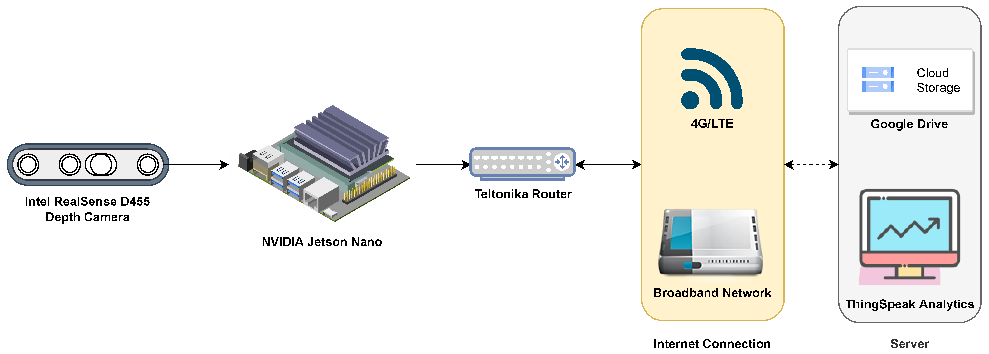
To effectively utilise edge computing, a processing powerhouse was required, ideally in a small form factor. The prototype was developed with the intention to be deployed in remote and rural areas. Therefore, the hardware setup was designed to achieve the utmost unsupervised automated operation in order to minimise physical site visits to perform maintenance or modification. As for the powerhouse for processing, a compact yet powerful NVIDIA Jetson Nano was used as the computing platform. For the RGB-D sensor, the Intel RealSense D455 was chosen as it could reliably provide both RGB and depth information through its on-board processing capabilities. The entire setup was connected to the Internet through a Teltonika industrial router, which provided a connection fail-over redundancy through a Long-Term Evolution (LTE) mobile network in case of disconnection from the main wired broadband network. Figure 6 displays the hardware topology.

The Intel RealSense D455 contains an in-body IR projector that allows depth perception in low-light situations, thus allowing the extraction of depth at night or in low-light conditions without additional hardware required. The camera was placed vertically below the platform and the electronics devices were housed in a weatherproof enclosure mounted on the platform. The physical setup of the computing platform, communication device and the RGB-D sensor are shown in Figure 7. The surface of the camera was parallel with the water surface as it provided the best viewing option of the water from the platform. Furthermore, whether the water level increased steadily or at a steep gradient towards the camera, the measurement accuracy increased, as it effectively shortened the distance between the camera sensors and the measuring object. The water gate itself housed a monitoring system which comprised ultrasonic sensors and a logging device. The data collected from this pre-existing system were used to verify the accuracy and reliability of the depth readings from the proposed system.

4.3. Bandwidth Measurements

Another important aspect of this study focused on the comparison of bandwidth consumption requirements of an edge computing device and a cloud computing device. To perform the same processing steps on the cloud as was performed on the edge device, raw and uncompressed data were required to be sent to the cloud. For this study, the uncompressed and unfiltered data, which were Robot Operating System (ROS) bag format files, were uploaded to Google Drive via its application programming interface (API) accessed through Python. On the other hand, the final processed depth readings were uploaded onto the ThingSpeak Analytics dashboard via the representational state transfer (REST) API. The consumption of bandwidth was measured accordingly as shown in the block diagram in Figure 8. The ROS file contained data required for the cloud server to process the depth readings, without which the depth extraction pipeline would not work on the cloud.

To measure the time taken and bytes uploaded, respectively, the program initialised a performance counter and recorded it, immediately followed by measuring the network input/output data prior to uploading the ROS file. As the data were successfully uploaded, the network input/output counter was recorded, and the second performance counter was recorded. The time taken to upload the data was the difference between the two performance counters and the total bytes uploaded were the difference between the two network input/output counters. The same methodology was applied to the data uploaded to the IoT analytics dashboard, which was processed on the Jetson Nano edge device.

5. Results and Analysis

The measurements were continuously taken over a 24 h period and divided into daylight hours (06:30–18:40) and night hours (18:40–6:30). The conditions during the measurements included clear skies, overcast and heavy precipitation. The measurement period was scattered over a few weeks to allow the system to be tested under diverse weather conditions.

During the initial stage of data collection, it was found that some of the images captured by the sensor were affected by sun glare. The issue was tackled by applying polarising filters on the stereo imagers to eliminate the reflection from the water surface. The results presented were collected from the setup with the polarising filter applied.

The testing results were compiled and analysed from two different angles. Firstly, the overall results (Figure 9, Figure 10, Figure 11 and Figure 12) were collectively analysed to understand the measurement performance during the daylight and night hours. The results in the graphs are segmented into day and night periods separated by the dashed line. Secondly, a separate analysis was performed on different scenarios to understand the effect of weather conditions on the measurement performance. Four sets of results in the form of graphs are presented in Figure 9, Figure 10, Figure 11 and Figure 12 where different weather conditions are depicted in different colour shades accordingly. The variation in weather provided a natural and automatic diversification of the testing dataset which tested the performance of the depth perception.

5.1. Daylight Readings

The daylight (morning) readings collected consisted of 101 data points and the water level ranged from below −2 m to above 2 m. The water level measurement was offset to match the pre-existing system which was calibrated against the mean sea level (MSL) during the construction of the water gate facility. The measurement data plots generated by the system against the ultrasonic sensor are shown in the figures below. The root-mean-square error (RMSE) during the daylight was 0.41 m averaged over the entire testing period. The breakdown of the RMSE for each weather condition for both day and night periods is tabulated in

Table 1. Collective RMSE error under all weather conditions.

	Cloudy	Fair	Rain
RMSE (day)	0.39 m	0.66 m	0.23 m
RMSE (night)	0.16 m	0.23 m	0.2 m
Data points (day)	57.84%	14.71%	27.45%
Data points (night)	38.6%	28.65%	32.75%

. Although the installation of the polariser significantly improved the stability and consistency of the results, the reflections appearing from different angles had the tendency to cause the camera to miscalculate the depth, resulting in a greater RMSE error during the day.

5.2. Night Readings

For the night readings, 172 data points were collected in total. The readings under the complete absence of visible light and external sources resulted in a root-mean-square error (RMSE) of 0.2 m, significantly lower than that of daylight measurements. The absence of reflections and wayward lights and the activation of infrared light during the night provided a much more stable and accurate reading. The breakdown of the weather conditions for the collected results throughout the testing phase is presented in Table 1.

The weather conditions varied constantly as the testing period progressed. During the dark hours, cloudy and fair weather conditions were indistinguishable, whereas fair during the daytime referred to clear skies with more sunlight exposure. To distinguish the different weather conditions, Weather Underground [47] was used to obtain historical data for each hour of the testing period. Since not all areas of a city experience the exact same weather, an error from mismatching the weather condition to its testing hour is possible. The results were segmented into different scenarios to better differentiate the conditions the system experienced in each period. Each testing period, the system experienced different weather conditions during different times of the day and night, and on multiple occasions throughout, the weather abruptly changed on-site.

We observed that the readings were smoother during the night, with tiny fluctuations around the ground-truth ultrasonic sensor data. As the day started, the deviations and fluctuations grew larger. Across the three weather conditions, as can be seen from the graphs and the tables, a fair weather provided the most erroneous readings, both during the day and night. The RMSE, however, was only marginally greater than in rainy weather during the night, while it was significantly greater during the day. Cloudy conditions also covered the occurrence of partial clouds over the water region, hence the possibility of partial illumination and partial shading of the water region, which contributed to the high RMSE during the day. The biggest factor contributing to the high RMSE during the day was occlusion and glare, resulting from the reflections of the sunlight hitting the camera sensor off the water surface.

Night readings showed a promising output which closely reflected the movement of the water level captured by the benchmarked ultrasonic sensor. On the contrary, clear skies during the day resulted in the largest RMSE, thus being responsible for a big percentage of the day’s large RMSE values. As the conditions became rainy and stormy, the readings became more accurate and resulted in the lowest RMSE during the day while being slightly more erroneous than the night readings. Nonetheless, when the rain poured down, the system captured depth accurately and consistently. The spatial filter continuously smoothened out the higher-frequency raindrops disturbing the water surface.

The case for complex illumination conditions can be made for daytime readings rather than night readings, as the presence of reflections and glare under cloudy and fair weather conditions proved to be challenging for the camera to tackle. It is also important to note that the measurement spots of the ultrasonic sensor and camera sensors were located some distance apart. This situation was also one of the potential sources of error due to the dynamic movement of the water flow throughout the stream, which might have led to differences in water level readings. Moreover, due to the limitation of the on-site camera placement, shadows formed on the water surface due to the reflection of the sky, rendering the readings erroneous. The limitations due to the structural formation of the platform and water gate placed the system’s depth readings at a slight disadvantage, especially during the daylight testing period.

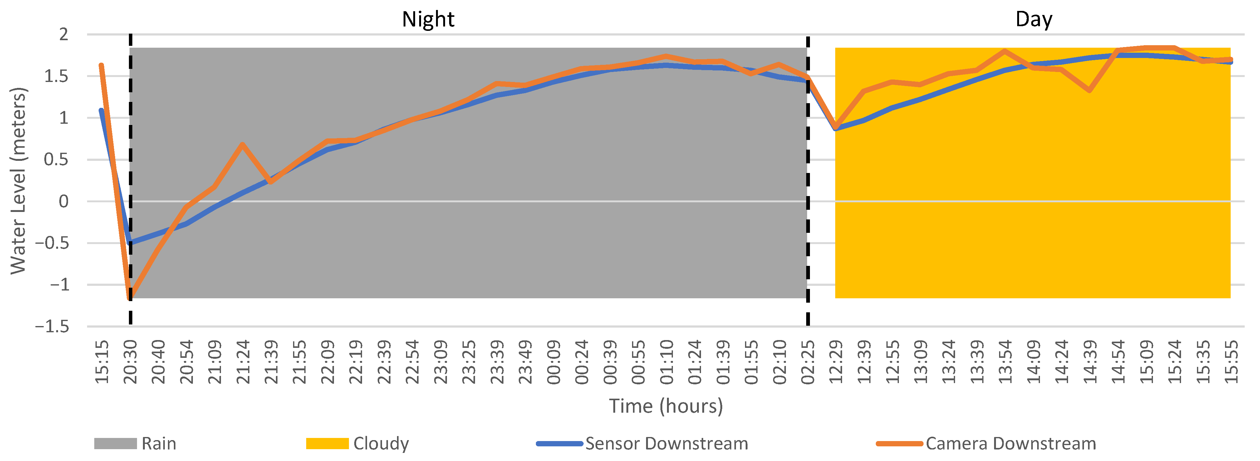
5.3. Scenario 1: Consistent Weather

Scenario 1 showcases the performance of the system under consistent weather conditions during each testing period, i.e., rainy during the night and cloudy during the day. The weather remaining consistent allowed the system readings to be stable as there was relatively little fluctuation in the readings across both periods. In this scenario, the day RMSE was 0.23 m while the night RMSE was slightly lower at 0.2 m.

5.4. Scenario 2: Slight Fluctuations in Weather

The system experienced some weather fluctuations in scenario 2, although all the fluctuations occurred during the night and none during the day period. Even with the fluctuation in weather condition, the system RMSE during the night was the lowest under this scenario, while during the day readings it was the highest. Even with the fluctuations in weather conditions, the system RMSE was 0.18 m, the lowest night-reading RMSE across all scenarios. On the contrary, the system RMSE during the day was 0.51 m, the highest during the day periods across the testing period.

5.5. Scenario 3: Normal Fluctuations in Weather

The system experienced a moderate amount of weather fluctuations, slightly more than in scenario 2. Scenario 3’s monitoring period also extended longer than each of the previous two scenarios. Similar to scenario 2, the weather fluctuated multiple times during the night while during the day, it changed once from cloudy to rainy halfway during the day. The readings were most erroneous during the day when it was cloudy and much more stable when raining. Under this scenario, the system RMSE during the day was 0.33 m while during the night, the system RMSE was 0.2 m, one of the lowest across the entire testing period.

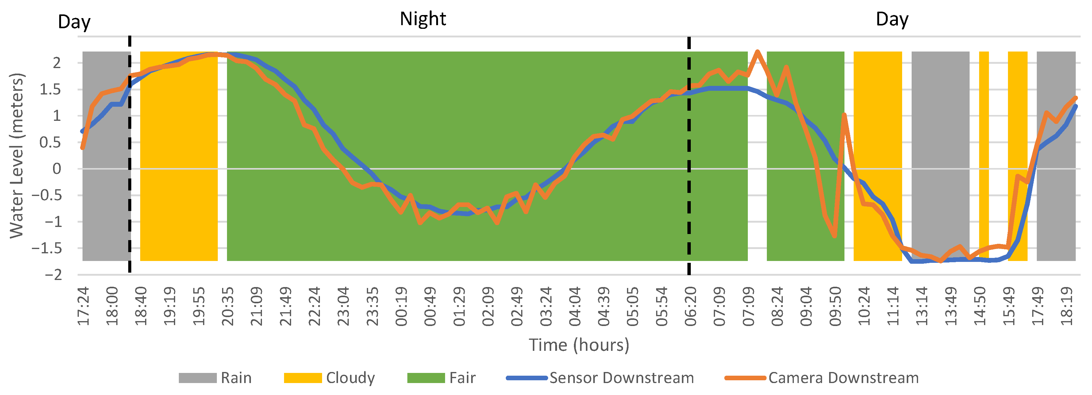
5.6. Scenario 4: Frequent Fluctuations in Weather

In scenario 4, the system experienced weather fluctuations more frequently and abruptly than the previous three scenarios. The weather fluctuated between all the three main categories during both testing periods. Most of the night period was fair, meaning clear skies, and that was also the most erroneous the readings were amongst all four scenarios as the system RMSE was 0.21 m. During the day, it fell within the category of one of the highest RMSEs at 0.48 m.

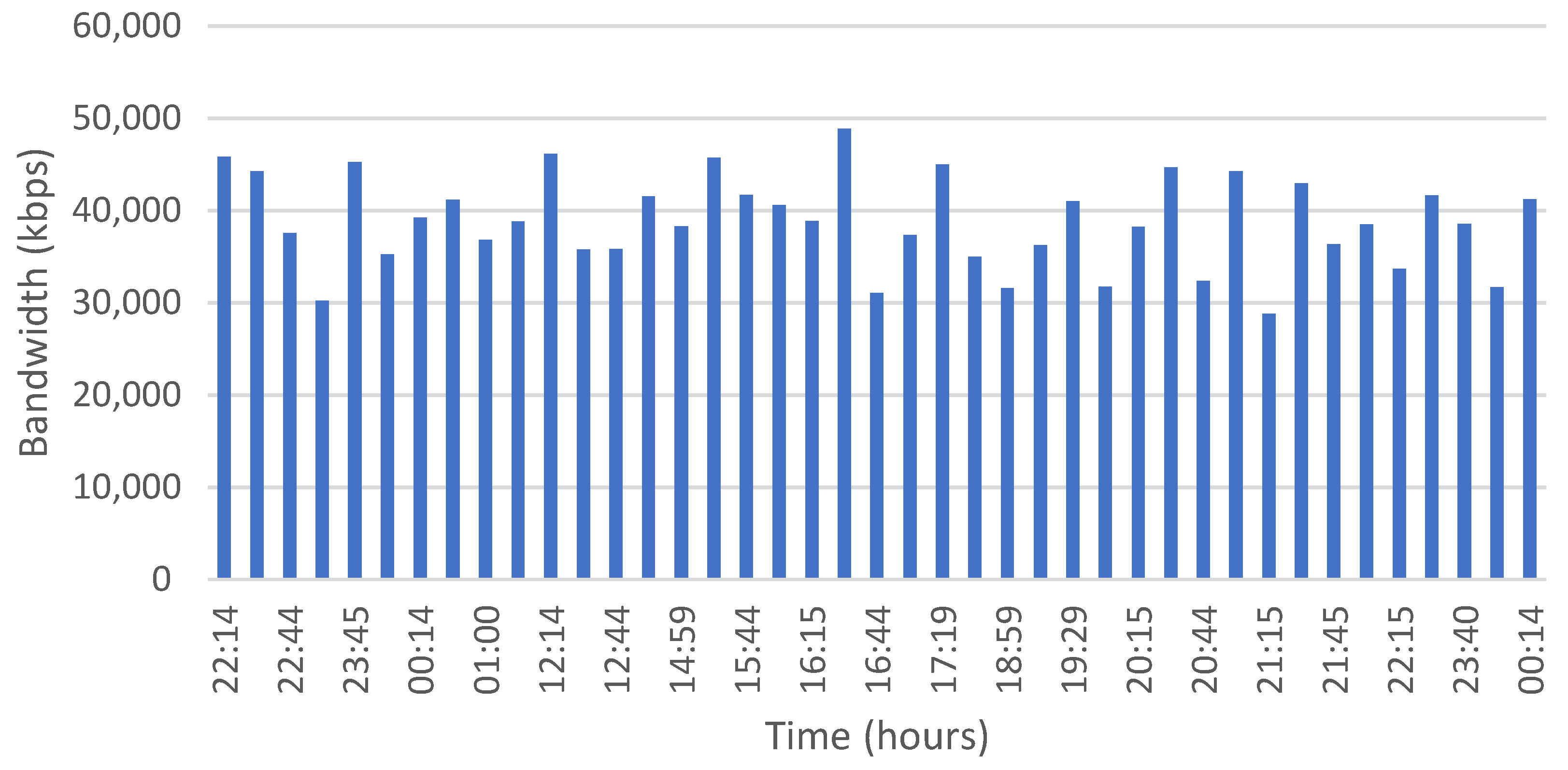
5.7. Bandwidth Consumption

During the experimental period, an evaluation of the bandwidth usage was also conducted in order to compare the bandwidth requirements between cloud-based and edge-based processing technique. The total bandwidth consumed over the course of a single testing day for both computing models are presented in Figure 13 and Figure 14. The bandwidth capacity required for uploading the data to the cloud was approximately 50,000 kilobits per second (Kbps) whereas uploading processed edge information to the dashboard maxed out at just over 12 Kbps.

The results demonstrated the difference in bandwidth consumed for each of the computing strategies; the edge computing strategy proved to be more bandwidth efficient. The total data usage to upload edge data to the dashboard over a 24 h period was approximately 0.92 Mb whereas it took 11,106 Mb to upload raw data to cloud storage. The experiment showed that uploading uncompressed information to the cloud required approximately 12,072 times more data usage than uploading the processed data to the cloud dashboard. There was a massive data and bandwidth reduction in the edge pipeline, especially when the application involved real-time monitoring using image and video data. By utilising edge computing, the bandwidth consumption was greatly reduced thus alleviating stress off the network [48]. This is beneficial for installing real-time monitoring applications in rural areas where network bandwidth is a major concern for IoT devices.

6. Conclusions and Future Work

In this paper, we proposed, designed, implemented and deployed a novel real-time flood monitoring system driven by computer vision, edge computing and an IoT system architecture. We used RealSense D455’s stereo vision capabilities to extract depth from a complex medium such as water, which provided great insights into the application of RGB-D cameras in flood monitoring. The RGB-D camera was integrated with an edge computing device (Jetson Nano), to continuously process and log all critical incoming RGB-D image sensor data. The performance of the deployed system was analysed and compared with calibrated specialised ultrasonic sensor data. The system was deployed and tested under a variety of weather and lighting conditions in an actual flood mitigation facility.

The experimental results demonstrated the promising potential of using the proposed solution to perform water level measurement using a computer-vision-based sensor. Results obtained during the night highlighted the stereoscopic capabilities of the RealSense D455, where it performed well under no visible lighting. Furthermore, running the prototype throughout the experimental period of more than 24 weeks demonstrated the reliability and capability of the proposed system. The implementation of a real-time flood monitoring system at the edge demonstrated the potential and benefits of installing similar systems in resource-constrained environments and without external measurement guide or additional hardware.

Future work will investigate combining and superimposing RGB images, artefacts and cues onto depth maps to improve the overall accuracy and reliability of the system. To enable the system to be more dynamic and applicable at any water site, the incorporation of the internal inertial measurement unit (IMU) readings of the camera and frame subtraction techniques will be investigated. Our work can serve as a reference and further be expanded into different application domains, such as those in smart cities and smart manufacturing. For instance, the images captured by the image sensor could be used to detect illegal intrusion or vandalism attempt around the facility. Images and footage from multiple stereoscopic cameras at the same location could be utilised for sensor fusion. Additional stereoscopic depth cameras may be useful in providing information over a larger area and assist in differentiating among errors during various operational conditions, which may potentially be advantageous. Image information could also be used to detect river pollution or illegal dumping activities along the river streams which would be advantageous to the relevant authorities insofar as taking pre-emptive action for containing the effect of the pollution.

References

- Dib, A.; Estcourt, D. Victoria Floods: Power Outages Continue across State as Extreme Weather Cleanup Begins. Available online: https://www.theage.com.au/national/victoria/about-24-000-still-without-power-as-victoria-s-storm-recovery-continues-20210614-p580s4.html (accessed on 16 June 2022).
- Beers, L.M. Wild Weather Smashes Victoria with Roads Closed, Flash Flooding and Power Outages. Available online: https://7news.com.au/weather/melbourne-weather/wild-weather-smashes-victoria-with-roads-closed-trees-down-and-flash-flooding-c-3067406 (accessed on 16 June 2022).
- Arshad, B.; Ogie, R.; Barthelemy, J.; Pradhan, B.; Verstaevel, N.; Perez, P. Computer Vision and IoT-Based Sensors in Flood Monitoring and Mapping: A Systematic Review. Sensors 2019, 19, 5012. [Google Scholar] [CrossRef] [PubMed]
- Mitra, A.; Biswas, S.; Adhikari, T.; Ghosh, A.; De, S.; Karmakar, R. Emergence of Edge Computing: An Advancement over Cloud and Fog. In Proceedings of the 2020 11th International Conference on Computing, Communication and Networking Technologies (ICCCNT), Kharagpur, India, 1–3 July 2020; pp. 1–7. [Google Scholar] [CrossRef]
- Baller, S.P.; Jindal, A.; Chadha, M.; Gerndt, M. DeepEdgeBench: Benchmarking Deep Neural Networks on Edge Devices. In Proceedings of the 2021 IEEE International Conference on Cloud Engineering (IC2E), San Francisco, CA, USA, 4–8 October 2021; pp. 20–30. [Google Scholar]
- Hajder, P.; Rauch, Ł. Moving Multiscale Modelling to the Edge: Benchmarking and Load Optimization for Cellular Automata on Low Power Microcomputers. Processes 2021, 9, 2225. [Google Scholar] [CrossRef]
- Yu, W.; Liang, F.; He, X.; Hatcher, W.G.; Lu, C.; Lin, J.; Yang, X. A survey on the edge computing for the Internet of Things. IEEE Access 2017, 6, 6900–6919. [Google Scholar] [CrossRef]
- Kua, J.; Armitage, G.; Branch, P. A Survey of Rate Adaptation Techniques for Dynamic Adaptive Streaming Over HTTP. IEEE Commun. Surv. Tutorials 2017, 19, 1842–1866. [Google Scholar] [CrossRef]
- Kua, J.; Loke, S.W.; Arora, C.; Fernando, N.; Ranaweera, C. Internet of things in space: A review of opportunities and challenges from satellite-aided computing to digitally-enhanced space living. Sensors 2021, 21, 8117. [Google Scholar] [CrossRef]
- Leduc, P.; Ashmore, P.; Sjogren, D. Technical note: Stage and water width measurement of a mountain stream using a simple time-lapse camera. Hydrol. Earth Syst. Sci. 2018, 22, 1–11. [Google Scholar] [CrossRef]
- Kua, J.; Armitage, G.; Branch, P.; However, J. Adaptive Chunklets and AQM for Higher-Performance Content Streaming. ACM Trans. Multimed. Comput. Commun. Appl. 2019, 15, 1–24. [Google Scholar] [CrossRef]
- Kua, J.; Armitage, G. Optimising DASH over AQM-Enabled Gateways Using Intra-Chunk Parallel Retrieval (Chunklets). In Proceedings of the 2017 26th International Conference on Computer Communication and Networks (ICCCN), Vancouver, BC, Canada, 31 July–3 August 2017; pp. 1–9. [Google Scholar] [CrossRef]
- Kua, J.; Armitage, G.; Branch, P. The Impact of Active Queue Management on DASH-Based Content Delivery. In Proceedings of the 2016 IEEE 41st Conference on Local Computer Networks (LCN), Dubai, United Arab Emirates, 7–10 November 2016; pp. 121–128. [Google Scholar] [CrossRef]
- Kua, J.; Armitage, G. Generating Dynamic Adaptive Streaming over HTTP Traffic Flows with TEACUP Testbed; Tech. Rep. A; Centre for Advanced Internet Architectures, Swinburne University of Technology: Melbourne, Australia, 2016; Volume 161216, p. 16. [Google Scholar]
- Kua, J.; Nguyen, S.H.; Armitage, G.; Branch, P. Using Active Queue Management to Assist IoT Application Flows in Home Broadband Networks. IEEE Internet Things J. 2017, 4, 1399–1407. [Google Scholar] [CrossRef]
- Kua, J.; Branch, P.; Armitage, G. Detecting bottleneck use of pie or fq-codel active queue management during dash-like content streaming. In Proceedings of the 2020 IEEE 45th Conference on Local Computer Networks (LCN), Sydney, NSW, Australia, 16–19 November 2020; pp. 445–448. [Google Scholar]
- Kua, J. Understanding the Achieved Rate Multiplication Effect in FlowQueue-based AQM Bottleneck. In Proceedings of the 2021 IEEE 46th Conference on Local Computer Networks (LCN), Edmonton, AB, Canada, 4–7 October 2021; pp. 439–442. [Google Scholar]
- Kua, J.; Al-Saadi, R.; Armitage, G. Using Dummynet AQM-FreeBSD’s CoDel, PIE, FQ-CoDel and FQ-PIE with TEACUP v1.0 Testbed; Tech. Rep. A; Centre for Advanced Internet Architectures, Swinburne University of Technology: Melbourne, Australia, 2016; Volume 160708, p. 8. [Google Scholar]
- Zhang, Z.; Zhou, Y.; Liu, H.; Gao, H. In-situ water level measurement using NIR-imaging video camera. Flow Meas. Instrum. 2019, 67, 95–106. [Google Scholar] [CrossRef]
- Bruinink, M.; Chandarr, A.; Rudinac, M.; van Overloop, P.J.; Jonker, P. Portable, automatic water level estimation using mobile phone cameras. In Proceedings of the 2015 14th IAPR international conference on Machine Vision Applications (MVA), Tokyo, Japan, 18–22 May 2015; pp. 426–429. [Google Scholar]
- Kim, Y.; Park, H.; Lee, C.; Kim, D.; Seo, M. Development of a cloud-based image water level gauge. IT Converg. Pract. (INPRA) 2014, 2, 22–29. [Google Scholar]
- Lin, Y.T.; Lin, Y.C.; Han, J.Y. Automatic water-level detection using single-camera images with varied poses. Measurement 2018, 127, 167–174. [Google Scholar] [CrossRef]
- Hough, P.V. Method and Means for Recognizing Complex Patterns. U.S. Patent 3,069,654, 18 December 1962. [Google Scholar]
- Ortigossa, E.S.; Dias, F.; Ueyama, J.; Nonato, L.G. Using digital image processing to estimate the depth of urban streams. In Proceedings of the Workshop of Undergraduate Works in Conjunction with Conference on Graphics, Patterns and Images (SIBGRAPI), Bahia, Brazil, 26–29 August 2015; pp. 26–29. [Google Scholar]
- Li, H.P.; Wang, W.; Ma, F.C.; Liu, H.L.; Lv, T. The water level automatic measurement technology based on image processing. In Applied Mechanics and Materials; Trans Tech Publ.: Bäch SZ, Switzerland, 2013; Volume 303, pp. 621–626. [Google Scholar]
- Zhang, Z.; Zhou, Y.; Liu, H.; Zhang, L.; Wang, H. Visual Measurement of Water Level under Complex Illumination Conditions. Sensors 2019, 19, 4141. [Google Scholar] [CrossRef] [PubMed]
- Otsu, N. A Threshold Selection Method from Gray-Level Histograms. IEEE Trans. Syst. Man Cybern. 1979, 9, 62–66. [Google Scholar] [CrossRef]
- Ren, H.; Gao, N.; Li, J. Monocular Depth Estimation with Traditional Stereo Matching Information. In Proceedings of the 2019 6th International Conference on Systems and Informatics (ICSAI), Shanghai, China, 2–4 November 2019; pp. 1319–1323. [Google Scholar]
- Xian, K.; Shen, C.; Cao, Z.; Lu, H.; Xiao, Y.; Li, R.; Luo, Z. Monocular relative depth perception with web stereo data supervision. In Proceedings of the IEEE Conference on Computer Vision and Pattern Recognition, Salt Lake City, UT, USA, 18–23 June 2018; pp. 311–320. [Google Scholar]
- Pan, J.; Yin, Y.; Xiong, J.; Luo, W.; Gui, G.; Sari, H. Deep Learning-Based Unmanned Surveillance Systems for Observing Water Levels. IEEE Access 2018, 6, 73561–73571. [Google Scholar] [CrossRef]
- Jafari, N.H.; Li, X.; Chen, Q.; Le, C.Y.; Betzer, L.P.; Liang, Y. Real-time water level monitoring using live cameras and computer vision techniques. Comput. Geosci. 2021, 147, 104642. [Google Scholar] [CrossRef]
- Bung, D.B.; Crookston, B.M.; Valero, D. Turbulent free-surface monitoring with an RGB-D sensor: The hydraulic jump case. J. Hydraul. Res. 2021, 59, 779–790. [Google Scholar] [CrossRef]
- Bi, Y.; Li, J.; Qin, H.; Lan, M.; Shan, M.; Lin, F.; Chen, B.M. An MAV Localization and Mapping System Based on Dual Realsense Cameras. In Proceedings of the 2016 International Micro Air Vehicle Conference and Competition, Beijing, China, 17–21 October 2016; pp. 50–55. [Google Scholar]
- Chen, Y.C.; Weng, W.C.; Lin, S.W. A High Reliability 3D Object Tracking Method for Robot Teaching Application. In IOP Conference Series: Materials Science and Engineering; IOP Publishing: Bristol, UK, 2019; Volume 644. [Google Scholar]
- Wegner, P. Global IoT Market Size Grew 22% in 2021. Available online: https://iot-analytics.com/iot-market-size/ (accessed on 16 June 2022).
- Atzori, L.; Iera, A.; Morabito, G. The internet of things: A survey. Comput. Netw. 2010, 54, 2787–2805. [Google Scholar] [CrossRef]
- Li, S.; Xu, L.D.; Zhao, S. The internet of things: A survey. Inf. Syst. Front. 2015, 17, 243–259. [Google Scholar] [CrossRef]
- Al-Fuqaha, A.; Guizani, M.; Mohammadi, M.; Aledhari, M.; Ayyash, M. Internet of things: A survey on enabling technologies, protocols, and applications. IEEE Commun. Surv. Tutorials 2015, 17, 2347–2376. [Google Scholar] [CrossRef]
- Ai, Y.; Peng, M.; Zhang, K. Edge computing technologies for Internet of Things: A primer. Digital Commun. Netw. 2018, 4, 77–86. [Google Scholar] [CrossRef]
- Pan, J.; McElhannon, J. Future edge cloud and edge computing for internet of things applications. IEEE Internet Things J. 2017, 5, 439–449. [Google Scholar] [CrossRef]
- Premsankar, G.; Di Francesco, M.; Taleb, T. Edge computing for the Internet of Things: A case study. IEEE Internet Things J. 2018, 5, 1275–1284. [Google Scholar] [CrossRef]
- Intel® RealSense™ Depth Camera D455. Available online: https://www.intelrealsense.com/depth-camera-d455/ (accessed on 22 October 2022).
- Keselman, L.; Iselin Woodfill, J.; Grunnet-Jepsen, A.; Bhowmik, A. Intel(R) RealSense(TM) Stereoscopic Depth Cameras. In Proceedings of the 2017 IEEE Conference on Computer Vision and Pattern Recognition Workshops (CVPRW), Honolulu, HI, USA, 21–26 July 2017; pp. 1267–1276. [Google Scholar] [CrossRef]
- Grunnet-Jepsen, A.; Tong, D. Depth Post-Processing FOR Intel® REALSENSE™ Depth Camera D400 Series. Available online: https://dev.intelrealsense.com/docs/depth-post-processing (accessed on 1 August 2022).
- Ngan, K.N. Experiments on two-dimensional decimation in time and orthogonal transform domains. Signal Process. 1986, 11, 249–263. [Google Scholar] [CrossRef]
- Crochiere, R.; Rabiner, L. Interpolation and decimation of digital signals—A tutorial review. Proc. IEEE 1981, 69, 300–331. [Google Scholar] [CrossRef]
- Kuching, Malaysia Weather History. Available online: https://www.wunderground.com/history/daily/my/kuching/WBGG (accessed on 18 April 2022).
- Das, A.; Patterson, S.; Wittie, M. EdgeBench: Benchmarking Edge Computing Platforms. In Proceedings of the 2018 IEEE/ACM International Conference on Utility and Cloud Computing Companion (UCC Companion), Zurich, Switzerland, 17–20 December 2018; pp. 175–180. [Google Scholar] [CrossRef]