1. Introduction
Headwater catchments bring together complex environmental gradients, vegetation patches, soils, and biological processes that occur in proximity. In forested, mountain landscapes, functions such as carbon storage, biomass production, soil development, erosion regulation, deadwood accumulation, and plant diversity are not controlled by a single factor. Rather, they respond to climate, topography, forest structure, soil conditions, and disturbance, often at the same time. This is especially relevant in western Patagonia, where steep climatic gradients, large temperate forests, and increasing human pressures occur in still relatively intact mountain watersheds [
1,
2,
3,
4]. Even so, field-based assessments that account for multiple ecosystem functions in an integrated manner are still scarce in this region [
5].
Ecosystems perform many functions at the same time. Because of this, the condition of one function is not enough to infer how the whole system is working [
6,
7,
8]. In forests, carbon storage, biomass production, nutrient cycling, soil processes, and biodiversity may respond according to differing forest structures, composition, diversity, and environmental contexts [
9,
10,
11,
12,
13]. As a result, a high value in one function can co-occur with high values in other functions (i.e., synergy), but it can also occur with losses in other parts of the system (i.e., trade-off) [
8]. In western Patagonia, a recent spatial analysis found synergies among carbon storage, nutrient availability, and other mapped functions [
14]. These results show that multiple functions need to be analyzed together to better understand how these landscapes are organized and interact.
Interactions among ecosystem functions can have different causal mechanisms. Two functions may be directly linked, but they can also look connected because both functions respond to the same environmental or human driver [
15,
16]. Simple pairwise correlations cannot separate these two possibilities. Unlike separate regression models fitted independently for each ecosystem function, Bayesian networks represent the joint conditional structure of multiple functions and drivers within a single graphical model. They can therefore make a driver-mediated relationship look like a direct trade-off or synergy [
17,
18]. This distinction is important for management. If two functions respond to the same driver, acting on that driver may change both functions. If the relationship is direct, then acting on one function may have a different effect. Disturbance adds another layer of complexity. It often reduces carbon storage and several regulating functions, but its effect on biodiversity can be positive or negative depending on disturbance type, intensity, legacy, and local context [
19,
20,
21].
The scale of observation can also change what we measure, interpret and monitor. Plot-level data capture local variation in vegetation, soils, and disturbance history, but larger-scale analysis units, such as forest clusters or catchments, integrate more environmental heterogeneity and landscape composition [
22]. For this reason, the strength and even the direction of trade-offs and synergies can change across spatial scales [
23,
24]. This is especially important in mountain landscapes, where plots are nested within forest stands, catchments, and regional climatic gradients [
2]. However, forest multifunctionality studies are still geographically concentrated, and many assessments do not fully represent the links among aboveground, belowground, structural, and environmental drivers [
12]. Many multiscale studies also rely on mapped or modeled indicators rather than on nested field measurements [
14,
22,
23].
Accordingly, Bayesian networks are useful for understanding such problems because they can represent conditional relationships among functions and drivers while also including ecological restrictions and uncertainty [
25,
26,
27]. They have been used to study trade-offs, synergies, scenarios, and relationships mediated by shared drivers [
18,
28]. Their graphical structure also helps to communicate complex systems [
27]. However, their structure depends on the variables included, the drivers that may be missing, the prior restrictions, and the scale of the data. Learned links should therefore not be read automatically as causal relationships [
29]. This is especially important when sample size changes among scales, as happens in nested field designs.
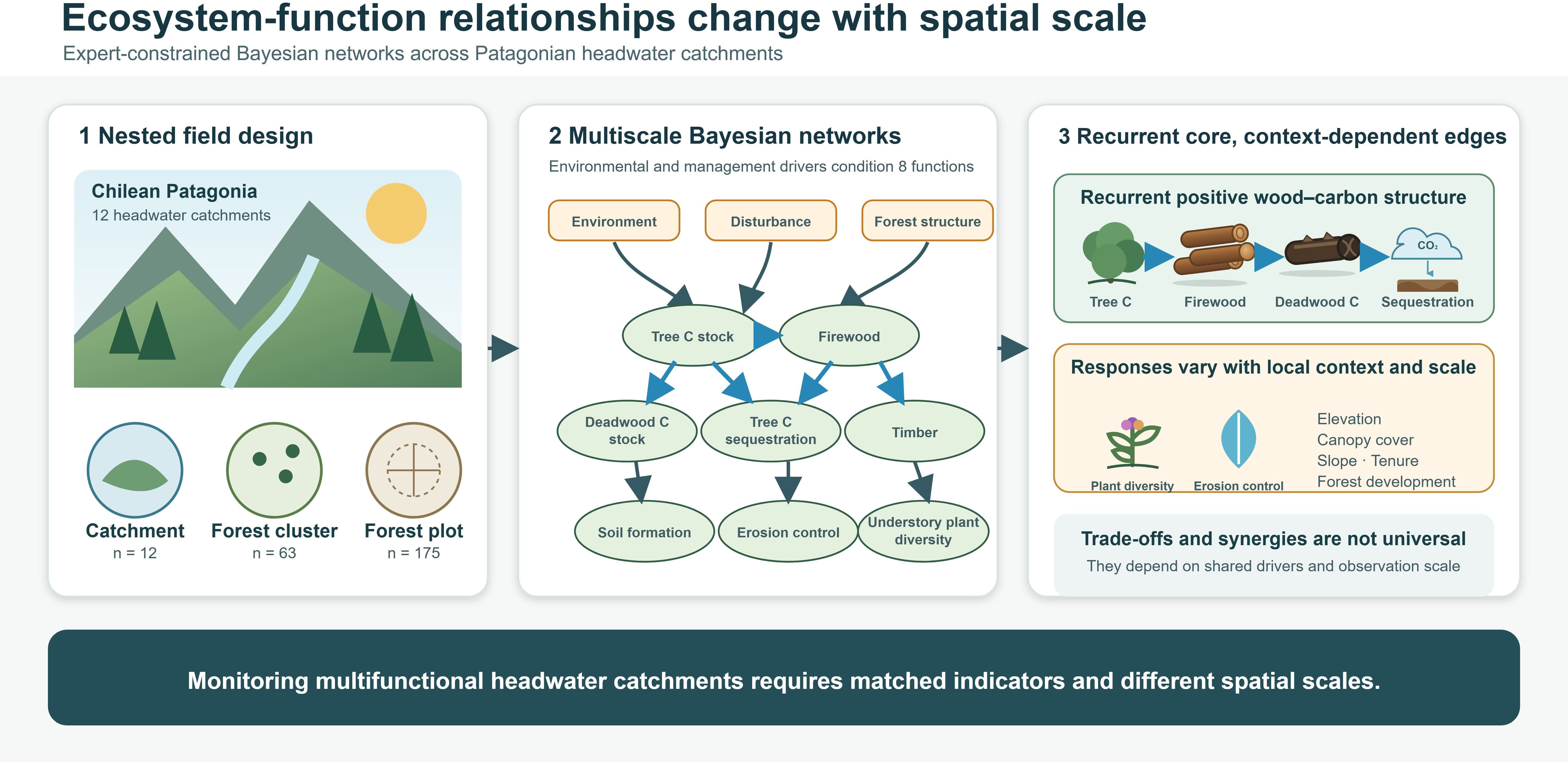
Here, we aimed to: determine how environmental conditions, disturbance, and observational scale shape the relationships among ecosystem functions in twelve headwater catchments of the Aysén Region, Chilean Patagonia. We used a systematic nested field inventory that measured forest, soil, and biodiversity-related functions at three complementary scales: catchment, forest cluster, and plot [
5]. The analytical framework consisted of three corresponding Bayesian network models. The catchment-scale model provided a constrained synthesis of broad climatic and disturbance-related patterns; the forest-cluster model evaluated relationships among functions and drivers at the stand scale; and the plot-level model was used as a sensitivity analysis to determine which relationships persisted or changed when local variation was retained. We tested three working hypotheses: (H1) accounting for shared environmental and disturbance drivers would reduce the number of apparent direct relationships among ecosystem functions; (H2) tree carbon stock, wood-production, and soil-related functions would form a recurrent positive functional structure, whereas carbon sequestration could partly decouple from accumulated carbon stocks; and (H3) disturbance would generally reduce carbon storage and soil-regulation functions, whereas biodiversity responses and the strength and direction of relationships among functions would vary with environmental context and spatial scale.
2. Materials and Methods
2.1. Study Area and Sampling Design
The study was conducted in headwater catchments of the Aysén and Baker River basins in southwestern Patagonia in Chile (46–47° S). This region has a strong dry-to-wet climatic gradient that is also expressed in its forest composition. Eastern semi-arid sites are closer to cold steppe and deciduous southern beech forests dominated by
Nothofagus antarctica and
N. pumilio. Further west, humid forests include evergreen and mixed assemblages with
N. nitida,
N. betuloides,
N. dombeyi,
Drimys winteri, and
Laureliopsis philippiana [
30]. Soils are mainly volcanic, especially andosols with different textures and degrees of development, over poorly weathered granitic or basaltic bedrock and some unconsolidated Quaternary deposits [
31,
32,
33].
The study followed an observational comparative design (
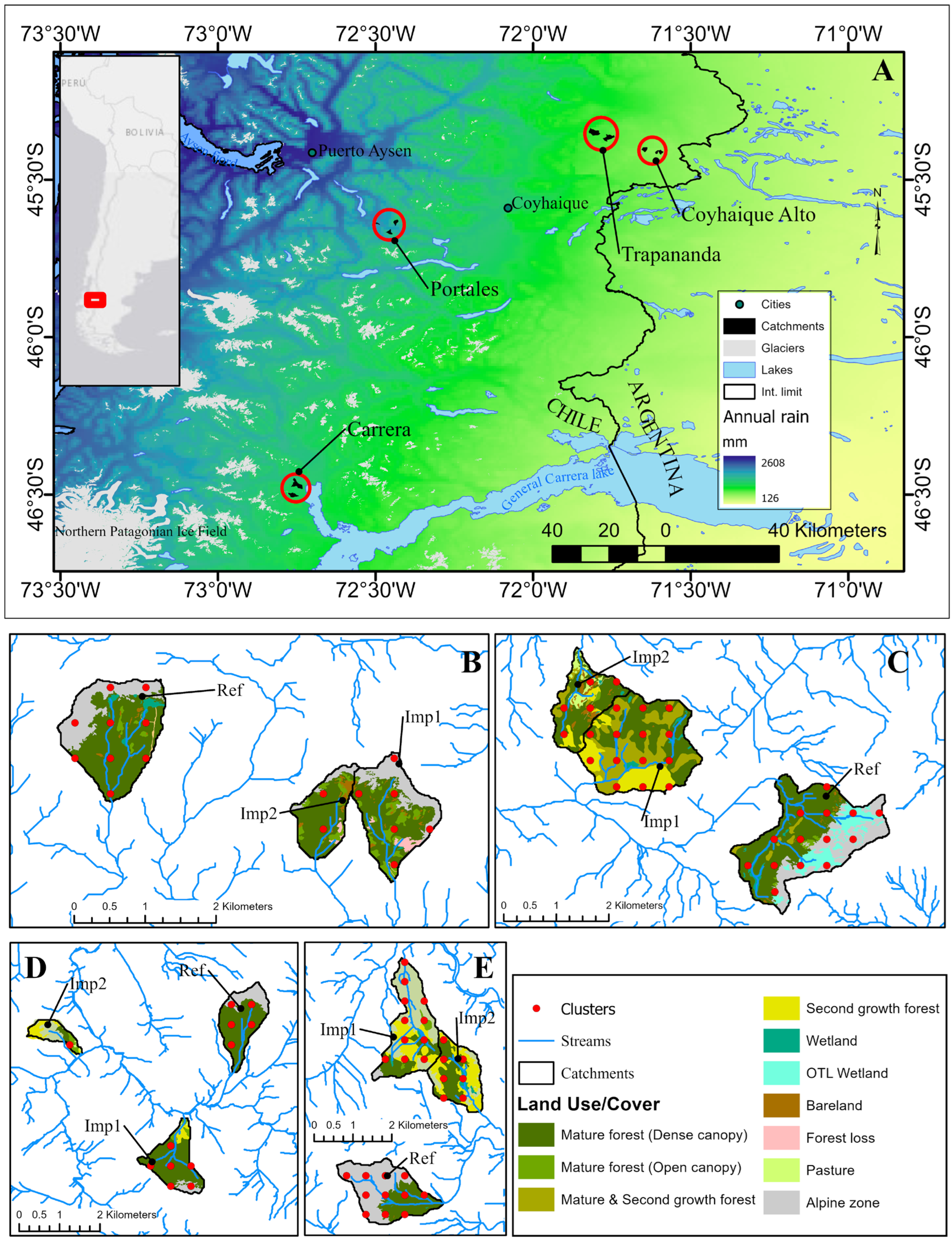
Figure A1). A total of 12 forested headwater catchments were selected across two climatic contexts (Ecosystem: Dry and Humid) and different land-use legacies (Treatment: Reference and Impacted) [
5]. The basic landscape units were first-order perennial streams with catchments ranging from 0.5 to 2.8 km
2 (
Table 1). Within each climatic context, catchments were chosen to be as comparable as possible in size, elevation, aspect, and slope, but different in disturbance history. At each site, three nearby catchments were selected: one reference catchment with low human influence and two impacted catchments with evidence of recent land-clearing fires, selective harvesting, and livestock grazing. Two dry sites were selected, Coyhaique Alto and Trapananda, and two humid sites, Portales and Carrera. Dry sites were higher, close to 1000 m a.s.l., within deciduous forest zones and with lower precipitation (approximately 500–900 mm yr
−1). Humid sites were lower, around 300–600 m a.s.l. and had higher precipitation (approximately 1500–2200 mm yr
−1).
The inventory used a systematic cluster-based design. Here, “cluster” refers to a predefined spatial sampling unit and not to a group obtained through statistical clustering. Each sampling cluster contained up to three 500 m
2 forest plots and an associated 50 m linear transect. To address the objectives of this study, we used three nested analytical levels: catchments, forest clusters, and forest plots. The catchment model used the full systematic inventory aggregated to the twelve catchments. The forest-cluster and plot-level models were restricted to forest stands because timber volume, firewood volume, deadwood carbon, and the exposed-root erosion proxy only have a clear ecological interpretation in this land use. A full description of the study area and sampling design is provided in Moreno-Meynard [
5].
2.2. Data Sources and Variable Reconstruction
Tree carbon stock, tree carbon sequestration, timber volume, firewood volume, soil formation, and soil erosion were reconstructed from plot-level components in Moreno-Meynard [
5]. Tree carbon stock and tree carbon sequestration were set to zero where no trees were present but the plot was evaluated. Timber and firewood volumes were assigned structural zeros only when the forest component had been evaluated and no stems meeting the corresponding product criteria were present. These zeros therefore represent an observed absence of the function rather than missing information; observations without a valid assessment were retained as missing. Soil formation was kept as measured volume per area, with true missing measurements left as missing before aggregation. Soil erosion was based on the exposed-root proxy [
34] and was used only where the proxy was applicable (forest plots). Although this indicator is a local proxy of cumulative soil loss around trees and does not capture all erosion processes or directly estimate contemporary erosion rates, it provided a rapid, field-based, and literature-supported method for incorporating erosion-related soil regulation into the systematic assessment of forest plots. Besides, for visualization, it was inverted and plotted as erosion control (1—normalized soil erosion).
The cluster-level deadwood carbon stock came from the Ecosystem_functions_by_cluster dataset in Moreno-Meynard [
5]. Plot-level deadwood carbon was reconstructed as the sum of the cluster downed-deadwood component and the plot standing-deadwood component, following the structure of the original published scripts (
Supplementary Material). Understory plant richness (hereafter, vascular richness) was treated as cluster-level richness at the catchment and forest-cluster scales. At the plot scale, it was calculated as the number of unique vascular plant species per plot.
Forest development stage was built from tree-level structure using quadratic mean diameter, maximum diameter, live tree count, and dead tree share. Plots were classified as sapling, secondary growth, adult forest, and old growth. This variable was included because forest structural development can organize carbon storage, deadwood accumulation, timber volume, and biodiversity in ways that are not captured by Treatment alone. Elevation was recorded in meters above sea level, slope as percentage inclination, and canopy cover was measured in the field using a densiometer and expressed as percentage cover. Aspect described the cardinal orientation of each plot; at the sampling-cluster scale, south aspect share was calculated as the proportion of forest plots with southern exposure. Impact type described the disturbance agents recorded in the field, including fire, forest harvesting, and livestock use, either individually or in combination. Impact level described the observed disturbance intensity using the categories no impact, low, medium, and high. These variables were obtained from Moreno-Meynard [
5] and used at the plot level when available. For the sampling-cluster model, continuous variables were averaged across the contributing forest plots, categorical variables were represented by their modal category, and southern exposure was retained as the proportion of south-facing plots. Following Moreno-Meynard [
5], tenure (ownership) was classified into four categories representing typical Patagonian land-tenure contexts: small landowner, large landowner, national park, and other public land.
2.3. Variables Used in Each Model
The ecosystem-function set was defined before fitting the Bayesian networks through a literature-guided selection of functions commonly considered in forest ecosystem-function and multifunctionality assessments. This initial selection was then constrained by the variables supported by the published field database and by the requirement that each function could be reconstructed with a consistent ecological interpretation at the catchment, sampling-cluster, and plot scales. The final common set comprised tree carbon stock, tree carbon sequestration, deadwood carbon stock, timber volume, firewood volume, soil formation, soil erosion, and vascular plant richness. Together, these functions represent complementary dimensions of carbon storage and dynamics, wood production, soil processes, and biodiversity. For Model 1, the unit of analysis was the catchment scale (0.5 to 2.8 km2, n = 12). Cluster-level values were averaged within each catchment using the systematic clusters belonging to that catchment. Non-forest clusters were retained where a function could be assigned a structural zero. Model 1 used ecosystem context (Humid = 0, Dry = 1), treatment (Reference = 0, Impacted = 1), and the eight common ecosystem-function nodes.
For Model 2, the unit of analysis was the forest-cluster scale (1500 m2 + 50 m linear transect). The final model used 63 forest clusters. The dataset included the eight common ecosystem-function nodes plus ecosystem context, elevation, slope, canopy cover, south aspect share, forest development stage, impact type, impact level, and ownership. Treatment was not considered in the final version of Model 2 because impact type and impact level gave a more explicit disturbance description. Slope, canopy cover, impact type, impact level, and ownership were summarized (mean or mode) from plot-level information to the cluster level. South aspect was kept as the share of forest plots with southern exposure.
For Model 3, the unit of analysis was the forest-plot scale (500 m2). The final model used 175 forest plots. The dataset included the same ecosystem-function nodes and covariates used in the cluster-level model. Because plots are nested within clusters, this model was interpreted as a plot-level sensitivity analysis and not as a fully independent landscape-level model.
2.4. Transformations and Bayesian Network Fitting
Bayesian networks were used to represent conditional dependencies among ecosystem functions and their environmental or disturbance-related predictors. Network structures were learned with the hill-climbing algorithm implemented in the bnlearn R package. Each model used 500 bootstrap replicates to estimate arc strength. The final averaged networks retained arcs using the model-specific threshold estimated from the bootstrap strength object.
Model 1 used log-transformed response nodes before structure learning. Ecosystem-function nodes were prevented from pointing into ecosystem or treatment. Three additional directions were also prohibited because they were ecologically unsupported in the final model definition: vascular richness to deadwood carbon stock, soil erosion to timber volume, and soil erosion to tree carbon sequestration. The arc from vascular richness to deadwood carbon stock was prohibited because contemporary understory richness was not considered a plausible upstream determinant of an accumulated structural stock governed primarily by tree mortality, decomposition, and stand history. The opposite direction remained available to the structure-learning algorithm.
Model 2 used the forest-cluster level. Response nodes were first transformed using log(x + 1), and numeric covariates were subsequently standardized to zero mean and unit variance. Ecosystem, elevation, slope, canopy cover, south aspect share, forest development stage, impact type, impact level, and ownership were treated as candidate predictor nodes. The structural blacklist prohibited all arcs ending in predictor nodes. Prohibiting arcs ending in these nodes reduced implausible feedback directions and improved model identifiability, without implying causal relationships or excluding possible ecological feedbacks over longer timescales.
Model 3 used the complete forest-plot level. Response nodes were first transformed using log(x + 1), and numeric covariates were subsequently standardized to zero mean and unit variance. Ecosystem, aspect, impact type, impact level, land use, ownership, forest development stage, slope, elevation, and canopy cover were treated as candidate predictor nodes. The structural blacklist prohibited all arcs ending in predictor nodes, so predictors could explain ecosystem-function nodes but could not be explained by them.
Predictive performance was evaluated for each ecosystem-function node using 10-run cross-validation with predictive correlation as the loss function. Predictive correlation was selected as a scale-independent measure of agreement between observed and predicted values, allowing comparisons among continuous ecosystem-function nodes expressed in different units and across spatial scales, following its use for evaluating continuous-node predictions in Bayesian networks [
35]. Because correlation does not quantify prediction bias or absolute error, it was interpreted as a comparative predictive diagnostic rather than as a complete assessment of prediction error. Local coefficients for retained arcs were estimated from the parent set of each child node using linear models. Standardized coefficients were calculated from the transformed and scaled data used for network fitting and were used to label the network figures. To facilitate ecological interpretation, coefficients in original units were obtained by refitting the same local parent structures to the untransformed data. For categorical predictors, the arc was interpreted as a factor effect rather than as a single numeric slope.
2.5. Trade-Off and Synergy Analyses
Trade-offs and synergies among ecosystem functions were evaluated with conditional response profiles from the fitted Bayesian networks. The analysis focused on tree carbon stock as the reference function because it was retained as a central carbon node in the three spatial models and because it is a common management target. The profiles describe the expected state of the other ecosystem functions when plots, clusters, or catchments with higher tree carbon stock are observed. They should not be interpreted as a causal intervention that sets carbon stock independently of its parents in the network.
For each model, tree carbon stock was scaled from 0 to 1 using the observed range of that model. The remaining ecosystem functions were also scaled from 0 to 1 within each model before plotting, so that functions measured in different units could be compared in the same figure. This scaling facilitates graphical comparison but removes information about absolute magnitudes; therefore, the profiles should be interpreted in terms of relative within-model responses. Soil erosion was inverted and plotted as erosion control (1—normalized soil erosion), so that higher values always indicate higher ecosystem-function performance. A positive response along the tree carbon stock gradient was interpreted as a conditional synergy with carbon stock. A negative response was interpreted as a conditional trade-off. Flat responses were treated as weak or unsupported relationships.
The conditioning factors were developed for the specific scale of each model. In Model 1, profiles were estimated for the four ecosystem-by-treatment combinations. All combinations were retained, including those represented by only two catchments. Given the small watershed sample size (
n = 12) and the limited support within some combinations, these profiles were treated as descriptive and are shown without confidence intervals; they were not used as strong inferential evidence. In Model 2, profiles were estimated for ecosystem and forest development stage combinations. Sapling clusters were excluded because their number was reduced. Elevation was fixed at the observed median (1085 m), and uncertainty was estimated by refitting the final network structure to 100 row-resampled bootstrap datasets. In Model 3, profiles were estimated by forest development stage, excluding saplings because of low support. Ownership was fixed at its modal level and slope, elevation, and canopy cover at their observed medians. Because the conditioning factors differed among models, the profiles were interpreted primarily within each spatial scale. Cross-scale comparisons focused on the direction and consistency of responses rather than on directly equivalent magnitudes or conditioning contexts. Bootstrap intervals were calculated from the same row-resampling approach. All analyses were conducted using R statistical software (version 4.3.1), which was used to fit the models, estimate conditional profiles, calculate bootstrap intervals, and generate final figures [
36].
3. Results
The three Bayesian network models described ecosystem-function relationships at complementary spatial resolutions: watersheds, forest clusters, and forest plots. Across these scales, the strongest relationships were not evenly distributed among all ecosystem functions. Instead, each model emphasized a different part of the multifunctionality system. The watershed model highlighted broad links among ecosystem context, impact status, soil formation, firewood volume, and aboveground carbon dynamics. The forest-cluster model showed a clearer and more predictive structure for most forest functions, especially firewood volume, tree carbon stock, soil erosion, and deadwood carbon stock. The plot-scale model retained the strongest local signal for firewood volume, tree carbon stock, deadwood carbon stock, and vascular richness, while showing that plot-level covariates entered the network mainly through biodiversity and carbon-related nodes.
3.1. Model 1. Watershed-Scale Ecosystem-Function Network
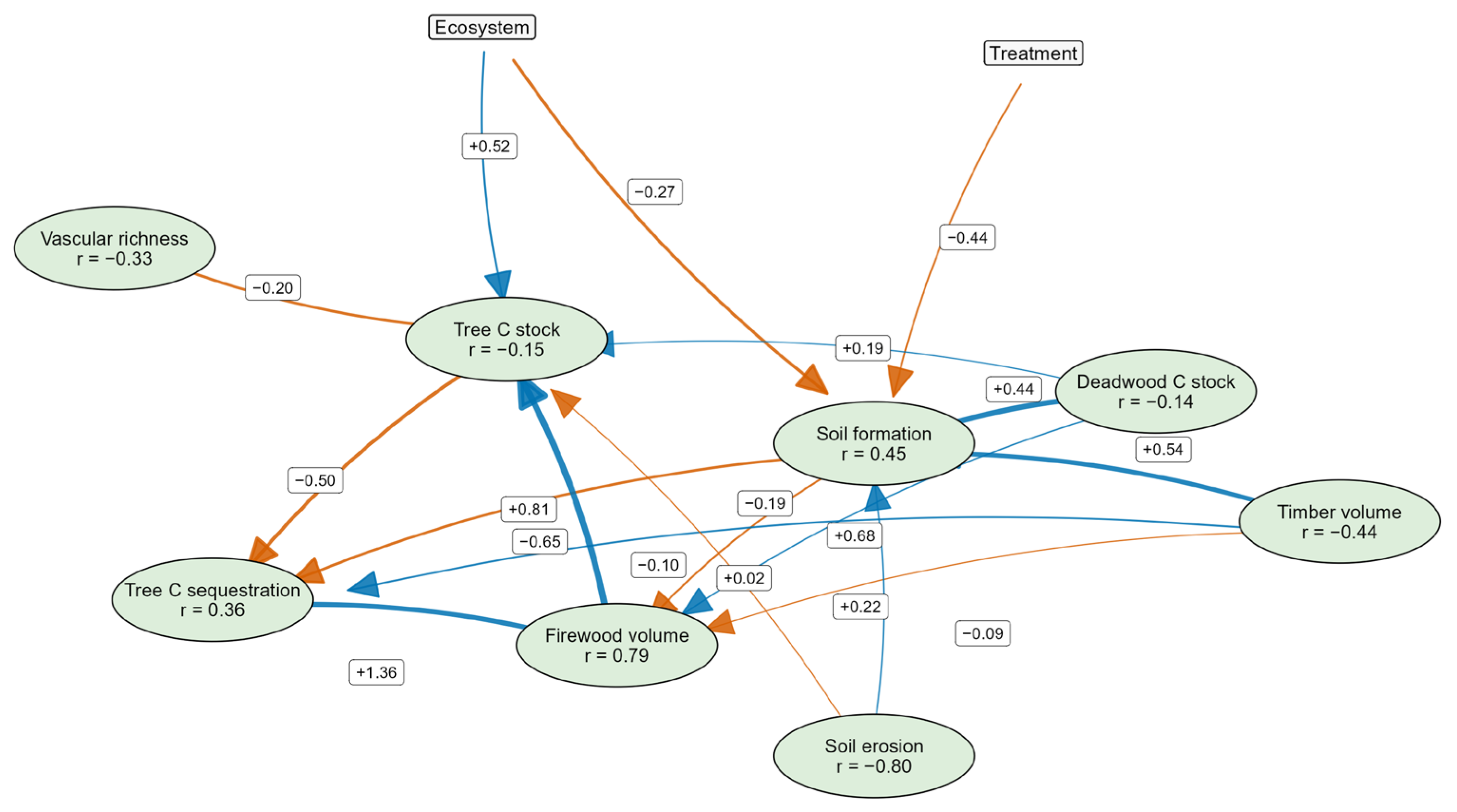
The watershed-scale network was formulated around eight terrestrial ecosystem functions and two exogenous predictors, ecosystem and treatment. The final network retained 17 arcs among these variables (
Figure 1). No previous node-to-node connection was imposed, so the links shown in the network represent relationships retained by the final averaged structure.
Predictive performance was heterogeneous among functions. The highest mean predictive correlations were observed for firewood volume (r = 0.79), soil formation (r = 0.45), and tree carbon sequestration (r = 0.36). Predictive correlations were weaker or negative for deadwood carbon stock (r = −0.14), tree carbon stock (r = −0.15), vascular richness (r = −0.33), timber volume (r = −0.44), and soil erosion (r = −0.80). Thus, at the catchment scale, the network identified a structured set of relationships among functions, but not all functions were predicted with the same reliability.
Ecosystem context was retained as a parent node of tree carbon stock and soil formation. Dry watersheds had 51.94 t C ha−1 higher tree carbon stock than humid watersheds (std. beta = +0.52), but 377.79 m3 ha−1 lower soil formation (std. beta = −0.27). Treatment was also retained as a parent of soil formation: impacted watersheds had 661.87 m3 ha−1 lower soil formation than reference watersheds (std. beta = −0.44). These relationships show that broad ecosystem setting and impact status were part of the retained functional structure at the watershed scale.
The aboveground carbon block was centered on tree carbon stock and tree carbon sequestration, but the two variables did not respond identically. As expected, tree carbon stock increased with firewood volume, with each 1 m3 ha−1 increase in firewood volume associated with 1.33 t C ha−1 higher tree carbon stock (std. beta = +0.81). Tree carbon stock also increased with deadwood carbon stock: each 1 t C ha−1 increase in deadwood carbon stock was associated with 0.50 t C ha−1 higher tree carbon stock (std. beta = +0.19). In contrast, vascular richness was negatively associated with tree carbon stock: each additional vascular plant species was associated with 1.53 t C ha−1 lower tree carbon stock (std. beta = −0.20).
Tree carbon sequestration was most strongly linked to firewood volume. Each 1 m3 ha−1 increase in firewood volume was associated with 0.096 t C ha−1 yr−1 higher tree carbon sequestration (std. beta = +1.36). Tree carbon stock and soil formation showed negative local relationships with tree carbon sequestration: each 1 t C ha−1 increase in tree carbon stock was associated with 0.021 t C ha−1 yr−1 lower sequestration (std. beta = −0.50), and each 1 m3 ha−1 increase in soil formation was associated with 0.002 t C ha−1 yr−1 lower sequestration (std. beta = −0.65).
Timber volume had only a near-zero positive local relationship with tree carbon sequestration (0.062 t C ha−1 yr−1 per 1 m3 ha−1; std. beta = +0.02). Firewood volume was linked to the same wood-soil block: each 1 t C ha−1 increase in deadwood carbon stock was associated with 1.11 m3 ha−1 higher firewood volume (std. beta = +0.68), whereas timber volume and soil formation had negative local relationships with firewood volume (std. beta = −0.09 and −0.19, respectively).
Soil formation occupied a central position in the watershed network. It increased with deadwood carbon stock, timber volume, and soil erosion. Each 1 t C ha−1 increase in deadwood carbon stock was associated with 16.73 m3 ha−1 higher soil formation (std. beta = +0.44), and each 1 m3 ha−1 increase in timber volume was associated with 455.51 m3 ha−1 higher soil formation (std. beta = +0.54). Soil erosion also showed a positive local relationship with soil formation, with each 1 m3 ha−1 increase in soil erosion associated with 0.016 m3 ha−1 higher soil formation (std. beta = +0.22).
3.2. Model 2. Forest-Cluster Ecosystem-Function Network
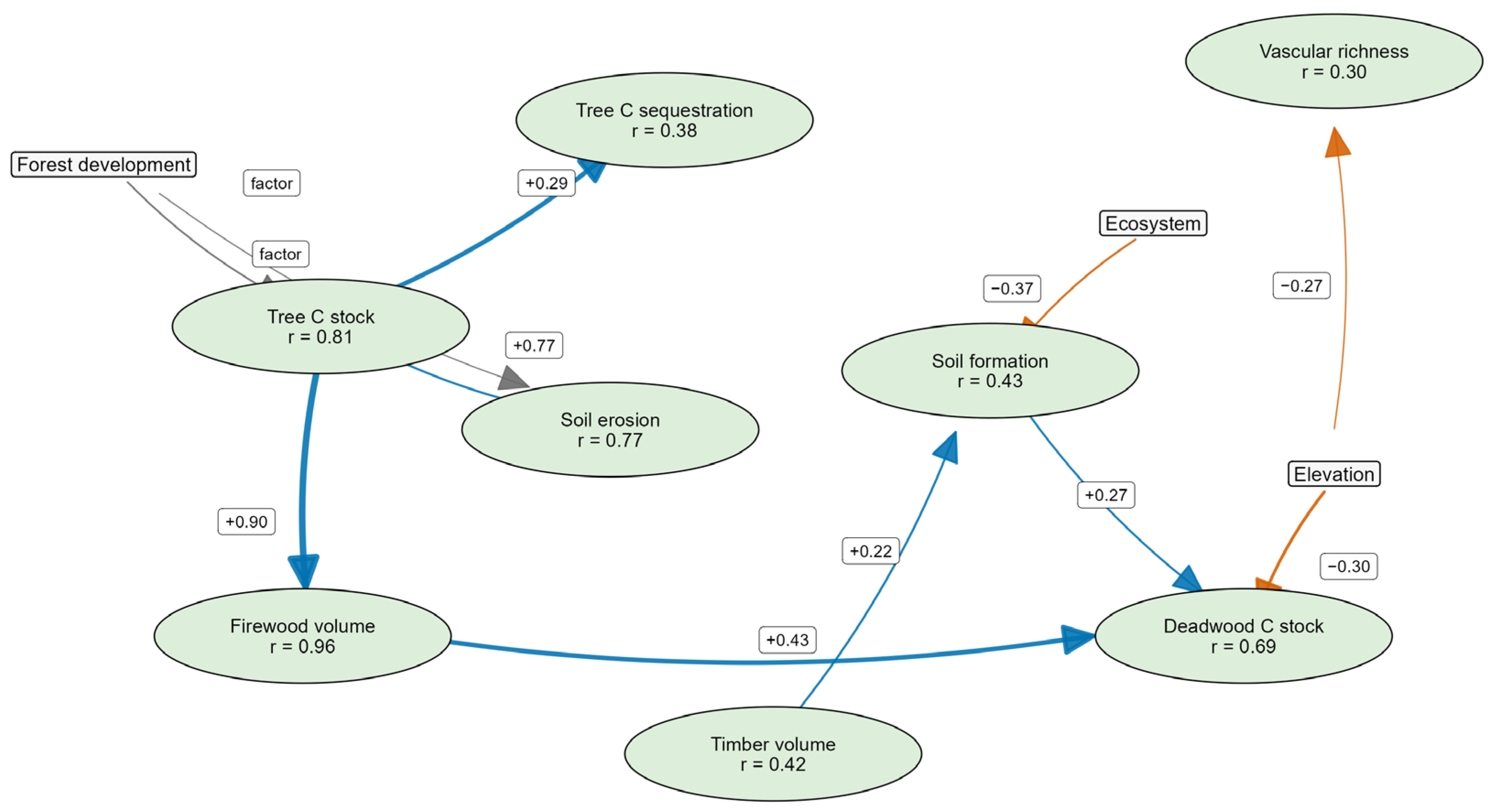
The forest-cluster network represented ecosystem-function relationships among 63 forest clusters (
Figure 2). The selected covariates included ecosystem, elevation, and forest development stage. The final network retained 11 arcs and concentrated the retained structure on the wood–carbon–soil function block.
Compared with the watershed model, predictive performance was stronger and more consistent across forest-cluster functions. Firewood volume had the highest mean predictive correlation (r = 0.96), followed by tree carbon stock (r = 0.81), soil erosion (r = 0.77), and deadwood carbon stock (r = 0.69). Predictive correlations were intermediate for soil formation (r = 0.43), timber volume (r = 0.42), and tree carbon sequestration (r = 0.38), and lower for vascular richness (r = 0.30). The updated cluster-scale model therefore retained strong predictive capacity for the wood and carbon components, while vascular richness was represented by a single environmental link rather than by the central wood–carbon–soil block.
Environmental context was incorporated into the forest-cluster network through ecosystem and elevation. Dry clusters had 843.99 m3 ha−1 lower soil formation than humid clusters (std. beta = −0.37). Elevation was associated with deadwood carbon stock: each 100 m increase in elevation was associated with 3.04 t C ha−1 lower deadwood carbon stock (std. beta = −0.30). Elevation was also associated with vascular richness: each 100 m increase in elevation was associated with 1.15 fewer vascular plant species (std. beta = −0.27).
Forest development stage was retained as a categorical parent of tree carbon stock and soil erosion. Mean tree carbon stock increased from sapling clusters (3.17 t C ha−1) to secondary-growth clusters (127.01 t C ha−1) and adult forest clusters (204.60 t C ha−1), with old-growth clusters showing 170.74 t C ha−1. Soil erosion also varied among development stages, with mean values of 313.46 m3 ha−1 in sapling clusters, 29,889.36 m3 ha−1 in secondary-growth clusters, 27,070.49 m3 ha−1 in adult forest clusters, and 38,146.90 m3 ha−1 in old-growth clusters. These patterns indicate that forest structural condition remained part of the cluster-scale carbon and erosion structure.
The wood–carbon block was the clearest component of the updated cluster network. Each 1 t C ha−1 increase in tree carbon stock was associated with 0.011 t C ha−1 yr−1 higher tree carbon sequestration (std. beta = +0.29), 0.417 m3 ha−1 higher firewood volume (std. beta = +0.90), and 17.83 m3 ha−1 higher soil erosion (std. beta = +1.51). Firewood volume, in turn, was positively associated with deadwood carbon stock: each 1 m3 ha−1 increase in firewood volume was associated with 0.148 t C ha−1 higher deadwood carbon stock (std. beta = +0.43).
Soil formation was connected to both deadwood carbon stock and timber volume. Each 1 m3 ha−1 increase in soil formation was associated with 0.013 t C ha−1 higher deadwood carbon stock (std. beta = +0.27), while each 1 m3 ha−1 increase in timber volume was associated with 20.97 m3 ha−1 higher soil formation (std. beta = +0.22). Together, these relationships show that the updated forest-cluster network is less diffuse than the previous version and is organized mainly around tree carbon stock, firewood volume, deadwood carbon stock, soil formation, timber volume, and soil erosion, with vascular richness entering through elevation.
3.3. Model 3. Plot-Scale Ecosystem-Function Network
The plot-scale network represented ecosystem-function relationships among 175 complete forest plots (
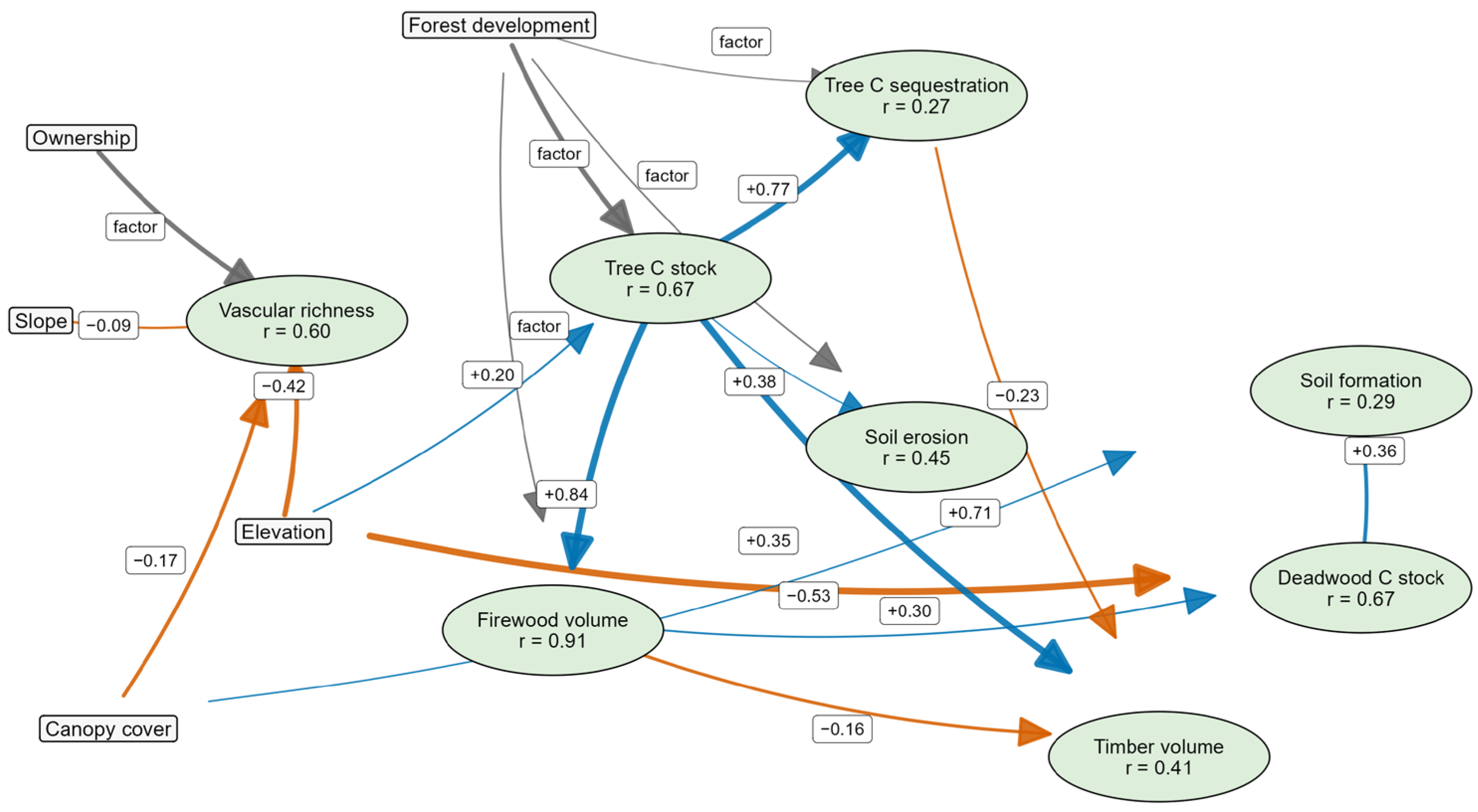
Figure 3). The model included plot-level descriptors as exogenous covariates and retained 19 arcs in the final network. The retained structure allowed environmental and stand descriptors to inform ecosystem functions while keeping the functional relationships among response nodes data-driven.
Predictive performance again varied among functions, but the strongest plot-scale signals were concentrated in the wood and carbon block. Firewood volume had the highest mean predictive correlation (r = 0.91), followed by deadwood carbon stock (r = 0.67), tree carbon stock (r = 0.67), and vascular richness (r = 0.60). Predictive correlations were intermediate for soil erosion (r = 0.45) and timber volume (r = 0.41), and lower for soil formation (r = 0.29) and tree carbon sequestration (r = 0.27). Thus, at the plot scale, the network most clearly captured relationships involving standing carbon, firewood volume, deadwood carbon, vascular richness, and soil erosion.
Plot-level covariates entered the retained network primarily through plant species richness and carbon-related nodes. Richness was associated with ownership, canopy cover, elevation, and slope. Among numeric predictors, richness decreased with canopy cover, elevation, and slope: each 1% increase in canopy cover was associated with 0.064 fewer plant species (std. beta = −0.17), each 100 m increase in elevation was associated with 0.77 fewer species (std. beta = −0.42), and each 1% increase in slope was associated with 0.041 fewer species (std. beta = −0.09). Ownership was retained as a categorical parent of richness. Mean richness was highest in plots under small landowners (11.40 species), followed by national park plots (9.62 species), public lands (7.59 species), and large landowners (2.83 species).
Elevation was also connected to tree carbon stock and deadwood carbon stock. Each 100 m increase in elevation was associated with 7.10 t C ha−1 higher tree carbon stock (std. beta = +0.20) and 5.49 t C ha−1 lower deadwood carbon stock (std. beta = −0.53). Canopy cover was additionally connected to soil formation: each 1% increase in canopy cover was associated with 6.27 m3 ha−1 higher soil formation (std. beta = +0.35).
Forest development stage was retained as a categorical parent of tree carbon stock, tree carbon sequestration, firewood volume, and soil erosion. These relationships indicate that plot context did not enter the model as a diffuse background signal. Instead, it was channeled through a small set of biodiversity, carbon, wood-volume, soil-formation, and erosion responses. Mean tree carbon stock increased from sapling plots (7.88 t C ha−1) to secondary-growth plots (139.08 t C ha−1), adult forest plots (202.77 t C ha−1), and old-growth plots (189.11 t C ha−1). Tree carbon sequestration was highest in secondary-growth plots (3.70 t C ha−1 yr−1), followed by adult forest (2.30 t C ha−1 yr−1), old-growth (2.30 t C ha−1 yr−1), and saplings (0.35 t C ha−1 yr−1) plots. Firewood volume increased from saplings (3.45 m3 ha−1) to secondary growth (58.68 m3 ha−1), adult forest (78.77 m3 ha−1), and old growth (117.94 m3 ha−1). Mean soil erosion was lowest in saplings (23,509.62 m3 ha−1) and highest in old-growth plots (32,743.01 m3 ha−1), with secondary-growth and adult forest plots at 26,022.37 and 31,815.00 m3 ha−1, respectively.
The plot-scale carbon and wood block showed a coherent set of positive relationships. Each 1 t C ha−1 increase in tree carbon stock was associated with 0.016 t C ha−1 yr−1 higher tree carbon sequestration (std. beta = +0.77), 0.064 m3 ha−1 higher timber volume (std. beta = +0.71), and 0.401 m3 ha−1 higher firewood volume (std. beta = +0.84). Firewood volume, in turn, was positively associated with deadwood carbon stock: each 1 m3 ha−1 increase in firewood volume was associated with 0.108 t C ha−1 higher deadwood carbon stock (std. beta = +0.30). Deadwood carbon stock was positively associated with soil formation, with each 1 t C ha−1 increase in deadwood carbon stock associated with 19.05 m3 ha−1 higher soil formation (std. beta = +0.36). Tree carbon stock was also retained as a parent of soil erosion. This relationship was scale-dependent: the coefficient estimated from the log-transformed data used for network fitting was positive (std. beta = +0.38), whereas the local model refitted in original units indicated that each 1 t C ha−1 increase in tree carbon stock was associated with 3.58 m3 ha−1 lower soil erosion. This difference reflects the strongly right-skewed distribution of soil erosion. The original-scale coefficient gives greater influence to large absolute erosion values, whereas the logarithmic transformation reduces their influence and represents relative differences within the fitted network. Not all wood-related links were positive. Firewood volume had a negative local relationship with timber volume: each 1 m3 ha−1 increase in firewood volume was associated with 0.036 m3 ha−1 lower timber volume (std. beta = −0.16). Tree carbon sequestration was also negatively associated with timber volume, with each 1 t C ha−1 yr−1 increase in sequestration associated with 0.415 m3 ha−1 lower timber volume (std. beta = −0.23), despite its weak positive relationship with firewood volume (0.214 m3 ha−1 per 1 t C ha−1 yr−1; std. beta = +0.03). These mixed signs show that timber volume was not simply interchangeable with firewood volume or sequestration at the plot scale.
3.4. Cross-Scale Synthesis
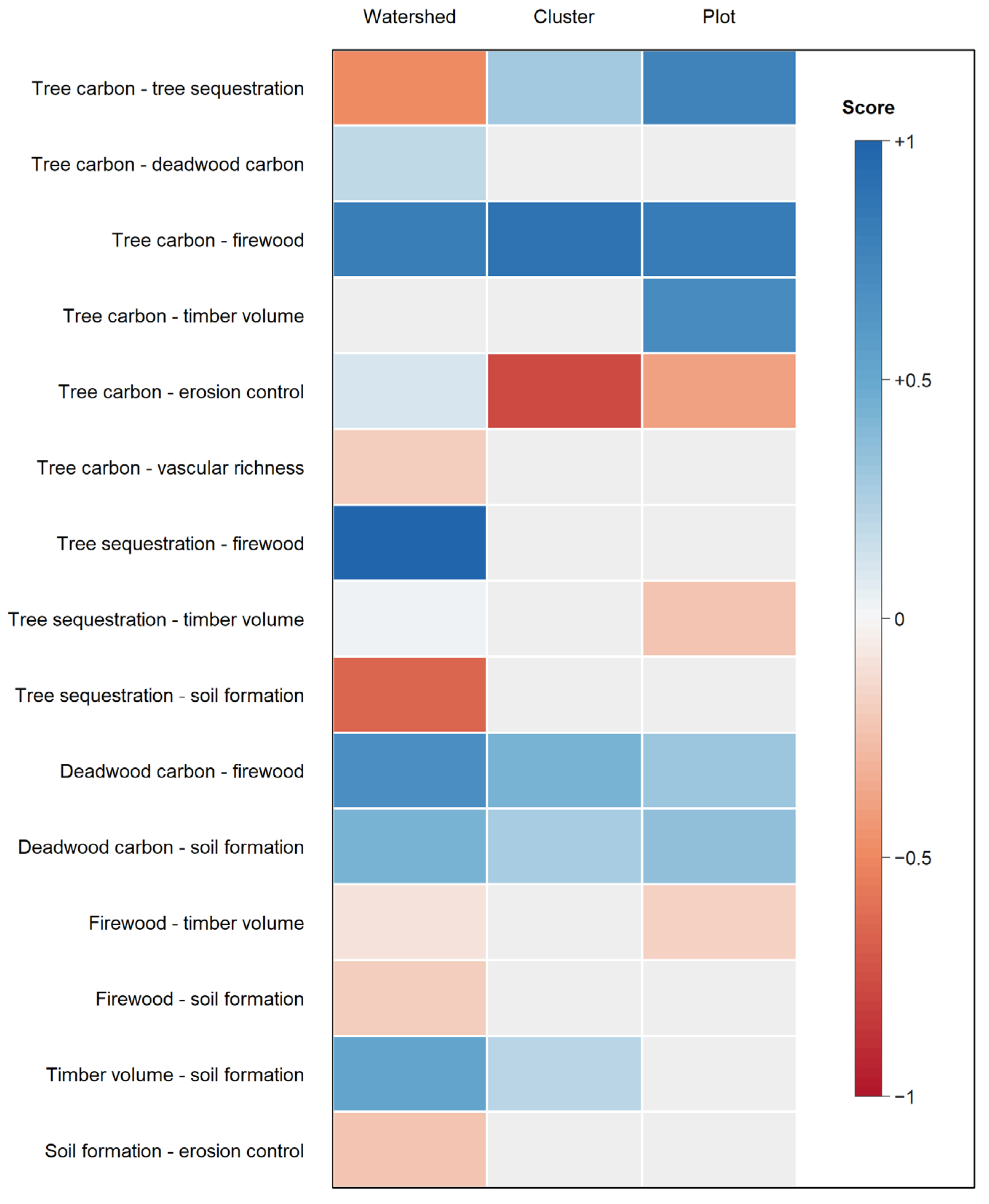
Overall, the final models show that ecosystem multifunctionality in the study system was structured by scale (
Figure 4). Across models, firewood volume and tree carbon stock repeatedly emerged as highly connected and comparatively well-predicted functions. Deadwood carbon stock and soil formation were also consistently linked, especially at the cluster and plot scales, where their positive relationship was retained in the final networks. Vascular richness behaved differently from the carbon and wood functions: it was more directly associated with environmental or contextual covariates than with the central carbon-production block. This cross-scale pattern indicates that the network did not collapse into a single multifunctionality gradient. Instead, it revealed partially connected subsystems, with carbon and wood production forming the most recurrent functional module and vascular richness responding more strongly to site context.
3.5. Conditional Trade-Offs and Synergies Along the Tree Carbon Stock Gradient
The conditional response profiles showed that the association between tree carbon stock and the other ecosystem functions was not uniform across scales or conditioning factors. Across the three models, firewood volume, deadwood carbon stock, and tree carbon sequestration most often increased with higher tree carbon stock. These responses represent conditional synergies with tree carbon stock. Vascular richness was mostly flat or decreased along the same gradient, while erosion control changed direction among scales and forest development stages.
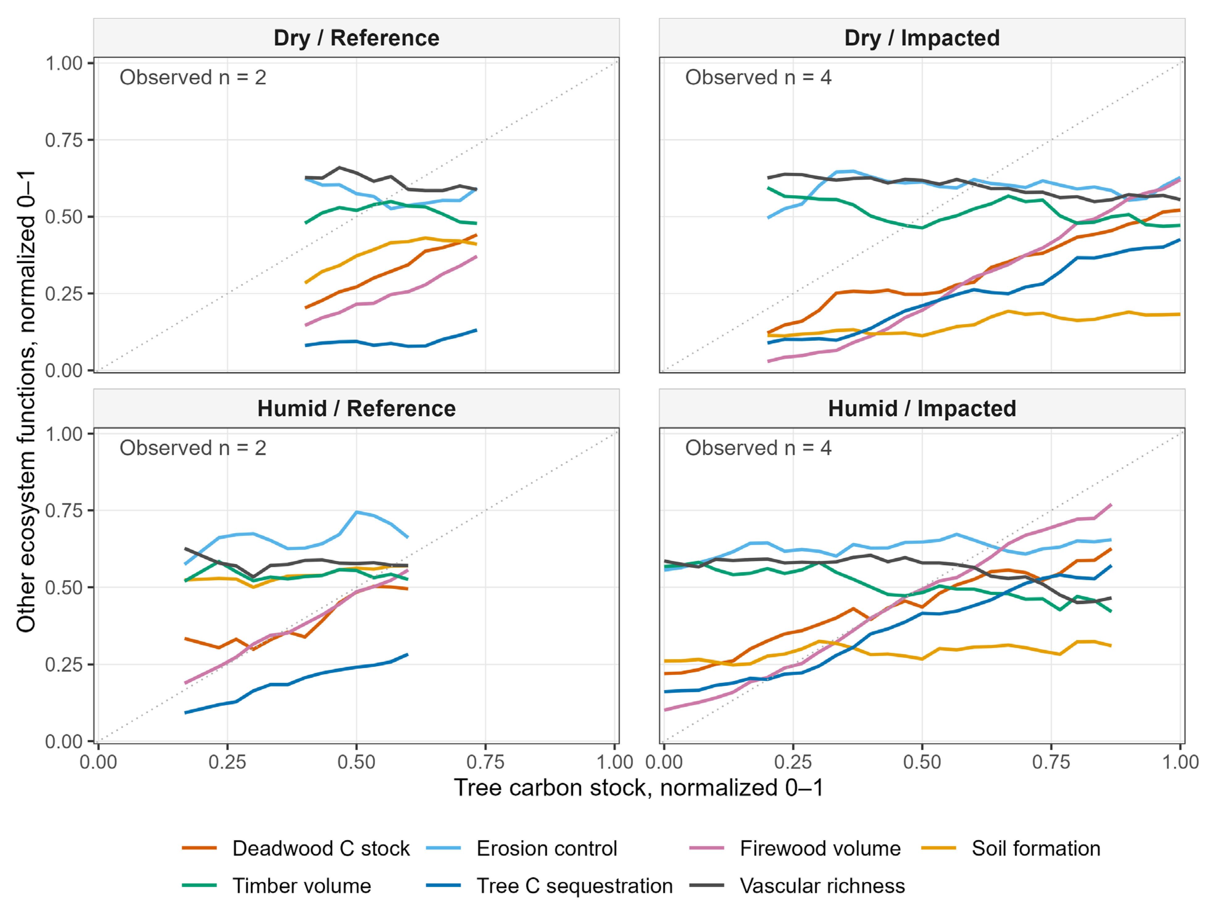
At the watershed scale, the strongest positive responses to higher tree carbon stock were firewood volume, deadwood carbon stock, and tree carbon sequestration (
Figure 5). Firewood volume increased in all four ecosystem-treatment combinations, with the largest changes in humid-impacted watersheds (0.10 to 0.77 on the normalized scale) and dry-impacted watersheds (0.03 to 0.62). Deadwood carbon stock also increased in all four combinations, with normalized changes of 0.16 to 0.41. Tree carbon sequestration increased most clearly in disturbed catchments, especially humid-impacted watersheds (0.16 to 0.57) and dry-impacted watersheds (0.09 to 0.43). Vascular richness decreased in all four combinations. Timber volume also decreased in the two impacted combinations and remained almost flat in reference watersheds. Erosion control increased in humid reference, humid impacted, and dry-impacted watersheds, but was slightly lower along the carbon gradient in dry reference watersheds. Because Model 1 had low support within each ecosystem-treatment combination, these profiles are shown without confidence intervals.
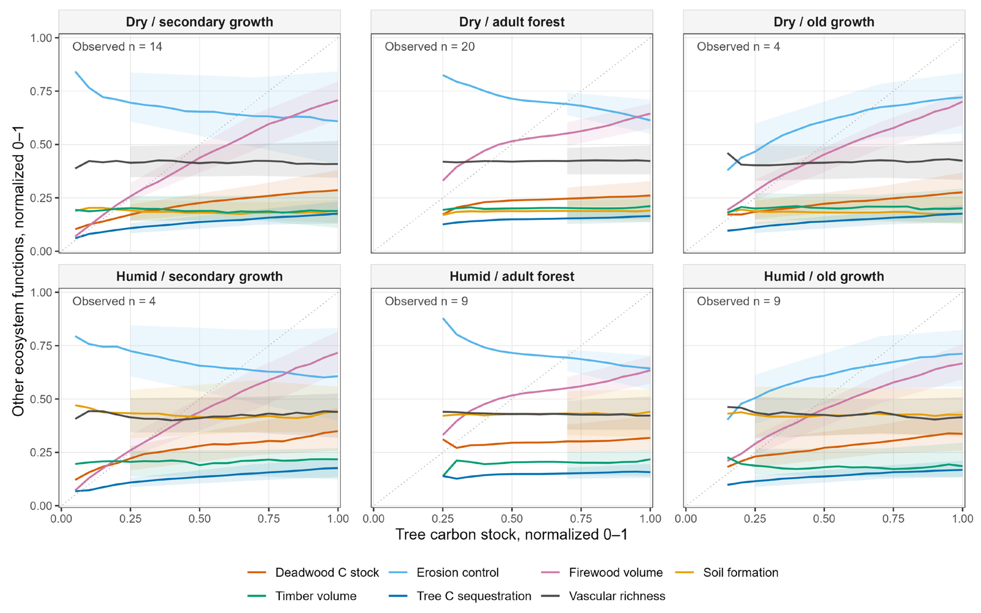
At the forest-cluster scale, firewood volume was the most consistent positive response across all ecosystem and development-stage combinations (
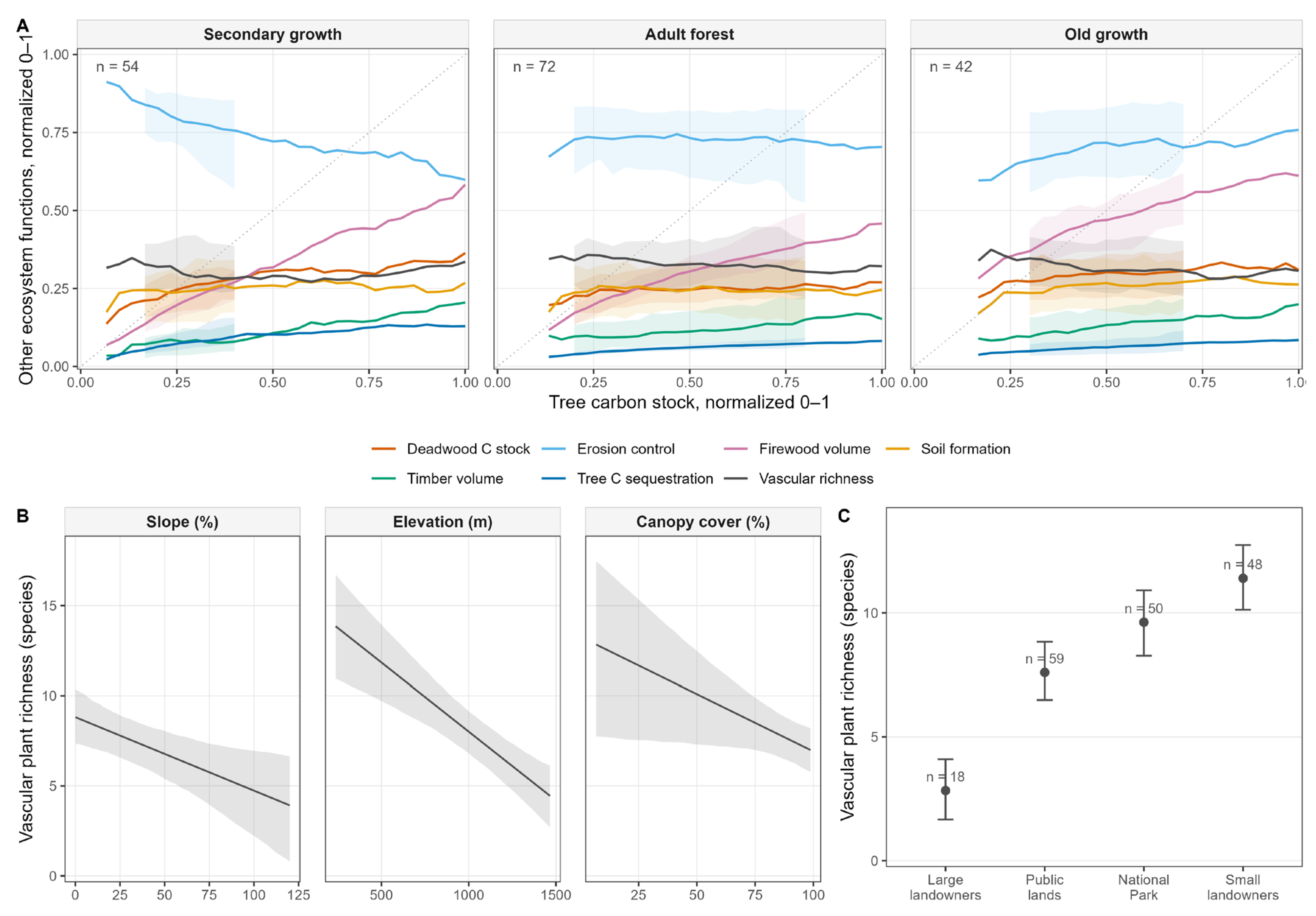
Figure 6). The increase was strongest in secondary-growth clusters, both dry (0.07 to 0.71) and humid (0.07 to 0.72), and remained positive in adult forest and old-growth clusters. Deadwood carbon stock also increased in most combinations, with larger changes in secondary-growth clusters and old-growth clusters than in adult forest. Tree carbon sequestration generally increased with tree carbon stock, although the change was small in humid adult forest. Timber volume and soil formation were mostly flat, with small positive or negative changes depending on the panel. Vascular richness was mainly flat, except for small decreases in old-growth clusters and a small increase in humid secondary-growth clusters. Erosion control showed the strongest scale- and stage-dependent pattern: it decreased in secondary-growth and adult forest clusters but increased in old-growth clusters in both dry and humid ecosystems.
At the plot scale, the development-stage profiles again showed positive responses of firewood volume, deadwood carbon stock, tree carbon sequestration, timber volume, and soil formation along the tree carbon stock gradient (
Figure 7A). The largest increase was observed for firewood volume, especially in secondary-growth plots (0.07 to 0.58), adult forest plots (0.12 to 0.46), and old-growth plots (0.28 to 0.61). Deadwood carbon stock and timber volume also increased in the three displayed development stages. Vascular richness was nearly flat in secondary-growth and adult forest plots and decreased slightly in old-growth plots (0.34 to 0.31). Erosion control decreased strongly in secondary-growth plots (0.91 to 0.60) but increased slightly in adult forest and more clearly in old-growth plots.
The plot-level vascular-richness analysis in original units showed negative responses to the three numeric parents retained in the local model (
Figure 7B). Expected vascular richness decreased from 12.84 to 7.00 species along the observed canopy-cover range, from 13.85 to 4.45 species along the observed elevation range, and from 8.82 to 3.92 species along the observed slope range. Ownership also separated vascular richness among plots (
Figure 7C). Mean vascular richness was highest under small landowners (11.40 species; 95% bootstrap interval 10.13–12.74), followed by national park plots (9.62; 8.27–10.91), public lands (7.59; 6.49–8.83), and large landowners (2.83; 1.67–4.10).
4. Discussion
This study asked how environmental conditions, disturbance, and spatial scale drive conditional dependencies among ecosystem functions in Patagonian headwater catchments. These dependencies were not organized as a single fixed gradient of multifunctionality. Instead, the three final Bayesian network models showed a scale-dependent structure in which some functions formed recurrent positive blocks, while others were linked to environmental or contextual drivers [
8,
10,
11].
Overall, the results suggest that some associations among ecosystem functions should not be interpreted as direct function–function relationships, because they may arise from shared responses to environmental or contextual drivers [
15,
16,
18]. They also support the findings of previously reported studies that suggest tree carbon stock and biomass-related functions share structural links, while sequestration is not fully interchangeable with accumulated stocks. The hypothesis about disturbance and biodiversity was only partly supported: impact status and forest development were related to carbon, soil, and erosion responses, but vascular richness was not simply reduced or increased by a single driver [
19,
20,
21]. Instead, it depended on local and contextual conditions such as elevation, canopy cover, slope, and ownership. The strongest general result is therefore not that one function controls the others, but that the functional structure of these catchments changes with drivers and scale [
22,
23].
4.1. Trade-Offs, Synergies and Shared Drivers
A central result of the analysis is that trade-offs and synergies among ecosystem functions were not fixed pairwise, one-to-one relationships. They depended on the drivers included in the networks, the conditioning factors used in the profiles, and the scale at which the functions were observed. This distinction matters because two functions can be associated because they are conditionally linked within the network, but they can also be associated because both respond to a common driver such as climate, forest development, elevation, canopy cover, or disturbance history [
15,
16]. Pairwise correlations alone cannot separate these alternatives and may therefore misidentify driver-mediated complex relationships as direct trade-offs or synergies [
17,
18].
The conditional profiles along the tree carbon stock gradient provided a network-based way to read these relationships. Following a probabilistic interpretation of trade-offs and synergies [
28], a positive conditional response of one function when tree carbon stock was higher was treated as a synergy, while a negative response was treated as a trade-off. This approach differs from a simple correlation analysis because the response is evaluated within the fitted conditional structure and, for Models 2 and 3, under explicit conditioning factors and bootstrap uncertainty. Similar forest studies have also shown that interactions and joint production among timber, carbon, water, and biodiversity-related outputs can depend on stand age, silvicultural treatment, site quality, weather, ownership, and other biophysical or management drivers [
37,
38].
Across scales, the most consistent synergy was between tree carbon stock and firewood volume (
Figure 4). Deadwood carbon stock also tended to increase with tree carbon stock, especially at the cluster and plot scales, where firewood volume connected positively to deadwood carbon stock and deadwood carbon stock connected to soil formation (
Figure 2 and
Figure 3). This forest deadwood signal is consistent with recent evidence from Patagonian headwater streams, where high instream wood abundance reflected both local channel retention and the availability of deadwood and carbon stocks in the surrounding forest matrix [
39]. Tree carbon sequestration often increased with tree carbon stock, but this relationship was less uniform. This is ecologically plausible because stock and sequestration are related but not equivalent: stock is an accumulated state, while sequestration is a rate that can peak under different stand-development conditions. Similar patterns have been reported in forest studies that link tree biomass, carbon storage, timber production, soil carbon, water yield, and biodiversity-related outputs and show that these relationships can vary with forest attributes, environmental conditions, and management context [
9,
11,
37,
38]. This interpretation is also consistent with recent Chilean forest evidence showing that soil carbon responds to multiple climatic, topographic, stand, and human-impact drivers, and that tree and soil pools jointly dominate forest carbon stocks but shift in relative importance with forest condition [
40,
41].
The clearest trade-off signal involved vascular richness, but this result was also driver-dependent. Vascular richness was mostly flat or negative along the tree carbon stock gradient (
Figure 5,
Figure 6 and
Figure 7), and the plot-level raw-unit analysis showed lower expected richness with higher canopy cover, elevation, and slope (
Figure 7B). This pattern should not be read as a universal direct trade-off between vascular richness and carbon storage. Ownership classes also differed strongly in vascular richness, and the network did not support a simple biodiversity-carbon mechanism. Instead, the result is better read as a conditional divergence between carbon-related functions and vascular richness under the observed environmental and land-tenure structure [
19,
20,
21]. For example, vascular richness decreased by 1.15 species for each 100 m increase in elevation. This decline may partly reflect the lower temperatures and more restrictive growing conditions at higher elevations, which may limit the persistence of vascular plant species. Another example concerns ownership type, as vascular richness differed among ownership categories. However, because management intensity and specific management practices were not measured independently, the mechanism underlying this association remains uncertain and cannot be attributed directly to either management practices or ownership itself.
Erosion control showed the strongest context dependence. It did not behave as a stable synergy or trade-off with tree carbon stock. At the cluster scale, erosion control decreased along the carbon gradient in secondary-growth and adult forest clusters but increased in old-growth clusters (
Figure 6). At the plot scale, it decreased strongly in secondary-growth plots but increased slightly or clearly in adult and old-growth plots (
Figure 7A). This pattern suggests that the relationship between carbon storage and erosion regulation depends on forest development stage [
41] and possibly on local geomorphic conditions. It also shows why a single overall multifunctionality score would hide important contrasts among functions [
8]. The conditional erosion profiles may also reflect differences in forest recovery and structural complexity. In secondary-growth clusters, carbon accumulation may be concentrated in the developing tree canopy, while understory cover, litter accumulation, coarse woody material, root structure, and other protective attributes have not yet recovered to old-growth conditions. In contrast, the increase in erosion control with tree carbon stock in old-growth clusters is consistent with structurally complex forests, where canopy interception, litter, roots, understory vegetation, and deadwood can reduce raindrop impact and surface runoff. These mechanisms are proposed as plausible interpretations rather than demonstrated causal pathways.
Taken together, the results point to a carbon and wood production block, but not to a single multifunctionality axis. Tree carbon stock, firewood volume, tree carbon sequestration, deadwood carbon stock, and some soil responses were linked through forest development and site context. Vascular richness followed a more local and context-dependent path, so its response to disturbance or management must be evaluated directly rather than inferred from carbon or wood variables.
4.2. Scale Dependence and Implications for Monitoring
The three networks also show that the scale of observation changes both the strength and the directional relationships among functions. This agrees with previous work showing that ecosystem-service or ecosystem-function relationships can change in direction, magnitude, and significance across spatial scales [
22,
23]. In this study, the watershed model summarized the full catchment mosaic, including differences between dry and humid ecosystems and between reference and impacted catchments. This scale is useful for catchment-level synthesis, but it also had the smallest sample size and the weakest predictive performance for several nodes (ecosystem functions). Thus, the watershed network should be read as a constrained probabilistic synthesis of broad patterns, not as a general structure-learning model.
The forest-cluster model provided the clearest balance between ecological resolution and predictive stability. It retained strong predictive performance for firewood volume, tree carbon stock, soil erosion, and deadwood carbon stock, while keeping vascular richness in a more peripheral and environmentally mediated position (
Figure 2). This suggests that the cluster scale is well suited for detecting the main forest-function module. At this level, aggregation reduced some plot-level noise while still preserving meaningful variation in forest development, elevation, and ecosystem context. Timber volume showed only intermediate predictive performance despite its position in the cluster network. Unlike tree carbon stock and firewood volume, timber volume represents a selective component of forest structure because it depends on the presence of stems meeting merchantable criteria. Its variation may therefore depend on stand characteristics not fully represented by the retained parent nodes.
The plot-scale model added a complementary view. It was not intended to replace the cluster model, because plots are nested within clusters and local observations are not fully independent at the landscape scale. Instead, it worked as a sensitivity analysis showing which relationships sharpen or change when local covariates are retained. The plot model confirmed the repeated positive structure among tree carbon stock, firewood volume, timber volume, tree carbon sequestration, and deadwood carbon stock. It also made the drivers of vascular richness more explicit. This supports the broader conclusion that some relationships are stable enough to appear across scales, while others are only visible when the appropriate spatial unit and covariates are used [
17,
22].
For monitoring, this means that no single scale is enough to answer the research question. Catchments are appropriate for integrating the full mosaic and comparing broad ecosystem and treatment contexts, but they are too coarse and too few to reveal all local mechanisms. Forest-cluster scales appear to be the most informative level for monitoring the recurrent wood–carbon–soil module in this inventory because they retained strong predictive performance without losing stand-level ecological meaning. Plots are most useful for detecting local driver effects, especially for vascular richness [
2,
21,
22]. In practical terms, forest clusters comprise nearby sampling units located within approximately 100 m of one another and represent a stand context with broadly similar characteristics. Individual plots constitute the basic sampling unit and capture finer-scale differences within that context, including variation in forest development stage, aspect, canopy cover, and other local conditions. Thus, cluster-level monitoring can characterize the predominant functional structure of a forest stand, whereas plot-level observations complement it by identifying local heterogeneity that may be obscured through aggregation.
4.3. Implications for Catchment Management
Following the previous monitoring discussion, the main implication for monitoring and management is that carbon-centered indicators are informative but incomplete. Tree carbon stock and firewood volume were central and well-predicted in the forest models, so they can be useful indicators of a broader wood–carbon functional module. Nevertheless, they do not replace direct monitoring of vascular richness or soil-related functions. Vascular richness responded to a different set of local conditions, and erosion control changed direction depending on scale and forest development stage. Management actions that increase carbon storage or woody biomass may therefore generate synergies with some functions, but they should not be assumed to improve all functions simultaneously [
8,
11,
42].
The selection of monitoring units and indicators should therefore follow the management objective. Carbon storage and wood-related objectives can be evaluated primarily at the forest-cluster scale by integrating tree carbon stock, timber, firewood, and deadwood indicators within broadly comparable forest stands. Objectives focused on vascular diversity or responses to local forest conditions require plot-level observations capable of capturing variation in forest development stage, aspect, canopy cover, and other local attributes. Soil-regulation objectives may require information from both scales because erosion responses varied with forest development stage and local conditions. Catchment-scale information is most appropriate when the objective is to place these stand- and plot-level responses within their broader environmental and disturbance context.
The results also refine the interpretation of multifunctionality in southwestern Patagonia. Spatial work in the region has shown broad synergies and multifunctionality hotspots across forest landscapes [
14]. The present study complements that view by showing how relationships look when they are evaluated as conditional dependencies from nested field measurements. The two perspectives are not contradictory. Spatial multifunctionality maps identify where high functional values co-occur across the landscape, while the Bayesian network approach asks how functions and drivers are conditionally related within the observed system. Together, they suggest that Patagonian forests can contain strong multifunctional patterns, but that the mechanisms behind those patterns may differ among functions, drivers, and scales.
These findings are especially relevant for headwater catchments because management units often integrate vegetation, soils, and disturbance histories within relatively bounded environmental settings [
43]. Mountain catchments tend to be more internally constrained than large continental basins or river systems draining to the sea, which may integrate multiple climates, land uses, and hydro-ecological drivers. In those larger systems, average ecosystem-function values can be difficult to interpret as management targets. Even within these smaller mountain systems, however, a catchment-level indicator may be useful for regional planning but can hide plot- or stand-level mechanisms. Conversely, a plot-level relationship may not scale directly to the catchment because plots are embedded in broader mosaics and ecosystem-service relationships can change across spatial scales [
22]. The nested design used here helps connect these levels without forcing all functions into a single scale of analysis.
This management interpretation, however, depends on management or study objectives. If the goal is to evaluate how environmental drivers, disturbance, and scale structure conditional dependencies among functions, then management should avoid treating trade-offs and synergies as universal pairwise labels. A carbon-biodiversity contrast detected under one set of local conditions may not have the same meaning at the catchment scale. Likewise, a carbon–wood synergy that is robust inside forest stands does not guarantee a positive response of soil regulation or vascular richness. Susaeta et al. [
38] reached a related management conclusion from a production-efficiency perspective in longleaf pine forests: joint production of timber, carbon sequestration, biodiversity, and water yield can respond differently to weather, ownership, disturbance, and silvicultural treatment. The practical value of the Bayesian network approach is that it helps identify where relationships are retained among functions, where they are mediated by drivers, and where uncertainty or scale prevents a strong conclusion. This is consistent with the broader use of Bayesian networks as transparent tools for combining empirical information, ecological restrictions, and uncertainty, while keeping model interpretation explicit [
27,
29].
4.4. Limitations: Small Catchment Sample, Observational Inference and Nested Data
Several limitations should guide interpretation of our approach and findings. First, the watershed model used only twelve catchments. It is therefore useful as a constrained synthesis of the sampled catchments, but not as a freely learned or broadly generalizable network. The low support within some ecosystem-treatment combinations also explains why conditional profiles for Model 1 were shown without confidence intervals (
Figure 5).
Second, all models are observational. The networks describe conditional dependencies under the variables and restrictions included in the analysis, but they do not prove causality. This is a general caution for Bayesian network interpretation, especially when latent or unmeasured drivers may be present [
29]. In this study, unmeasured variation in disturbance history, stand age, management intensity, soil properties, microclimate, herbivory, or past land use could partly mediate some of the observed dependencies. Therefore, the absence of a direct arc or the presence of a conditional association should not be interpreted as definitive evidence that a mechanism is absent or uniquely identified. The restrictions used here reduce ecologically implausible directions and prevent response nodes from explaining exogenous predictors, but they do not remove all possible confounding.
Finally, the three scales differ in sample size, aggregation rules, and ecological meaning. The watershed model includes the broader catchment mosaic, whereas the forest-cluster and plot models are restricted to forest stands. Plots are nested within clusters and clusters within catchments, so observations should not be treated as fully independent across scales. This difference is intentional, but it means that scale comparisons should be read as complementary views rather than as identical models fitted to the same sampling universe.