ALS Pulse Density Effects on Tree Height Accuracy and the Quality of Elevation and Canopy Rasters

Abstract

This study investigated the influence of airborne laser scanning (ALS) pulse density on the accuracy of total tree height estimates and the quality of raster products commonly used in individual tree detection (ITD) workflows. Using a high-density (36 pulses per square meter (PPM)) ALS dataset, we generated lower-density subsets and compared derived outputs using a standardized processing pipeline. Tree height estimates were validated against field measurements, and elevation products—digital elevation models (DEMs), digital surface models (DSMs), and canopy height models (CHMs)—were assessed across pulse densities. DSM and CHM quality improved with increasing density, showing reduced bias and tighter variation. In contrast, DEM accuracy remained relatively stable across densities, indicating lower-density ALS may suffice for ground modeling in forested environments. The results also revealed a strong positive relationship between pulse density and total tree height accuracy. Higher-density datasets consistently produced more accurate and less biased tree height estimates, while sparser datasets exhibited systematic underestimation due to missed canopy peaks. These findings emphasize the importance of aligning ALS pulse density with project objectives. While low-density data may be adequate for terrain modeling, higher-density acquisitions are critical for reliable canopy representation and accurate ITD outputs. This study provides operational guidance for forestry practitioners and highlights the value of investing in higher-resolution ALS data for modern forest inventories.

1. Introduction

Accurate and cost-effective forest inventory is foundational to sustainable forest management, timber valuation, long-term planning, and biomass quantifications to be used in carbon projects. For decades, traditional field-based inventory methods—typically involving systematic plot sampling—have been the industry standard [1,2]. While effective in many respects, these approaches are labor-intensive, costly, and often logistically complex at large scales [3,4]. Consequently, many industrial forest landowners conduct inventories on only a subset of their ownership each year. In addition to high operational costs, traditional sampling methods are vulnerable to design and sampling error [5,6,7], with results highly dependent on plot placement, measurement protocols, and cruiser accuracy. These limitations have driven the forestry sector to explore more efficient, scalable, and objective alternatives.

In the last several decades, advancements in remote sensing have revolutionized forest inventory workflows, with Light Detection and Ranging (LiDAR) emerging as a particularly promising tool [8]. LiDAR technology, which captures high-resolution three-dimensional information about forest structure, has been applied across multiple collection platforms including terrestrial laser scanning (TLS), drone-mounted systems, helicopters, and satellites [9]. ALS is an active remote sensing technology that uses a laser ranging system mounted on an aircraft, together with a scanning mechanism, differential global positioning system (DGPS), and an inertial measurement unit (IMU), to measure the three-dimensional structure of the Earth’s surface by recording the time-of-flight or phase difference of emitted and returned laser pulses [10]. These measurements are combined with precise position and orientation information to produce dense, georeferenced point clouds, which can be processed to generate digital terrain models (DTMs), DSMs, and a wide range of forest structural metrics [10]. Due to its ability to accurately characterize tree crowns and forest canopy structure, ALS has become the preferred remote sensing technology for large-scale forest inventory and assessment applications, including the estimation of forest carbon stocks [11], offering an effective balance of measurement accuracy, spatial coverage, and cost efficiency [12,13,14].

ALS-informed inventory methods have introduced new possibilities for forest data collection [15]. Unlike traditional plot-based methods, ALS can provide temporally consistent wall-to-wall coverage of entire ownerships, significantly reducing the need for extensive field campaigns. While many ALS-based inventory approaches still require some field data for model calibration and validation, the overall demand for fieldwork can be greatly reduced. The most commonly used ALS-based inventory techniques include area-based methods and ITD [16]. Area-based methods typically rely on relationships between ALS point clouds and field data to train statistical or machine learning models that predict forest attributes such as volume, basal area (BA), or tree density at a specified spatial resolution [17,18]. In contrast, ITD methods aim to directly identify and attribute individual trees. This approach has the potential to deliver detailed, near-census-level data across broad spatial extents. ITD inventories are especially valuable when tree-level information—such as species, size, and spatial distribution—is critical.

Standard LiDAR-based methodologies for detecting individual trees include raster-based (most often informed by rasters containing ground and vegetation elevation data), cloud-based (direct from an ALS point cloud), and hybrid approaches (informed by both a CHM and an ALS point cloud) [19,20]. The performance of raster-based segmentations, which are very common in practice and widely available in open source software packages [21,22,23], in coniferous forests is well documented and often very accurate for dominant and codominant stems, i.e., the stems that contribute a large majority of the volume, basal area, and biomass [19,24]. CHMs are the most commonly used input for raster-based ITD segmentation processes. A CHM represents canopy height in raster form and is derived by subtracting a DEM or DTM from a DSM. Consequently, the reliability of raster-based ITD segmentation is highly dependent on the accuracy of the input datasets used to generate the CHM.

Several studies using sparser ALS datasets have demonstrated how reductions in LiDAR data density typically have minimal impact on the quality of resulting DEMs [25,26]. This suggests that DEM generation is relatively robust to lower point densities and is likely suitable for many use cases extending beyond forest inventory and carbon quantification. On the other hand, some studies [26] suggest the use of high-density LiDAR when conducting micro-scale analyses or processing to fine spatial resolutions. Silva et al. (2017) [27] recommended using DTMs derived from high-density LiDAR for change detection and monitoring in areas with steep terrain, where small elevation errors can propagate significantly.

DSMs—and consequently CHMs—are much more sensitive to point density. When creating vegetation surfaces from LiDAR point clouds, Silva et al. (2013) [28] demonstrated that both DSMs and CHMs benefit substantially from higher-density data, even though the “high” density in that study was only 4.5 points per square meter, well below the capabilities of modern sensors. Subsequent research has confirmed that lower-density datasets can still yield reliable DSMs and CHMs for broad-scale analyses, such as area-based biomass estimation [27]. However, applications requiring detailed, object-level delineation—such as ITD—benefit from higher-density inputs. Sparks et al. (2022) [19], for example, showed that increasing pulse density from 8 PPM to 22 PPM in raster-based segmentations significantly improved detection rates. In short, while moderate point densities may suffice for many mapping and modeling purposes, higher densities consistently seem to enhance DSM and CHM quality, improving a variety of applications including ITD and digital Measurement, Reporting, and Verification (MRV) with the intent of enhancing carbon market transparency.

In addition to tree detection, attribution—calculating and assigning individual tree metrics—is equally important. Total height is a fundamental structural attribute that strongly correlates with other important metrics like volume, biomass, and diameter at breast height (DBH), making it a vital predictor in forest modeling and therefore essential to estimate accurately [16,29,30]. ALS is particularly effective for capturing vertical forest structure and, when properly processed, can provide highly accurate height information—often surpassing field measurements [31]. This is especially important to consider in the context of carbon stock quantifications when using industry standard and registry-approved biomass equations, such as those produced by Woodall et al. 2011, that utilize tree height as an input [11,32]. However, not all ALS data are equal; and some datasets may not suffice for the intended use case. For example, sparse ALS datasets can underestimate tree height by missing treetops or failing to accurately detect the ground beneath dense canopy cover [33,34,35,36]. Numerous studies have shown that increasing pulse density enhances ITD and attribution accuracy [19,33,34], yet many of these studies relied on relatively sparse datasets—comparable to or even less dense than those publicly available today. In North America, for instance, most public ALS data are collected at roughly 8 pulses per square meter [37], a level sufficient for coarse surface analyses but often inadequate for precise vegetation characterization [38]. With modern ALS sensors now capable of acquiring much higher pulse densities at relatively lower costs [19,33,39], it is increasingly important to evaluate whether these advancements further enhance ITD input rasters and height estimation accuracy at densities exceeding those examined in previous studies.

When conducting studies of this nature, it is important to recognize potential sources of noise in comparative analyses, including significant time gaps between ALS and field data collection, as well as variations in ALS flight plans. Precisely replicating flight paths, altitudes, and overlap conditions is inherently difficult, potentially introducing discrepancies that affect data comparability [40]. Minimizing the effects of these confounding factors via a highly controlled environment with temporally and spatially consistent datasets is ideal when trying to isolate the true effects of pulse density on tree height estimation and the integrity of generated ITD input rasters.

The objective of this study was two-fold: (1) to leverage a highly controlled environment to document the impact of pulse density on the integrity of surface rasters commonly used as inputs for raster-based ITD workflows (DEM, DSM, CHM), and (2) to evaluate how tree height estimation accuracy changes across a wide range of pulse densities in a complex mixed-species forest. By testing ALS datasets of various densities, we sought to determine whether modern high-density ALS scans offer meaningful improvements over more conventional, lower-density datasets. Ultimately, the findings of this research are intended to support forestry professionals in making informed decisions about the adoption and deployment of ALS technology for forest inventory purposes.

2. Materials and Methods

2.1. Study Area

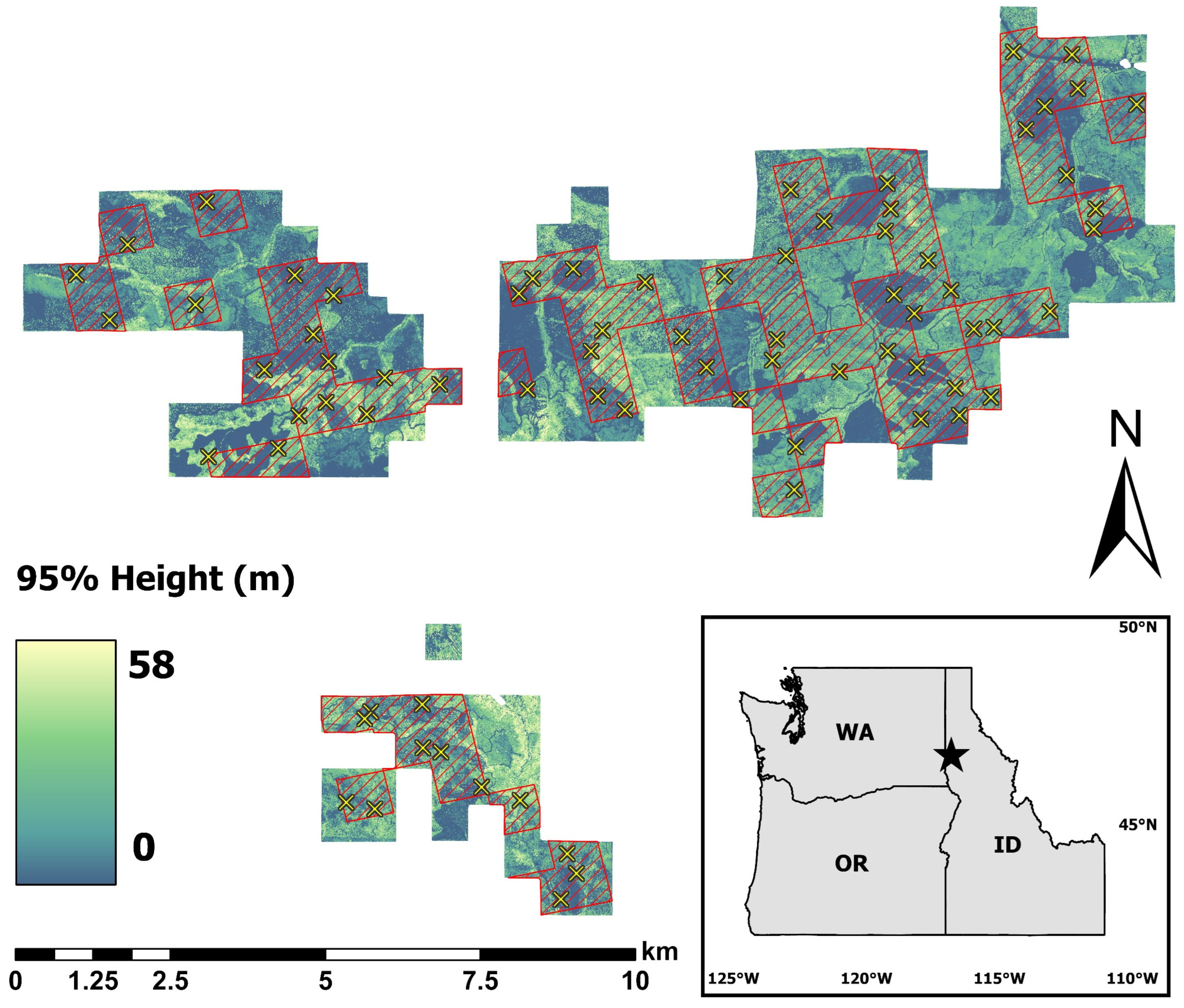
This study was conducted approximately 20 km northeast of Moscow, Idaho, USA, on the University of Idaho experimental forest (UIEF) located in the Palouse Range (Figure 1). The UIEF is a temperate mixed conifer forest composed of stands with various species compositions, ages, and structures that range in elevation from approximately 850 to 1250 m above sea level. Common tree species observed in the study area include Pseudotsuga menziesii (Mirb.) Franco var. glauca (Beissn.) Franco (Douglas fir), Abies grandis (Douglas ex D. Don) Lindl. (grand fir), Larix occidentalis Nutt. (western larch), Pinus ponderosa Dougl. ex Laws. (ponderosa pine), Pinus contorta Douglas ex Louden (lodgepole pine), Thuja plicata Donn ex D. Don (western redcedar), Pinus monticola var. minima Lemmon (western white pine), and Picea engelmannii var. glabra Goodman (Engelmann spruce). The UIEF undergoes continuous management focused on achieving various goals, such as sustainable timber production, promoting scientific research, and supporting educational programs. Its relatively large spatial extent (3300 ha) and forest variability made it an ideal location for this research effort.

2.2. ALS Data Acquisition and Preprocessing

In 2024, a high-density ALS dataset of the UIEF study area was acquired from a private vendor using a RIEGL VQ-1560II sensor (RIEGL, Horn, Austria) mounted on a fixed-wing aircraft stabilized with a SOMAG gyro mount [41] (SOMAG AG Jena, Jena, Germany), with an average density of approximately 36 PPM (~85 points per square meter). The scan was conducted at an altitude of approximately 2600 m above ground level, with alternating flight-line orientations and 50% overlap to ensure consistent coverage within the sensor’s 58-degree field-of-view. Preprocessing of ALS returns was conducted using RIEGL’s RiPROCESS 1.9.4 software [42], which included laser intensity normalization and point classification into bare earth, vegetation, water, buildings, and noise. Point cloud data were tiled into 500 m × 500 m. LAZ tiles and delivered by the vendor to Northwest Management Inc. (NMI) for further processing via ForestView^®—a linear-mode LiDAR processing pipeline.

2.3. Generation and Analysis of ITD Input Rasters (DEM, DSM, CHM)

To study the effects of pulse density on the accuracy of key raster products commonly used in raster-based segmentations, ALS pulses and their corresponding returns were randomly sampled from the full ALS dataset to create ten new, less dense, datasets for a subset of the UIEF study area (Figure 1). The average pulse densities of resampled datasets were 1, 2, 3, 4, 6, 8, 10, 12, 14, and 16 PPM. ForestView^® was then used to generate raster products for each of the resampled datasets. DEMs were produced with a triangulated irregular network (TIN) approach applied to ground- and water-classified returns. DSMs were produced with a pit-free algorithm that constructs a sequence of partial canopy surfaces at incremental height thresholds (0, 5, 10, 15, 20, 25, 30, and 35 m) and retains the pixel-wise maximum. Each return was replaced by eight points distributed on a 0.2 m-radius circle to suppress interpolation pits. CHMs were computed as the pixel-wise difference between the DSM and DEM. Because both interpolators produce a continuous surface across the triangulated extent of the returns, grid cells lacking a direct return are assigned interpolated values rather than left empty. Any residual no-data cells were filled by interpolation, negative canopy heights were set to zero, and all surfaces were clipped to the area of LiDAR coverage. Surfaces were generated at three spatial resolutions: 0.3 m, 1.0 m and 2.0 m.

Per-pixel differences relative to the 16 PPM reference were summarized for each tile using RMSE and absolute mean bias. The relationship between pulse density and accuracy was evaluated with linear mixed-effect models relating each per-tile error metric to the inverse square root of pulse density (1/√PPM), with a random intercept for each tile to account for repeated measurements. The inverse-square-root transformation was selected because mean point spacing scales as the inverse square root of pulse density. A fixed-effect slope significantly different from zero indicated a systematic relationship between pulse density and raster accuracy. Consecutive pulse densities were then compared using Holm-corrected Wilcoxon signed-rank tests to determine whether each incremental increase in density produced a significant reduction in error. Analyses were conducted for all three raster types, three spatial resolutions, and both error metrics.

2.4. Individual Tree Height Estimation and Field Data Collection

To study the observed differences in tree height accuracy as a function of pulse density we followed the same approach used in the raster analysis to sample a dense ALS scan into multiple sparser datasets. The resulting average pulse densities used for this analysis were 1, 2, 4, 8, 16, and 32 PPM. All datasets were imported into ForestView^® for individual tree detection and metric assignment, using detection and delineation routines similar to those detailed in Popescu and Wynne (2004) [43]. Candidate treetops were identified as local maxima of the canopy surface, and spurious maxima were removed using a variable-window filter in which a candidate was retained only if no taller canopy point or peak occurred within a window whose diameter scaled with the candidate’s height above ground. Crowns were then delineated using a marker-controlled watershed segmentation seeded by the retained peaks and constrained to the extent of detected canopy cover. A minimum height threshold of 2 m was applied for tree extraction, and a post-processing step merged small, over-segmented objects into adjacent crowns. Each resulting tree object’s apex location and total height were recorded. Additional details on ForestView^® processing and outputs are reported by Sparks and Smith (2021) [44].

Field measurements used for validating LiDAR-derived tree height estimates were collected during the summer of 2024 at 72 fixed-area forest inventory plots established across the UIEF (Figure 1). Plot locations were determined using a stratified random sampling approach that incorporated numerous canopy, density, and topography-related stratifying variables from the ALS point cloud, as well as historic stand-level inventory information (volume, basal area, species composition, etc.) for the UIEF. This stratification approach was imperative to sufficiently represent the structurally complex, mixed forest nature of the UIEF.

Plots were approximately 405 square meters (1/10th acre) in size and circular in shape. At each plot, the total height of every tree with a DBH greater than or equal to 2.54 cm (1 inch) was measured and recorded. Additionally, the spatial location of each measured tree was recorded using a Javad Triumph 2 high precision GPS unit. Additional tools used to collect measurements included standard logger’s tapes and Haglof Vertex Geo 360 lasers.

2.5. Individual Tree Height Validation

ForestView^®-derived digital tree objects from the sampled ALS datasets of varying pulse densities were spatially matched to corresponding field-measured trees across the study area. The difference between ALS-derived individual tree heights and field measurements was used to assess the influence of pulse density on height estimation accuracy. To complement the tree-level analyses, a plot-level aggregated squared height metric was calculated to provide a more holistic, big picture assessment of performance across the various pulse densities. Using height squared was preferred because it weights each tree’s contribution to the plot-level metric in proportion to its size, giving greater influence to dominant and codominant trees relative to smaller, suppressed individuals. Because larger trees disproportionately drive stand-level volume, biomass, and structural characteristics, an unweighted mean height error treats a small error on a suppressed tree as equivalent to the same absolute error on a dominant tree, even though the latter carries far greater ecological and inventory significance. Squaring height corrects for this by scaling each tree’s contribution to reflect its relative importance within the plot. Height was used as the basis for this weighting, rather than DBH or basal area, because ALS measures canopy height directly and with high accuracy, whereas stem diameter often cannot be reliably retrieved from ALS point clouds due to canopy occlusion, scan angle effects, and point density limitations [45]. Deriving a size-weighting term directly from height therefore avoids introducing the additional uncertainty associated with allometric or regression-based DBH estimation, keeping the metric grounded entirely in ALS-measured structure. Aggregating squared height at the plot level also reduces the influence of individual tree-level measurement noise, providing a more stable basis for evaluating how pulse density affects height estimation accuracy.

3. Results

3.1. Effects of Pulse Density on Key ITD Input Rasters

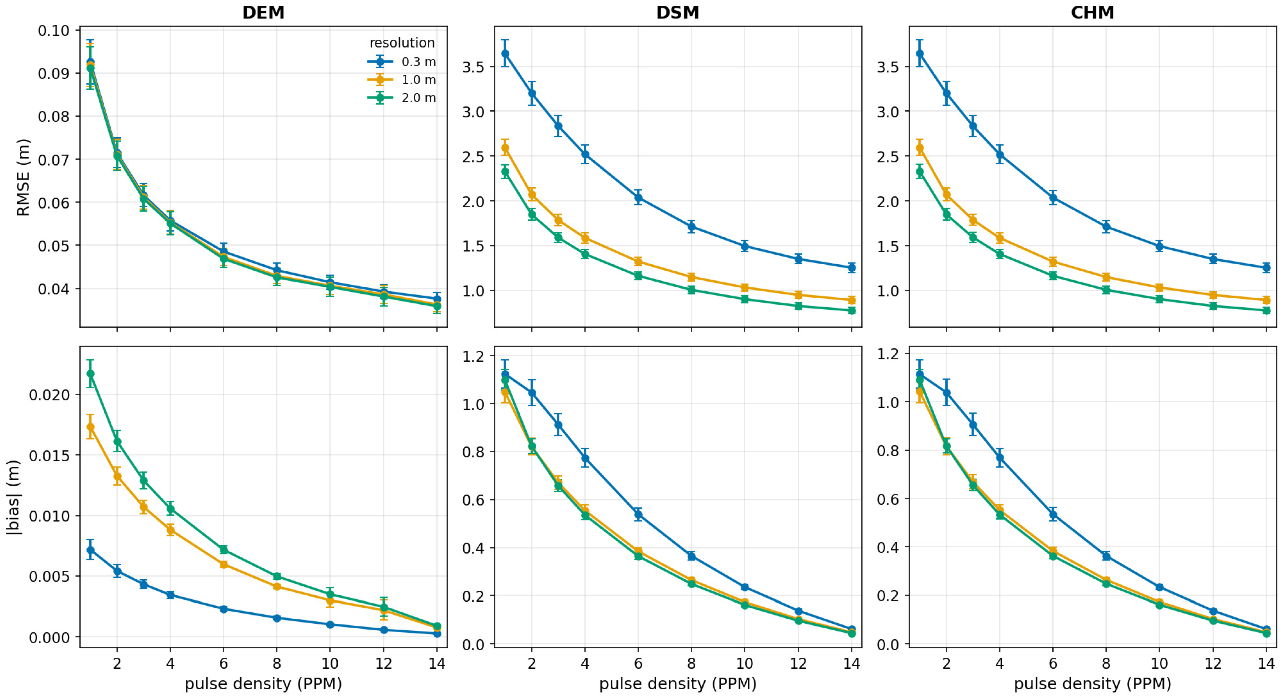
Our results demonstrated a strong relationship between ALS pulse density and elevation raster accuracy, particularly for DSMs and CHMs. Across all three spatial resolutions, increasing pulse density significantly reduced both absolute mean bias and tile-level RMSE for the DEM, DSM, and CHM. Mixed-effect models identified a highly significant overall relationship between pulse density and raster accuracy (fixed-effect slope, p < 0.001). Pairwise comparisons further showed that each successive increase in pulse density produced a significant reduction in RMSE (Holm-corrected p < 0.001), although the magnitude of improvement diminished at higher densities. For example, for the 0.3 m DSM, the median per-step RMSE reduction declined from approximately 0.44 m between 1 and 2 PPM to less than 0.10 m between 12 and 14 PPM. However, the practical effect varied considerably among raster types. DEM accuracy was relatively insensitive to pulse density, with mean tile RMSE decreasing only from approximately 0.09 m at 1 PPM to 0.04 m at 14 PPM and absolute bias remaining below 0.01 m. In contrast, DSM and CHM accuracy improved substantially, with mean tile RMSE at 0.3 m decreasing from approximately 3.6 m at 1 PPM to 1.25 m at 14 PPM. These overall trends are summarized in Figure 2.

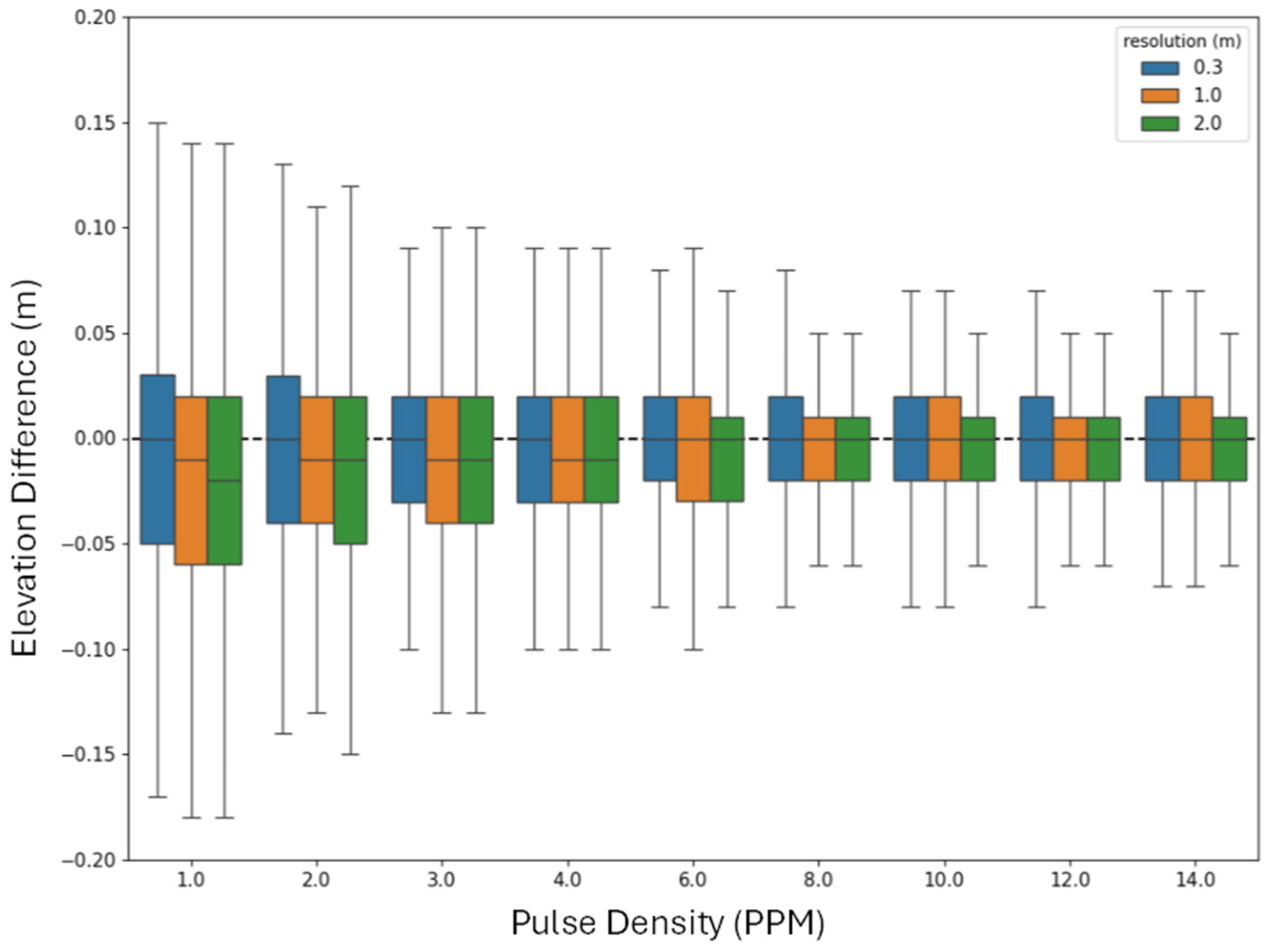
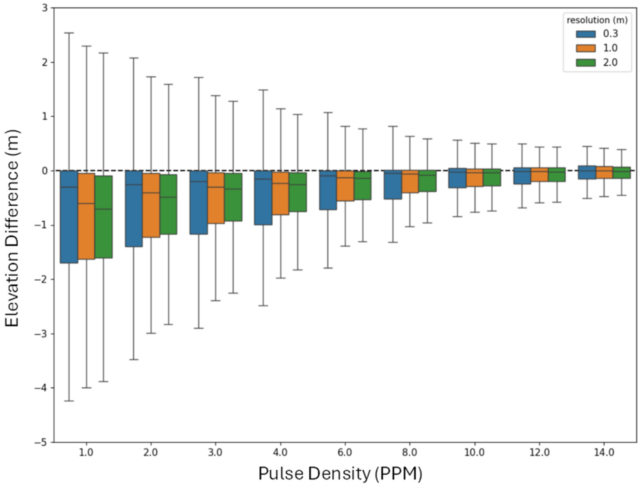
The DEMs exhibited minimal systematic error relative to the 16 PPM reference regardless of pulse density or spatial resolution (Figure 3). Although lower-density datasets (<8 PPM) showed a slight negative bias, elevation differences remained small and became progressively less variable with increasing pulse density. The range of elevation differences narrowed from approximately ±0.17 m at 1 PPM to ±0.07 m at 14 PPM, illustrating the consistently high stability of DEMs even at relatively sparse pulse densities.

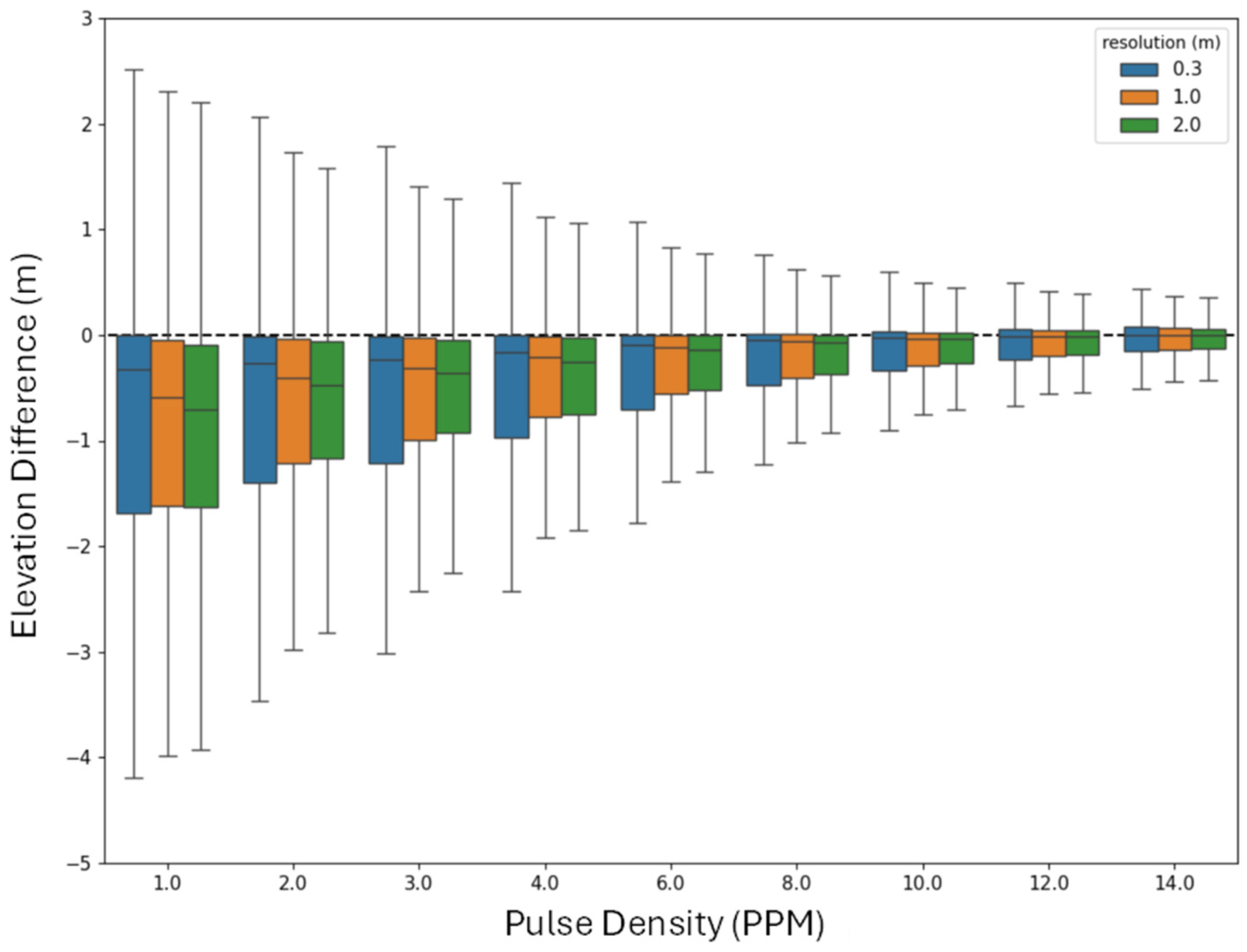
In contrast, DSMs and CHMs were considerably more sensitive to pulse density (Figure 4 and Figure 5). Both products exhibited pronounced negative bias in the sparsest datasets, reflecting increasing underestimation of canopy elevations as pulse density decreased. This bias steadily diminished with increasing pulse density, while the distributions of elevation differences became progressively narrower across all spatial resolutions. For DSMs, the spread of differences remained greater than ±1 m until approximately 8 PPM before contracting to roughly ±0.45 m by 14 PPM. CHMs followed nearly identical patterns, with both bias and variability decreasing consistently as pulse density increased.

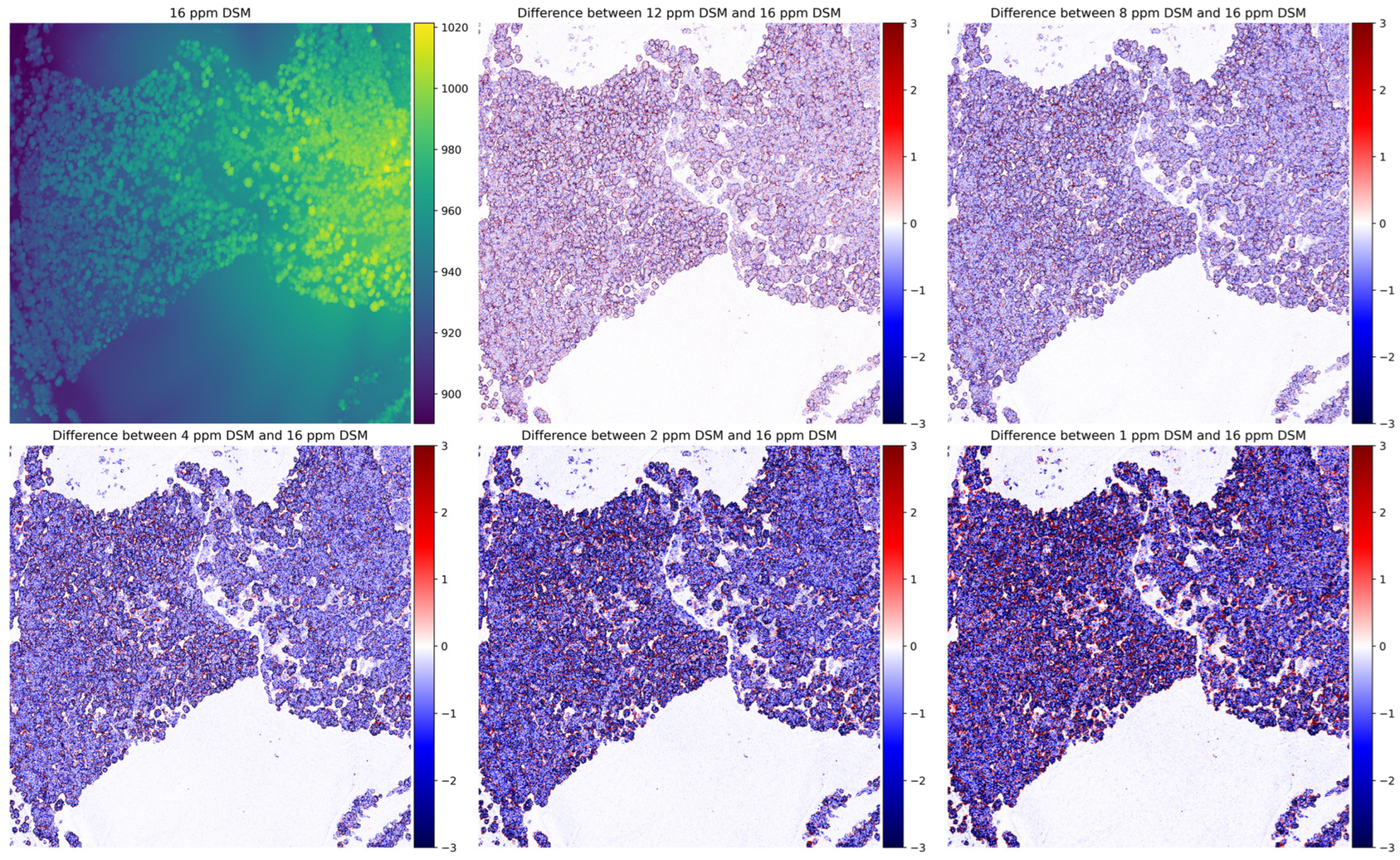
These patterns were expected, as CHMs are derived from both the DSM and DEM. Given the negligible bias observed in the DEM across pulse densities, it follows that CHM trends would strongly resemble those of the DSMs. As in the DSM analysis, CHM difference distributions did not drop below ±1 m until pulse densities reached 8 PPM. Beyond this point, the spread tightened further, reaching approximately ±0.45 m or less at 14 PPM. The reduction in bias for both DSMs and CHMs is visually illustrated further in Figure 6.

Across all three raster types (DEM, DSM, and CHM), the 2.0 m resolution consistently produced the narrowest difference distributions and smallest interquartile ranges at each pulse density. In contrast, the highest spatial resolution (0.3 m) generally exhibited the widest spreads and largest interquartile ranges for a given pulse density.

3.2. Effects of Pulse Density on Estimates of Tree Height

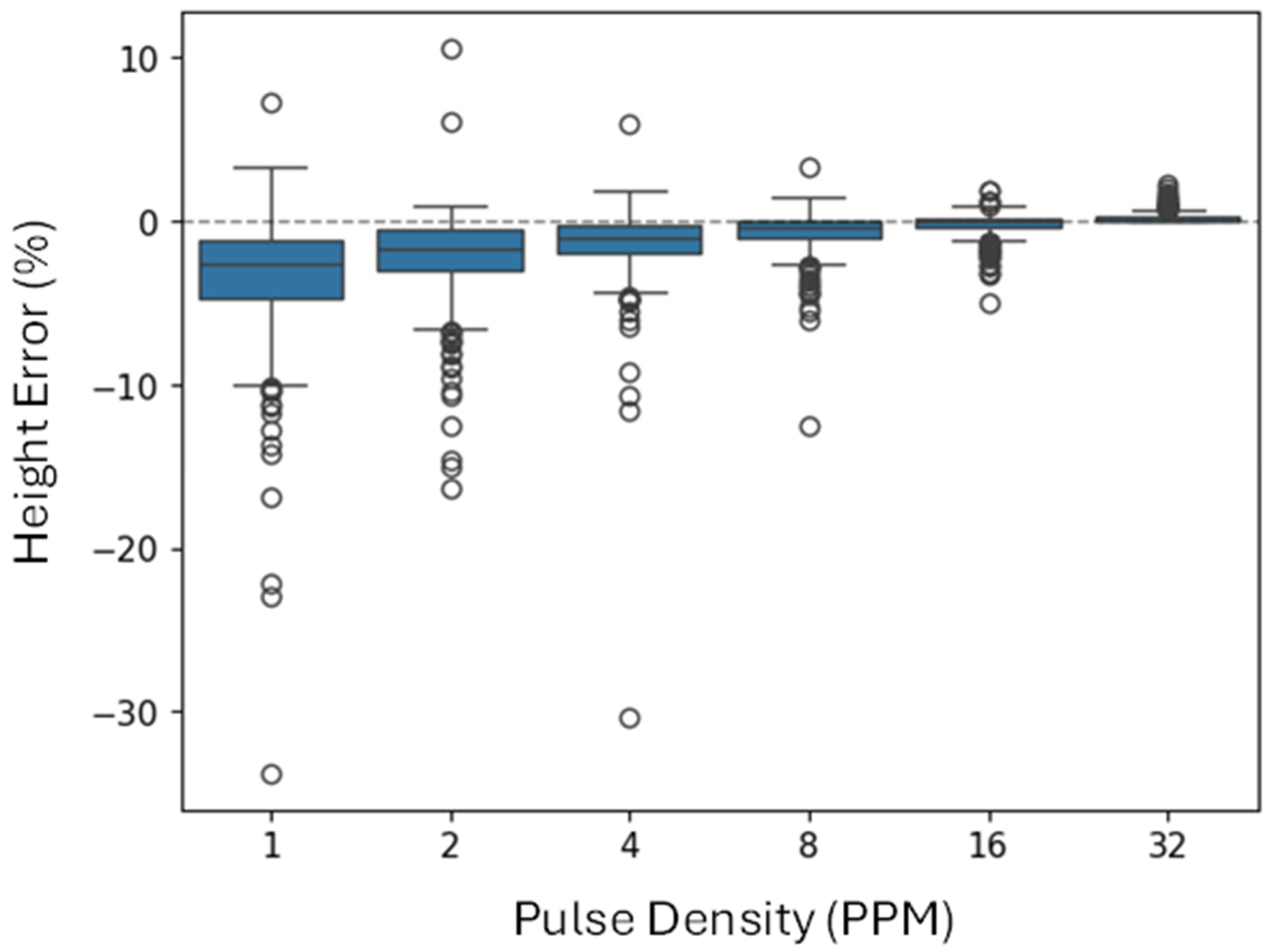
When looking at individual trees, the error in LiDAR-estimated heights relative to field measurements had an inverse relationship with pulse density—as pulse density increased, the error decreased. For sparser datasets, there was also an evident negative bias in the LiDAR heights—sparse datasets typically led to under-prediction of tree height (Figure 7).

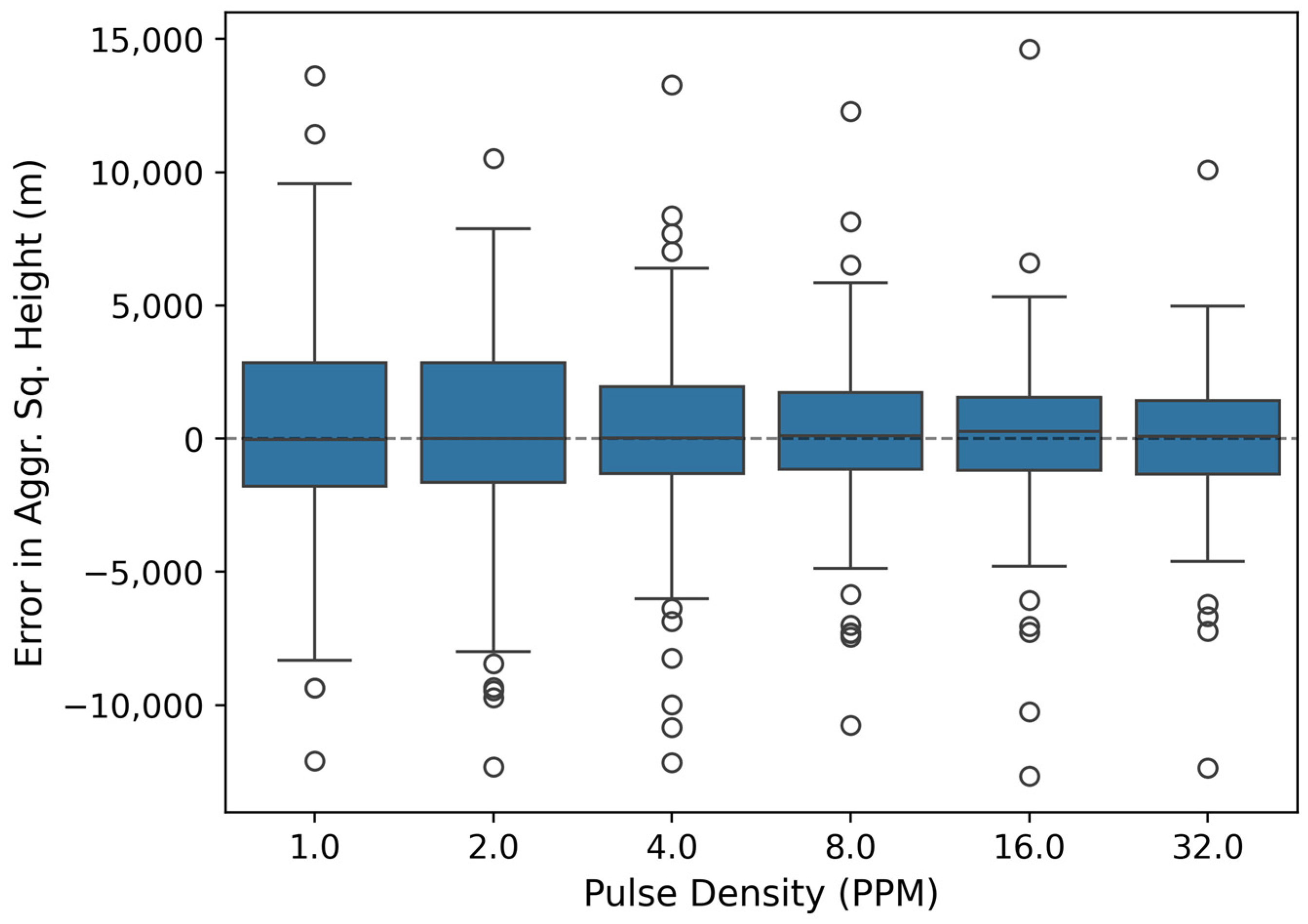
Similarly, when aggregating at the plot level, as pulse density increased, the error in squared height consistently decreased (Figure 8). Lower-density datasets exhibited higher variability in height estimates, leading to larger deviations from field-measured values. In contrast, higher-density datasets produced tighter error distributions and therefore more accurate and stable height measurements. This trend was observed across all sample plots, indicating improved structural representation of tree and canopy height with increased point density.

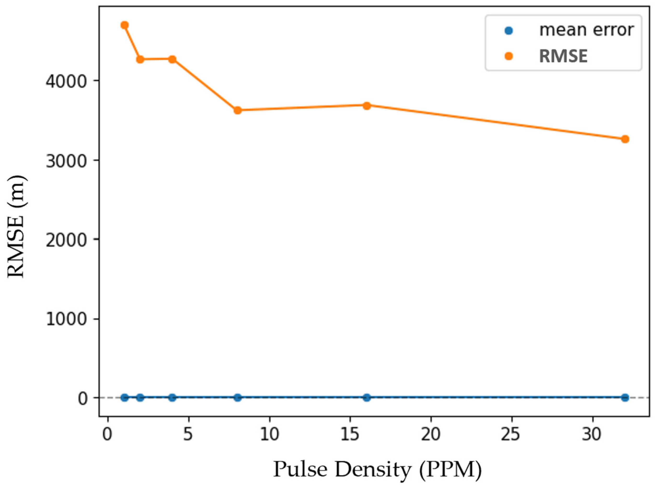
RMSE of aggregated squared tree height quickly decreased when increasing pulse density from 1 to 8 PPM (Figure 9). It then followed a gradual downward trajectory as pulse density continued to increase.

3.3. Visual Effects of Pulse Density on Individual Tree Definition

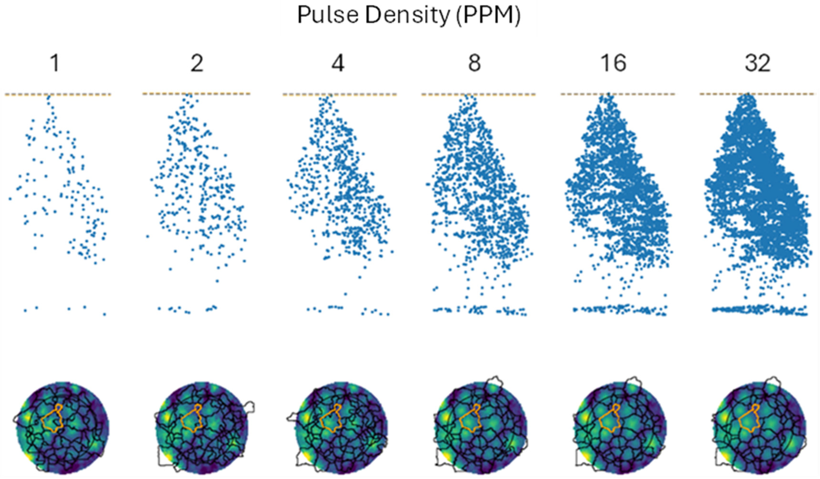
When analyzing the datasets subsampled from the original 36 PPM dataset, the effect of pulse density on the visualization of tree objects is clearly visible (Figure 10). Higher pulse densities result in a greater number of points in both the lower canopy and on the ground, improving the detail of the vertical structure of the forest. Tree crowns appear more defined, and vertical layering is more evident in higher-density datasets.

4. Discussion

This study investigated how pulse density influences the quality of derivative raster products—DEMs, DSMs, and CHMs—as well as ALS-derived tree height estimates. To assess these effects, we systematically thinned the original ALS point cloud to create datasets representing a range of pulse densities. For each thinned dataset, rasters were generated and compared against reference rasters derived from the 16 PPM dataset. Similarly, we evaluated ALS-derived tree heights across pulse densities ranging from 1 to 32 PPM and compared those values with field-measured tree heights. Processing workflows and parameters were deliberately kept constant across all tests to ensure that any observed differences could be directly attributed to variations in input pulse density rather than methodological inconsistencies. This controlled approach provided a clear basis for isolating and quantifying the effects of pulse density on both elevation model quality and tree height accuracy.

While many studies have examined the effects of data thinning on LiDAR-derived products, most have done so by reducing the number of points rather than pulses [34]. This distinction is critical because the number of returns per pulse can vary substantially within an ALS acquisition, and simply removing points does not accurately simulate a true change in pulse density. In this study, we reduced the number of pulses themselves, sampling pulses and their corresponding returns to achieve desired densities—an approach more consistent with an independent ALS acquisition. Our methods align most closely with those described by Watt (2013) [46], though we recognize that alternative approaches, such as those used by Wilkes et al. (2015) [34], may further refine these simulations. Our DEM analysis parallels the work of Anderson et al. (2006) [26], but with notable extensions. We employed substantially higher-density datasets and applied the same principles to DSMs and CHMs, allowing us to evaluate pulse density effects across multiple raster products. Additionally, we tested much finer spatial resolutions (0.3, 1, and 2 m) compared with Anderson et al.’s 5, 10, and 30 m scales. Compared to prior studies [25,26,33,34,47], we utilized considerably denser datasets—many earlier analyses were limited to <8 PPM, which was considered high-density at the time. Peng et al. (2021) [48] did examine high point densities (up to 108 points/m²), but their data were collected using a UAV platform. Given that ALS remains the preferred platform for large-scale operational forest inventory and shows promise for carbon quantifications [11], this study may serve as a more relevant, modernized evaluation of pulse density effects.

DEM accuracy showed minimal bias across all pulse densities tested. Although elevation variability decreased slightly as pulse density increased, overall results indicate that even relatively sparse ALS data can reliably characterize ground surfaces in forested environments. Our results align with those of Liu et al. (2007) [25], Anderson et al. (2006) [26], and Cățeanu et al. (2021) [49], all of whom reported minimal DEM sensitivity to pulse density. These findings suggest that low-density ALS data may be adequate for applications focused solely on ground modeling—such as terrain normalization prior to segmentation in ITD workflows. The dense canopy of the UIEF study area reinforces this conclusion and implies that results may generalize to other forest types, potentially with even greater accuracy in more open canopies where ground visibility improves.

In contrast, the benefits of higher pulse densities became increasingly evident in DSM and CHM outputs. These layers directly support ITD and other forest inventory workflows, and their accuracy strongly influences the quality of subsequent analyses. Insufficient pulse density can bias DSM and CHM heights downward, degrading segmentation accuracy and propagating errors throughout the inventory process. Consistent with the work of Silva et al. (2013) [28], we observed steady improvements in DSM and CHM accuracy with increasing pulse density. As density increased, canopy height underestimation diminished substantially, revealing a clear negative correlation. Because DSMs and CHMs form the basis for many forest remote sensing workflows—including ITD—their precision often determines the accuracy of derived metrics such as tree height, DBH, and biomass. As emphasized by Peng et al. (2021) [48], high-quality CHMs are essential for reliable tree height extraction. In short, accurate inputs yield accurate outputs.

This trend carries important implications for ALS specification design. In modern forest inventory systems with strict accuracy requirements, low-density data (<8 PPM) may be inadequate for generating reliable DSMs or CHMs. Height underestimation in these products can lead to misattributed tree heights and inaccurate downstream estimates of volume, crown dimensions, and biomass. Furthermore, because segmentation typically precedes attribute assignment, errors introduced by low-quality canopy models can compromise the entire workflow from the beginning. Our findings therefore underscore the advantage of acquiring high-density ALS data to ensure robust, bias-free canopy surface models and dependable segmentation inputs.

Tree height estimation accuracy followed a similar trend to that observed in the raster analyses. Subsampling the original 36 PPM dataset revealed a strong positive relationship between pulse density and tree height accuracy. As pulse density increased, deviations from field-measured heights decreased, and bias was largely eliminated. These improvements are attributable to the increased probability of sufficiently capturing treetop and ground returns, both of which are critical components for accurate height measurement. This effect is particularly pronounced in structurally complex forests like the UIEF, where dense canopy closure and multilayered vegetation often obscure both canopy peaks and ground points in low-density data.

These findings have important implications, as accurate tree height estimates underpin a wide range of forest inventory metrics—DBH, basal area, volume, and biomass—as well as related processes, including growth and yield modeling, harvest scheduling, and carbon project development. Specifically in terms of biomass estimation, if using a carbon registry-approved biomass model like those produced by Woodall et al. 2011 [32] that uses height as an input, lower quality LiDAR datasets could negatively impact resulting biomass estimates. In such instances, more accurate tree heights resulting from higher-density data would be preferred. Systematic height underestimation in low-density datasets not only biases height itself but propagates through entire modeling pipelines, introducing widespread error. Additionally, improved height accuracy can enhance repeat-scan analyses for monitoring growth, site productivity, and carbon flux. With higher baseline accuracy, change detection becomes more sensitive and reliable over time. We also observed qualitative improvements in the visualization of canopy structures as pulse density increased—denser point clouds produced more distinct crowns and reduced ambiguity between neighboring trees. Although we did not explicitly evaluate ITD performance, these improvements in point cloud definition likely enhance segmentation accuracy in workflows using cloud-based or hybrid methods [50].

It is worth noting that while field-measured heights served as our validation reference, previous studies [31] have shown that LiDAR-derived heights can surpass field measurements in accuracy. This can be especially true for conical shaped tree species, which dominate the UIEF study area. Confidence in these comparisons could be further enhanced through more rigorous validation methods such as a felled-tree analysis similar to those performed by Sibona et al. (2016) [31] and Sparks et al. (2024) [51]. Ultimately, the optimal pulse density depends on project objectives. For tasks requiring only DEM generation, lower-density data may suffice. However, for applications with low error tolerance in height estimation or those requiring high-fidelity canopy representations—such as tree segmentation and comprehensive forest inventories—our findings support the use of higher pulse densities to ensure accurate and reliable outcomes.

5. Conclusions

The purpose of this study was to provide clear guidance for forestry practitioners, natural resource managers, and carbon project stakeholders, emphasizing key insights into the utility and operational considerations of airborne LiDAR systems for forest inventory and biomass assessment. Specifically, we aimed to demonstrate the potential benefits of acquiring higher-density airborne laser scanning (ALS) data while also highlighting the risks associated with using lower-density datasets in forest inventory and carbon quantification applications. Beyond forest inventory and carbon quantification, our results may also add value to other biomass-related applications, such as hazardous fuel assessments in which improved tree height accuracy could enhance fuel loading estimates, therefore supporting more effective wildfire risk mitigation efforts.

To conduct this study, we subsampled a high-density ALS dataset into multiple lower-density datasets which were then pushed through the ForestView^® ALS processing pipeline to create key raster products commonly used in ITD segmentation workflows—specifically, DEMs, DSMs, and CHMs. Outputs were evaluated for accuracy by comparing them to rasters derived from a 16 PPM dataset. Additionally, we segmented and attributed individual tree objects, and then validated ALS-derived tree heights against field-measured values.

DSM and CHM quality improved with higher densities, producing rasters that more closely represented true canopy structure. Conversely, DEM accuracy was relatively stable across all tested densities, suggesting that lower-density data (e.g., ≤8 PPM) may often suffice for ground surface modeling applications in forested environments. However, using such low-density data for generating DSMs and CHMs introduces a consistent negative bias in canopy height estimates, which can compromise the reliability of subsequent forest inventory metrics. Our findings also revealed a clear positive relationship between pulse density and the accuracy of ALS-derived tree heights. As pulse density increased, tree height estimates and downstream outputs such as volume and biomass became more accurate with reduced variability and bias.

Looking ahead, there remains significant opportunity for continued research, innovation, and cost efficiencies. What constitutes “high-density” is constantly being redefined as LiDAR technology advances. Pulse densities once considered cutting-edge now fall short of modern standards, underscoring the need to continually evaluate and push the capabilities of current systems. With data acquisition costs being a leading decision factor for most forest inventory and carbon accounting efforts, understanding the potential efficiencies offered by new and/or evolving technology is paramount. For example, future research should investigate emerging technologies such as Geiger-mode LiDAR, which has the potential to deliver high-resolution data collection from greater altitudes. However, these systems pose new challenges due to incompatibility with traditional linear-mode processing workflows. Developing new methods to process and integrate Geiger-mode data will be critical to unlocking new potential and ensuring alignment with existing forestry data infrastructures.

References

1. Burkhart, H.E.; Avery, T.H.; Bullock, B.P. Forest Measurements, 5th ed.; Waveland Press: Long Grove, IL, USA, 2015; pp. 34–70. [Google Scholar]
2. Schreuder, H.T.; Gregoire, T.G.; Wood, G.B. Sampling Methods for Multiresource Forest Inventory; John Wiley & Sons, Inc.: New York, NY, USA, 1993; pp. 111–158. [Google Scholar]
3. Booth, D.T.; Cox, S.E.; Meikle, T.; Zuuring, H.R. Ground-cover measurements: Assessing correlation among aerial and ground-based methods. Environ. Manag. 2008, 42, 1091–1100. [Google Scholar] [CrossRef] [PubMed]
4. Mäkinen, A.; Kangas, A.; Nurmi, M. Using cost-plus-loss analysis to define optimal forest inventory interval and forest inventory accuracy. Silva Fenn. 2012, 46, 211–226. [Google Scholar] [CrossRef]
5. Hetzer, J.; Huth, A.; Wiegand, T.; Dobner, H.J.; Fischer, R. An analysis of forest biomass sampling strategies across scales. Biogeosciences 2020, 17, 1673–1683. [Google Scholar] [CrossRef]
6. Cunia, T. Some theory on reliability of volume estimates in a forest inventory sample. For. Sci. 1965, 11, 115–128. [Google Scholar] [CrossRef]
7. Scott, C.T. Sampling methods for estimating change in forest resources. Ecol. Appl. 1998, 8, 228–233. [Google Scholar] [CrossRef]
8. Lefsky, M.A.; Cohen, W.B.; Parker, G.G.; Harding, D.J. Lidar Remote Sensing for Ecosystem Studies. BioScience 2002, 52, 19–30. [Google Scholar] [CrossRef]
9. Beland, M.; Parker, G.; Sparrow, B.; Harding, D.; Chasmer, L.; Phinn, S.; Antonarakis, A.; Strahler, A. On promoting the use of lidar systems in forest ecosystem research. For. Ecol. Manag. 2019, 450, 117484. [Google Scholar] [CrossRef]
10. Wehr, A.; Lohr, U. Airborne laser scanning—An introduction and overview. ISPRS J. Photogramm. Remote Sens. 1999, 54, 68–82. [Google Scholar] [CrossRef]
11. Corrao, M.; Wimme, L.; Butler, J.; Glaze, J.; Latta, G.; Trierweiler, D. Airborne Laser Scanning for Large-Scale Forest Carbon Quantification: A Comparison of LiDAR Single-Tree and Field-Based Methods. Remote Sens. 2026, 18, 547. [Google Scholar] [CrossRef]
12. Balestra, M.; Marselis, S.; Sankey, T.T.; Cabo, C.; Liang, X.; Mokroš, M.; Peng, X.; Singh, A.; Stereńczak, K.; Vega, C.; et al. LiDAR Data Fusion to Improve Forest Attribute Estimates: A Review. Curr. For. Rep. 2024, 10, 281–297. [Google Scholar] [CrossRef]
13. Hummel, S.; Hudak, A.T.; Uebler, E.H.; Falkowski, M.J.; Megown, K.A. A comparison of accuracy and cost of LiDAR versus stand exam data for landscape management on the Malheur National Forest. J. For. 2011, 109, 267–273. [Google Scholar] [CrossRef]
14. Reutebuch, S.E.; Andersen, H.E.; McGaughey, R.J. Light detection and ranging (LIDAR): An emerging tool for multiple resource inventory. J. For. 2005, 103, 286–292. [Google Scholar] [CrossRef]
15. Montzka, T.; Scharosch, S.; Huebschmann, M.; Corrao, M.V.; Hardman, D.D.; Rainsford, S.W.; Smith, A.M.S. The Confederated Tribes and Bands of the Yakama Nation; Comparison of a Continuous Forest Inventory to an ALS-Derived Digital Inventory in Washington State. Remote Sens. 2025, 17, 1761. [Google Scholar] [CrossRef]
16. Kaartinen, H.; Hyyppä, J.; Yu, X.; Vastaranta, M.; Hyyppä, H.; Kukko, A.; Holopainen, M.; Heipke, C.; Hirschmugl, M.; Morsdorf, F.; et al. An international comparison of individual tree detection and extraction using airborne laser scanning. Remote Sens. 2012, 4, 950–974. [Google Scholar] [CrossRef]
17. Parkitna, K.; Krok, G.; Miścicki, S.; Ukalski, K.; Lisańczuk, M.; Mitelsztedt, K.; Magnussen, S.; Markiewicz, A.; Stereńczak, K. Modelling growing stock volume of forest stands with various ALS area-based approaches. Forestry 2021, 94, 630–650. [Google Scholar] [CrossRef]
18. van Lier, O.R.; Luther, J.E.; White, J.C.; Fournier, R.A.; Côté, J.F. Effect of scan angle on ALS metrics and area-based predictions of forest attributes for balsam fir dominated stands. Forestry 2022, 95, 49–72. [Google Scholar] [CrossRef]
19. Sparks, A.M.; Corrao, M.V.; Smith, A.M. Cross-comparison of individual tree detection methods using low and high pulse density airborne laser scanning data. Remote Sens. 2022, 14, 3480. [Google Scholar] [CrossRef]
20. Jakubowski, M.K.; Li, W.; Guo, Q.; Kelly, M. Delineating individual trees from LiDAR data: A comparison of vector-and raster-based segmentation approaches. Remote Sens. 2013, 5, 4163–4186. [Google Scholar] [CrossRef]
21. Roussel, J.R.; Auty, D.; Coops, N.C.; Tompalski, P.; Goodbody, T.R.; Meador, A.S.; Bourdon, J.-F.; de Boissieu, F.; Achim, A. lidR: An R package for analysis of Airborne Laser Scanning (ALS) data. Remote Sens. Environ. 2020, 251, 112061. [Google Scholar] [CrossRef]
22. Diószegi, G.; Molnár, V.É.; Nagy, L.A.; Enyedi, P.; Török, P.; Szabó, S. A new method for individual treetop detection with low-resolution aerial laser scanned data. Model. Earth Syst. Environ. 2024, 10, 5225–5240. [Google Scholar] [CrossRef]
23. R Core Team. A Language and Environment for Statistical Computing; R Foundation for Statistical Computing: Vienna, Austria, 2025; Available online: https://www.R-project.org (accessed on 11 November 2025).
24. Corrao, M.V.; Sparks, A.M.; Smith, A.M.S. A Conventional Cruise and Felled-Tree Validation of Individual Tree Diameter, Height and Volume Derived from Airborne Laser Scanning Data of a Loblolly Pine (P. taeda) Stand in Eastern Texas. Remote Sens. 2022, 14, 2567. [Google Scholar] [CrossRef]
25. Liu, X.; Zhang, Z.; Peterson, J.; Chandra, S. The effect of LiDAR data density on DEM accuracy. In Proceedings of the 17th International Congress on Modelling and Simulation (MODSIM07), Christchurch, New Zealand, 10–13 December 2007. [Google Scholar]
26. Anderson, E.S.; Thompson, J.A.; Crouse, D.A.; Austin, R.E. Horizontal resolution and data density effects on remotely sensed LIDAR-based DEM. Geoderma 2006, 132, 406–415. [Google Scholar] [CrossRef]
27. Silva, C.A.; Hudak, A.T.; Vierling, L.A.; Klauberg, C.; Garcia, M.; Ferraz, A.; Keller, M.; Eitel, J.; Saatchi, S. Impacts of airborne lidar pulse density on estimating biomass stocks and changes in a selectively logged tropical forest. Remote Sens. 2017, 9, 1068. [Google Scholar] [CrossRef]
28. Silva, C.A.; Hudak, A.; Liebermann, R.; Satterberg, K.; Rodriguez, L.C.E. Evaluation of digital elevation models (DEMs) from high and low pulse density in LiDAR data. In Proceedings of the 16th Brazilian Symposium on Remote Sensing—SBSR, Foz do Iguaçu, Brazil, 13–18 April 2013. [Google Scholar]
29. Filipescu, C.N.; Groot, A.; MacIsaac, D.A.; Cruickshank, M.G.; Stewart, J.D. Prediction of diameter using height and crown attributes: A case study. West. J. Appl. For. 2012, 27, 30–35. [Google Scholar] [CrossRef]
30. Vauhkonen, J.; Korpela, I.; Maltamo, M.; Tokola, T. Imputation of single-tree attributes using airborne laser scanning-based height, intensity, and alpha shape metrics. Remote Sens. Environ. 2010, 114, 1263–1276. [Google Scholar] [CrossRef]
31. Sibona, E.; Vitali, A.; Meloni, F.; Caffo, L.; Dotta, A.; Lingua, E.; Motta, R.; Garbarino, M. Direct measurement of tree height provides different results on the assessment of LiDAR accuracy. Forests 2016, 8, 7. [Google Scholar] [CrossRef]
32. Woodall, C.W.; Heath, L.S.; Domke, G.M.; Nichols, M.C. Methods and Equations for Estimating Aboveground Volume, Biomass, and Carbon for Trees in the U.S. Forest Inventory, 2010; General Technical Report NRS-88; US Department of Agriculture, Forest Service, Northern Research Station: Newtown Square, PA, USA, 2011; Volume 88, pp. 1–30. [CrossRef]
33. Zhao, K.; Suarez, J.C.; Garcia, M.; Hu, T.; Wang, C.; Londo, A. Utility of multitemporal lidar for forest and carbon monitoring: Tree growth, biomass dynamics, and carbon flux. Remote Sens. Environ. 2018, 204, 883–897. [Google Scholar] [CrossRef]
34. Wilkes, P.; Jones, S.D.; Suarez, L.; Haywood, A.; Woodgate, W.; Soto-Berelov, M.; Mellor, A.; Skidmore, A.K. Understanding the effects of ALS pulse density for metric retrieval across diverse forest types. Photogramm. Eng. Remote Sens. 2015, 81, 625–635. [Google Scholar] [CrossRef]
35. Kwak, D.A.; Lee, W.K.; Lee, J.H.; Biging, G.S.; Gong, P. Detection of individual trees and estimation of tree height using LiDAR data. J. For. Res. 2007, 12, 425–434. [Google Scholar] [CrossRef]
36. Suárez, J.C.; Ontiveros, C.; Smith, S.; Snape, S. Use of airborne LiDAR and aerial photography in the estimation of individual tree heights in forestry. Comput. Geosci. 2005, 31, 253–262. [Google Scholar] [CrossRef]
37. United States Geological Survey. Lidar Base Specification 2025 Rev. A. Available online: https://www.usgs.gov/media/files/lidar-base-specification-2025-rev-a (accessed on 11 November 2025).
38. Cosgrove, C.F.; Coops, N.C.; Martin, T.G. Using the full potential of Airborne Laser Scanning (aerial LiDAR) in wildlife research. Wildl. Soc. Bull. 2024, 48, e1532. [Google Scholar] [CrossRef]
39. Siddiqui, T.; Alveshere, B.; Gough, C.; van Aardt, J.; Krause, K. Modeling Primary Production in Temperate Forests Using Three-Dimensional Canopy Structural Complexity Metrics Derived from Airborne LiDAR Data. Remote Sens. 2025, 17, 2817. [Google Scholar] [CrossRef]
40. Roussel, J.R.; Caspersen, J.; Béland, M.; Thomas, S.; Achim, A. Removing bias from LiDAR-based estimates of canopy height: Accounting for the effects of pulse density and footprint size. Remote Sens. Environ. 2017, 198, 1–16. [Google Scholar] [CrossRef]
41. SOMAG Jena Germany. Gyro Stabilization Mount (GSM) 4000 [WWW Document]. 2022. Available online: https://www.somag-ag.de/products/airborne-gyro-mounts/gsm-4000/ (accessed on 15 April 2026).
42. Riegl USA. RiPROCESS [WWW Document]. 2022. Available online: http://www.rieglusa.com/index.html (accessed on 15 April 2026).
43. Popescu, S.C.; Wynne, R.H. Seeing the trees in the forest: Using lidar and multispectral data fusion with local filtering and variable window size for estimating tree height. Photogramm. Eng. Remote Sens. 2004, 70, 589–604. [Google Scholar] [CrossRef]
44. Sparks, A.M.; Smith, A.M. Accuracy of a lidar-based individual tree detection and attribute measurement algorithm developed to inform forest products supply chain and resource management. Forests 2021, 13, 3. [Google Scholar] [CrossRef]
45. Xu, Q.; Li, B.; Maltamo, M.; Tokola, T.; Hou, Z. Predicting tree diameter using allometry described by non-parametric locally-estimated copulas from tree dimensions derived from airborne laser scanning. For. Ecol. Manag. 2019, 434, 205–212. [Google Scholar] [CrossRef]
46. Watt, M.S.; Adams, T.; Gonzalez Aracil, S.; Marshall, H.; Watt, P. The influence of LiDAR pulse density and plot size on the accuracy of New Zealand plantation stand volume equations. N. Z. J. For. Sci. 2013, 43, 15. [Google Scholar] [CrossRef]
47. Tesfamichael, S.G.; Van Aardt, J.A.N.; Ahmed, F. Estimating plot-level tree height and volume of Eucalyptus grandis plantations using small-footprint, discrete return lidar data. Prog. Phys. Geogr. 2010, 34, 515–540. [Google Scholar] [CrossRef]
48. Peng, X.; Zhao, A.; Chen, Y.; Chen, Q.; Liu, H. Tree height measurements in degraded tropical forests based on UAV-LiDAR data of different point cloud densities: A case study on Dacrydium pierrei in China. Forests 2021, 12, 328. [Google Scholar] [CrossRef]
49. Cățeanu, M.; Ciubotaru, A. The effect of lidar sampling density on DTM accuracy for areas with heavy forest cover. Forests 2021, 12, 265. [Google Scholar] [CrossRef]
50. Wang, Y.; Hyyppä, J.; Liang, X.; Kaartinen, H.; Yu, X.; Lindberg, E.; Holmgren, J.; Qin, Y.; Mallet, C.; Ferraz, A.; et al. International benchmarking of the individual tree detection methods for modeling 3-D canopy structure for silviculture and forest ecology using airborne laser scanning. IEEE Trans. Geosci. Remote Sens. 2016, 54, 5011–5027. [Google Scholar] [CrossRef]
51. Sparks, A.M.; Corrao, M.V.; Keefe, R.F.; Armstrong, R.; Smith, A.M. An accuracy assessment of field and airborne laser scanning–derived individual tree inventories using felled tree measurements and log scaling data in a mixed conifer forest. For. Sci. 2024, 70, 228–241. [Google Scholar] [CrossRef]
Figure 1. 95% canopy height across the UIEF study area located in northern Idaho, USA. Sample plot locations used for this study are marked with a yellow X. Areas used for the raster analysis are marked with red crosshatch.
Forests 17 00878 g001
Figure 2. Mean tile-level raster error with respective 95% confidence intervals across the tested pulse densities.
Forests 17 00878 g002
Figure 3. Distribution of ground-elevation measurements from DEMs that were generated with different pulse densities and spatial resolutions. Measurements are relative to baseline values derived from a 16 ppm resampled cloud.
Forests 17 00878 g003
Figure 4. Distribution of canopy-elevation measurements from DSMs that were generated with different pulse densities and spatial resolutions. Measurements are relative to baseline values derived from a 16 ppm resampled cloud.
Forests 17 00878 g004
Figure 5. Distribution of canopy-height measurements from CHMs that were generated with different pulse densities and spatial resolutions. Measurements are relative to baseline values derived from a 16 ppm resampled cloud.
Forests 17 00878 g005
Figure 6. These images show the difference between a 16-ppm derived baseline DSM and DSMs generated from increasingly sparse cloud inputs. Negative DSM bias increases as the DSMs are generated from increasingly sparse clouds. We observed the same trend for CHMs.
Forests 17 00878 g006
Figure 7. Relative error in LiDAR tree heights in relation to field measured heights compared across pulse densities.
Forests 17 00878 g007
Figure 8. Error of plot-level aggregated squared ALS tree height estimates relative to field measurements across various pulse densities.
Forests 17 00878 g008
Figure 9. RMSE of aggregated squared tree height across pulse densities. Height estimates for different pulse densities were rescaled to eliminate measurement bias, isolating impacts on the RMSE.
Forests 17 00878 g009
Figure 10. Visual change in point cloud density, definition of tree architecture, understory vegetation, and representation of ground surface resulting from increased pulse density.
Forests 17 00878 g010
Disclaimer/Publisher’s Note: The statements, opinions and data contained in all publications are solely those of the individual author(s) and contributor(s) and not of MDPI and/or the editor(s). MDPI and/or the editor(s) disclaim responsibility for any injury to people or property resulting from any ideas, methods, instructions or products referred to in the content.