Article

Forest Carbon Stock Dynamics in the West Qinling Mountains (2000–2025): A Multi-Source Remote Sensing Assessment with Spatial Robustness and Scenario Uncertainty

1
College of Bioengineering and Technology, Tianshui Normal University, Tianshui 741001, China
2
Key Laboratory of Resource Utilization of Agricultural Solid Waste in Gansu Province, Tianshui Normal University, Tianshui 741001, China
3
College of Resources and Environmental Engineering, Tianshui Normal University, Tianshui 741001, China
*
Author to whom correspondence should be addressed.
Forests 2026, 17(8), 867; https://doi.org/10.3390/f17080867
Submission received: 12 June 2026 / Revised: 17 July 2026 / Accepted: 23 July 2026 / Published: 24 July 2026
(This article belongs to the Section Forest Ecology and Management)

Abstract

This study develops a workflow for forest carbon accounting in the West Qinling Mountains, China (2000–2025), integrating CLCD data, key-year forest subtype mapping, and InVEST-style carbon pools. Forest subtypes were classified with Random Forest under spatial block cross-validation (overall accuracy = 59.76%, Cohen’s Kappa = 0.3974, Macro-F1 = 0.5944). Under the baseline workflow, total carbon stock increased from 876.40 to 954.45 million Mg C, yielding a net gain of 78.05 million Mg C (+8.91%). The Hamed–Rao modified Mann–Kendall test identified a significant increase (Sen’s slope = 2.41 million Mg C year−1, p = 2.99 × 10 5 ). A bounded parameter sensitivity analysis produced a 2025 total carbon range of 887.07–1021.84 million Mg C, whereas Scheme A yielded a more conservative net gain of 60.19 million Mg C. County-level patterns were broadly similar across scenarios, but fine-grained ranking remained uncertain. Because the annual series is a hybrid product, with annual forest/non-forest updates but a subtype structure refreshed only at key years, the results should not be interpreted as an independently reconstructed annual record of subtype transitions. The workflow therefore provides an uncertainty-aware regional accounting framework rather than a fully observed annual reconstruction of historical forest composition.

1. Introduction

The global carbon cycle is strongly mediated by terrestrial ecosystems, including forests, which constitute the largest and most dynamic carbon pool on land. Forests sequester atmospheric carbon dioxide through photosynthesis and store it in living biomass, dead organic matter, and soils, thereby moderating the effects of anthropogenic greenhouse gas emissions [1,2]. However, their capacity to function as carbon sinks is highly heterogeneous and sensitive to both natural disturbance and human intervention [3]. Understanding the spatiotemporal dynamics of forest carbon stocks is therefore critical for climate mitigation frameworks such as the Paris Agreement and the United Nations Framework Convention on Climate Change (UNFCCC). In China, large-scale ecological restoration programs over recent decades, notably, the Grain for Green Program (GGP) and the Natural Forest Protection Program (NFPP), have substantially expanded forest cover, making China’s terrestrial ecosystems an important component of the global carbon sink [4,5,6,7].
Despite these broad successes, precise quantification of forest carbon dynamics at regional scales remains challenging, especially in complex mountain ecosystems. Mountain regions such as the West Qinling Mountains in northwestern China are characterized by steep environmental gradients and highly diverse, fragmented forest landscapes [8]. These areas often function as critical ecological barriers and biodiversity hotspots, yet their carbon dynamics are difficult to monitor using traditional field inventories because of limited accessibility and strong spatial heterogeneity [9]. Remote sensing has therefore become indispensable for large-scale forest monitoring by providing continuous synoptic observations of land surface change.
Recent advances in remote sensing, especially the availability of long-term high-resolution satellite archives such as Landsat, have enabled detailed land cover time series. Products such as the annual China Land Cover Dataset (CLCD) provide unprecedented opportunities to track long-term land use trajectories at 30 m spatial resolution [10,11]. However, a major limitation of broad-scale land cover products for carbon accounting is their reliance on generic aggregated classes, such as a single “Forest” category. This simplification overlooks the structural, compositional, and functional heterogeneity among forest types. Broadleaf, coniferous, and mixed forests, for example, differ substantially in growth rate, stand structure, and equilibrium carbon density [12,13]. Treating these distinct ecosystems as a single homogeneous unit can bias regional carbon baselines and obscure the ecological consequences of forest succession and management intervention [14].
To overcome the limitations of generic forest classifications, machine learning algorithms have been increasingly employed to map forest subtypes using multi-source remote sensing data. Random Forests (RFs), in particular, have demonstrated exceptional performance in complex classification tasks due to their robustness against overfitting and ability to handle high-dimensional, non-parametric feature spaces [15]. By integrating spectral, textural, thermal, and topographic features, RF models can effectively distinguish between fine-grained forest categories [13,16,17,18]. However, the application of machine learning in remote sensing is frequently plagued by spatial autocorrelation, a phenomenon where geographic proximity leads to statistical dependence among observations. Standard random holdout validation strategies fail to account for this spatial structure, resulting in overly optimistic accuracy estimates that do not reflect the model’s true generalizability to unseen geographic areas. Rigorous spatial block cross-validation is therefore imperative to ensure the reliability of forest subtype maps [19,20,21].
When combined with accurate land cover maps, ecosystem service models such as the InVEST (Integrated Valuation of Ecosystem Services and Tradeoffs) Carbon Storage and Sequestration model provide a standardized framework for converting land use data into carbon stock estimates [22,23]. The InVEST model relies on land use-specific carbon density parameters across four fundamental pools: aboveground biomass, belowground biomass, soil organic carbon, and dead organic matter. Although this approach is highly scalable and transparent, its deterministic structure means that the final estimates depend strongly on the precision of the input parameter tables. Given the inherent variability of carbon density even within a single forest subtype, deterministic point estimates should be accompanied by explicit uncertainty and sensitivity analyses to provide credible carbon stock intervals [24,25,26]. This information is particularly important for decision-makers who need defensible bounds on carbon sink capacity when evaluating carbon trading mechanisms and emission reduction targets.
Despite recent Qinling-focused studies [27,28,29,30], practical gaps remain in how annual land cover continuity, subtype differentiation, and uncertainty communication are combined for decision support carbon accounting in the West Qinling context. In particular, annual continuity is much easier to support for a forest/non-forest mask than for historical forest subtype composition reconstructed under temporal transfer. The central contribution of this study is therefore a structurally constrained and uncertainty-aware regional carbon accounting workflow for a complex mountain region rather than a fully observed annual reconstruction of historical forest subtypes. The novelty of the study does not lie in inventing a new classifier or a new carbon model in isolation; instead, it lies in explicitly integrating subtype-resolved mapping, spatially explicit validation, key-year inheritance, and separated uncertainty reporting into a single regional accounting workflow whose assumptions are stated directly rather than left implicit. Specifically, the workflow integrates three components: (i) spatially validated forest subtype mapping that disaggregates the generic forest class into coniferous, broadleaf, and mixed forests; (ii) a key-year temporal consistency strategy (Scheme A) that preserves annual CLCD forest/non-forest dynamics while updating subtype structure only at key years; and (iii) a multi-component uncertainty framework that separately reports parameter sensitivity, classification uncertainty, and structural sensitivity for county-level interpretation. Against this background, we test the hypothesis that accounting for forest subtype composition can alter regional carbon stock baselines while broader regional accumulation patterns remain directionally similar under bounded parameter sensitivity, subject to the limitations of temporal subtype transfer. To operationalize this framework, we pursue four objectives: (i) to construct key-year forest subtype maps under spatially explicit validation and integrate them with annual CLCD masks under explicit structural constraints; (ii) to quantify total and density-based carbon dynamics using localized InVEST-style four-pool parameters; (iii) to summarize major subtype-resolved transition pathways as structurally inferred evidence of carbon change allocation rather than as direct annual observations of succession; and (iv) to report parameter, classification, and structural uncertainty in a form suitable for cautious county-level comparison.

2. Materials and Methods

2.1. Study Area and Data Sources

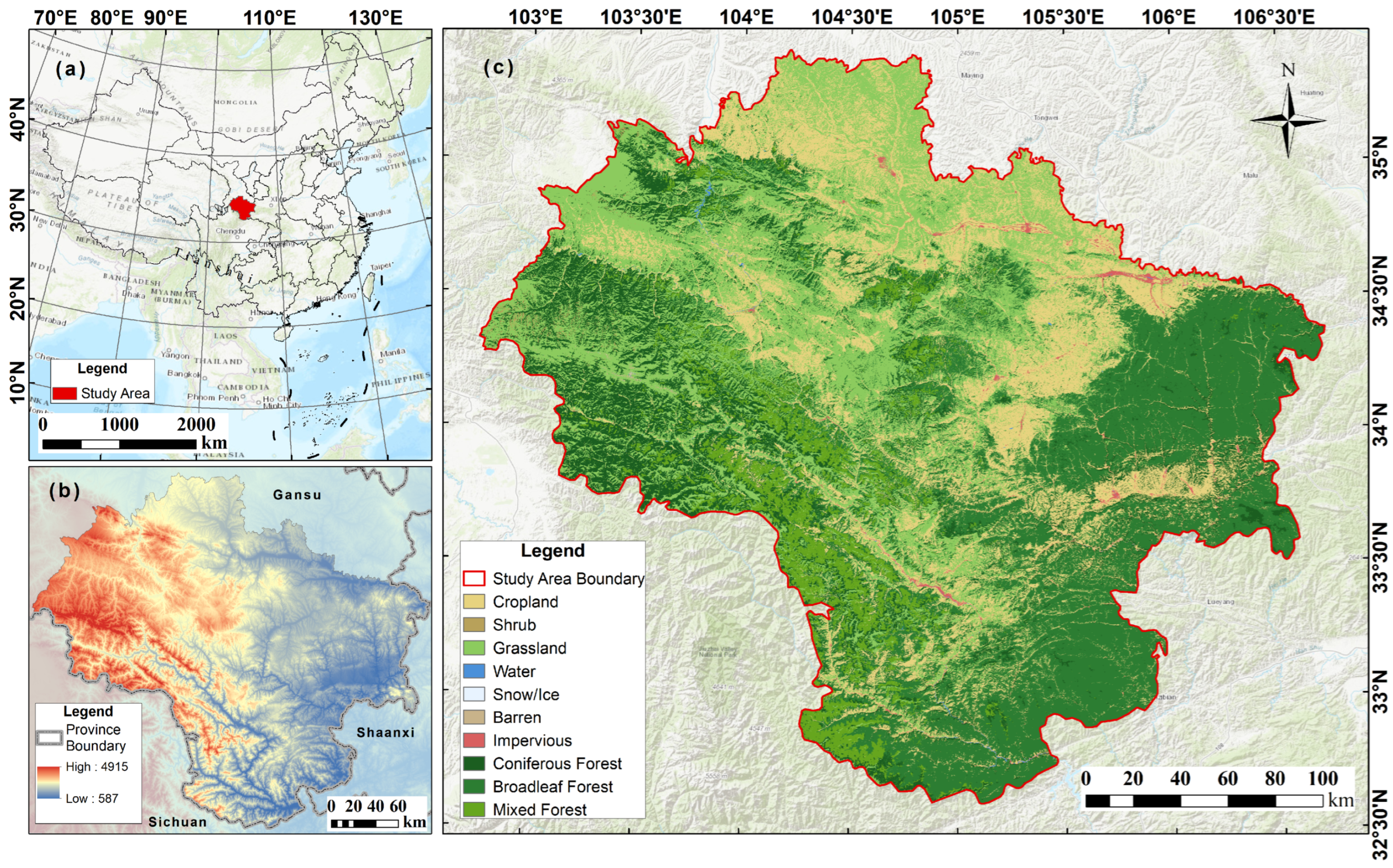
The study area follows the administrative boundaries of the West Qinling region in China and covers approximately 62,000 km2 in the southern area of Gansu Province. It forms a transitional zone between the Tibetan Plateau and the Loess Plateau and is characterized by complex terrain and strong environmental gradients. Based on boundary-clipped DEM statistics, elevation ranges from 587 to 4915 m. The climate is highly heterogeneous, transitioning from warm-temperate humid conditions in the southeast to alpine sub-humid conditions in the northwest, with mean annual temperatures of 5–15 °C and an annual precipitation of 400–900 mm. These climatic and topographic gradients support diverse vegetation types and make the region well suited for studying forest carbon dynamics. The regional forest mosaic is dominated by coniferous, broadleaf, and mixed forests distributed along elevation-dependent transition belts: coniferous stands are more frequent in cooler high-altitude sectors, broadleaf stands are concentrated in mid-elevation valleys and humid slopes, and mixed forests occupy transitional belts between these endmembers. This heterogeneity is also reflected at county scale. Counties such as Wenxian, Diebu, Wudu, Kangxian, and Maiji combine a comparatively large forest extent with strong recent net gains, while lower-gain counties tend to be more fragmented, drier, or more constrained by topography and human land use. We used the annual China Land Cover Dataset (CLCD) [10], specifically the 1985–2025 release accessed via Zenodo [11], to reconstruct land use trajectories for 2000–2025 at 30 m resolution. To capture forest heterogeneity, auxiliary remote sensing features were compiled for 2025, including spectral indices (Normalized Difference Vegetation Index [NDVI], Wetness [WET], and Normalized Difference Built-Up and Soil Index [NDBSI]), Land Surface Temperature (LST), and topographic variables derived from a Digital Elevation Model (DEM; elevation, slope, and aspect). Figure 1 summarizes the regional setting, topographic background, and baseline land use and vegetation context.

2.2. Remote Sensing Feature Engineering and Preprocessing

To construct the predictor space for forest subtype mapping, we used the Google Earth Engine (GEE) cloud computing platform to process multi-source satellite and terrain data for 2025. We used the Landsat 8/9 Collection 2 Tier 1 Surface Reflectance archive and applied the CFMask algorithm to remove clouds and cloud shadows before generating a median growing season mosaic (June–September). From this mosaic, we derived spectral and environmental predictors including NDVI, WET, NDBSI, LST, DEM, slope, and aspect. It should be noted that this predictor space is derived from 2025 imagery and therefore conditions the classifier on 2025 spectral–structural relationships. Transfer to earlier key years implicitly assumes that these subtype–feature relationships remained sufficiently stable over 2000–2025. In the present study, this should be regarded as a central structural limitation rather than as a minor caution because phenological variability, disturbance, succession, and interannual changes in canopy structure may all weaken the back transfer of a 2025-conditioned feature space.

2.3. Forest Subtype Classification, Validation, and Key-Year Transfer

We implemented a Random Forest (RF) classifier [15,16] in scikit-learn (v1.8.0) to distinguish forest subtypes within the 2025 CLCD forest mask. Candidate training samples were generated by aligning the 1:1,000,000 Chinese Vegetation Map with the 30 m feature raster and then screened using expected spectral and thermal ranges. As an additional quality control step, we conducted duplicate removal and class-wise robust outlier filtering before locking the final baseline sample set. These procedures were intended to reduce obvious label noise caused by mixed canopy signals or cartographic generalization during raster alignment, although they cannot fully eliminate scale mismatch between the source vegetation map and the Landsat analysis grid. Given that the 1:1,000,000 mapping minimum polygon corresponds to approximately 400 m × 400 m on the ground, the ∼13-fold linear scale difference relative to the 30 m Landsat grid introduces unavoidable boundary confusion, particularly within 1–2 pixels of polygon edges where topographic heterogeneity further complicates mixed canopy signals. Because independent field verification was not conducted, the contribution of this baseline label noise to overall classifier performance cannot be fully decoupled from other error sources. Consequently, the reported classification accuracies should be interpreted as inclusive of this baseline scale mismatch error. The final labeled reference dataset contained 2296 samples: 786 coniferous, 785 broadleaf, and 725 mixed.
To reduce bias from spatial autocorrelation, we used spatial block cross-validation [19]. Spatial groups were generated by quantile binning into a 6 × 6 lattice, yielding 36 quantile-defined spatial groups that were assigned to 5-fold GroupKFold. All pixels within a group were kept in the same fold to enforce geographic separation between training and validation subsets. The  6 × 6 lattice was selected as a balance between providing a sufficient number of spatial groups for stable 5-fold assignment (requiring at least 5 groups), maintaining a spatial block size that exceeds the typical spatial autocorrelation range reported for Landsat spectral features in similar forested mountain regions (typically <2–5 km), and ensuring that each fold contains a representative mixture of the three forest subtype classes. Finer lattices (e.g., 8 × 8 or 10 × 10 ) were not adopted because the resulting smaller blocks risked spatial leakage between training and validation folds given the 30 m pixel resolution. Hyperparameters were optimized by grid search over n_estimators  [ 150 , 300 , 500 ] , max_depth  [ N o n e , 20 , 30 ] , and min_samples_leaf  [ 1 , 2 , 4 ] . The selected model used 150 trees, no depth cap, and min_samples_leaf = 4. Performance was reported at three levels: overall accuracy, Cohen’s Kappa, and Macro-F1 for global discrimination; producer’s accuracy (recall), user’s accuracy (precision), and F1 for subtype-level reliability; and structural assessment of transferability for key-year application.
For temporally consistent subtype application, we implemented Scheme A by cautiously applying the trained RF classifier to six key years (2000, 2005, 2010, 2015, 2020, and 2025) and merging the predicted subtypes into each key-year CLCD map. Non-key years inherited the subtype map from the nearest preceding key year while preserving annual CLCD forest/non-forest updates. This strategy separates annual area dynamics from less frequent subtype structure updates and avoids endpoint-only subtype correction. Because harmonized historical reference labels and standardized spectral index stacks were not fully available for all key years in the current repository, the historical subtype allocation should be interpreted as a structural correction workflow rather than as a fully independent year-specific classification. This constitutes a strong structural approximation, because subtype persistence is assumed between key years, and real coniferous–broadleaf–mixed transitions occurring within those intervals are not directly reconstructed. Accordingly, the final temporal product is a hybrid series in which annual forest/non-forest extent is observed from the CLCD, whereas subtype composition between key years is structurally inherited rather than independently observed. Temporal subtype differences may therefore partly reflect a 2025-conditioned back-casting structure rather than the complete historical forest composition, and year-specific multitemporal feature stacks remain a priority for future work.
To partially diagnose temporal transfer under the current data archive, we additionally reconstructed a 2020 feature stack (NDVI, WET, NDBSI, LST, DEM, slope, and aspect) from the year-specific RSEI inputs and evaluated the 2025-trained RF model on a persistent-forest reference subset defined by pixels that remained forest in both the 2020 and 2025 CLCD masks. This diagnostic preserves spatial block separation and quantifies cross-year feature transfer degradation on a held-out subset, but it does not replace a full historical ground-truth validation because the reference labels are still anchored to the current baseline sample archive.

2.4. Carbon Accounting Model

Carbon stock estimation was adapted from the InVEST Carbon Storage and Sequestration model [22,23]. Total carbon stock for a given year ( C t ) was calculated by aggregating the carbon stored across four fundamental pools across all land use classes:
C t = i = 1 n A i , t × ( C a b o v e , i + C b e l o w , i + C s o i l , i + C d e a d , i )
where A i , t is the area (ha) of land use class i in year t. The terms C a b o v e , i , C b e l o w , i , C s o i l , i , and  C d e a d , i represent the carbon densities (Mg C ha−1) of the aboveground biomass, belowground biomass, soil organic carbon, and dead organic matter, respectively. Carbon density parameters were localized based on the regional literature and field survey syntheses for the West Qinling and adjacent regions [31,32,33,34]. A strict code-mapping algorithm ensured that all spatial pixels were accurately matched to their corresponding localized carbon parameters. These parameters are static over time and spatially uniform within each land use or subtype class; the model therefore attributes carbon change to land use or subtype transitions rather than to intra-class variation driven by stand age, density, management, or post-disturbance succession.

2.5. Uncertainty Analysis and Spatial Diagnostics

To address uncertainty in static carbon density parameters [24,25,26], we constructed three bounded parameter sensitivity scenarios by scaling the carbon densities of all forest-related classes (classes 2, 21, 22, and 23). The baseline scenario used the standard localized parameters (scaling factor 1.0), whereas the conservative (Low) and aggressive (High) scenarios applied scaling factors of 0.9 ( 10 % ) and 1.1 ( + 10 % ), respectively. These scenarios were designed as a targeted sensitivity test for forest-related pool parameters rather than as a complete uncertainty envelope for all land use classes and carbon pools. They are therefore informative regarding bounded forest pool sensitivity, but they do not capture the full uncertainty associated with forest mask error, non-forest pool parameters, temporal transfer, or broader structural assumptions in the accounting framework.
Spatial diagnostics were performed by calculating pixel-wise carbon density changes ( Δ C = C 2025 C 2000 ). We extracted absolute-magnitude hotspots (the top 10% of pixels experiencing the greatest absolute change) to visualize areas of intense ecological shift. Furthermore, county-level net changes were aggregated, and a transition contribution matrix was computed to trace the specific land use shifts associated with the regional carbon flux.
To propagate classification uncertainty into the subtype-dependent carbon component, we conducted a block bootstrap Monte Carlo experiment (10,000 iterations). In each iteration, the spatial block confusion matrix was resampled by bootstrapping blocks from the 6 × 6 lattice, posterior true class probabilities were recalculated from the resampled matrix, and subtype labels were then resampled before conversion to carbon stock using the same pool table. We report the mean, coefficient of variation, and 95% interval for the 2025 forest subtype component. This module addresses stochastic subtype assignment uncertainty under spatial dependence assumptions but it does not include CLCD forest mask uncertainty, broader pool-specific parameter uncertainty, historical temporal transfer uncertainty beyond the supplementary 2020 diagnostic, or independent external validation. The reported interval should therefore be interpreted as a partial uncertainty estimate for one component of the workflow rather than as a complete error envelope for total carbon accounting.
For county-scale interpretation, we further overlaid the 2025 subtype raster with county polygons and propagated the same block bootstrap posterior to the top five counties in baseline net carbon gain. The deterministic county net gain table was adjusted only through the uncertain 2025 subtype-dependent component; therefore, these county intervals should be interpreted as a classification-only extension rather than as a full county-level uncertainty budget. They are intended to support cautious comparison among leading counties, not to imply complete ranking certainty under all sources of model and data uncertainty.

2.6. Statistical Analysis

Temporal trends in total carbon stock (million Mg C) from 2000 to 2025 were analyzed using ordinary least squares (OLS) regression and the Hamed–Rao modified Mann–Kendall (MK) trend test [35]. OLS was used to estimate the linear slope, R 2 , and the 95% confidence interval for descriptive reference. Diagnostic tests included the Shapiro–Wilk test for residual normality, the Breusch–Pagan test for heteroscedasticity, and the Durbin–Watson test for autocorrelation. Because the OLS residuals exhibited severe positive autocorrelation (Durbin–Watson = 0.49), OLS-derived inferential statistics are not reliable for formal significance testing in this series. The Hamed–Rao modification corrects MK variance under serial dependence and therefore provides a more conservative significance estimate for autocorrelated annual carbon stock data. Sen’s slope was used as a robust estimate of the annual rate of change. All analyses were implemented in Python 3.13.12 using scipy (v1.17.1), statsmodels (v0.14.6), and pymannkendall (v1.4.3). AI-assisted coding features embedded in Trae IDE were used to support limited parts of the Python scripting and figure generation workflow during data processing and visualization. These tools were used only to assist code drafting and refinement; all code logic, parameter settings, analytical outputs, figures, and scientific interpretations were checked and validated by the authors, who take full responsibility for the final content.

2.7. Dual-Response GeoDetector Design with ERA5-Land Forcing

To explicitly separate factor associations with carbon state distribution from factor associations with carbon change dynamics, we implemented a dual-response GeoDetector framework with two response branches: (A) key-year carbon density stock distributions (2000, 2005, 2010, 2015, 2020, and 2025) and (B) carbon density change from 2000 to 2025. Terrain predictors included elevation, slope, aspect, relief, and incision depth. Climate predictors were derived from ERA5-Land monthly aggregates (ECMWF/ERA5_LAND/MONTHLY_AGGR) and included annual mean temperature (T2M), annual precipitation sum (P), annual downward shortwave radiation sum (SRAD), annual mean wind speed (WS), and annual mean relative humidity (RH, computed from 2 m temperature and dew point temperature).
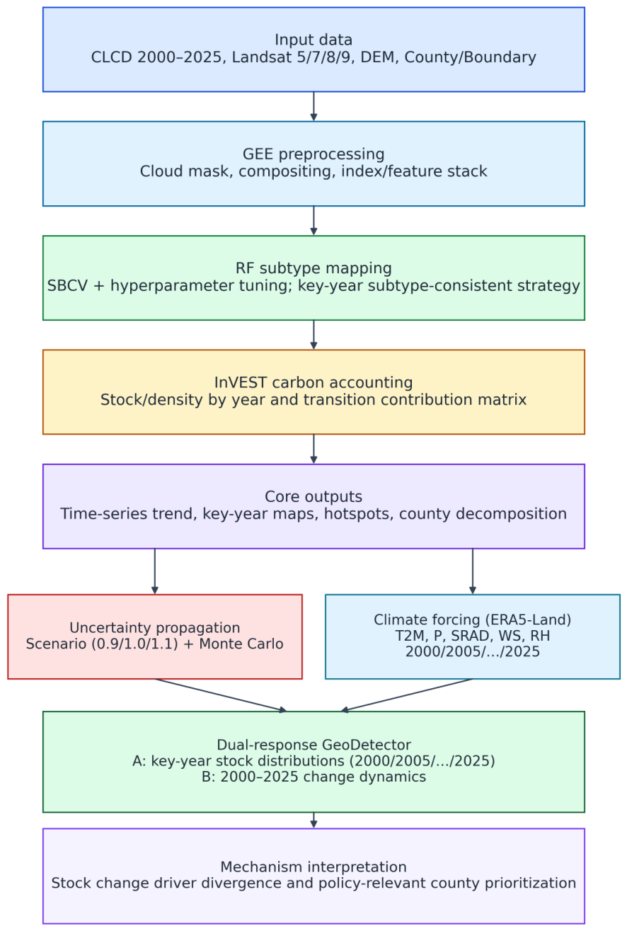
All predictor rasters were resampled and aligned to the response grid before sampling. For branch A, factor and interaction detectors were run independently for each key year using the year-matched stock raster and ERA5-Land climate composite. Branch B used the 2000–2025 stock difference raster. Factor discretization used quantile stratification ( k = 6 ). We computed factor detector q statistics, interaction detector q statistics with interaction-type classification, and permutation-based significance tests. To maintain computational comparability across branches and years, we used the same sampling cap ( n = 20,000 ), random seed, and permutation settings. The overall workflow is summarized in Figure 2.

2.8. Feature Definitions

The Normalized Difference Vegetation Index (NDVI), a fundamental proxy for photosynthetic activity and canopy density, was calculated as follows:
N D V I = ρ N I R ρ R e d ρ N I R + ρ R e d
where ρ N I R and ρ R e d represent the near-infrared and red band surface reflectances, respectively. To capture canopy moisture and stand structural complexity, we computed the Tasseled Cap Wetness (WET) index, which is highly sensitive to the water content of soil and vegetation. The Normalized Difference Built-Up and Soil Index (NDBSI) was integrated to contrast forested areas with bare earth and built environments, enhancing the separability of sparse forest stands.
Land Surface Temperature (LST) was derived from Landsat Thermal Infrared Sensor (TIRS) bands at their native thermal resolution and then harmonized to the 30 m analysis grid for multifeature stacking. We treated LST as an auxiliary discriminating feature rather than as a standalone subtype predictor. Topographic variables, specifically, elevation, slope, and aspect, were extracted from the NASA SRTM Digital Elevation Model (DEM) at 30 m resolution. In mountain environments, these variables strongly influence microclimate, solar radiation, and soil moisture and therefore help to explain the spatial distribution of forest subtypes.

3. Results

3.1. Performance of the Forest Subtype Model

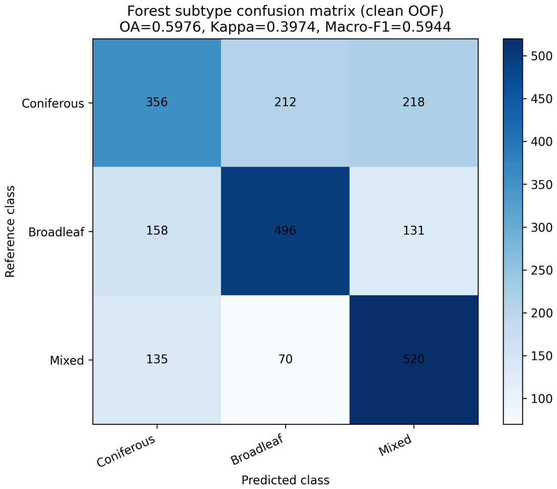
The spatially cross-validated Random Forest model achieved moderate performance in distinguishing forest subtypes across mountain terrain. Under strict spatial block validation, the model yielded an overall accuracy of 59.76%, a Cohen’s Kappa of 0.3974, and a Macro-F1 of 0.5944. According to the interpretation framework of Landis and Koch, this Kappa value indicates fair agreement rather than high-confidence discrimination. The confusion matrix shows substantial confusion among subtype pairs, especially between coniferous and mixed forests and between broadleaf and mixed forests, which is consistent with the spectral overlap in 30 m optical imagery. The low-cost enhancement test produced consistently lower SBCV metrics than the baseline setting, confirming that incremental sample filtering and balancing did not improve performance within the current feature space. This result supports our decision to retain the baseline RF configuration and prioritize transparent uncertainty propagation over further hyperparameter micro-tuning. On the persistent-forest subset used for the supplementary temporal transfer diagnostic ( n = 2124 ), the spatially held-out 2025 out-of-fold benchmark yielded OA = 56.17%, Kappa = 0.3402, and Macro-F1 = 0.5571, whereas transfer of the same 2025-trained model to the 2020 year-specific feature stack decreased performance to OA = 46.85%, Kappa = 0.2019, and Macro-F1 = 0.4654. The resulting declines ( Δ OA = 9.32 percentage points; Δ Kappa = 0.1383 ; Δ Macro-F1 = 0.0917 ) do not constitute a full historical validation, but they do quantify a non-trivial degradation in cross-year transfer under the current archive.
The confusion matrix used for Table 1 is 356 212 218 158 496 131 135 70 520 (rows: reference classes; columns: predicted classes). The largest directional confusion occurs between coniferous and broadleaf-adjacent mixed signals, indicating spectral overlap and mixed canopy boundaries in complex terrain. Although the diagonal remains visually prominent, the 924 off-diagonal errors among 2296 validation samples are sufficient to limit overall accuracy to 59.76% under spatial block validation. The corresponding confusion matrix visualization is shown in Figure 3.

3.2. Baseline Carbon Dynamics and Spatial Hotspots

Under the annual baseline workflow, the West Qinling region exhibited a positive net carbon change signal over the 25-year study period. Total carbon stock increased from 876.40 million Mg C in 2000 to 954.45 million Mg C in 2025, corresponding to a net gain of 78.05 million Mg C, or 8.91% relative to 2000. Mean regional carbon density increased accordingly from 141.35 to 153.94 Mg C ha−1.
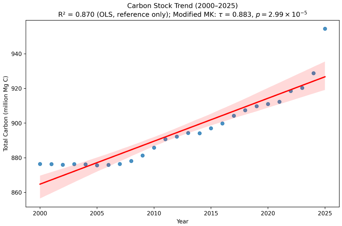
Figure 4 presents the annual time series of total carbon stock from 2000 to 2025 together with the fitted OLS trend and 95% confidence interval for visual reference. The trajectory indicates a persistent regional net increase pattern over 2000–2025, with no reversal in sink direction at the aggregate scale. However, apparent slope changes after 2010 should not be over-interpreted because the annual series is a hybrid product: forest/non-forest extent is updated annually, whereas subtype structure is refreshed only at key years. Because mean carbon density is a linear transformation of total stock under a fixed regional area, we report density values in the text and tables rather than plotting a redundant second curve.
Figure 4 shows a sustained positive trajectory in total carbon stock. OLS regression yielded a descriptive slope of 2.48 million Mg C year−1 ( R 2 = 0.870 ; 95% CI: 2.08–2.88); however, because the OLS residuals were non-normal and severely autocorrelated (Shapiro–Wilk p < 0.001 ; Durbin–Watson = 0.49), these OLS-derived inferential statistics are presented for reference only and are not used for formal trend inference. To obtain a statistically valid trend assessment under serial dependence, we applied the Hamed–Rao modified MK test, which confirmed a significant monotonic increase (Kendall’s τ = 0.883, modified p = 2.99 × 10 5 ; Sen’s slope = 2.41 million Mg C year−1). Within the present framework, this supports the interpretation of regional net accumulation at the aggregate scale over 2000–2025.
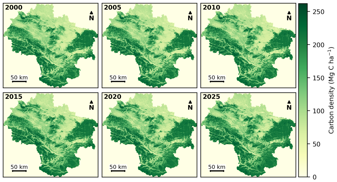
As a structural sensitivity check, the key-year spatial montage (Figure 5) shows that high-carbon-density zones remain concentrated in mountainous forest cores, while progressive infilling occurs along transition belts and foothill ecotones. Because these key-year maps are generated under the Scheme A inheritance workflow rather than by fully independent annual subtype reconstruction, this pattern should be interpreted as structurally smoothed evidence of persistent core accumulation rather than as direct observation of year-to-year subtype turnover. Within that boundary, the persistence of high-density nuclei combined with peripheral expansion is more consistent with a broad “core persistence + edge infilling” pattern than with random redistribution.
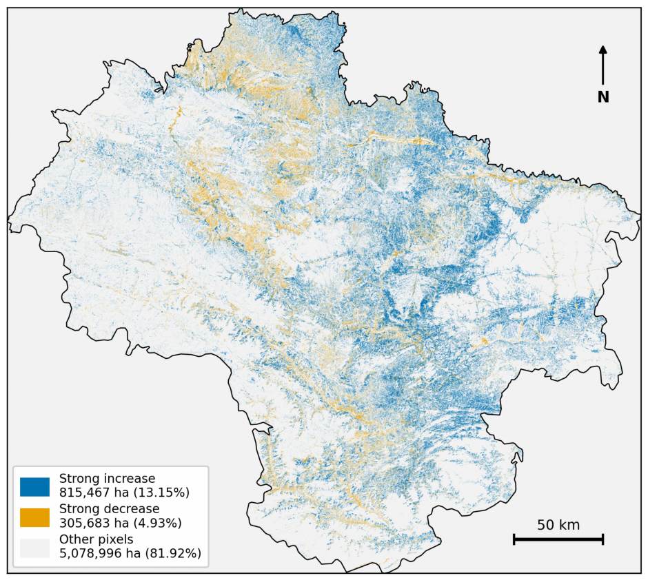
Figure 6 maps the absolute-magnitude hotspots (top 10% of change) and shows that intense carbon dynamics were overwhelmingly dominated by accumulation rather than decline. Under the annual baseline workflow, the absolute-magnitude threshold retained 769,032.54 ha of strong-increase hotspots and no strong-decrease hotspots, indicating pronounced asymmetry in regional change intensity under the current threshold definition.

3.3. Transition Pathways Associated with Carbon Accumulation Under Scheme A

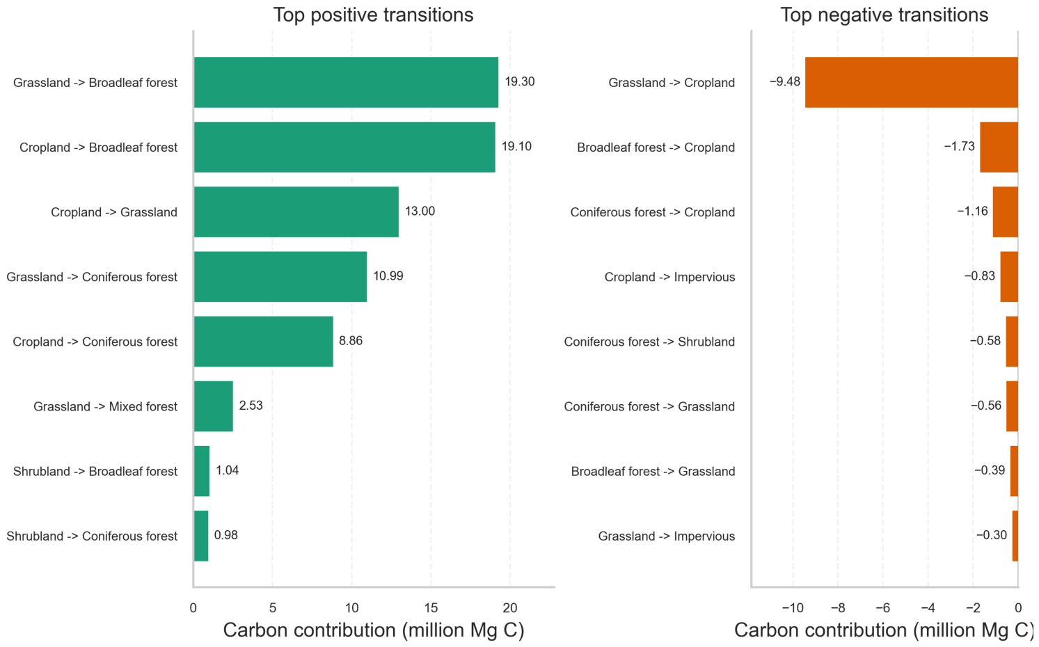
In the Scheme A structural sensitivity analysis, transition decomposition no longer contains major generic-forest recoding pathways. Instead, the largest positive contributions are associated with ecological conversion to broadleaf and coniferous classes: grassland to broadleaf (4 → 22, 19.30 million Mg C), cropland to broadleaf (1 → 22, 19.10 million Mg C), grassland to coniferous (4 → 21, 10.99 million Mg C), and cropland to coniferous (1 → 21, 8.86 million Mg C). This pattern suggests that the sink signal is more closely associated with subtype-resolved land cover transitions than with endpoint-only class relabeling. These pathways should nevertheless be interpreted as structurally inferred allocations under Scheme A rather than as direct observations of year-by-year ecological succession. For clarity, Figure 7 presents the leading positive and negative transitions in ranked form.

3.4. Dual-Response GeoDetector Results Under ERA5-Land Climate Forcing

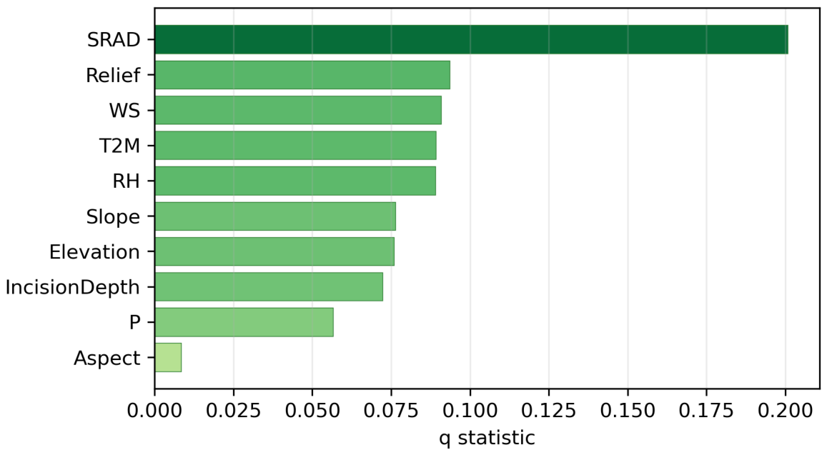
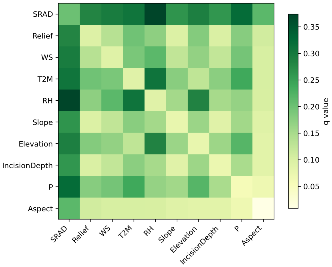
The dual-response analysis reveals a clear contrast between the factor associations for carbon stock and those for carbon change. In the key-year stock branch (2000/2005/2010/2015/2020/2025), SRAD consistently showed the highest single-factor q values (q range: 0.128036–0.202104), and SRAD × RH consistently showed the highest interaction q values (q range: 0.309168–0.369741). This cross-year consistency indicates a persistent association between radiative–hydrothermal coupling and stock heterogeneity under Scheme A.
For the 2025 carbon stock distribution specifically, SRAD showed the highest single-factor q value (q = 0.200792), followed by relief (q = 0.09358), WS (q = 0.090935), and T2M (q = 0.089268). The highest interaction q value was observed for SRAD × RH (q = 0.37391), suggesting a stronger combined spatial association than that of either factor alone. Figure 8 summarizes the single-factor q statistics for the 2025 stock branch, and Table 2 summarizes the highest-q factor and interaction across the six key years.
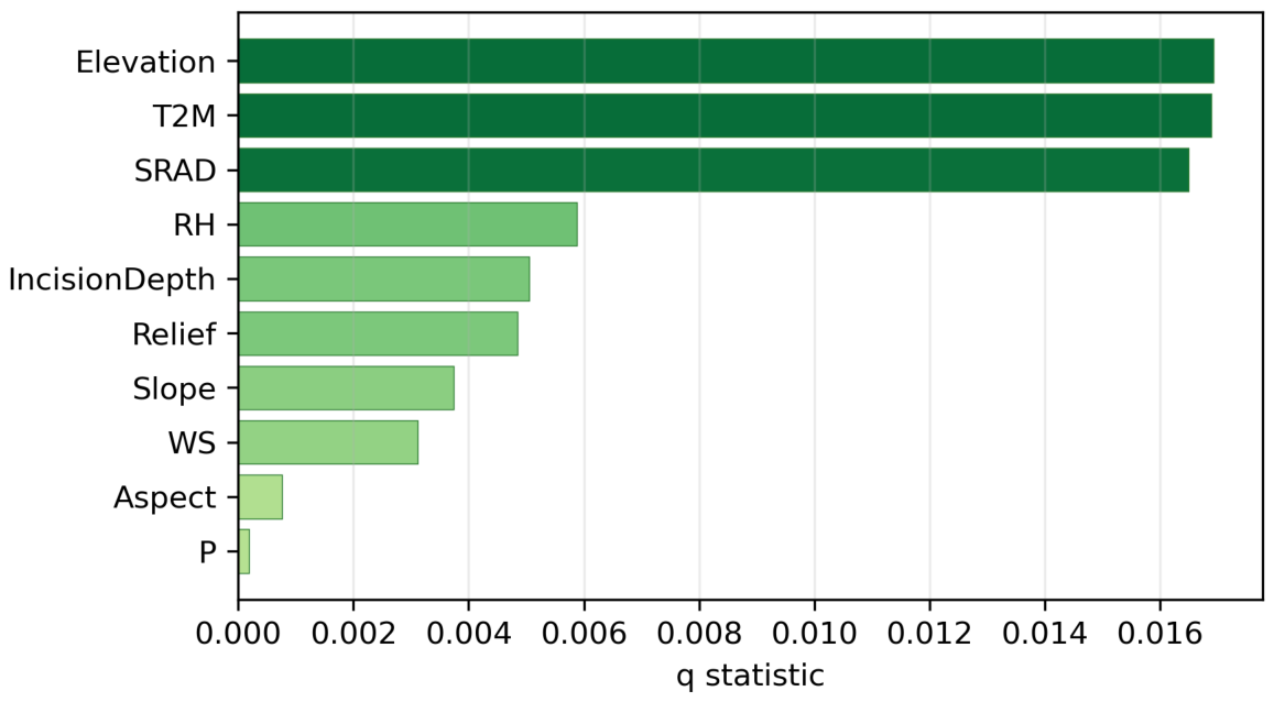
For carbon density change over 2000–2025, elevation showed the highest single-factor q value (q = 0.016929; permutation p = 0.025 ), closely followed by T2M (q = 0.016885) and SRAD (q = 0.01649). The highest interaction q value was observed for T2M × P (q = 0.030928). Because these q values are small, we interpret them as weak but detectable spatial associations rather than strong explanatory signals. Figure 9 summarizes the single-factor q statistics for the change branch. This state–change contrast suggests that long-term sink redistribution is only modestly associated with terrain baseline and climate coupling, whereas contemporary stock concentration shows stronger organization by energy–moisture structure. It also indicates that change dynamics are likely influenced by restoration history, land use transitions, and other management processes that are only partially represented by the static environmental predictors used in the GeoDetector framework. The 2025 interaction heatmap (Figure 10) further shows that interaction q values are systematically higher than single-factor q values, indicating non-additive spatial associations within the sampled predictor set.

3.5. Scenario Uncertainty and County-Level Robustness

The parameter sensitivity analysis provided a bounded interval for the carbon estimates (Table 3). Total carbon stock in 2025 ranged from 887.07 million Mg C in the Low scenario to 1021.84 million Mg C in the High scenario. These bounded scenarios were used as a targeted sensitivity analysis of forest-related carbon density parameters rather than as a complete uncertainty envelope for all pools and land use classes. Despite this parameter uncertainty, the net change from 2000 to 2025 remained positive in all scenarios, ranging from 66.47 to 89.64 million Mg C.
As a structural sensitivity analysis, Scheme A key-year subtype-consistent accounting yielded a net gain of 60.19 million Mg C. Compared with endpoint-only subtype fusion, this more conservative estimate indicates that part of the previously reported gain reflected temporal structural inconsistency rather than ecological change alone.
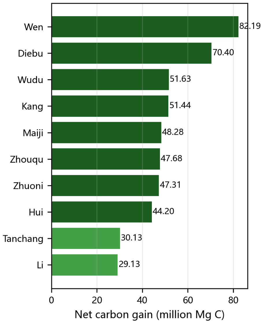
At the county management scale, the ranking of net carbon gain was comparatively stable under the bounded parameter perturbations tested here. Across the Low, Baseline, and High scenarios, the same five administrative units consistently ranked highest: Wenxian County, Diebu County, Wudu District, Kangxian County, and Maiji District. The values displayed in Figure 11 are taken directly from the same baseline county table summarized in Appendix C Table A3. They represent county-level net forest carbon gain under the baseline workflow and should not be interpreted as methodologically identical to the regional total net carbon change reported for the full accounting series or the Scheme A structural sensitivity total.
To propagate classification uncertainty into the forest subtype carbon component, we conducted a Monte Carlo simulation (10,000 iterations) using a block bootstrap uncertainty model. In each iteration, the spatial block confusion matrix was resampled by bootstrapping spatial blocks (derived from the 6 × 6 lattice), then used to generate posterior true class probabilities for resampling subtype labels. The resulting 95% interval for the 2025 forest subtype carbon component was 676.07–689.05 million Mg C (mean 682.36 million Mg C; CV = 0.478%), indicating that classification uncertainty produces a non-negligible range at regional scale under spatial dependence assumptions. The relatively narrow interval reflects regional aggregation: although pixel-level subtype confusion is moderate, a substantial portion of local error cancels when the forest subtype component is summed across the full study area. This interval should be interpreted as conditional on the current subtype allocation structure and posterior assumptions; it does not represent a full regional uncertainty budget and does not include the CLCD forest mask error, broader pool parameter uncertainty, or other spatially correlated errors beyond the current forest-related classes. When this classification-only extension was propagated to the top five counties in baseline net carbon gain, all five counties retained positive net gains and Wenxian and Diebu remained clearly the first and second contributors. The adjusted 95% intervals were 83.49–85.01 million Mg C for Wenxian and 66.63–68.35 million Mg C for Diebu, while Wudu (53.08–54.30 million Mg C) and Kangxian (53.40–54.73 million Mg C) showed overlapping intervals, indicating that their relative ordering should not be over-interpreted under classification uncertainty alone. These county intervals remain conditional because they do not include CLCD mask uncertainty, full parameter uncertainty, or temporal transfer error.

4. Discussion

4.1. Reliability of Carbon Estimates and Comparison with Previous Qinling Studies

The integration of forest subtypes materially altered the regional carbon baseline within the current accounting framework. By disaggregating the generic forest class into coniferous, broadleaf, and mixed forests, the model assigned higher biomass densities to the broadleaf and mixed stands that are common in parts of the West Qinling region. Consequently, if these subtypes were aggregated back into a single broader forest category, the magnitude of the observed carbon accumulation trend would likely be underestimated, as the generic parameters fail to capture the disproportionate contribution of high-density broadleaf expansion. This finding is broadly consistent with national-scale assessments [5,12], which show that ignoring forest composition can underestimate carbon stocks in structurally diverse mountain ecosystems. In addition, the use of spatial block cross-validation [19] reduces the risk of the overly optimistic accuracy estimates often reported in remote sensing classification studies and therefore provides a more defensible basis for downstream carbon accounting.
The moderate subtype classification performance (OA = 59.76%, Kappa = 0.3974) has different implications across spatial scales. At the pixel or stand scale, subtype confusion can translate directly into carbon density misallocation, especially where coniferous, broadleaf, and mixed forests intergrade along mountain ecotones. At the regional aggregation scale, however, a substantial portion of this error may be attenuated through spatial averaging. This behavior is consistent with the block bootstrap Monte Carlo interval for the 2025 forest subtype component (676.07–689.05 million Mg C), which remains comparatively narrow after regional aggregation even though local classification uncertainty is non-trivial. County-level aggregates may therefore be less sensitive than pixel-level subtype assignments, but local interpretation should still be treated cautiously in fragmented or transition-zone forests.
At the regional comparison level, the sink direction identified here is consistent with recent Qinling studies reporting net carbon accumulation under restoration and land cover optimization [27,28,29,30]. At the same time, those studies generally emphasize prediction, optimization, NPP trajectories, or broader Qinling–Daba regional totals, whereas the present study places stronger emphasis on subtype-resolved carbon accounting under spatial validation and explicit structural constraints. Differences in absolute magnitude are therefore expected not only because spatial scopes differ (the West Qinling versus broader Qinling–Daba domains), but also because temporal continuity, subtype treatment, and uncertainty reporting are not equivalent across studies. Similar issues have been noted in other mountain regions of western China, where carbon estimates vary substantially depending on whether studies rely on generic land cover classes, historical land use reconstruction, or county-oriented management units [36,37,38]. Our contribution is therefore not intended to replace previous estimates directly, but to provide a structurally constrained, county-oriented accounting workflow in which temporal transfer assumptions and uncertainty components are reported explicitly.

4.2. Processes Associated with Regional Carbon Accumulation

The net carbon gain observed across all tested scenarios (66.47 to 89.64 million Mg C) is compatible with the regional restoration trajectory reported for northwestern China. Within the structural constraints of the current workflow, the transition matrix assigns comparatively large contributions to pathways such as grassland to broadleaf forest, which is broadly compatible with the restoration-oriented land cover change reported under the Grain for Green Program and related forest protection initiatives [6,7,14,31,39]. This directional consistency is helpful for interpreting the aggregate sink signal, but it should not be taken to mean that the subtype-resolved pathway magnitudes are externally validated. These pathways should instead be read as structurally inferred allocations of carbon change contribution rather than as direct annual observations of ecological succession. The county-level pattern likewise suggests that counties with extensive mountainous terrain and sustained restoration activity (e.g., Wenxian County, Diebu County) may contribute relatively strongly at the regional scale, but finer ranking differences remain conditional on the current uncertainty scope.
The dual-response GeoDetector results provide a complementary description of spatial association patterns. Carbon stock distribution shows comparatively stable associations with SRAD across the six key years, and SRAD × RH repeatedly yields the highest interaction q values. By contrast, the carbon change branch shows much smaller q values, with elevation, T2M, and T2M × P ranking highest within a weaker association set. This contrast suggests that static stock patterning is more clearly aligned with persistent topo-climatic gradients than carbon change dynamics are under the tested covariates. Accordingly, the GeoDetector outputs are retained as descriptive spatial associations rather than as primary explanatory evidence for the observed carbon change patterns.

4.3. Uncertainties, Limitations, and Future Directions

Although the scenario analysis shows that the direction of carbon change is robust, magnitude-based policy targets must still account for parameter uncertainty [24,25,40]. Scheme A addresses the core temporal inconsistency by applying forest subtype mapping to six key years (2000, 2005, 2010, 2015, 2020, and 2025). In this study, we retain the annual baseline workflow as the primary accounting series because it preserves full annual CLCD continuity, whereas Scheme A is used as a structural sensitivity reference that reveals how subtype inheritance assumptions alter long-term magnitudes. Even after adding the 2020 transfer diagnostic, however, historical temporal validation remains incomplete. The persistent-forest diagnostic shows a clear degradation from the held-out 2025 benchmark (OA = 56.17%) to the 2020 transfer test (OA = 46.85%), indicating that cross-year feature transfer introduces a non-trivial performance penalty under the current archive. Scheme A should therefore be interpreted as a structurally consistent sensitivity reference with comparatively conservative magnitude estimates rather than as a fully reconstructed annual truth estimate. Future work should replace proxy historical transfer with year-specific multitemporal index stacks, dedicated historical reference sets, and dynamic age-dependent carbon densities [3,41,42]. Coupling climate scenarios with land use simulation models (e.g., PLUS or CA-Markov) would further support predictive carbon risk assessment under alternative socioeconomic pathways.
Four additional limitations warrant emphasis: First, independent external validation against GEDI, airborne or terrestrial LiDAR, or NFI observations was not completed in this revision. Absolute stock levels should therefore be interpreted more cautiously than relative spatial patterns [43]. Second, the InVEST-style pool table uses static SOC and dead organic matter parameters and therefore does not represent gradual post-restoration soil carbon accumulation or depletion over decadal timescales. Third, the present uncertainty analysis remains incomplete and should be read component by component. The bounded parameter scenarios quantify uncertainty in total carbon under forest-related pool perturbation. The subtype Monte Carlo interval quantifies classification uncertainty only for the 2025 forest subtype component, and the county-level extension propagates that same source only into the top-five-county net gain table. Scheme A represents structural sensitivity in subtype allocation. Because these outputs address different uncertainty sources, they cannot be combined into a single regional interval without hierarchical spatiotemporal error propagation. CLCD forest mask uncertainty, broader pool-specific parameter variation, temporal transfer bias beyond the current 2020 diagnostic, and fully hierarchical spatiotemporal error propagation have not yet been modeled and may still widen local and county-level uncertainty ranges [21,44]. Fourth, the temporal trend analysis is affected by serial autocorrelation. The Durbin–Watson statistic of 0.49 for OLS residuals indicates severe positive autocorrelation, which invalidates OLS-based significance testing. We therefore relied on the Hamed–Rao modified MK test for formal trend inference. Future analyses could further evaluate autoregressive or state-space time series models for annual carbon stock series.

4.4. Policy Implications

Under the annual baseline workflow, the region showed aggregate net carbon gain from 2000 to 2025, with a net gain of 78.05 million Mg C. From an implementation perspective, county-level prioritization remains informative but conditional: Wenxian County, Diebu County, Wudu District, Kangxian County, and Maiji District remain the leading contributors under all tested parameter scenarios. The classification-only county extension further indicates that Wenxian and Diebu remain comparatively well separated from the remaining counties, whereas Wudu and Kangxian should be treated as a partially overlapping second tier rather than as decisively ordered priorities. These counties therefore warrant closer attention in ecological compensation, forest quality management, and long-term disturbance monitoring, but any finer ranking should remain conditional on the current uncertainty scope. Scheme A provides a more conservative estimate under key-year subtype-consistent accounting and indicates that structural assumptions about subtype allocation can materially affect long-term magnitude estimates. For conservative benchmarking, the Scheme A net gain of 60.19 million Mg C may be used as a reference value only if it is interpreted as a structural sensitivity result rather than as a full uncertainty bound, replacement primary estimate, or policy-ready estimate. At the provincial scale, the results provide a spatially explicit reference for regional carbon accounting discussion and monitoring design. They should nevertheless be applied with caution because county-level prioritization remains conditional on the current validation, forest mask, parameter, and temporal transfer assumptions [36,37,38].

5. Conclusions

This study presents a reproducible workflow for estimating forest carbon dynamics in the West Qinling Mountains by integrating CLCD land use data with spatially validated machine learning subtype classification and InVEST-based accounting. Under the annual baseline workflow, total carbon stock increased from 876.40 million Mg C in 2000 to 954.45 million Mg C in 2025, yielding a net gain of 78.05 million Mg C. Within the current modeling framework, this aggregate accounting series is consistent with regional net accumulation, but subtype-specific historical inference remains constrained by moderate classification performance and incomplete temporal transfer validation. A supplementary 2020 transfer diagnostic on a persistent-forest subset showed measurable degradation relative to the held-out 2025 benchmark, reinforcing that temporal transfer remains a substantive limitation. Scheme A key-year subtype-consistent accounting yielded a more conservative net gain of 60.19 million Mg C and is therefore retained as a structural sensitivity reference rather than a replacement primary estimate. The annual series should not be interpreted as a record of independently reconstructed year-specific subtype transitions because historical subtype structure was transferred through key-year updating rather than rebuilt from year-specific spectral stacks. The reported uncertainty intervals are conditional rather than exhaustive: they do not yet include CLCD forest mask error, full pool parameter uncertainty, or a hierarchical spatiotemporal error budget, and the county-level extension remains limited to classification-induced uncertainty in the 2025 subtype-dependent component. Future work should therefore extend both the temporal feature stacks and the uncertainty framework before the results are used for stronger decision or accounting claims.

Author Contributions

Conceptualization, L.N.; methodology, Q.B. and L.N.; software, Q.B.; validation, L.N. and B.L.; formal analysis, Q.B.; investigation, Q.B.; resources, L.N.; data curation, B.L.; writing—original draft preparation, Q.B.; writing—review and editing, L.N. and B.L.; visualization, Q.B.; supervision, L.N.; project administration, L.N.; funding acquisition, L.N. All authors have read and agreed to the published version of the manuscript.

Funding

This research was funded by the Special Project for Scientific Research Innovation Team Building of Tianshui Normal University (Grant No. TDJ2023-04) and the Youth Doctoral Support Project of Gansu Provincial Department of Education (Grant No. 2023QB-008).

Institutional Review Board Statement

Not applicable.

Informed Consent Statement

Not applicable.

Data Availability Statement

A Zenodo deposition has been created for this study (prereserved DOI: https://doi.org/10.5281/zenodo.19363219, accessed on 24 July 2026). Upon publication of the deposition, the processed outputs used in this manuscript will be openly available there, including the Results/Carbon and Results/ForestSubtype collections. The CLCD source used in this study is openly available via Zenodo (https://doi.org/10.5281/zenodo.18180184, accessed on 24 July 2026; [11]) and is documented in [10]. Landsat source products used in this study are publicly accessible via USGS. GEDI products are publicly accessible via NASA Earthdata and are noted here as potential future validation resources, but they were not used for independent validation in the present analysis. Additional intermediate files can be provided by the corresponding author upon reasonable request.

Acknowledgments

The authors acknowledge the project team for data preparation and workflow testing support. The authors also acknowledge the use of AI-assisted coding features embedded in Trae IDE to support limited parts of Python scripting and visualization script refinement, as well as Grammarly for Windows (v1.2.280.1927) for English language checking. These tools were used only to support implementation and language polishing; study design, parameter setting, result verification, interpretation, and final manuscript approval were performed by the authors.

Conflicts of Interest

The authors declare no conflicts of interest.

Abbreviations

CLCDChina Land Cover Dataset
DEMDigital Elevation Model
LSTLand Surface Temperature
NDBSINormalized Difference Built-Up and Soil Index
NDVINormalized Difference Vegetation Index
RFRandom Forest

Appendix A. Detailed Carbon Density Parameters

To ensure the reproducibility of the InVEST carbon accounting model, the localized carbon density parameters for all land use classes are provided in Table A1. These parameters were synthesized from the regional literature and field survey reports specifically targeting the West Qinling Mountains and adjacent ecosystems.
Table A1. Localized carbon density parameters for all land use and forest subtype classes used in the baseline scenario. Carbon pools include aboveground ( C a b o v e ), belowground ( C b e l o w ), soil organic carbon ( C s o i l ), and dead organic matter ( C d e a d ). All values are in Mg C ha−1. Forest (Generic, class 2) is retained only as a fallback parameter class and is not present in Scheme A key-year subtype-constrained LULC maps.
Land Use Class (Code) C above C below C soil C dead Total
Cropland (1)15.204.3085.601.20106.30
Forest (Generic) (2)48.5012.30110.204.50175.50
Coniferous Forest (21)42.3010.50105.403.80162.00
Broadleaf Forest (22)55.6014.80120.505.20196.10
Mixed Forest (23)50.1012.60115.304.60182.60
Shrubland (3)18.408.2095.302.10124.00
Grassland (4)6.5015.4088.700.80111.40
Water (5)0.000.0015.200.0015.20
Snow/Ice (6)0.000.000.000.000.00
Barren (7)0.500.2010.500.0011.20
Impervious (8)2.100.5045.300.0047.90
Wetland (9)8.5012.30135.601.50157.90

Appendix B. Hyperparameter Optimization Grid

The Random Forest classifier was optimized using a spatial block cross-validation strategy. Table A2 details the hyperparameter combinations evaluated during the grid search and their corresponding cross-validation performance metrics.
Table A2. Hyperparameter grid search results for the Random Forest forest subtype classifier sorted by Mean CV Score (overall accuracy). The best-performing model parameters are highlighted in bold.
n_estimatorsmax_depthmin_samples_leafMean CV Score
150None40.5977
200None40.5965
100None40.5952
1502040.5948
2002040.5941
1002040.5935
150None20.5912
200None20.5908
100None20.5895
50None40.5882
1501040.5750
2001040.5745
1001040.5732
502040.5721
150None10.5650
200None10.5645

Appendix C. County-Level Net Forest Carbon Gain

The spatial distribution of net forest carbon gain is highly heterogeneous across the administrative units of the West Qinling region. Table A3 summarizes county-level net forest carbon gain and associated forest area dynamics from 2000 to 2025 under the baseline workflow. Counties are ranked by net gain in descending order. These county totals support administrative comparison under the baseline workflow, but they should not be directly compared with the region-wide net carbon change values in the main text because the scopes and aggregation definitions are not identical.
Table A3. County-level net forest carbon gain and forest area dynamics under the baseline workflow (2000–2025). Net gain is reported in million Mg C. The county totals are provided for administrative comparison within Appendix C and are not directly equivalent to the region-wide net carbon change values reported in the main text.
County/DistrictNet Gain (Million Mg C)Increase Area (ha)Decrease Area (ha)Mean Change (Mg C ha−1)
Wenxian County82.19399,165.3920,395.35162.84
Diebu County70.40301,330.534685.13148.96
Wudu District51.63288,605.7928,065.60110.93
Kangxian County51.44264,888.993653.19172.72
Maiji District48.28250,571.8810,071.81137.85
Zhouqu County47.68221,604.759602.28157.45
Zhuoni County47.31215,206.565688.4592.12
Hui County44.20217,066.501947.51162.37
Tanchang County30.13159,004.4422,789.7190.76
Li County29.13193,360.8622,264.1168.33
Liangdang County26.97128,757.96641.88188.42
Chengxian County21.55110,056.323540.06128.20
Qinzhou District15.61110,693.078633.8865.89
Xihe County13.9892,684.798744.6775.37
Zhang County13.4077,676.4817,817.0361.85
Minxian County13.2884,846.6935,328.6937.12
Lintan County9.0749,817.702852.4665.08
Wushan County8.0762,736.9313,249.8040.49
Weiyuan County5.4245,912.3327,203.8526.39
Gangu County3.2649,461.219889.9220.62
Lianhuashan Scenic Forest Reserve1.768144.73236.43158.11
Longxi County1.2752,957.1724,726.425.26
Regional total636.01

Appendix D. Detailed Land Use Transition Contributions

To trace the structurally inferred land use shifts associated with the regional carbon signal, the carbon stock changes were decomposed into specific land use transition pathways under Scheme A key-year subtype-consistent maps. Table A4 lists representative transition pathways contributing to the regional carbon dynamics between 2000 and 2025. These pathways should be interpreted as outputs of the adopted key-year inheritance framework rather than as direct annual observations of ecological succession.
Table A4. Representative land use transition pathways and their contribution to total regional carbon stock change (2000–2025) under Scheme A. Positive values indicate carbon sequestration; negative values indicate carbon emission. Contributions are reported in million Mg C. The listed pathways are structurally inferred under key-year inheritance and should not be read as independently observed annual transition histories.
From Class (2000)To Class (2025)Carbon Contribution (Million Mg C)
GrasslandBroadleaf Forest19.298
CroplandBroadleaf Forest19.101
CroplandGrassland12.998
GrasslandConiferous Forest10.986
CroplandConiferous Forest8.861
GrasslandMixed Forest2.532
ShrublandBroadleaf Forest1.039
ShrublandConiferous Forest0.981
CroplandMixed Forest0.328
BarrenGrassland0.077
ShrublandMixed Forest0.071
WaterGrassland0.046
ShrublandGrassland0.029
GrasslandImpervious 0.298
Broadleaf ForestGrassland 0.388
Coniferous ForestGrassland 0.557
CroplandWater 0.118
Broadleaf ForestShrubland 0.219
Mixed ForestCropland 0.263

Appendix E. Supplementary County-Level Ecological Interpretation

The regional carbon dynamics are an aggregation of localized ecological responses to topography, climate, and policy interventions. County-level interpretation is provided to support practical implementation of carbon management actions.
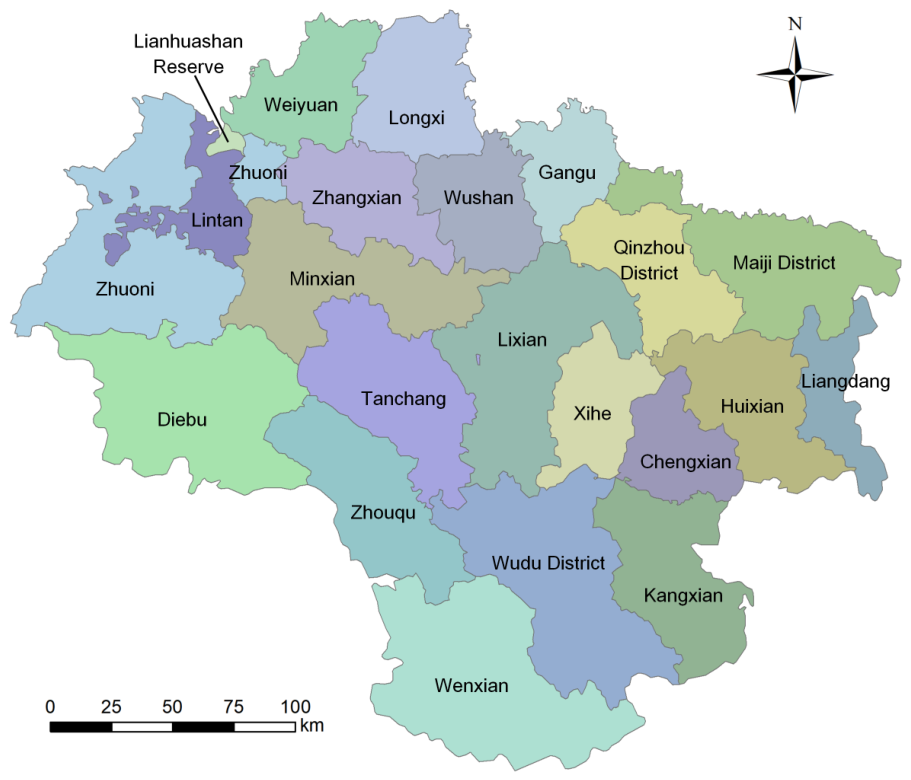
Figure A1. County-level administrative reference map of the West Qinling study area used to locate the county descriptions in Appendix E. Boundaries and labels are provided for rapid geographic lookup.
Forests 17 00867 g0a1

Appendix E.1. Leading Contributors

Wenxian County and Diebu County jointly represent the strongest carbon accumulation core in the region. Their net gains are supported by a large forest extent, low-intensity disturbance regimes in key mountain zones, and continued maturation of broadleaf and mixed stands. Wudu District, Kangxian County, and Maiji District form the second tier of high-contribution counties, where policy-driven restoration and terrain-conditioned regeneration interact. Wenxian County combines high baseline forest coverage with favorable hydrothermal conditions. A high proportion of broadleaf and mixed forests in medium-elevation belts supports a relatively high carbon density and sustained annual increment. Diebu County contributes a similar scale of net gain through extensive conifer-dominated mountain stands and long-term logging restrictions that reduced disturbance frequency. In Wudu District, the main mechanisms include not only forest growth but also the structural conversion of slope cropland under restoration policy; this conversion has coupled effects on erosion reduction and biomass accumulation. Kangxian County and Maiji District show a mixed pathway where planted forests and natural recovery coexist. Their results suggest that stand quality and age structure are now as important as area expansion for further carbon gains.

Appendix E.2. Middle-Tier Counties

Zhouqu County, Chengxian County, Minxian County, and Qinzhou District show consistent but moderate gains. In these counties, carbon trajectories reflect mixed land use contexts: slope cropland retirement, patchy urban expansion, and varying stand maturity. The measured gain suggests restoration momentum is present but constrained by local development pressure and a fragmented landscape structure. Zhouqu County presents a typical case where ecological restoration is strongly coupled with geological risk management. Reforestation and shrub recovery on unstable slopes generate carbon co-benefits while improving slope stability, but long-term permanence remains sensitive to extreme rainfall events. Chengxian County and Minxian County are characterized by fragmented forest patches embedded in agricultural matrices, where edge effects and local disturbance intensity limit average carbon density growth. Qinzhou District shows a dual trend: the urban core expands impervious surfaces, while surrounding mountain sectors continue to recover forest cover. This duality explains why county totals remain positive despite strong local source areas.

Appendix E.3. Lower-Gain Counties and Management Implications

Tanchang County, Hui County, Liangdang County, and Xihe County show smaller absolute gains, partly due to having smaller county areas or drier conditions in local sectors. For these areas, management priority should focus on improving forest quality and connectivity rather than simply expanding area, including enrichment planting in suitable microsites and better mitigation of local degradation pressures. In lower-gain counties, the marginal return of additional area-based afforestation can be limited by water availability, slope constraints, and fragmented ownership patterns. Tanchang and Hui Counties benefit from targeted connectivity enhancement that links existing forest patches and reduces ecological isolation. Liangdang County has comparatively high per-hectare stock in mature stands, implying that strict protection of high-quality remnants can yield better long-term outcomes than broad but low-survival planting campaigns. Xihe County requires drought-adapted strategies emphasizing native shrub–tree mosaics, soil–water conservation engineering, and grazing pressure management. Across these counties, a quality-oriented approach is likely to produce more stable carbon outcomes than purely area-driven targets.

Appendix F. Supplementary Topographic Constraint Analysis

Appendix F.1. Elevation Gradient

Elevation strongly structures moisture and thermal regimes, shaping a non-linear carbon density pattern. Lower elevations are dominated by cropland and settlement systems with relatively low carbon density. Mid-elevation belts support the most productive broadleaf and mixed forests and therefore host the strongest carbon sinks. At higher elevations, low temperature and shallow soils limit biomass accumulation, shifting vegetation toward sparse coniferous forest, shrubland, and grassland. This elevational response implies that climate warming may have asymmetric effects across zones. In middle-elevation belts, warmer conditions could initially increase growing season length and productivity, but moisture deficits or disturbance events may offset gains. In upper belts, treeline movement may increase woody cover in selected microsites, yet gains are constrained by substrate depth, freeze–thaw stress, and wind exposure. Therefore, elevation-based zoning is required when interpreting regional carbon trends: apparent regional gains can mask opposite local responses across altitudinal strata. Future monitoring should report carbon trajectories by elevation bands to improve attribution and management targeting.

Appendix F.2. Slope and Aspect Controls

Slope is a practical determinant of restoration feasibility and land use conversion. The largest positive changes are concentrated on moderate-to-steep slopes where cropland retirement under restoration policy was strongest. Aspect further modifies the microclimate: north-facing slopes generally maintain higher soil moisture and support denser canopy development than south-facing slopes in drier subregions. These terrain associations suggest that future restoration planning should be terrain-adaptive, species-matched, and explicitly microclimate-aware. From a planning perspective, slope and aspect should be integrated into a priority matrix for species selection and silvicultural treatment. Moderate north-facing slopes are suitable for mixed-forest enhancement and structural diversification, while steeper south-facing slopes should prioritize drought-tolerant native assemblages and soil conservation measures. In highly dissected terrain, road access and management logistics also shape feasibility, meaning the biophysically optimal area is not always operationally optimal. A practical compromise is to prioritize areas with both high sequestration potential and manageable intervention cost, then apply adaptive management based on survival and growth feedback.

Appendix G. Supplementary Uncertainty Propagation Notes

Parameter perturbation and classification propagation analyses jointly indicate that uncertainty sources operate at different scales. Parameter scenarios (±10%) dominate variation in total regional magnitude, while confusion matrix propagation under the current posterior structure adds relatively small aggregate variation for the forest subtype component. This pattern does not eliminate classification uncertainty at the local scale; rather, it indicates that large-area aggregation attenuates pixel-level misclassification effects. Future work should couple full time series subtype mapping with spatially explicit posterior probabilities to better capture local uncertainty heterogeneity. Methodologically, this also highlights a separation between structural uncertainty and stochastic uncertainty. Structural uncertainty now mainly arises from key-year transfer assumptions in Scheme A, especially the use of temporally fixed ancillary spectral index features. Stochastic uncertainty arises from parameter and classification variability conditioned on that structure. The present uncertainty intervals should therefore be interpreted as conditional on the Scheme A structure. For future revisions, an integrated hierarchical framework that jointly estimates annual subtype trajectories, class-conditional carbon densities, and spatially explicit uncertainty surfaces would provide more policy-relevant confidence bounds, especially for county-level compensation and project verification workflows.
Figure A2. Monte Carlo distribution (10,000 iterations) of the 2025 forest subtype carbon component after confusion matrix-based classification uncertainty propagation.
Forests 17 00867 g0a2

Appendix H. Supplementary County Notes for Management Practice

Appendix H.1. Wenxian County

Wenxian County remains the most prominent carbon-contributing unit in this study. Its large net gain is associated with contiguous mountain forests, a high share of broadleaf and mixed forest structure, and relatively limited fragmentation in core sectors. From a management standpoint, the main priority is permanence: conserving mature stands while strengthening fire risk prevention and pest monitoring. Any significant disturbance in this county would have disproportionate regional consequences.

Appendix H.2. Diebu County

Diebu County contributes substantial gains in all scenarios. Conifer-dominated belts at higher elevation are the dominant sink component. Because growth rates are sensitive to moisture deficit and temperature extremes, adaptation-oriented silviculture and disturbance surveillance are critical. Maintaining stand heterogeneity can reduce systemic vulnerability.

Appendix H.3. Wudu District

Wudu District shows strong gains linked to slope land restoration and ongoing stand development. The county is also a representative case of restoration–development interaction. Continued gains depend on balancing agricultural production demands with ecological red-line protection and slope stability objectives.

Appendix H.4. Kangxian County and Maiji District

Kangxian County and Maiji District jointly form a major secondary sink cluster. Their trajectories indicate that quality improvement of existing forests can be as important as area increase. Enrichment planting, thinning optimization, and mixed-stand enhancement are practical pathways for long-term stability.

Appendix H.5. Zhouqu and Cheng Counties

These counties demonstrate moderate but stable accumulation. Gains are spatially uneven, with high-sensitivity zones in steep and geologically active terrain. Carbon management should therefore be co-designed with disaster risk reduction and soil conservation programs.

Appendix H.6. Minxian County and Qinzhou District

In Minxian County, high-elevation constraints limit rapid biomass increase, implying that persistence and gradual quality improvement are more realistic objectives than short-term sequestration targets. In Qinzhou District, urban expansion pressure coexists with mountain restoration, requiring a dual-zone strategy that protects peri-urban ecological corridors.

Appendix H.7. Tanchang, Hui, Liangdang, and Xihe Counties

These counties show smaller absolute gains but remain important for regional continuity of sink function. Strategies should prioritize connectivity restoration, drought-resilient species composition, and localized degradation mitigation. In particular, Xihe requires water-aware restoration plans and strict mitigation of chronic disturbance pressures.

Appendix H.8. Cross-County Implementation Priorities

Three operational priorities emerge consistently across counties: first, maintaining the top-contributor counties as stability anchors for regional carbon budgets; second, improving stand quality and connectivity in middle- and lower-gain counties rather than targeting only area expansion; third, integrating terrain constraints and microclimate into species and treatment selection to maximize survival and permanence. These priorities align with the uncertainty findings and support risk-informed ecological investment.

Appendix H.9. Monitoring Framework for Verification and Adaptive Management

To operationalize county-level strategies, a standardized monitoring framework is required. At minimum, annual monitoring should include land cover transitions, subtype composition shifts, stand condition indicators, and disturbance inventories. Satellite-based indicators can provide wall-to-wall annual updates, while field plots should be used for calibration and bias correction in representative ecological zones. A two-tier protocol is recommended: Tier 1 for annual rapid screening and Tier 2 for targeted in-depth verification in priority counties. Tier 1 can rely on harmonized remote sensing products and automated quality checks. Tier 2 should focus on plot-based biomass validation, stand age structure, and disturbance diagnostics where model uncertainty or policy relevance is high. This design enables both cost efficiency and scientific credibility in long-term carbon accounting.

Appendix H.10. Implications for Carbon Finance and Ecological Compensation

The heterogeneity observed in county contributions implies that a uniform compensation rule is suboptimal. Performance-linked ecological compensation can improve both fairness and effectiveness. Counties with high and stable sequestration should receive long-term conservation incentives tied to permanence safeguards, while counties with lower baseline gains should be supported through capacity-building and restoration quality programs. For carbon finance integration, project design should prioritize additionality demonstration, disturbance risk buffering, and transparent MRV workflows. The uncertainty intervals reported in this study provide a practical foundation for risk-adjusted crediting and conservative baseline setting. Importantly, carbon finance should not incentivize short-term area expansion at the expense of ecological resilience. A resilience-first design that combines sequestration targets with quality and permanence indicators is more consistent with long-horizon climate objectives.

Appendix I. Supplementary Reproducibility and Quality Control Protocol

Appendix I.1. Workflow Reproducibility Architecture

The complete workflow follows a deterministic stage-based architecture designed to minimize hidden analyst decisions. Stage 1 ingests annual CLCD rasters and validates projection consistency, class code completeness, and nodata behavior. Stage 2 executes feature engineering for subtype classification and applies strict sample filtering rules to avoid mixed-pixel contamination in steep terrain. Stage 3 trains and validates the classifier under spatial block cross-validation. Stage 4 performs carbon accounting using harmonized pool tables and year-specific override logic. Stage 5 executes sensitivity and uncertainty modules, including parameter perturbation and confusion matrix propagation. Stage 6 generates publication graphics and summary tables. Each stage writes structured outputs to fixed directories and avoids in-memory-only results, enabling direct auditability.

Appendix I.2. Input Integrity Checks

Before model execution, all raster and tabular inputs are subjected to integrity checks. Raster checks include CRS equivalence, pixel size conformity, bounded class code ranges, and nodata propagation tests under map algebra operations. Tabular checks include unique class identifiers, non-negative carbon densities, and explicit four-pool completeness for all active classes. The implementation enforces failure-fast behavior: if any mandatory check fails, processing stops and reports the exact source file and variable. This prevents silent propagation of malformed inputs and substantially improves reliability for multi-stage geospatial pipelines.

Appendix I.3. Spatial Validation Controls

Spatial leakage is handled by assigning folds at block level rather than random pixel level. This design prevents geographically adjacent pixels from being simultaneously used for training and validation. Fold balance is monitored to avoid severe class imbalance in any single fold. In addition to global metrics, class-level precision and recall diagnostics are tracked to detect directional bias in subtype assignment. Confusion analysis is interpreted ecologically rather than purely numerically, acknowledging that structurally similar canopy types may remain difficult to separate at 30 m resolution.

Appendix I.4. Carbon Accounting Safeguards

Carbon accounting is performed under explicit rule constraints to avoid structural inconsistencies. The 2025 subtype map is only used in 2025 by design, while historical years retain generic forest coding. A fallback pool table is used to preserve historical comparability and prevent class-missing collapse in legacy years. All units are standardized to Mg C and hectare-based density representations before aggregation. Intermediate products include per-class area, per-class carbon density, per-year totals, and county-level summaries, so each aggregate value can be traced back to explicit components.

Appendix I.5. Uncertainty and Sensitivity Reporting Standards

The uncertainty framework distinguishes between parameter uncertainty and classification uncertainty. Parameter uncertainty is assessed through deterministic perturbation scenarios with clearly stated scaling factors and targeted class sets. Classification uncertainty is propagated through Monte Carlo simulation using posterior class probabilities derived from the confusion matrix. Both components are reported with intervals, central tendency, and coefficient of variation where appropriate. This dual framing avoids overconfidence in point estimates and aligns output with decision-making contexts that require risk-aware interpretation.

Appendix I.6. Figure and Table Production Standards

All manuscript-critical figures were generated from scripts, not manual editing tools, to ensure one-command reproducibility. For publication requirements, each new figure was exported in both vector and high-resolution raster formats. Axis labels, units, and legend hierarchy follow a uniform style guide. Numeric formatting is harmonized across figures and tables to reduce interpretation error. Script-based generation also allows rapid regeneration if source data are updated during revision cycles, which is essential in peer-review response workflows.
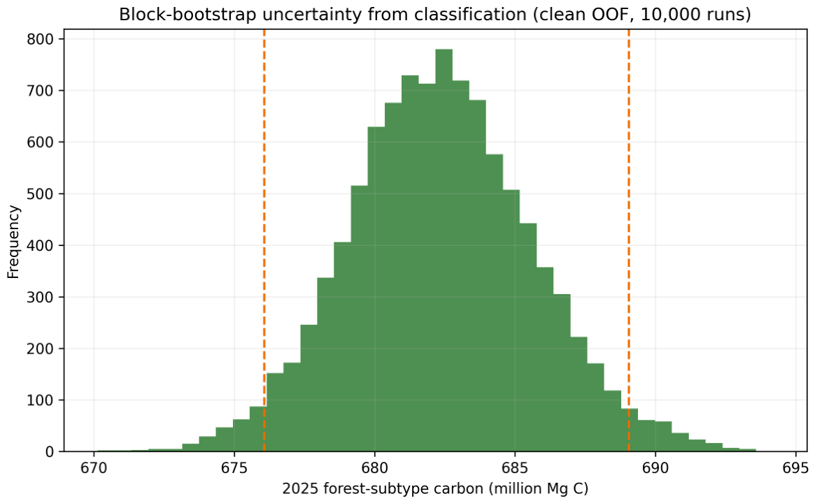
Appendix I.7. Independent Re-Run Strategy

To verify reproducibility, the pipeline can be re-run from raw inputs in a clean environment. The recommended strategy is to recreate the Python environment from dependency files, execute stage scripts sequentially, and compare checksum-level identities for key output tables. For non-deterministic modules, fixed random seeds are enforced and output tolerances are documented. This design supports independent verification by collaborators and reviewers and reduces dependency on a single workstation configuration.

Appendix I.8. Limitations of the Current Reproducibility Scope

Although the workflow is script-driven, two constraints remain: First, temporal consistency is currently implemented at six key years rather than the full annual sequence, and historical ancillary spectral features are proxied by a harmonized 2025 stack. Second, external quality services such as commercial grammar checking and institutional plagiarism systems are outside the current runtime environment. These constraints are documented explicitly in the revision package and are scheduled for closure before final submission packaging.

Appendix I.9. Forward Research Agenda for Submission-Ready Expansion

To support next-round submission quality, three extensions are prioritized: First, temporal subtype reconstruction should be expanded from a single-year endpoint to a full annual sequence, enabling direct ecological change attribution without structural inconsistency. Second, county-level policy evaluation should be linked to explicit intervention timelines, allowing causal interpretation of restoration effects rather than descriptive association. Third, uncertainty should be reported as spatially explicit surfaces, not only regional intervals, so management agencies can target monitoring resources to high-uncertainty zones. Implementing these extensions will strengthen both scientific inference and policy usability while preserving the reproducible architecture developed in this study.

Appendix J. Supplementary Annual Carbon Time Series Table

Table A5. Annual total carbon stock (million Mg C) and mean carbon density (Mg C ha−1) in the West Qinling region (2000–2025).
YearTotal Carbon (Million Mg C)Mean Carbon Density (Mg C ha−1)
2000876.40141.351
2001876.35141.344
2002875.95141.278
2003876.32141.338
2004876.18141.315
2005875.63141.227
2006875.88141.268
2007876.42141.355
2008878.08141.622
2009881.30142.142
2010885.81142.868
2011890.68143.654
2012892.19143.898
2013894.28144.235
2014894.12144.209
2015897.04144.680
2016899.82145.129
2017904.20145.836
2018907.40146.351
2019909.72146.726
2020910.97146.927
2021912.33147.147
2022918.56148.151
2023920.31148.433
2024928.79149.802
2025954.45153.940

References

  1. Houghton, R.A. The role of forests in the global carbon cycle. Forests 2020, 11, 681. [Google Scholar] [CrossRef] [Scilit]
  2. Pan, Y.; Birdsey, R.A.; Fang, J.; Houghton, R.; Kauppi, P.E.; Kurz, W.A.; Phillips, O.L.; Shvidenko, A.; Lewis, S.L.; Canadell, J.G.; et al. A large and persistent carbon sink in the world’s forests. Science 2011, 333, 988–993. [Google Scholar] [CrossRef] [Scilit] [PubMed]
  3. Harris, N.L.; Gibbs, D.A.; Baccini, A.; Birdsey, R.A.; de Bruin, S.; Farina, M.; Fatoyinbo, L.; Hansen, M.C.; Herold, M.; Houghton, R.A.; et al. Global maps of twenty-first century forest carbon fluxes. Nat. Clim. Chang. 2021, 11, 234–240. [Google Scholar] [CrossRef] [Scilit]
  4. Piao, S.; Fang, J.; Ciais, P.; Peylin, P.; Huang, Y.; Sitch, S.; Wang, T. The carbon balance of terrestrial ecosystems in China. Nature 2009, 458, 1009–1013. [Google Scholar] [CrossRef] [Scilit] [PubMed]
  5. Tang, X.; Zhao, X.; Bai, Y.; Tang, Z.; Wang, W.; Zhao, Y.; Wan, H.; Xie, Z.; Shi, X.; Wu, B.; et al. Carbon pools in China’s terrestrial ecosystems: New estimates based on an intensive field survey. Proc. Natl. Acad. Sci. USA 2018, 115, 4021–4026. [Google Scholar] [CrossRef] [Scilit] [PubMed]
  6. Liu, J.; Li, S.; Ouyang, Z.; Tam, C.; Chen, X. Ecological and socioeconomic effects of China’s policies for ecosystem services. Proc. Natl. Acad. Sci. USA 2008, 105, 9477–9482. [Google Scholar] [CrossRef] [Scilit] [PubMed]
  7. Viña, A.; McConnell, W.J.; Yang, H.; Xu, Z.; Liu, J. Effects of conservation policy on China’s forest recovery. Sci. Adv. 2016, 2, e1500965. [Google Scholar] [CrossRef] [Scilit] [PubMed]
  8. Pan, Y.; Tian, Y.; Wu, Y.; Fu, M. A comprehensive approach for the spatial optimization of the biodiversity conservation network in the Qinling Mountains, China. Landsc. Ecol. 2025, 40, 11. [Google Scholar] [CrossRef] [Scilit]
  9. Cai, Y.; Zhu, P.; Li, X.; Liu, X.; Chen, Y.; Shen, Q.; Xu, X.; Zhang, H.; Nie, S.; Wang, C.; et al. Dynamics of China’s forest carbon storage: The first 30 m annual aboveground biomass mapping from 1985 to 2023. Earth Syst. Sci. Data 2025, 17, 6993–7018. [Google Scholar] [CrossRef] [Scilit]
  10. Yang, J.; Huang, X. The 30 m annual land cover dataset and its dynamics in China from 1990 to 2019. Earth Syst. Sci. Data 2021, 13, 3907–3925. [Google Scholar] [CrossRef] [Scilit]
  11. Yang, J.; Huang, X. The 30 m annual land cover datasets and its dynamics in China from 1985 to 2025. Zenodo 2026. [Google Scholar] [CrossRef]
  12. Zhang, H.; Li, P.; Liu, J. High-resolution mapping of forest carbon density using multi-source remote sensing data. Int. J. Appl. Earth Obs. Geoinf. 2022, 108, 102715. [Google Scholar] [CrossRef] [Scilit]
  13. He, M.; Chen, X.; Liu, Y. Forest subtype mapping using multi-temporal optical and SAR data: A case study in the Qinling Mountains. Remote Sens. 2021, 13, 700. [Google Scholar] [CrossRef] [Scilit]
  14. Wang, J.; Li, Y.; Chen, T. Dynamics of ecosystem carbon storage and their response to land use change in the upper Yellow River basin. Ecol. Indic. 2023, 146, 109825. [Google Scholar] [CrossRef] [Scilit]
  15. Breiman, L. Random forests. Mach. Learn. 2001, 45, 5–32. [Google Scholar] [CrossRef] [Scilit]
  16. Li, R.; Fang, P.; Xu, W.; Wang, L.; Ou, G.Z. Classifying forest types over a mountainous area in Southwest China with Landsat data composites and multiple environmental factors. Forests 2022, 13, 135. [Google Scholar] [CrossRef] [Scilit]
  17. Zhang, W.; Liu, X.; Xu, B.; Liu, J.; Li, H. Remote sensing classification and mapping of forest dominant tree species in the Three Gorges Reservoir area based on sample migration and machine learning. Remote Sens. 2024, 16, 2547. [Google Scholar] [CrossRef] [Scilit]
  18. Yuan, J.; Wu, Z.; Li, S.; Kang, P.; Zhu, S. Multi-feature-based identification of subtropical evergreen tree species using Gaofen-2 imagery and algorithm comparison. Forests 2023, 14, 292. [Google Scholar] [CrossRef] [Scilit]
  19. Roberts, D.R.; Bahn, V.; Ciuti, S.; Boyce, M.S.; Elith, J.; Guillera-Arroita, G.; Hauenstein, S.; Lahoz-Monfort, J.; Schröder, B.; Thuiller, W.; et al. Cross-validation strategies for data with space, time and/or phylogenetic structure. Ecography 2017, 40, 913–929. [Google Scholar] [CrossRef] [Scilit]
  20. Meyer, H.; Reudenbach, C.; Hengl, T.; Katurji, M.; Bendix, J. Improving performance of continuous predictions of soil properties in spatial modeling. Environ. Model. Softw. 2018, 109, 211–221. [Google Scholar] [CrossRef] [Scilit]
  21. Ploton, P.; Mortier, F.; Réjou-Méchain, M.; Barbier, N.; Picard, N.; Rossi, V.; Dormann, C.; Cornu, G.; Viennois, G.; Bayol, N.; et al. Spatial validation reveals poor predictive performance of large-scale ecological mapping models. Nat. Commun. 2020, 11, 4540. [Google Scholar] [CrossRef] [Scilit] [PubMed]
  22. Sharp, R.; Tallis, H.; Ricketts, T.; Guerry, A.; Wood, S.; Chaplin-Kramer, R.; Nelson, E.; Ennaanay, D.; Wolny, S.; Olwero, N.; et al. InVEST User Guide; Stanford University: Stanford, CA, USA; University of Minnesota: Minneapolis, MN, USA; The Nature Conservancy: Arlington, VA, USA; World Wildlife Fund: Washington, DC, USA, 2020. [Google Scholar]
  23. Tallis, H.; Ricketts, T.; Guerry, A.; Wood, S.; Sharp, R.; Nelson, E.; Ennaanay, D.; Wolny, S.; Olwero, N.; Vigerstol, K.; et al. InVEST 2.4.4 User’s Guide; Technical Report; The Natural Capital Project: Stanford, CA, USA, 2013. [Google Scholar]
  24. Lu, X.; Zhang, Y.; Lin, C. Evaluating the spatial uncertainty of InVEST carbon model with Monte Carlo simulation. Sci. Total Environ. 2018, 628, 845–854. [Google Scholar] [CrossRef] [Scilit] [PubMed]
  25. Hamel, P.; Bryant, B.P. Uncertainty assessment in ecosystem services analyses: Seven challenges and practical responses. Ecosyst. Serv. 2017, 24, 1–15. [Google Scholar] [CrossRef] [Scilit]
  26. Metsaranta, J.M.; Shaw, C.; Kurz, W.A.; Boisvenue, C.; Morken, S. Uncertainty of inventory-based estimates of the carbon dynamics of Canada’s managed forest (1990–2014). Can. J. For. Res. 2017, 47, 1082–1094. [Google Scholar] [CrossRef] [Scilit]
  27. Chen, W.; Li, X.; Wang, Z. Prediction and Evolution of Carbon Storage of Terrestrial Ecosystems in the Qinling Mountains North Slope Region, China. Land 2023, 12, 2063. [Google Scholar] [CrossRef] [Scilit]
  28. Bai, T.; Gong, E.; Zhou, N.; Zhao, T.; Bai, H.; Wang, J. Spatiotemporal Patterns and Driving Forces Analysis of Ecological Carbon Sink from 2001 to 2022 in Qinling–Daba Mountains, China. Environ. Sci. 2025, 46, 356–366. [Google Scholar] [CrossRef] [Scilit] [PubMed]
  29. Yuan, Y.; Huang, G.R.; Zhao, T.; Zhang, X.; Zheng, M. Spatio-temporal variations and climatic and human activity driving factor analysis of net primary productivity (2000–2022) in the Qinling Shaanxi section of China. J. Indian Soc. Remote Sens. 2025, 54, 737–753. [Google Scholar] [CrossRef] [Scilit]
  30. Xu, X.; Yan, S.; Peng, X. Carbon sequestration effects of the typical restored vegetation types in Eastern Qinling Mountains. Acta Bot.-Boreali Sin. 2025, 45, 115–124. [Google Scholar] [CrossRef]
  31. Zhao, Z.; Dong, Z.; Wang, X. Assessing the impacts of afforestation programs on carbon sequestration in the Loess Plateau. For. Ecol. Manag. 2022, 505, 119890. [Google Scholar] [CrossRef] [Scilit]
  32. Huang, H.; Liu, C.; Wang, X.; Zhou, X.; Gong, P. Integration of multi-resource remotely sensed data and allometric models for forest aboveground biomass estimation in China. Remote Sens. Environ. 2019, 228, 225–242. [Google Scholar] [CrossRef] [Scilit]
  33. Liu, J.; Yang, B.; Li, M.; Xu, D. Assessing forest-change-induced carbon storage dynamics by integrating GF-1 imagery and localized allometric growth equations in Jiangning District, Nanjing, Eastern China (2017–2020). Forests 2024, 15, 506. [Google Scholar] [CrossRef] [Scilit]
  34. Fang, J.; Chen, A.; Peng, C.; Zhao, S.; Ci, L. Changes in forest biomass carbon storage in China between 1949 and 1998. Science 2001, 292, 2320–2322. [Google Scholar] [CrossRef] [Scilit] [PubMed]
  35. Hamed, K.H.; Rao, A.R. A modified Mann–Kendall trend test for autocorrelated data. J. Hydrol. 1998, 204, 182–196. [Google Scholar] [CrossRef] [Scilit]
  36. Li, K.; Cao, J.; Adamowski, J.; Biswas, A.; Zhou, J. Assessing the effects of ecological engineering on spatiotemporal dynamics of carbon storage from 2000 to 2016 in the Loess Plateau area using the InVEST model: A case study in Huining County, China. Environ. Dev. 2021, 38, 100641. [Google Scholar] [CrossRef] [Scilit]
  37. An, Y.; Tan, X.; Ren, H.; Li, Y.; Zhou, Z. Historical changes and multi-scenario prediction of land use and terrestrial ecosystem carbon storage in China. Chin. Geogr. Sci. 2024, 34, 487–503. [Google Scholar] [CrossRef] [Scilit]
  38. Deng, S.; Zhang, M.; Wang, Y.; Hou, Y.; Yu, E. Assessing spatiotemporal variation of forest aboveground carbon sequestration coupling landscape models with remote sensing datasets in Western Sichuan, China. In Proceedings of the IGARSS 2024–2024 IEEE International Geoscience and Remote Sensing Symposium; IEEE: Piscataway, NJ, USA, 2024; pp. 1–4. [Google Scholar] [CrossRef] [Scilit]
  39. Zhang, X.; Wu, Q.; Chen, S.; He, W.; Jiang, J.; Wang, L. The Grain for Green Program boosted vegetation greening and carbon assimilation in the Loess Plateau from 2001 to 2019. SSRN Electron. J. 2024. [Google Scholar] [CrossRef] [Scilit]
  40. Piao, S.; He, Y.; Wang, X.; Chen, F. Estimation of China’s terrestrial ecosystem carbon sink: Methods, progress and prospects. Sci. China Earth Sci. 2022, 65, 641–651. [Google Scholar] [CrossRef] [Scilit]
  41. Huang, D.; Ding, X.; Wang, Y.; Peng, Z. Using PLUS-InVEST-OPGD model to explore spatiotemporal variation of ecosystem carbon storage and its drivers in Jinsha river basin, China. PeerJ 2025, 13, e19681. [Google Scholar] [CrossRef] [Scilit] [PubMed]
  42. Zhang, Z.; Zhang, Z.; Li, X.; Feng, Y. Mechanisms for carbon stock driving and scenario modeling in typical mountainous watersheds of northeastern China. Environ. Monit. Assess. 2024, 196, 891. [Google Scholar] [CrossRef] [Scilit] [PubMed]
  43. Dubayah, R.; Blair, J.B.; Goetz, S.; Fatoyinbo, L.; Hansen, M.; Healey, S.; Hofton, M.; Hurtt, G.; Kellner, J.; Luthcke, S.; et al. The Global Ecosystem Dynamics Investigation: High-resolution laser ranging of the Earth’s forests and topography. Sci. Remote Sens. 2020, 1, 100002. [Google Scholar] [CrossRef] [Scilit]
  44. Roxburgh, S.H.; Paul, K.I. Comprehensive propagation of errors for the prediction of woody biomass. Methods Ecol. Evol. 2024, 15, 2106–2124. [Google Scholar] [CrossRef] [Scilit]
Figure 1. Study area overview with three coordinated panels: (a) The national-scale location of the West Qinling study area in southern Gansu, adjacent to Shaanxi and Sichuan, with the study area outline highlighted for geographic context. (b) The elevation background derived from the boundary-clipped DEM showing an in-area altitudinal range of 587–4915 m and major topographic gradients across the mountain system. (c) The spatial pattern of baseline land use and vegetation classes within the study boundary, including cropland, shrub, grassland, water, snow/ice, barren land, impervious surfaces, and forest subtypes (coniferous, broadleaf, and mixed). A county-level administrative reference map with labels is provided in Appendix E for location lookup of county descriptions.
Forests 17 00867 g001
Figure 2. Technical roadmap of the integrated workflow, including Scheme A key-year subtype-consistent mapping, annual/key-year carbon accounting, and dual-response GeoDetector analysis.
Forests 17 00867 g002
Figure 3. Forest confusion matrix evaluated under spatial block cross-validation for the 2025 forest subtype classification.
Forests 17 00867 g003
Figure 4. Annual baseline workflow carbon stock dynamics (2000–2025). The fitted OLS trend and shaded 95% confidence interval are shown for visual reference only; formal trend inference is based on the Hamed–Rao modified Mann–Kendall test.
Forests 17 00867 g004
Figure 5. Spatial distribution of carbon density at six key years (2000, 2005, 2010, 2015, 2020, and 2025) under Scheme A subtype-consistent accounting. The subtype maps shown here are generated through key-year inheritance and structural transfer rather than through independent annual classifications for every year.
Forests 17 00867 g005
Figure 6. Absolute-magnitude hotspot map (top 10%) for carbon density change from 2000 to 2025 under the annual baseline workflow, highlighting the dominance of intense carbon accumulation over decline. The mapped change field follows the hybrid annual accounting series in which forest/non-forest extent is updated annually but subtype structure is not independently reconstructed for every year.
Forests 17 00867 g006
Figure 7. Ranked land use transition contributions to carbon change (2000–2025) under Scheme A, showing top positive and top negative pathways in million Mg C. These pathway rankings are derived from key-year inheritance and structural subtype transfer, not from independent annual transition mapping. Because subtype composition between key years is structurally inherited rather than independently observed, the transition pathways shown here should be interpreted as products of the key-year inheritance scheme rather than as directly observed annual succession events. This ranking-based display improves readability under highly skewed transition magnitudes.
Forests 17 00867 g007
Figure 8. Factor detector q statistics for the 2025 carbon stock distribution response under dual-response GeoDetector analysis.
Forests 17 00867 g008
Figure 9. Factor detector q statistics for the 2000–2025 carbon density change response under dual-response GeoDetector analysis.
Forests 17 00867 g009
Figure 10. Interaction detector heatmap for the 2025 carbon stock distribution response, with stronger greens indicating larger interaction q values.
Forests 17 00867 g010
Figure 11. Top 10 counties by net forest carbon gain from 2000 to 2025 under the annual baseline workflow. These county values are directly linked to Appendix C Table A3 and are not numerically equivalent to the regional total net carbon change reported for the full study area.
Forests 17 00867 g011
Table 1. Subtype classification performance summary under spatial block cross-validation.
SubtypeProducer’s Accuracy (%)User’s Accuracy (%)F1
Coniferous45.2954.850.4962
Broadleaf63.1863.750.6347
Mixed71.7259.840.6524
OverallAccuracy = 59.76%Kappa = 0.3974Macro-F1 = 0.5944
Table 2. Key-year consistency summary of the stock distribution branch in dual-response GeoDetector analysis. The listed factor p values are from the permutation-based significance test for the highest-q single factor in each year.
YearHighest-q FactorFactor qFactor pHighest-q InteractionInteraction q
2000SRAD0.1280360.025SRAD × RH0.309168
2005SRAD0.1564520.025SRAD × RH0.320043
2010SRAD0.1762650.025SRAD × RH0.334593
2015SRAD0.1447050.025SRAD × RH0.331823
2020SRAD0.1519340.025SRAD × RH0.339858
2025SRAD0.2021040.025SRAD × RH0.369741
Table 3. Key carbon metrics under the annual baseline workflow across the three bounded parameter sensitivity scenarios (Low, Baseline, High). Total carbon and net change are reported in million Mg C.
Scenario2000 Total (Million Mg C)2025 Total (Million Mg C)Net Change (Million Mg C)Net Change (%)
Low (0.9)820.60887.0766.478.10
Baseline (1.0)876.40954.4578.058.91
High (1.1)932.191021.8489.649.62
Disclaimer/Publisher’s Note: The statements, opinions and data contained in all publications are solely those of the individual author(s) and contributor(s) and not of MDPI and/or the editor(s). MDPI and/or the editor(s) disclaim responsibility for any injury to people or property resulting from any ideas, methods, instructions or products referred to in the content.