Potential Stand Structural Drivers of Spatial Variability in Throughfall Kinetic Energy in Unmanaged Japanese Cypress Plantations

Abstract

Throughfall kinetic energy (TKE) is a physically based index of raindrop-driven splash erosion potential in forest ecosystems. In Japanese cypress plantations, TKE shows substantial spatial heterogeneity beneath the canopy, but the stand structural factors controlling this variability remain poorly understood. Under-canopy structures, such as the dead-branch layer in unmanaged stands, may contribute to localized variation in throughfall erosivity. This study quantified TKE in two unmanaged Japanese cypress plots and examined whether stand structural attributes, particularly the lowest dead-branch height (H_db), explained within-stand variability. Throughfall (TF) gauges and sand-filled splash cups were co-located at 20 measurement points in each plot, and gross rainfall (GR) and free kinetic energy (FKE) were measured in an adjacent open space. TKE beneath the canopy exceeded FKE, indicating canopy enhancement of rainfall erosivity. Stand-mean TKE was similar between the two plots, whereas TKE varied markedly among measurement points within stands. H_db showed a significant but modest positive association with TKE (r = 0.447, R² = 0.20, p < 0.01) in both plots. These results suggest that the under-canopy structure, including H_db, is associated with within-stand spatial heterogeneity in throughfall erosivity. The normalized stand-mean TKE (unit $\overline{\mathrm{T}\mathrm{K}\mathrm{E}}$) values were consistent with the reported relationship between stem density (SD) and unit $\overline{\mathrm{T}\mathrm{K}\mathrm{E}}$. These findings highlight the importance of considering H_db and SD in spatially explicit assessments of potential splash erosion risk.

1. Introduction

Soil erosion is an important hazard in forest ecosystems because it can reduce the protective function of the forest floor, remove fine surface materials and organic matter, and promote sediment transport by surface flow [1,2,3]. The erosion process is commonly classified into four stages: (1) splash erosion, (2) sheet erosion, (3) rill erosion, and (4) gully erosion [4,5,6]. Among these stages, splash erosion is particularly important because it directly reflects the erosive force of raindrop impact and represents the initial detachment of soil particles before subsequent transport by surface flow [1]. In forest ecosystems, raindrop impact at the forest floor is primarily governed by the kinetic energy of throughfall (TF), because rainfall is modified by the forest stand structure before reaching the forest floor [7,8,9]. Thus, throughfall kinetic energy (TKE) provides the potential for initial soil detachment in forest ecosystems [10]. Recently, the absence of forest management practices, which is associated with high stem density with closed canopies and reduced understory vegetation, have been recognized as potential drivers of increased soil erosion in plantation forests [4,11,12,13]. Such unmanaged conditions may modify canopy and under-canopy structures that control throughfall drop formation. Therefore, understanding TKE in plantation forests is important for sustainable forest management.

TKE can vary markedly within forest stands [14,15,16,17], particularly in Japanese cypress plantations with limited litter cover and high exposure of the forest floor to raindrop impact [17,18,19]. In these plantations, recent synthesis work has suggested that stem density (SD) is negatively related to stand-mean TKE [19], indicating that SD is an important descriptor of mean throughfall erosivity. However, TKE is also known to exhibit pronounced spatial heterogeneity beneath the canopy, much like throughfall itself [6,20,21,22,23]. Therefore, understanding the spatial variability of TKE and its controlling factors is important not only for identifying localized erosive hotspots, but also for estimating representative stand-mean TKE values.

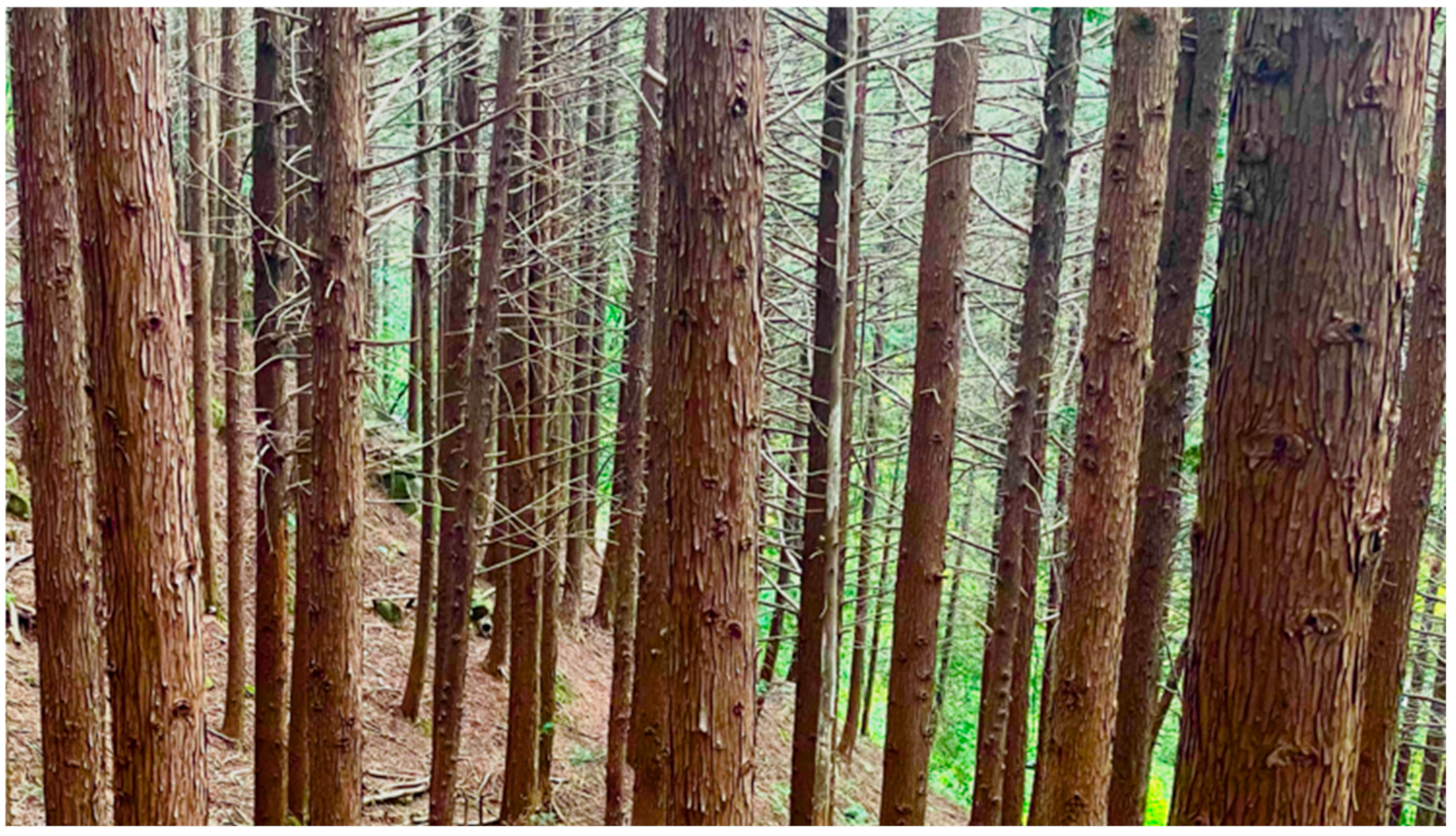
Forest stand structure is likely a key factor explaining this within-stand spatial variability because upper-canopy attributes, including canopy density and openness, can regulate rainfall interception and primary drip formation, whereas under-canopy elements can modify drip release height and the location of drip points above the forest floor. Previous studies have shown that vertical canopy structure can influence TKE in Japanese coniferous plantations [24,25], and that both upper- and lower-canopy structures may contribute to the spatial pattern of throughfall erosivity [17,18]. For example, previous work showed a strong relationship between distance from tree stems and TKE, suggesting that canopy architecture around tree stems may influence drip formation and raindrop delivery at the forest floor [6,26]. In unmanaged Japanese cypress plantations, densely attached dead branches resulting from a lack of pruning practices are a characteristic structural feature beneath the canopy and may provide additional drip points above the forest floor (Figure 1). Previous studies have suggested that dead branches play an important role in rainfall partitioning, including throughfall and stemflow [27], and may therefore influence local drip pathways and erosive forcing. Taken together, these findings suggest that dead branches may be associated with the spatial structure of TKE in unmanaged Japanese cypress plantations, although direct evidence remains limited [17].

Although much of the previous TKE literature for Japanese cypress plantations is based on studies in Japan, comparable unmanaged stand conditions are increasingly common in Korea [28]. In the Republic of Korea, forests occupy approximately 63% of the land area [29], and Japanese cypress plantations are widely distributed in southern regions [28,30,31]. Many of these plantations have reached or exceeded rotation age but remain unmanaged because of high management costs and limited economic returns [27,28,32]. Such conditions often result in persistent dead branches and heterogeneous vertical and under-canopy structures [27,33], providing a relevant setting for examining how stand structure influences the spatial variability of TKE beneath the canopy.

The main objective of this study was to clarify the spatial variability of TKE in unmanaged Japanese cypress stands and to identify the structural factors controlling this variability, with particular attention to the dead-branch layer and the lowest dead-branch height (H_db). To this end, we quantified TKE in two stands and examined whether forest stand structural attributes, including upper- and under-canopy characteristics, explained the observed within-stand variability in TKE. In addition, we compared the stand-mean TKE normalized with the corresponding total amount of rainfall (unit $\overline{\mathrm{T}\mathrm{K}\mathrm{E}}$) obtained in this study with previously reported values for Japanese cypress plantations to place our observations within the reported SD–TKE relationship.

2. Materials and Methods

2.1. Study Site

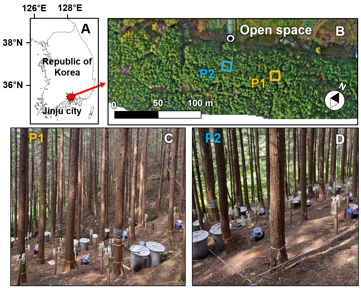
This study was conducted in Japanese cypress plantations at Mt. Seokgap (35°11′00″ N, 128°03′14″ E), Jinju city, Republic of Korea (167 m a.s.l.) (Figure 2A). The plantation is dominated by Japanese cypress, which was planted in March 1991 at an initial planting density of 3000 stems ha⁻¹. After a single thinning operation that reduced SD to approximately 2500 stems ha⁻¹, the site has remained unmanaged.

Climatic conditions were characterized using data from the nearest long-term meteorological station (Jinju city). The annual air temperature and precipitation were 13.4 ± 0.7 °C and 1518 ± 312 mm (mean ± standard deviation), respectively, based on records from 1999 to 2020 [34]. The regional climate includes a rainy season from June to September and a snowy season from December to February [34].

The study site is underlain by sedimentary rocks of the Cretaceous Jinju Formation, mainly sandstone and shale. The soil is generally loamy and developed from weathered sandstone and shale. For regional context, surface soils (0–30 cm) reported in the Jinju area are predominantly sandy loam, with bulk densities ranging from 1.06 to 1.13 g cm⁻³ [35].

Two 10 m × 10 m plots were established within the plantation (Figure 2B). Plot 1 (P1) was located on a slope of 19°, and Plot 2 (P2) was located on a slope of 29°. Each plot contained 25 trees, corresponding to 2500 stems ha⁻¹. Forest stand structure was summarized as (1) stand structure (tree number, age, plant area index (PAI), and density- and size-related attributes such as SD, diameter at breast height (DBH), basal area (BA)); (2) upper-canopy structure (structural characteristics of live branches and foliage), and (3) under-canopy structure (structural characteristics of dead branches beneath the canopy). The forest stand structure data are provided in

Table 1. Forest stand characteristics categorized into stand structure, upper-canopy structure, and under-canopy structure in two unmanaged Japanese cypress plantations.

Forest Stand Structure Variables	P1	P2	p
Stand structure
Tree age (yrs) 1	35	35	-
Stem density (SD, stems ha−1) 1	2500	2500	-
Diameter at breast height (DBH, cm) 2	19.1 ± 4.8	17.5 ± 4.2	0.202
Tree height (m) 2	19.7 ± 1.6	18.2 ± 2.0	0.006
Basal area (BA, m2 ha−1) 1	76.1	63.3	-
Plant area index (PAI, m2 m−2) 3	3.3 ± 0.1	3.7 ± 0.2	<0.001
Upper-canopy structure
No. of live branches (number tree−1) 2	20 ± 6	22 ± 5	0.360
Canopy projection area (CPA, m2) 2	8.1 ± 4.0	6.4 ± 3.7	0.134
Canopy cover (CC, %) 3	93.9 ± 0.7	95.3 ± 0.7	<0.001
Canopy bottom height (CBH, m) 2	14.9 ± 1.4	13.6 ± 1.8	0.009
Canopy length (CL, m) 2	4.8 ± 1.1	4.6 ± 1.4	0.563
Under-canopy structure
No. of dead branches (number tree−1) 2	45 ± 10	45 ± 8	0.702
Ratio of dead branches (%) 1	69.2	67.5	-
Lowest dead-branch height (Hdb, m) 3	9.4 ± 2.0	8.6 ± 3.3	0.395

Data are shown as mean ± standard deviation. Variables are grouped by measurement level as stand-level (¹), tree-level (²), and point-level (³) attributes. Stand-level variables are presented as single values for each plot. Tree-level variables were based on 25 trees per plot, and point-level variables were based on 20 points per plot. For replicated variables, differences between plots were evaluated using t-tests. PAI was treated as a stand-structure variable because it included both leaf and woody surface areas.

, and measurement procedures are described in Section 2.2.3.

2.2. Measurements

2.2.1. Gross Rainfall and Throughfall

The amount of gross rainfall (GR) was measured on an event basis using five manually read rain gauges (diameter: 7.8 cm). Each gauge was custom-made in-house from a plastic bottle fitted with a funnel and installed in an open space approximately 50 m and 30 m from P1 and P2, respectively. A rainfall event was defined as a period of rainfall separated from the next rainfall by at least 8 h without rainfall [27,36]. This threshold was selected in consideration of the commonly assumed canopy drying time (6–8 h) for Japanese cypress plantations in humid temperate climates [17,33]. The number of rainfall events during the observation period was determined using hourly rainfall data from the long-term meteorological station in Jinju City, located approximately 2.5 km southwest of the study site. Event-total GR measured using the manual gauges in the adjacent open space (GR_manual) closely agreed with the corresponding event-total rainfall recorded at the meteorological station (GR_station; GR_manual = 0.93 × GR_station, R² = 0.99).

Manual measurements of GR and TF were conducted from 28 June to 7 November in 2023, covering 14 rainfall events during the growing and rainy season. TF was measured using manual rain gauges (n = 20 per plot) during the same rainfall events for which GR was collected. The TF rain gauges were installed 70 cm above the forest floor to minimize splash contamination from the forest floor on sloping ground [17]. To ensure spatial representativeness within each plot, the 10 m × 10 m study area was divided into four equal subplots, and five TF rain gauges were installed within each subplot (20 points per plot). Stand-mean TF was calculated as follows:

$$\overline{\mathrm{T}\mathrm{F}}={\displaystyle \frac{{\displaystyle {\sum }_{\mathrm{i}=1}^{\mathrm{m}}}{\mathrm{T}\mathrm{F}}_{\mathrm{i}}}{\mathrm{m}}}$$

(1)

where $\overline{\mathrm{T}\mathrm{F}}$ is the stand-mean throughfall (mm) and $\mathrm{m}$ is the number of measurements taken from the plot (n = 20, each plot).

2.2.2. Splash Cup Measurements and Kinetic Energy Calculations

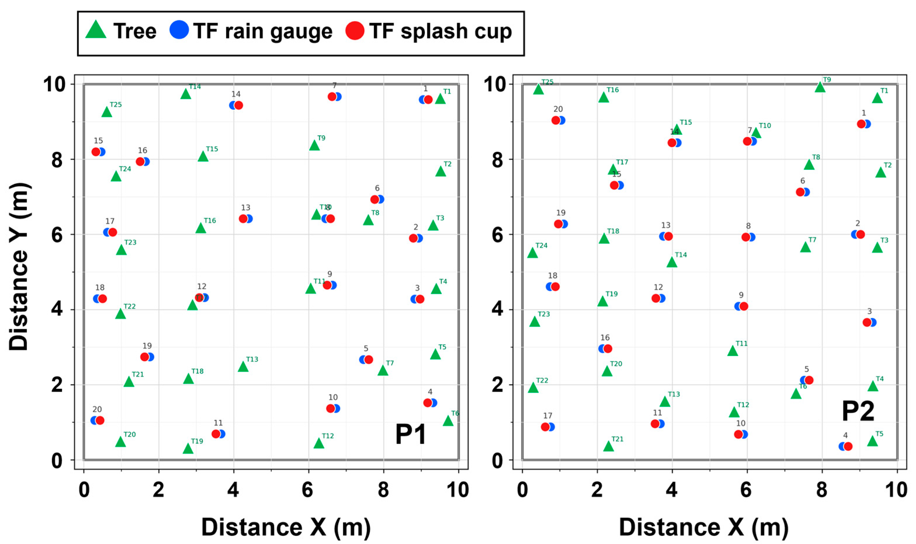
Sand-filled splash cups (diameter: 5.0 cm, height: 5.1 cm, volume: 100 cc) developed by Shinohara et al. [18], based on the Tübingen splash cup concept [37], were used to quantify splash-driven soil detachment. Each cup was filled with well-dried Toyoura standard sand (total mass of 155–160 g). Toyoura standard sand was used instead of the forest-floor material to provide a standardized detachment surface and to minimize variation caused by natural soil and organic-layer properties. Accordingly, the splash-cup-derived TKE should be interpreted as a standardized indicator of throughfall erosive forcing, rather than as a direct measurement of actual soil loss from the local forest floor [17]. In each plot, 20 sand-filled splash cups were pre-saturated with water and placed adjacent to the TF measurement points (Figure 3). The number of measurement points (n = 20) was selected to provide sufficient spatial coverage within each 10 m × 10 m plot while maintaining practical feasibility for repeated event-based sampling. Monte Carlo simulations in a recent study in an unmanaged Japanese cypress plantation laden with dead branches showed that a total sample size of 6–15 splash cups was appropriate for estimating mean TKE at the stand level with potential errors of ≤5%–10% [17]. Each cup was mounted on a 500 mL bottle to raise it above the forest floor and maintain stable placement on sloping ground. After each rainfall event, the splash cups were collected and returned to the laboratory, where the sand was dried at 105 °C for 24 h [6,17,38].

The loss of sand (LoS) was calculated as the difference in dry sand mass before and after each rainfall event. Kinetic energy (KE) was estimated from LoS using the empirical conversion equation proposed by Shinohara et al. [18] for the sand-filled splash cup method:

KE = 79.20 × LoS

(2)

where KE is kinetic energy (J m⁻²), and LoS is the mass of the loss of sand per splash cup (g). To quantify KE in the open space, five splash cups were installed for each rainfall event. Free kinetic energy (FKE) was calculated as the mean KE of these five cups.

Within each plot, TKE was estimated at each measurement location for each rainfall event by applying Equation (2) to the LoS measured in the corresponding under-canopy splash cup. Because Equation (2) is an empirical conversion from LoS, a zero LoS value was retained as zero splash-cup-derived KE/TKE in the calculations. This should be interpreted as indicating that no measurable sand detachment occurred within the sensitivity of the splash cup method, not that the physical kinetic energy of raindrops was necessarily zero. To evaluate the within-stand spatial variability of TKE, cumulative TKE at each measurement location was calculated by summing event-based TKE values across the same 14 rainfall events during which GR and TF were measured. Note that events with very small GR were included in the dataset, although their contribution to splash detachment by TF is considered minor [17].

To compare TKE among plots and with previous studies independently of rainfall amount, unit $\overline{\mathrm{T}\mathrm{K}\mathrm{E}}$ was calculated by normalizing the cumulative plot-mean TKE by total GR during the study period:

$$\mathrm{u}\mathrm{n}\mathrm{i}\mathrm{t} \overline{\mathrm{T}\mathrm{K}\mathrm{E}}={\displaystyle \frac{{\displaystyle {\sum }_{\mathrm{j}=1}^{\mathrm{n}}}{\displaystyle {\sum }_{\mathrm{i}=1}^{\mathrm{m}}}{\mathrm{T}\mathrm{K}\mathrm{E}}_{\mathrm{i}\mathrm{j}}}{\mathrm{m}{\displaystyle {\sum }_{\mathrm{j}=1}^{\mathrm{n}}}{\mathrm{G}\mathrm{R}}_{\mathrm{j}}}}$$

(3)

where unit $\overline{\mathrm{T}\mathrm{K}\mathrm{E}}$ is the plot-mean TKE normalized by total GR (J m⁻² mm⁻¹), ${\mathrm{T}\mathrm{K}\mathrm{E}}_{\mathrm{i}\mathrm{j}}$ is the TKE measured at location $\mathrm{i}$, during rainfall event $\mathrm{j}$ (J m⁻²), ${\mathrm{G}\mathrm{R}}_{\mathrm{j}}$ is the gross rainfall for event $\mathrm{j}$ (mm), $\mathrm{m}$ is the number of measurement locations in each plot ($\mathrm{m}$ = 20), and $\mathrm{n}$ is the number of rainfall events ($\mathrm{n}$ = 14). GR was used as the denominator because it is measured in the open and is independent of stand structure, allowing consistent comparison of throughfall erosivity across stands with different canopy and SD conditions. This normalization follows [19,25].

2.2.3. Forest Stand Structure

In this study, we measured the stand structure and the canopy structure divided into two components: upper-canopy structure (live branches with foliage) and under-canopy structure (dead branches without foliage). For stand-structure variables, DBH was measured for all standing trees at 1.3 m above the ground using a tree caliper. Tree height was measured for all trees using a Vertex IV hypsometer (Haglöf, Långsele, Sweden). BA was calculated from individual DBH measurements and expressed on a per-hectare basis. Unless otherwise noted, these stand-structure measurements were conducted in September 2023.

For the upper-canopy structure, the number of live branches of individual trees in each study plot was counted using a handheld telescope. The canopy projection area (CPA) was measured as the horizontal distance from each tree stem to the projected canopy edge in six compass directions (N, NE, SE, S, SW, NW) using diameter calipers. Canopy cover (CC) and PAI were derived from hemispherical photographs taken with an omnidirectional camera fitted with a fisheye lens (THETA SC; Ricoh Co., Ltd., Tokyo, Japan). Photographs were taken at the locations of the 20 TF manual rain gauges and 20 sand-filled splash cups under overcast conditions to minimize the effect of direct sunlight. CC and PAI were computed using Gap Light Analyzer ver. 2.0 [39]. PAI was treated as a stand-structure variable because it included both leaf and woody surface areas.

For the under-canopy structure, live and dead branches were distinguished visually with a telescope following [27]: branches longer than about 50 cm that retained foliage were regarded as live, and those without foliage as dead. This distinction is reliable in Japanese cypress because dead branches persist on the stem for years after foliage loss [32]. The number of dead branches of individual trees was then counted using a telescope. The ratio of dead branches was calculated as the number of dead branches divided by the total number of branches (live + dead branches). H_db was defined as the vertical distance from the ground surface to the lowest dead branch above each splash cup measurement point. H_db was measured at 20 measurement points per plot using a handheld hypsometer (manual clinometer height meter).

2.3. Method of Analysis

To check the difference in TF amounts in relation to GR between the two plots, the relationship between GR and TF was evaluated using linear regression for each plot. Differences in the GR–TF relationship between plots were tested using Analysis of Covariance (ANCOVA).

For cumulative FKE and TKE, the mean, standard deviation, range, and coefficient of variation were calculated across measurement locations. The coefficient of variation was calculated as CV = standard deviation/mean × 100%. Differences in cumulative TKE between P1 and P2 were tested using an independent-samples t-test.

To examine the factors associated with spatial variations in TKE within stands, three forest-stand variables measured at each TKE measurement point (Table 1) were examined as potential explanatory variables. Pearson’s correlation coefficients were calculated among these variables and TKE.

Spatial dependence in the focal H_db–TKE relationship was further evaluated separately for each plot by applying Moran’s I to the residuals of the ordinary least-square (OLS) regression, using a one-sided test for positive autocorrelation [40,41]. Spatial weights were constructed using a symmetrized k-nearest-neighbor scheme with row standardization, and the analysis was repeated for k = 3, 4, and 5 to assess sensitivity to the neighbor definition (R package spdep, version 1.4.2). Where significant positive residual spatial autocorrelation was detected, the H_db–TKE relationship was re-fitted using a spatial error model (SEM; R package spatialreg, version 1.4.3) [42], and model fit was compared with the OLS model using the Akaike information criterion (AIC). Because only two plots were available, a plot-level random intercept could not be estimated reliably; therefore, the H_db–TKE relationship was analyzed separately for each plot.

For comparison with previous Japanese cypress studies, previously reported unit $\overline{\mathrm{T}\mathrm{K}\mathrm{E}}$ values were extracted from Shinohara et al. [18] and Jeong et al. [19] and compared with the present data across a range of SD. Statistical significance was assessed at α = 0.05, and all analyses were performed in R (version 4.5.1).

3. Results

3.1. Gross Rainfall and Throughfall

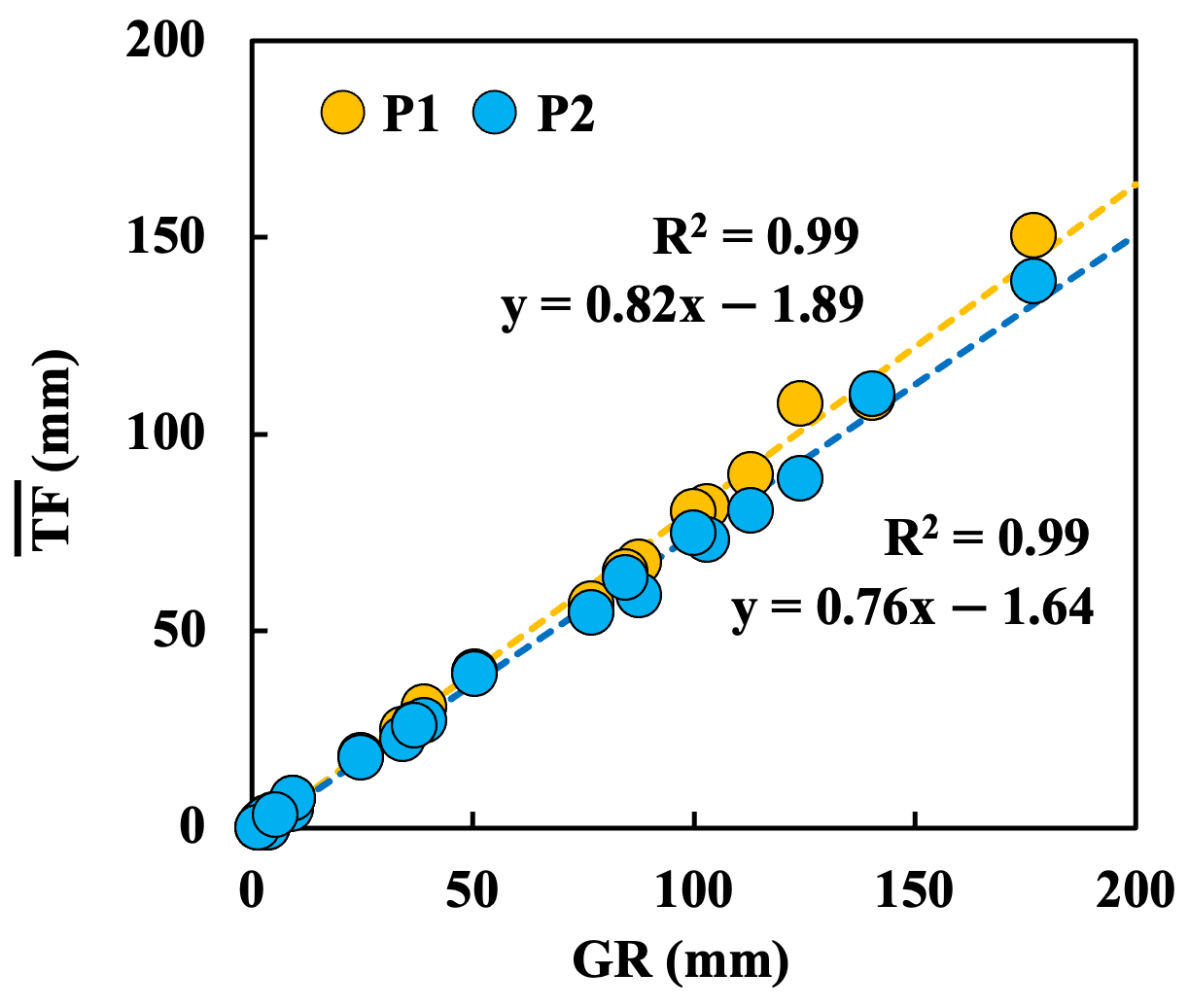
Event basis GR and $\overline{\mathrm{TF}}$ showed a strong linear relationship in both plots, indicating that TF increased consistently with GR during the observation period (Figure 4; R² > 0.99, p < 0.001). Total GR was 823.9 mm across 14 rainfall events (2.4–140.2 mm; mean 58.9 mm) (Table S1). Total $\overline{\mathrm{TF}}$ was 640.4 mm in P1 and 600.6 mm in P2, corresponding to 77.7% and 72.9% of GR, respectively. Although the GR–$\overline{\mathrm{TF}}$ slopes differed between plots (ANCOVA, plot × GR interaction: p < 0.001), the absolute difference was small (difference of the slopes: approximately 7.9% higher slope in P1 than in P2).

3.2. Free Kinetic Energy and Throughfall Kinetic Energy

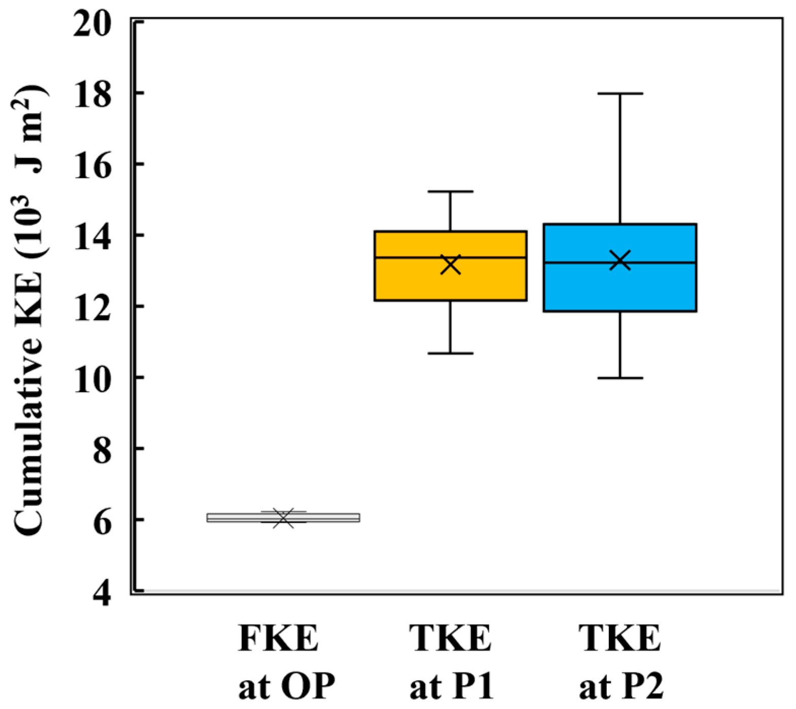
TKE and its variation in both plots were higher than those of FKE (Figure 5). FKE at the five open-space locations, summed across all rainfall events, ranged from 5928.6 to 6230.3 J m⁻², whereas TKE ranged from 10,678.0 to 15,212.8 J m⁻² in P1 and from 9988.2 to 17,971.2 J m⁻² in P2 (Figure 5; Table S1). The stand-mean cumulative TKE in P1 and P2 was 13,169.9 ± 1194.1 J m⁻² and 13,298.1 ± 2018.3 J m⁻², respectively, approximately 2.2 times higher than the mean FKE in the open space (6049.3 ± 118.4 J m⁻²). The stand-mean cumulative TKE did not differ significantly between the two plots (t-test, p = 0.81). TKE also showed greater variability beneath the canopy (CV = 9.1% in P1 and 15.2% in P2) than FKE in the open space (CV = 2.0%). The distributions of TKE were mostly similar between P1 and P2.

3.3. Relationships Between Forest Stand Variables and TKE

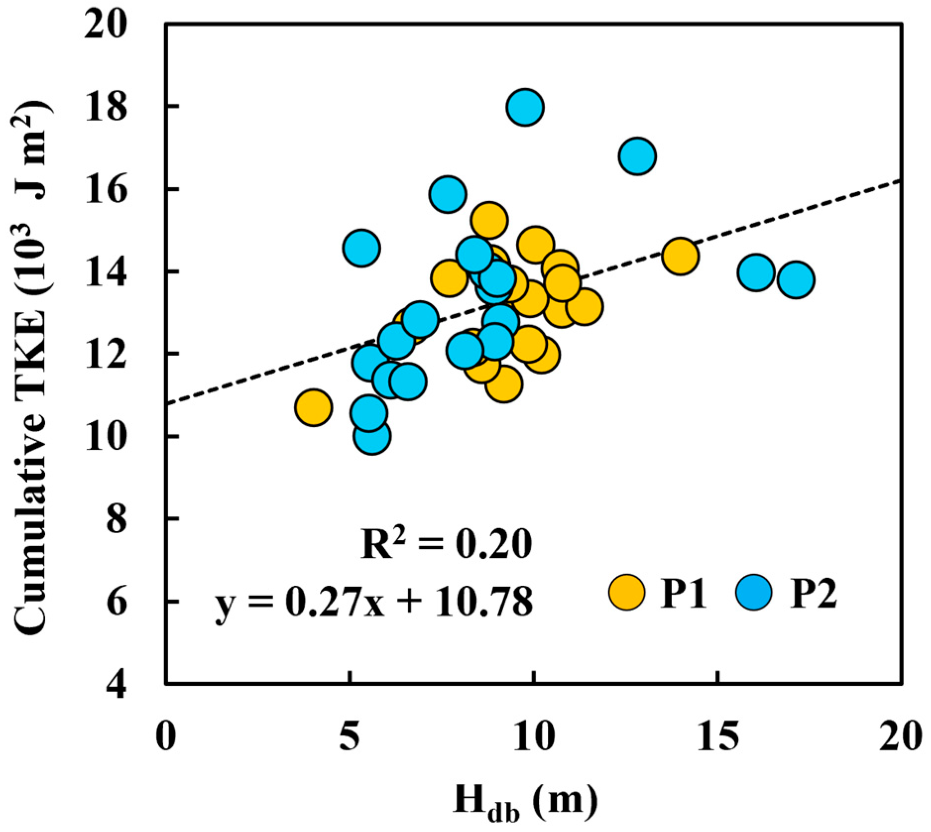
H_db showed a significant positive relationship with cumulative TKE at each measurement location (r = 0.447, p < 0.01;

Table 2. Pearson’s correlation coefficients among lowest dead-branch height (H_db, m), plant area index (PAI, m² m⁻²), canopy cover (CC, %) and TKE measured or calculated at the TKE measurement points.

Variable	Hdb	PAI	CC	Cumulative TKE
Hdb	1.000	−0.259 *	−0.142	0.447 ***
PAI	−0.259 *	1.000	0.836 ***	−0.041
CC	−0.142	0.836 ***	1.000	−0.019
Cumulative TKE	0.447 ***	−0.041	−0.019	1.000

*** p < 0.001, * p < 0.05. Correlations significant at p < 0.01 are indicated in bold.

; Figure 6). The relationship between H_db and TKE showed an overall increasing trend, although substantial dispersion remained across measurement points (R² = 0.20, p < 0.01; Figure 6). In contrast, PAI and CC were not significantly correlated with TKE (r = −0.041 and −0.019, respectively; Table 2). PAI and CC were strongly intercorrelated (r = 0.836, p < 0.001). H_db was weakly negatively correlated with PAI (r = −0.259, p < 0.05) and showed no significant correlation with CC (r = −0.142, p > 0.05).

Significant residual spatial autocorrelation was detected in the OLS residuals for P1 (Moran’s I = 0.388, p = 0.0002), whereas no significant spatial autocorrelation was detected for P2 (Moran’s I = −0.063, p = 0.5116;

Table 3. Spatial autocorrelation diagnostics and selected regression models for the relationship between lowest dead-branch height (H_db) and cumulative TKE.

Plot	Moran’s I of OLS Residuals	p-Value for Moran	Selected Model	Hdb Coefficient (J m−2 m−1)	p-Value for Hdb	λ	ΔAIC (SEM − OLS)
P1	0.388	0.0002	SEM	286.97	0.0030	0.636	−4.14
P2	−0.063	0.5116	OLS	333.50	0.0378	—	+1.76

Note: λ represents the spatial autoregressive coefficient describing residual spatial dependence in the SEM; it is not applicable to the OLS model.

). In P1, the SEM showed a significant positive association between H_db and TKE (coefficient = 286.97 J m⁻² m⁻¹, p = 0.003) and had a lower AIC than the OLS model (ΔAIC = −4.14). In P2, the OLS model showed a significant positive association between H_db and TKE (coefficient = 333.50 J m⁻² m⁻¹, p = 0.038), while the SEM had a higher AIC than the OLS model (ΔAIC = +1.76).

3.4. Unit $\overline{\mathit{TKE}}$ in Relation to Stem Density

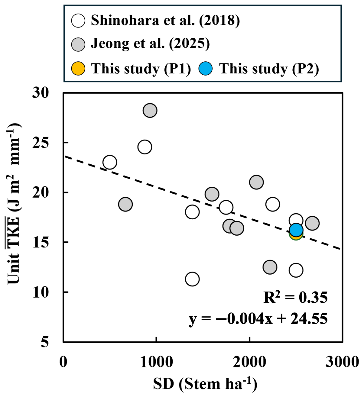
The unit $\overline{\mathrm{T}\mathrm{K}\mathrm{E}}$ values in the two plots were similar and fell within the range previously reported for Japanese cypress plantations at comparable SD (Figure 7). Previous studies showed a general decrease in unit $\overline{\mathrm{T}\mathrm{K}\mathrm{E}}$ with increasing SD across a wide SD range [17,18,19,25]. In the present study, unit $\overline{\mathrm{T}\mathrm{K}\mathrm{E}}$ was 16.0 J m⁻² mm⁻¹ in P1 and 16.1 J m⁻² mm⁻¹ in P2, closely matching the value predicted by the fitted SD–unit $\overline{\mathrm{T}\mathrm{K}\mathrm{E}}$ relationship at comparable SD (~2500 stems ha⁻¹).

4. Discussion and Conclusions

4.1. Canopy Enhancement of Throughfall Erosivity

The canopy substantially enhanced raindrop erosivity. TKE beneath the canopy was approximately twice as high as FKE measured in the open space (Figure 5). This indicates substantial canopy enhancement of raindrop-driven erosivity resulting from enlarged raindrop sizes within forest canopy [5]. This pattern is consistent with the established canopy effect whereby intercepted rainfall is temporarily stored, coalesces into larger drops, and is subsequently released to the forest floor with greater kinetic energy than open rainfall [11,12,15,17,18,43,44,45]. Thus, the canopy substantially modified the delivery of erosive energy to the soil surface.

4.2. Under-Canopy Structure and Spatial Variability in TKE

The clearest structural correlate of TKE was H_db (Table 2; Figure 6). This result suggests that the dead-branch layer, represented by H_db, may reflect part of the spatial organization of TKE within unmanaged Japanese cypress stands. To our knowledge, this is the first study to show a relationship between dead-branch distribution and TKE in unmanaged Japanese cypress stands. Although PAI and CC are commonly used to describe canopy structure and can influence throughfall partitioning and drip formation [17,18,19,20,23], neither variable was significantly correlated with TKE across the measurement locations (Table 2). This contrast suggests that, in the present unmanaged stands, spatial variation in TKE is more clearly associated with under-canopy structure, as represented by H_db, than with the measured upper-canopy attributes.

Dead branches beneath the canopy may intercept throughfall and alter subsequent drip formation. Water retained on woody surfaces in the under-canopy can be temporarily stored and subsequently released from different heights and positions, thereby changing local drop-forming conditions above the forest floor [6,22,23,26]. In Japanese cypress, branches are predominantly upward-facing in the upper canopy, whereas branch inclination decreases toward the lower canopy and some lower branches become downward-facing [46]. This vertical variation in branch orientation may influence whether intercepted water is retained and routed toward the stem or released more directly as throughfall drips; canopy saturation and branch position have also been shown to affect throughfall amount, drop characteristics, and kinetic energy [24,46]. In the present stands, each tree had approximately 45 dead branches (Table 1), indicating substantial structural complexity beneath the live canopy. Thus, orientation-dependent water retention and drainage within the dead-branch layer may modify local drip size and frequency.

Because release height and effective fall distance influence fall velocity and kinetic energy [15,18], the dead-branch layer may modify the impact energy of throughfall reaching the forest floor. Drops larger than approximately 3 mm in diameter require a fall distance of about 12 m before their velocity approaches the terminal value [47,48], and in an unmanaged Japanese cypress plantation 91% of throughfall drops in this size class reached the forest floor below 90% of terminal velocity [15]. This 12 m threshold provides a useful reference for interpreting the vertical structure of the present stands. In P1 and P2, mean CBH exceeded this threshold (14.9 ± 1.4 m in P1; 13.6 ± 1.8 m in P2), whereas mean H_db was 3–4 m below it (9.4 ± 2.0 and 8.6 ± 3.3 m; Table 1). Drops released from the live canopy could therefore approach terminal velocity if they fell without obstruction, but interception and re-release by dead branches would reduce the remaining uninterrupted fall distance to 8–9 m, and such drops would reach the forest floor while still accelerating. Points with a higher H_db would thus retain a longer uninterrupted fall distance and permit greater impact velocity, consistent with the observed positive H_db–TKE association.

This fall-distance interpretation is consistent with previous observations by Nanko et al. [15]. Nanko et al. [15] found that some throughfall drops fell more slowly than expected from the height of the lowest live branch and attributed this to drip generation from dead branches and near-stem surfaces. The present H_db–TKE relationship provides quantitative field evidence consistent with that inference. The H_db–TKE relationship explained only a modest proportion of the observed within-stand variation (R² = 0.20; Figure 6), indicating that H_db should be interpreted as a statistically significant structural correlate rather than as a dominant determinant of TKE. The positive association remained significant in P1 after residual spatial autocorrelation was accounted for using an SEM and was also significant in P2, where residual spatial autocorrelation was not detected (Table 3). This indicates that the observed H_db–TKE relationship was not solely attributable to spatial clustering among nearby measurement points. However, the persistence of the H_db–TKE association after accounting for spatial autocorrelation does not by itself establish the underlying drip-generation mechanism.

Direct measurements have shown that the presence or absence of foliage on branches alters throughfall drop-size distributions [23], which is consistent with the possibility that the leafless dead-branch layer modifies drip formation. However, because the present study estimated TKE using sand-filled splash cups, the actual drip sources, drop-size distributions, and fall velocities could not be resolved. In addition, the manual GR and TF gauges could not capture peak rainfall intensity or within-event rainfall dynamics, although rainfall intensity is a primary control on raindrop kinetic energy [49]. These measurement limitations prevented evaluation of event-scale processes such as canopy wetting, drainage, and temporal changes in drip formation. Therefore, targeted manipulation of the dead-branch layer, such as pruning, coupled with direct measurements of drop-size distributions and fall velocities using disdrometers and/or high-speed imaging, would provide a stronger test of drip-source dynamics and the delivery of kinetic energy at the forest floor [15,18,21,22].

4.3. Unit $\overline{\mathit{TKE}}$ in Relation to Stem Density

The unit $\overline{\mathrm{T}\mathrm{K}\mathrm{E}}$ values were nearly identical between the two plots (16.0 and 16.1 J m⁻² mm⁻¹) and fell within the range previously reported for Japanese cypress plantations at comparable SD (Figure 7). This comparison suggests that SD can be used as a stand-scale descriptor of mean throughfall erosivity [18,19,25], although SD should not be interpreted as a direct mechanistic control by itself. Instead, SD likely reflects integrated stand- and canopy-structural conditions, including planting density, canopy closure, LAI/PAI, canopy length, and canopy bottom height, which together may influence interception storage, drip coalescence, and effective drip release conditions [22,23,24,25]. However, the scatter in published relationships between SD and unit $\overline{\mathrm{T}\mathrm{K}\mathrm{E}}$ indicates that SD does not fully account for variation among stands [18,19,25].

Existing studies on Japanese cypress plantations have shown that branch-height-related variables can be associated with throughfall erosivity [17,18,25], but the structural meaning of these variables has not always been described consistently, particularly with respect to whether they represent live or dead branches. Future syntheses should explicitly document whether branch-height metrics refer to live or dead branches. In this context, broader comparisons or meta-analysis incorporating dead-branch height may help assess how general this pattern is across unmanaged Japanese cypress plantations. The comparison with previously reported unit $\overline{\mathrm{T}\mathrm{K}\mathrm{E}}$ values (Figure 7) places our data within the broader SD– unit $\overline{\mathrm{T}\mathrm{K}\mathrm{E}}$ relationship [18,19]. Because all values compiled in Figure 7 were normalized by gross rainfall, this comparison is not affected by differences in the normalization denominator. Nevertheless, this cross-study comparison provides broader context for the unit $\overline{\mathrm{T}\mathrm{K}\mathrm{E}}$ values observed in the present study but does not replace direct evaluation across an SD gradient within a single study. Accordingly, studies spanning a wider range of stem densities and stand structures are needed to confirm the generality of the observed H_db–TKE relationship and to support extrapolation to unmanaged Japanese cypress plantations.

A Japanese cypress (Chamaecyparis obtusa) plantation in Gochang, southern Korea, was reported to be located on slopes of 20–25° [50]. More broadly, national forest inventory data show that a substantial proportion of forest inventory plots in Korea are located on slopes exceeding 20°, including the 20–25° and 25–30° slope classes [51]. Taken together, these data suggest that the slopes of the present plots (19° and 29°) are broadly comparable to conditions reported for a Japanese cypress plantation in Korea and are not atypical within the broader topographic context of Korean forests. However, the available evidence does not establish that these two slope conditions are statistically representative of Japanese cypress plantations throughout South Korea. Because only one plot was established for each slope condition and both plots had the same stem density (2500 stems ha⁻¹), the study provided neither independent replication across slope conditions nor a within-study SD gradient. Nevertheless, the positive H_db–TKE association detected in both plots indicates a consistent pattern within the study site. Additional observations from independent stands across a broader range of slope conditions would help evaluate the wider applicability of this relationship.

Overall, the present results suggest that SD is useful for characterizing the stand mean TF erosivity, whereas under-canopy structure, including the dead-branch layer, is associated with within-stand spatial heterogeneity in unmanaged Japanese cypress stands. Because the splash cups used standardized Toyoura sand, the measured TKE represents throughfall erosivity rather than the erodibility of the local forest floor. Actual splash erosion also depends on forest-floor conditions, such as litter cover, soil moisture, aggregate stability, and surface roughness, and therefore cannot be inferred directly from the measured TKE. From a management perspective, thinning may alter stand-level rainfall partitioning [52] and potentially affect mean erosivity. However, the present results also suggest that the layer of dead branches should be considered when evaluating localized throughfall erosivity and potential splash erosion risk in unmanaged or partially managed Japanese cypress stands [53].

References

1. Kinnell, P.I.A. Raindrop-impact-induced erosion processes and prediction: A review. Hydrol. Processes 2005, 19, 2815–2844. [Google Scholar] [CrossRef]
2. Mohammad, H.; Assefa, M.M.; Hector, R.F. Raindrop-Induced Erosion and Sediment Transport Modelling in Shallow Waters: A Review. J. Soil Water Sci. 2018, 1, 15–25. [Google Scholar] [CrossRef]
3. Zhang, X.J. Roles of raindrop impact in detachment and transport processes of interrill soil erosion. Int. Soil Water Conserv. Res. 2023, 11, 592–601. [Google Scholar] [CrossRef]
4. Miura, S.; Hirai, K.; Yamada, T. Transport Rates of Surface Materials on Steep Forested Slopes Induced by Raindrop Splash Erosion. J. For. Res. 2002, 7, 201–211. [Google Scholar] [CrossRef]
5. Nanko, K.; Hotta, N.; Suzuki, M. Assessing raindrop impact energy at the forest floor in a mature Japanese cypress plantation using continuous raindrop-sizing instruments. J. For. Res. 2004, 9, 157–164. [Google Scholar] [CrossRef]
6. Katayama, A.; Nanko, K.; Jeong, S.; Kume, T.; Shinohara, Y.; Seitz, S. Short communication: Concentrated impacts by tree canopy drips—Hotspots of soil erosion in forests. Earth Surf. Dyn. 2023, 11, 1275–1282. [Google Scholar] [CrossRef]
7. Morgan, R.P.C. Soil Erosion and Conservation, 3rd ed.; Blackwell Publishing Ltd.: Malden, MA, USA, 2005. [Google Scholar]
8. Miura, S.; Ugawa, S.; Yoshinaga, S.; Keizo Hirai, T.Y. Floor Cover Percentage Determines Splash Erosion in Chamaecyparis obtusa Forests. Soil Sci. Soc. Am. J. 2015, 79, 1782–1791. [Google Scholar] [CrossRef]
9. Nanko, K.; Hotta, N.; Suzuki, M. Evaluating the influence of canopy species and meteorological factors on throughfall drop size distribution. J. Hydrol. 2006, 329, 422–431. [Google Scholar] [CrossRef]
10. Goebes, P.; Bruelheide, H.; Hardtle, W.; Krober, W.; Kuhn, P.; Li, Y.; Seitz, S.; von Oheimb, G.; Scholten, T. Species-Specific Effects on Throughfall Kinetic Energy in Subtropical Forest Plantations Are Related to Leaf Traits and Tree Architecture. PLoS ONE 2015, 10, e0128084. [Google Scholar] [CrossRef] [PubMed]
11. Goebes, P.; Seitz, S.; Kühn, P.; Li, Y.; Niklaus, P.A.; Oheimb, G.v.; Scholten, T. Throughfall kinetic energy in young subtropical forests: Investigation on tree species richness effects and spatial variability. Agric. For. Meteorol. 2015, 213, 148–159. [Google Scholar] [CrossRef]
12. Ji, S.; Omar, S.I.; Zhang, S.; Wang, T.; Chen, C.; Zhang, W. Comprehensive evaluation of throughfall erosion in the banana plantation. Earth Surf. Processes Landf. 2022, 47, 2941–2949. [Google Scholar] [CrossRef]
13. Onda, Y.; Gomi, T.; Mizugaki, S.; Nonoda, T.; Sidle, R.C. An overview of the field and modelling studies on the effects of forest devastation on flooding and environmental issues. Hydrol. Processes 2010, 24, 527–534. [Google Scholar] [CrossRef]
14. Geißler, C.; Nadrowski, K.; Kuhn, P.; Baruffol, M.; Bruelheide, H.; Schmid, B.; Scholten, T. Kinetic energy of Throughfall in subtropical forests of SE China-effects of tree canopy structure, functional traits, and biodiversity. PLoS ONE 2013, 8, e49618. [Google Scholar] [CrossRef] [PubMed]
15. Nanko, K.; Mizugaki, S.; Onda, Y. Estimation of soil splash detachment rates on the forest floor of an unmanaged Japanese cypress plantation based on field measurements of throughfall drop sizes and velocities. Catena 2008, 72, 348–361. [Google Scholar] [CrossRef]
16. Nanko, K.; Giambelluca, T.W.; Sutherland, R.A.; Mudd, R.G.; Nullet, M.A.; Ziegler, A.D. Erosion Potential under Miconia calvescens Stands on the Island of Hawai‘i. Land Degrad. Dev. 2015, 26, 218–226. [Google Scholar] [CrossRef]
17. Jeong, S.; Nanko, K.; Katayama, A.; Kume, T.; Koga, S.; Otsuki, K. Characteristics of throughfall kinetic energy in an unmanaged Japanese cypress plantation laden with dead branches. Catena 2024, 243, 108181. [Google Scholar] [CrossRef]
18. Shinohara, Y.; Ichinose, K.; Morimoto, M.; Kubota, T.; Nanko, K. Factors influencing the erosivity indices of raindrops in Japanese cypress plantations. Catena 2018, 171, 54–61. [Google Scholar] [CrossRef]
19. Jeong, S.; Li, Y.; Kamitani, R.; Chiwa, M.; Otsuki, K. Naturally grown understory vegetation after thinning reduces throughfall erosivity in Japanese coniferous plantations. J. Agric. Meteorol. 2025, 81, 117–125. [Google Scholar] [CrossRef]
20. Levia, D.F., Jr.; Frost, E.E. Variability of throughfall volume and solute inputs in wooded ecosystems. Prog. Phys. Geogr. Earth Environ. 2006, 30, 605–632. [Google Scholar] [CrossRef]
21. Levia, D.F.; Hudson, S.A.; Llorens, P.; Nanko, K. Throughfall drop size distributions: A review and prospectus for future research. WIREs Water 2017, 4, e1225. [Google Scholar] [CrossRef]
22. Levia, D.F.; Nanko, K.; Amasaki, H.; Giambelluca, T.W.; Hotta, N.; Iida, S.i.; Mudd, R.G.; Nullet, M.A.; Sakai, N.; Shinohara, Y.; et al. Throughfall partitioning by trees. Hydrol. Processes 2019, 33, 1698–1708. [Google Scholar] [CrossRef]
23. Nanko, K.; Hudson, S.A.; Levia, D.F. Differences in throughfall drop size distributions in the presence and absence of foliage. Hydrol. Sci. J. 2016, 61, 620–627. [Google Scholar] [CrossRef]
24. Nanko, K.; Onda, Y.; Ito, A.; Moriwaki, H. Effect of canopy thickness and canopy saturation on the amount and kinetic energy of throughfall: An experimental approach. Geophys. Res. Lett. 2008, 35, L05401. [Google Scholar] [CrossRef]
25. Nanko, K. Relationship between Throughfall Kinetic Energy and Tree Height, Crown Bottom Height, and Crown Length for Japanese Cypress Plantation. J. Jpn. For. Soc. 2013, 95, 234–239. [Google Scholar] [CrossRef]
26. Nanko, K.; Keim, R.F.; Hudson, S.A.; Levia, D.F. Throughfall drop sizes suggest canopy flowpaths vary by phenophase. J. Hydrol. 2022, 612, 128144. [Google Scholar] [CrossRef]
27. Jeong, S.; Otsuki, K.; Inoue, A.; Shinohara, Y. Marked difference of rainfall partitioning in an unmanaged coniferous plantation with high stand density. J. For. Res. 2019, 24, 107–114. [Google Scholar] [CrossRef]
28. Park, S.-G.; Kang, H.-M. Characteristics of Vegetation Structure in Chamaecyparis obtusa Stands. Korean J. Environ. Ecol. 2015, 29, 907–916. [Google Scholar] [CrossRef]
29. Korea Forest Service. Statistical Yearbook of Forestry 2020; Korea Forest Service: Daejeon, Republic of Korea, 2020. [Google Scholar]
30. Lee, J.; Cho, K.S.; Jeon, Y.; Kim, J.B.; Lim, Y.-r.; Lee, K.; Lee, I.-S. Characteristics and distribution of terpenes in South Korean forests. J. Ecol. Environ. 2017, 41, 19. [Google Scholar] [CrossRef]
31. Korea Forest Service. Statistical Yearbook of Forestry 2024; Korea Forest Service: Daejeon, Republic of Korea, 2024. [Google Scholar]
32. Fujimori, T. Dynamics of crown structure and stem growth based on knot analysis of a hinoki cypress. For. Ecol. Manag. 1993, 56, 57–68. [Google Scholar] [CrossRef]
33. Jeong, S.; Kume, T.; Shinohara, Y.; Farahnak, M.; Otsuki, K. Application of the Reformulated Gash Analytical Model for Rainfall Interception Loss to Unmanaged High-Density Coniferous Plantations Laden with Dead Branches. Forests 2022, 13, 657. [Google Scholar] [CrossRef]
34. Korea Meteorological Administration. Climatological Data of Jinju Station (1999–2020); Korea Meteorological Administration: Seoul, Republic of Korea, 2021.
35. An, S.E.; Lee, J.; Kim, C. Relationships between Soil Carbon Storage and Soil Properties of Urban Parks in Jinju-si, Gyeongsangnam-do. Korean J. Agric. For. Meteorol. 2022, 24, 115–123. [Google Scholar] [CrossRef]
36. Shinohara, Y.; Levia, D.F.; Komatsu, H.; Nogata, M.; Otsuki, K. Comparative modeling of the effects of intensive thinning on canopy interception loss in a Japanese cedar (Cryptomeria japonica D. Don) forest of western Japan. Agric. For. Meteorol. 2015, 214–215, 148–156. [Google Scholar] [CrossRef]
37. Scholten, T.; Geißler, C.; Goc, J.; Kühn, P.; Wiegand, C. A new splash cup to measure the kinetic energy of rainfall. J. Plant Nutr. Soil Sci. 2011, 174, 596–601. [Google Scholar] [CrossRef]
38. Liu, J.; Liu, W.; Li, W.; Jiang, X.; Wu, J. Effects of rainfall on the spatial distribution of the throughfall kinetic energy on a small scale in a rubber plantation. Hydrol. Sci. J. 2018, 63, 1078–1090. [Google Scholar] [CrossRef]
39. Frazer, G.W.; Canham, C.D.; Lertzman, K.P. Gap Light Analyzer (GLA) Version 2.0: Imaging Software to Extract Canopy Structure and Gap Light Transmission Indices from True-Colour Fisheye Photographs, User’s Manual and Program Documentation; Simon Fraser University: Burnaby, BC, Canada; The Institute of Ecosystem Studies: Millbrook, NY, USA, 1999. [Google Scholar]
40. Cliff, A.D.; Ord, J.K. Spatial Processes: Models & Applications; Pion: London, UK, 1981; p. 266. [Google Scholar]
41. Bivand, R.S.; Wong, D.W.S. Comparing implementations of global and local indicators of spatial association. Test 2018, 27, 716–748. [Google Scholar] [CrossRef]
42. Anselin, L. Spatial Econometrics: Methods and Models, 1st ed.; Springer: Dordrecht, The Netherlands, 1988; Volume 4, p. 284. [Google Scholar]
43. Brandt, C.J. The size distribution of throughfall drops under vegetation canopies. Catena 1989, 16, 507–524. [Google Scholar] [CrossRef]
44. Liu, J.; Liu, W.; Zhu, K. Throughfall kinetic energy and its spatial characteristics under rubber-based agroforestry systems. Catena 2018, 161, 113–121. [Google Scholar] [CrossRef]
45. Mosley, M.P. The effect of a New Zealand beech forest canopy on the kinetic energy of water drops and on surface erosion. Earth Surf. Processes Landf. 1982, 7, 103–107. [Google Scholar] [CrossRef]
46. Nanko, K.; Onda, Y.; Ito, A.; Moriwaki, H. Spatial variability of throughfall under a single tree: Experimental study of rainfall amount, raindrops, and kinetic energy. Agric. For. Meteorol. 2011, 151, 1173–1182. [Google Scholar] [CrossRef]
47. Wang, P.K.; Pruppacher, H.R. Acceleration to Terminal Velocity of Cloud and Raindrops. J. Appl. Meteorol. 1977, 16, 275–280. [Google Scholar] [CrossRef] [PubMed]
48. Laws, J.O. Measurements of the Fall-Velocity of Water-Drops and Raindrops. Trans. Am. Geophys. Union 1941, 22, 709–721. [Google Scholar] [CrossRef]
49. van Dijk, A.I.J.M.; Bruijnzeel, L.A.; Rosewell, C.J. Rainfall intensity–kinetic energy relationships: A critical literature appraisal. J. Hydrol. 2002, 261, 1–23. [Google Scholar] [CrossRef]
50. Lee, J.-G.; Lee, D.-H.; Jung, J.-Y.; Lee, S.-G.; Han, S.H.; Kim, S.; Kim, H.-J. The Effects of Stand Density Control on Carbon Cycle in Chamaecyparis obtusa (Siebold and Zucc.) Endl. Forests. Forests 2023, 14, 217. [Google Scholar] [CrossRef]
51. Korea Forest Research Institute. 2006–2010 The 5th National Forest Inventory Report; Korea Forest Research Institute: Seoul, Republic of Korea, 2011; pp. 28–29.
52. Sun, X.; Onda, Y.; Kato, H.; Gomi, T.; Komatsu, H. Effect of strip thinning on rainfall interception in a Japanese cypress plantation. J. Hydrol. 2015, 525, 607–618. [Google Scholar] [CrossRef]
53. Komatsu, H.; Shinohara, Y.; Otsuki, K. Models to predict changes in annual runoff with thinning and clearcutting of Japanese cedar and cypress plantations in Japan. Hydrol. Processes 2015, 29, 5120–5134. [Google Scholar] [CrossRef]
Figure 1. Under-canopy dead-branch layer and forest floor conditions in an unmanaged Japanese cypress plantation.
Forests 17 00848 g001
Figure 2. Study site at Mt. Seokgap, Jinju city, Republic of Korea. (A) Geographic location of the study site. (B) Orthophotograph showing two study plots (P1, P2) and the open space at Mt. Seokgap. Forest floor conditions and experimental setup in P1 (C) and P2 (D).
Forests 17 00848 g002
Figure 3. Experimental layout of throughfall rain gauges, splash cups, and tree locations in the two 10 m × 10 m study plots. Blue circles indicate throughfall rain gauges, red circles indicate splash cups, and green triangles indicate tree locations. Numbers indicate paired throughfall–splash measurement points.
Forests 17 00848 g003
Figure 4. Relationship between gross rainfall (GR) and stand-mean throughfall ( T F ¯ ) for P1 and P2.
Forests 17 00848 g004
Figure 5. Comparison of free kinetic energy (FKE) and throughfall kinetic energy (TKE) summed across all rainfall events at five open-space locations and 20 TKE measurement locations in P1 and P2, respectively. Boxes represent the interquartile range with the median (central line); whiskers denote the minimum and maximum, and crosses (×) the mean. P1 and P2 are shown in yellow and blue, respectively.
Forests 17 00848 g005
Figure 6. Relationship between Hdb and TKE summed across all rainfall events at the measurement locations in P1 and P2.
Forests 17 00848 g006
Figure 7. Relationship between stem density (SD) and unit T K E ¯ in Japanese cypress plantations, including P1 and P2. The dashed line represents linear regression calculated from the plotted data. Previously reported values were obtained from Shinohara et al. [18] and Jeong et al. [19] All unit T K E ¯ values were normalized by GR. Values for Shinohara et al. [18] were computed as KE (=79.20 × loss of sand) divided by the open-space GR reported for each plot.
Forests 17 00848 g007