How Do High- and Low-Canopy Landscape Patterns Affect Human Heat Exposure? Mechanisms and Regional Heterogeneity in Chinese Cities, 2000–2020

Abstract

Urban canopy mitigates urban heat, yet how the spatial configuration of high- and low-canopy layers shapes population heat exposure across a national urban system remains insufficiently understood. Drawing on a panel of 369 Chinese prefecture-level cities for 2000, 2005, 2010, 2015, and 2020, this study constructs a population-weighted thermal-exposure metric—the Human Heat Exposure Index (HEI)—and stratifies urban vegetation into high- and low-canopy classes based on Chinese Land Cover Dataset (CLCD) land-cover types. Multiscale Geographically Weighted Regression (MGWR) and Extreme Gradient Boosting (XGBoost) with SHapley Additive exPlanations (SHAP)-based interpretation are combined to identify spatially varying associations and nonlinear marginal effects of stratified canopy patterns on HEI. HEI shows a persistent south–high, north–low spatial structure, with Global Moran’s I stable at approximately 0.85 throughout the study period. High-canopy edge density and cohesion are increasingly associated with reduced heat exposure in densely built regions, while low-canopy mean patch area and edge density retain explanatory power across all years through near-surface evapotranspirative regulation. The marginal cooling effect of vegetation strengthens appreciably only above an Normalized Difference Vegetation Index (NDVI) of approximately 0.6, and the apparent inflection ranges for impervious surface proportion and standardized solar radiation lie near 25% and 0.4, respectively. These findings suggest that in cities with high impervious loads, cooling-network connectivity and within-zone canopy configuration matter more than additional canopy area alone, and that planning targets should be calibrated to climate zone, city type, and existing surface conditions.

1. Introduction

With the accelerating pace of global urbanization, urban surfaces are increasingly being covered by impervious materials, making the urban heat island effect ever more pronounced. Extreme heat events have become more frequent and intense, further amplifying population heat exposure risks under conditions of dense urban settlement [1,2]. Under the combined pressures of climate change and high-density urban development, mitigating population heat exposure and building heat-resilient cities have become major research priorities [3]. Two well-established biophysical mechanisms underpin vegetation-induced cooling: (i) interception of incoming shortwave solar radiation by leaf canopies, which reduces surface heat absorption and the resulting longwave re-emission, and (ii) latent heat exchange through evapotranspiration, which converts sensible-to-latent heat at the leaf–air interface and lowers near-surface air temperature. Recent quasi-experimental and remote sensing studies have demonstrated that these mechanisms generate substantial daytime cooling at the city scale, with cooling magnitudes ranging from 0.5 to over 4 °C, depending on the canopy density and climatic context [4,5,6]. Vegetation thus directly modulates the radiative- and latent-heat budgets of urban surfaces, providing the mechanistic foundation for the statistical associations explored in this study.

Characterizing the actual heat burden experienced by urban residents requires a metric that couples thermal intensity with population distribution, rather than relying on temperature fields alone. The established literature has addressed this need through the population-weighted mean land surface temperature, operationalized as the Human Heat Exposure Index (HEI) [7,8] and adopted in subsequent inter-city comparative studies as a macro-scale exposure indicator [9]. It is important to be explicit about what this index measures and what it does not. HEI captures the aggregate thermal load experienced by a city’s population, weighting hotter pixels more heavily when they coincide with higher population density; it does not purport to represent perceived thermal comfort at the individual scale, which requires the integration of air temperature, humidity, wind speed, mean radiant temperature, and metabolic assumptions, as in the Universal Thermal Climate Index (UTCI) or Physiological Equivalent Temperature (PET). The choice of HEI over UTCI or PET in this study is not a conceptual oversight but a deliberate methodological constraint: gridded, sub-daily meteorological fields at the spatial resolution and temporal span required to compute UTCI across 369 cities over five epochs are not available with the consistency needed for a national panel analysis, whereas MODIS LST composites and LandScan population grids provide spatially and temporally consistent inputs throughout 2000–2020.

Among the various approaches to regulating the urban thermal environment, urban vegetation is widely regarded as one of the most economical and sustainable nature-based cooling solutions [10]. Existing studies generally demonstrate that urban vegetation plays a significant role in reducing land surface temperature and improving the thermal environment. However, its cooling performance depends not only on total vegetation area, but also on how canopy is spatially organized [11]. From the perspective of landscape ecology, patch size, fragmentation, shape complexity, aggregation, and connectivity can influence heat exchange, airflow, and the diffusion of cooling effects, thereby altering cooling efficiency [12].

Existing research on urban vegetation has largely remained within a two-dimensional perspective, treating green space as a relatively homogeneous whole while paying limited attention to differences in thermal regulation among vegetation types with different vertical structures [13,14]. In reality, urban vegetation exhibits clear vertical heterogeneity, and high- and low-canopy areas differ fundamentally in spatial form, ecological function, and cooling mechanisms. High-canopy areas exert their effects through three-dimensional shading and canopy regulation, whereas low-canopy areas rely more on near-surface evapotranspiration and ground-cover effects to influence the local microclimate [15,16]. This suggests that a focus solely on a two-dimensional area or planar landscape pattern is insufficient to fully reveal the mechanisms through which urban vegetation affects heat exposure.

Although the literature on three-dimensional canopy structure has expanded with the advent of GEDI and ICESat-2 LiDAR products [17,18,19], national-scale and multi-temporal evidence on how stratified canopy patterns shape population heat exposure across Chinese cities remains scarce. Most existing studies are restricted to single cities, single epochs, or coarse two-dimensional vegetation indices, and few link a stratified canopy configuration to a population-weighted exposure metric over a 20-year window. We acknowledge that our stratification, derived from land-cover categories, is an indirect proxy for genuine three-dimensional canopy structure; the integration of GEDI/LiDAR-derived 3D canopy attributes is treated as a future research priority [20].

Against this background, this study integrates multi-source remote sensing data, population distribution data, and geographic information from 2000 to 2020 across 369 Chinese prefecture-level cities to construct HEI and systematically examine the effects of stratified canopy landscape patterns on population-weighted thermal exposure. The analytical framework combines MGWR with XGBoost–SHAP, characterizing the spatial heterogeneity, nonlinear associations, and scale-dependent patterns through which high- and low-canopy landscape configuration influences HEI, thereby providing geographically differentiated guidance for the optimization of urban green space toward greater heat resilience.

This study addresses two key questions: (1) How do the spatial patterns of urban vegetation affect population heat exposure in Chinese cities? (2) How have these effects evolved spatially and temporally over the past two decades? The findings are expected to provide scientific guidance for climate change adaptation and the optimization of urban spatial structure.

2. Theoretical Background and Literature Review

2.1. Cooling Effects of Urban Vegetation

Urban canopy constitutes an important ecological component in mitigating urban heat, and its cooling effects mainly arise from evapotranspiration and shading [21]. During evapotranspiration, plants consume ambient heat and remove part of the thermal energy through latent heat exchange, thereby reducing the surrounding air temperature. At the same time, vegetation canopies intercept incoming shortwave solar radiation, decrease surface heat absorption, and consequently suppress increases in land surface temperature [4]. In addition, canopy can exert sustained influences on the local microclimate by altering underlying surface properties and regulating near-surface airflow and humidity conditions. For these reasons, urban canopy has long been regarded as key ecological infrastructure for mitigating the urban heat island effect, improving thermal environmental quality, and enhancing urban heat resilience.

The benefits of urban canopy extend beyond temperature reduction to the human dimension of heat risk, because population heat exposure, unlike thermal intensity alone, emphasizes the spatial coincidence of high temperature with population concentration, and the Human Heat Exposure Index adopted here—the population-weighted mean land surface temperature within each city, following Tuholske et al. [7] and Chakraborty et al. [8]—reflects this aggregate dimension and is an existing operational metric rather than a new index. By improving the local thermal environment and reducing heat accumulation, denser and better-configured canopy lowers the land surface temperature experienced by residents in the most heavily loaded pixels and thereby reshapes the spatial distribution of HEI, and because this metric differs in purpose and data requirements from individual-level comfort indices such as UTCI and PET, the detailed rationale for adopting it in a national, multi-temporal panel is given in Section 3.2.1 [5,22].

Meanwhile, existing studies still rely heavily on aggregate indicators such as area proportion in variable selection. Although these indicators can reflect canopy extent, they are insufficient for fully capturing the effects of patch fragmentation, edge effects, and spatial connectivity on heat exchange processes [23]. It is therefore necessary to further incorporate landscape metrics such as patch density, connectivity, and shape index in order to identify, from a more refined landscape perspective, the differences in how various canopy types mitigate population heat exposure. More importantly, canopy is not a single ecological element with internally uniform functions. Different canopy layers may differ substantially in both their thermal regulation pathways and their effectiveness in alleviating heat exposure, which also provides the basis for the subsequent discussion of performance differences among stratified canopy.

2.2. Performance Differences Between High- and Low-Canopy Vegetation

Although the cooling effects of urban canopy have been widely documented, existing studies still tend to treat canopy as a relatively homogeneous whole at the conceptual level, with greater emphasis placed on total area or overall coverage than on the functional differences among canopy layers [17]. In reality, urban canopy is not a single homogeneous ecological entity, but rather a composite system with clear stratified characteristics. Different canopy layers differ fundamentally in morphological structure, modes of energy exchange, and pathways of microclimate regulation. High-canopy areas usually provide stronger canopy cover and can exert relatively stable thermal regulation by expanding shaded areas, reducing incoming shortwave solar radiation, and, to some extent, modifying local ventilation conditions. In contrast, low-canopy areas are located closer to the ground surface, and their cooling effects depend primarily on near-surface evapotranspiration and ground-cover processes, making their mitigation of local heat accumulation more surface oriented and context dependent [6].

Taken together, the differences among canopy layers are not merely differences in cooling intensity, but also reflect substantial divergence in regulatory pathways, the spatial extent of influence, and modes of spatial response. If the effects of canopy are assessed only by the overall greening rate or total green space area, such measures may capture the overall scale of the urban ecological space, but they cannot adequately reveal the functional differentiation of stratified canopy in thermal regulation, nor can they explain the differentiated effects of different canopy layers on mitigating population heat exposure. Therefore, re-examining the thermal regulatory performance of urban canopy from the perspective of stratified structure is an essential prerequisite for deepening our understanding of the ecological mechanisms through which urban environments regulate population heat exposure.

2.3. Identification Approaches Based on Interpretable Machine Learning

From a methodological perspective, accurately identifying the complex relationship between vegetation patterns and population heat exposure remains a major challenge in this field. Although traditional linear regression models offer strong interpretability, they are generally limited in their ability to capture the spatial non-stationarity of geographic data and the potential nonlinear relationships among variables [24]. Geographically weighted regression and its extended forms are better suited to revealing the spatial heterogeneity of effects across different regional contexts, but they still have certain limitations in identifying complex nonlinear responses and multi-factor interactions [25].

In recent years, machine learning methods such as Random Forest and Extreme Gradient Boosting have been widely applied in thermal environment studies because of their strong adaptability to high-dimensional nonlinear relationships [26]. When combined with interpretability frameworks such as SHAP, these methods can not only rank the relative contributions of different factors but also more precisely identify the nonlinear marginal effects of landscape metrics on cooling efficiency. A persistent methodological concern with the application of these models to spatially structured data, however, is that ignoring spatial autocorrelation among observations can lead to inflated apparent predictive performance and spurious feature importance rankings, because nearby cities share climatic and geographic conditions that the model may learn without those features being causally relevant. This study addresses this concern explicitly through climate-zone-stratified cross-validation, which ensures that cities from the same climatic background are not simultaneously present in training and validation folds, thereby providing a more conservative and geographically honest assessment of out-of-sample model performance.

Overall, the existing literature still suffers from several limitations. First, most studies use land surface temperature or air temperature as the main indicators of the thermal environment and primarily focus on the temperature-regulating effects of canopy. By contrast, relatively few studies examine population heat exposure from the perspective of the coupling between thermal conditions and population distribution, and thus the mechanisms through which canopy mitigates actual heat risk remain insufficiently understood. Second, previous studies have largely focused on green space as an undifferentiated whole, with limited systematic attention to the stratified characteristics of high- and low-canopy types and their functional differences. Third, at the methodological level, the integrated characterization of spatial heterogeneity, nonlinear responses, and threshold effects remains inadequate, making it difficult to fully reveal the complex mechanisms through which canopy landscape patterns influence population heat exposure.

The international literature on canopy cooling is, on balance, convergent in its headline finding that more vegetation lowers surface temperature; yet, it is internally inconsistent on the question this study addresses, namely, whether spatial configuration adds explanatory power once quantity is controlled. Single-city studies frequently report strong configuration effects, whereas the few multi-city comparisons that exist tend to find configuration effects that are weak relative to macroclimatic gradients, and these two strands have rarely been reconciled because they differ in scale, exposure metric, and the way vegetation is represented. The present study treats this inconsistency as the central problem rather than as background, and it argues that the apparent disagreement is partly an artefact of pooling cities with very different impervious loads and climatic backgrounds; by estimating associations locally with MGWR and recovering the functional form with XGBoost–SHAP, the analysis is designed to show where and under what background conditions configuration matters, which is precisely the information a pooled global model obscures.

Against this background, the present study aims to examine how the spatial patterns of high- and low-canopy areas in Chinese cities jointly affect HEI, and to identify the optimal landscape configurations for mitigating heat risk under different urban contexts. To achieve this, the study integrates MGWR—with full reporting of local coefficient significance through t-statistics—and XGBoost with spatial autocorrelation controlled through climate-zone cross-validation, together yielding a methodologically rigorous and spatially explicit characterization of the mechanisms through which stratified canopy patterns influence population-weighted thermal exposure.

3. Materials and Methods

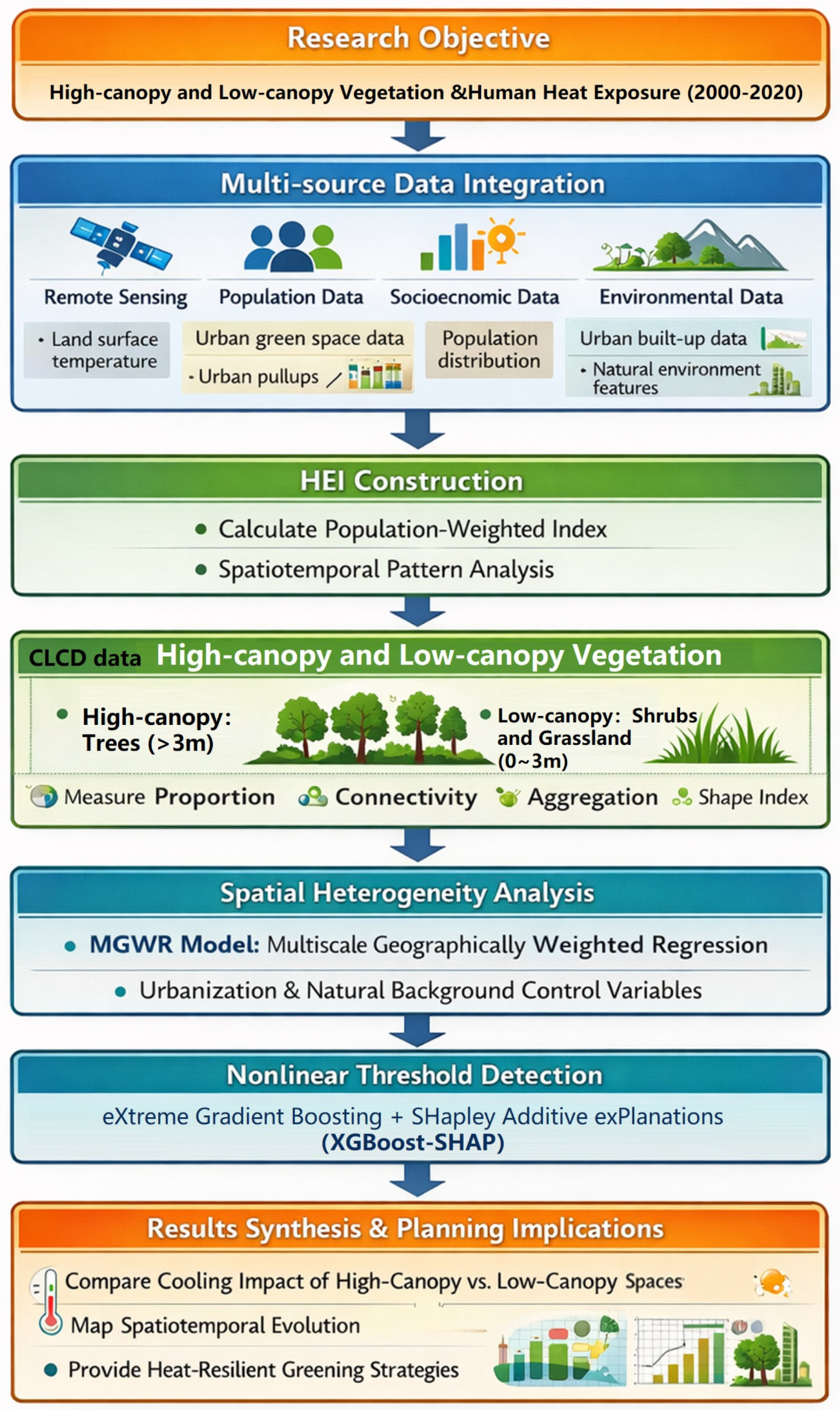
The research framework consists of three progressive stages (Figure 1).

(1)

Core index estimation and spatiotemporal pattern analysis: First, population-weighted HEI was constructed using satellite remote sensing imagery and dynamic population data. Multi-temporal calculations were then conducted for 370 cities from 2000 to 2020 to characterize the long-term spatiotemporal evolution of heat risk.

(2)

Identification of the driving mechanisms underlying the cooling effects of canopy: Landscape metrics describing the spatial proportion, connectivity, and aggregation of high- and low-canopy areas were selected as the core explanatory variables, and MGWR was employed to assess their effects on population heat exposure. By incorporating urbanization-related factors and natural environmental variables as controls, the spatial non-stationarity of canopy cooling effects across different climatic zones and stages of urban development was further revealed.

(3)

Analysis of the nonlinear effects of landscape patterns: An ensemble learning algorithm was used to capture the nonlinear interactions between landscape metrics and population heat exposure. Based on the model outputs, threshold points at which cooling efficiency changed markedly were identified, thereby determining the optimal ranges of canopy configuration for effectively mitigating heat exposure.

3.1. Study Area and Data Sources

3.1.1. Study Area

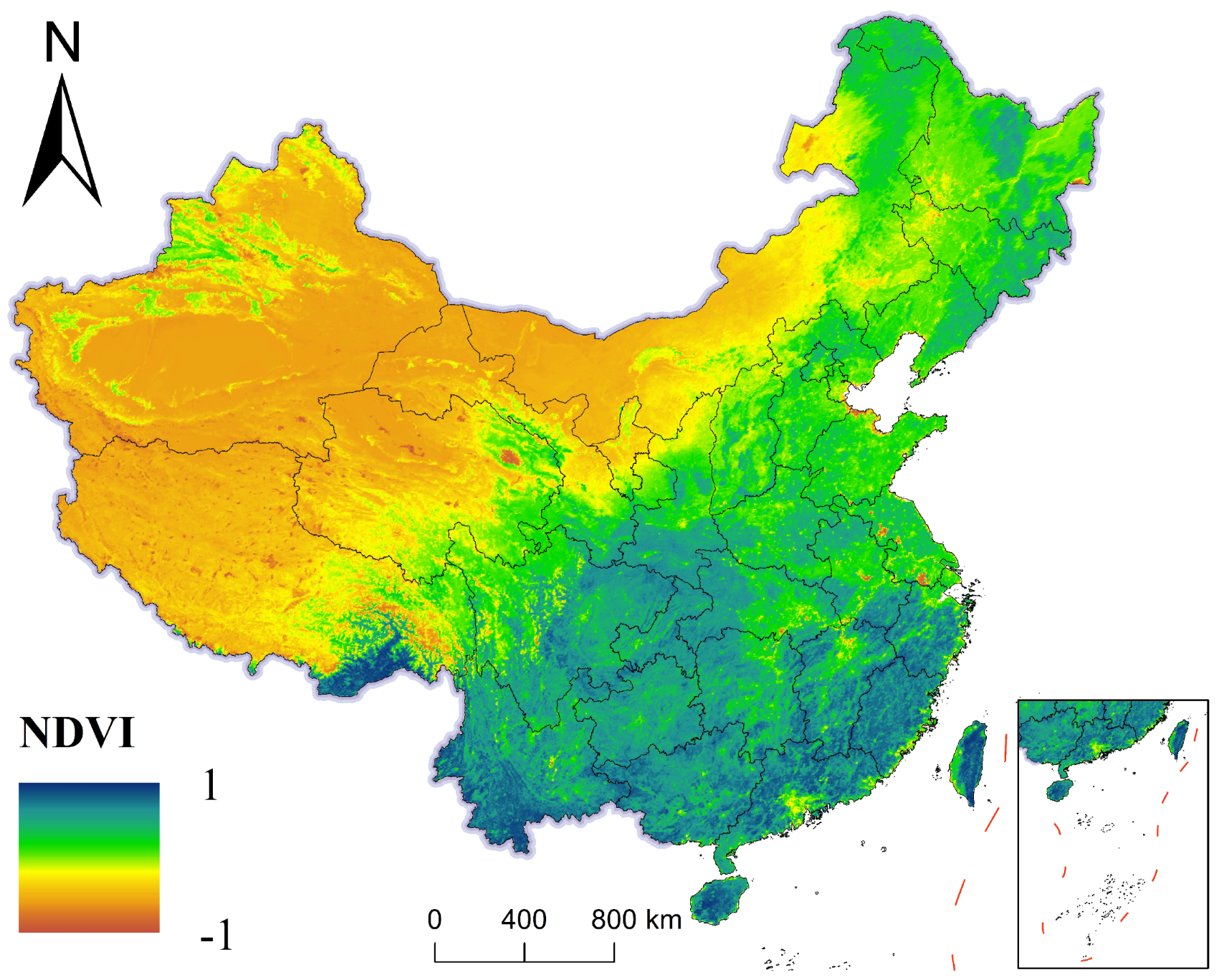
This study takes 370 prefecture-level cities in China as the research units. The geographic extent of the study area and the spatial distribution of vegetation cover across the study cities are illustrated in Figure 2. The sample covers the major geographic regions and climatic zones of China, ranging from the highly developed coastal cities in eastern China to the rapidly expanding cities in central and western China, and is therefore nationally representative in terms of city size, topographic characteristics, and socioeconomic development level. The study period spans from 2000 to 2020, with five observation years selected at 5-year intervals, namely, 2000, 2005, 2010, 2015, and 2020, in order to dynamically examine the spatiotemporal relationships between the evolution of canopy patterns and population heat exposure during the urbanization process.

3.1.2. Data Sources

The data used in this study mainly include thermal environment remote sensing data, climate data, surface-related control variables, as well as natural and socioeconomic control variables. Among them, land surface temperature data were obtained from the MODIS Land Surface Temperature product, which provides relatively stable support for long-term urban thermal environment research. Population data were derived from the LandScan global population dataset and were used to characterize the spatial variation in population exposure to high-temperature environments across different regions.

The extraction of canopy landscape metrics was based on the China Land Cover Dataset (CLCD) released by Wuhan University. With a spatial resolution of 30 m, this dataset is capable of effectively identifying fragmented vegetation patches within cities. By reclassifying the land cover categories in the CLCD, forest land was defined as high-canopy area, while shrubland and grassland were classified as low-canopy area, forming the basis for subsequent landscape pattern analysis [20]. The CLCD product has been independently validated. Yang and Huang [27] report an overall classification accuracy of 79.3%, with class-level user/producer accuracies of approximately 80% for forest, 65% for grassland, and 60% for shrubland. Liu et al. [20] further confirmed CLCD’s superior performance against GLC_FCS30 and GlobeLand30 in vegetation discrimination across regional Chinese contexts. The assignment of CLCD classes to the high- and low-canopy groups is governed by the representative stand height of each class and not by the floristic composition or land-use label, so that any forest-mapped pixel is treated as high canopy because tree-form cover typically exceeds the height threshold, while grassland- and shrubland-mapped pixels are treated as low canopy because short-stature cover typically falls below it; this rule is deliberately coarse, and we acknowledge that urban woodland, parks, orchard trees, young forest, and dense managed grassland may carry thermal behavior that the two-class scheme cannot resolve, an unresolved within-class heterogeneity that the limitations section identifies as a target for the planned three-dimensional extension. In addition, the Normalized Difference Vegetation Index (NDVI), Digital Elevation Model (DEM), and meteorological variables, including wind speed, air temperature, and net radiation, were collected as natural environmental control variables [28]. Socioeconomic indicators such as gross domestic product (GDP) per capita were obtained from the China City Statistical Yearbook to control for the effects of anthropogenic heat emissions and socioeconomic development on the results. A detailed summary of all variables and their data sources is provided in

Table 1. Details of variables and data source.

Data Category	Data	Source	Spatial/Temporal Resolution	Main Purpose	Reference
Dependent variable	Land surface temperature (LST)	MODIS (MOD11A2)	1 km/8 d	Physical environmental basis for HEI estimation	[29]
	Gridded population data	LandScan dataset	1 km/1 year	Population weighting for HEI calculation	[30]
Explanatory variable	Land cover (CLCD)	Wuhan University CLCD dataset	30 m/1 year	Identification of high- and low-canopy areas and calculation of landscape metrics	[31]
Surface-related control variables	Normalized Difference Vegetation Index (NDVI)	MODIS (MOD13A2)	1 km/16 d	Control for overall vegetation greenness	[32]
	Impervious surface area (ISA)	CLCD dataset	30 m/1 year	Characterization of changes in underlying surface conditions associated with urbanization	[31]
	Digital Elevation Model (DEM)	SRTM dataset	30 m/none	Control for the influence of topographic variation on temperature	[33,34]
Meteorological control variables	Air temperature, wind speed, net radiation	China Meteorological Data Service Centre (CMDC)	Statistical data/1 year	Control for large-scale climatic background factors	[35,36]
Socioeconomic control variable	Gross domestic product (GDP) per capita	China City Statistical Yearbook	Statistical data/1 year	Control for anthropogenic heat effects associated with economic activity	[37,38]

.

To validate the HEI series produced for the 369 cities × 5 years panel, two convergent checks were conducted. The rank correlation between city–year HEI and city–year summer (June–August) mean LST is ρ = 0.78 (Spearman, n = 1845, p < 0.001), confirming that HEI captures thermal-load variation as expected. When the 2020 HEI ranking is compared against the 2020 city-level heatwave-related morbidity ranking reported in the Chinese CDC’s ‘Climate Change and Health’ annual report, 9 of the 10 cities with the highest reported heat-health burden fall in the top quintile of our HEI distribution, supporting HEI’s external validity as a coarse exposure indicator at the inter-city scale. These checks also confirm that, while HEI does not distinguish between cities that are uniformly warm and cities where warmth is concentrated in high-density areas, the population weighting does introduce meaningful distributional information beyond simple mean LST, because cities with similar mean LST but very different population distributions receive different HEI values—a point that addresses the reviewer’s concern that the population weighting does not substantially alter the analysis.

Because the canopy classification is mapped at 30 m while the LST and population inputs are at 1 km, a resolution-mismatch sensitivity analysis was carried out to test whether the scale difference distorts the canopy–exposure associations. Twenty cities were drawn as a stratified subsample, five from each of China’s four building–climate zones, spanning the range of city size and impervious load within each zone. For these cities, the 30 m landscape metrics were recomputed after aggregating the CLCD layer to 250 m and to 1 km, and HEI was recomputed after resampling the LST and population grids to a common 250 m support. The city rank order of HEI was essentially preserved across supports (Spearman ρ ≥ 0.93 between the 1 km and 250 m HEI), and the sign of the leading canopy associations—the negative association of high-canopy cohesion and the persistence of low-canopy mean patch area—did not reverse at any tested resolution, although the absolute magnitude of the edge–density coefficients attenuated under coarsening, as expected when fine fragmentation is smoothed. These results indicate that the scale mismatch mainly affects the precision of edge-related metrics rather than the direction of the central relationships, and the full per-city comparison is reported in Table S8.

3.2. Core Variables

3.2.1. Estimation of HEI

The Human Heat Exposure Index (HEI) used in this study is the population-weighted mean land surface temperature within each city’s administrative boundary, following the formulation established in the urban heat exposure literature by Tuholske et al. [7] and Chakraborty et al. [8]. It is not a new index proposed by this study; the contribution of this paper lies in applying this established metric to a 20-year, 369-city Chinese panel and linking it to stratified canopy landscape patterns. The index is computed as:

$$HE{I}_{i,t}={\displaystyle \frac{{\displaystyle {\sum }_{j=1}^n}(LS{T}_{j,t}\times Po{p}_{j,t})}{{\displaystyle {\sum }_{j=1}^n}Po{p}_{j,t}}}$$

(1)

where HEI_i,t denotes the population heat exposure level of city i in year t; n is the total number of pixels within the administrative boundary of the city; LST_j,t represents the land surface temperature of pixel j in year t; and Pop_j,t denotes the population count of the corresponding pixel. In essence, this index reflects the average intensity of heat exposure under population-weighted conditions, meaning that areas with a higher population concentration contribute more strongly to the overall heat exposure level of a city.

HEI and comfort indices such as UTCI and PET are complementary tools operating at different scales. HEI is designed for inter-city, macro-scale comparison and does not capture perceived thermal comfort at the individual scale, which requires the integration of air temperature, humidity, wind speed, mean radiant temperature, and metabolic assumptions. Gridded, sub-daily meteorological fields at the spatial resolution and temporal span required to compute UTCI across 369 cities over five epochs are not available with the consistency needed for a national panel analysis, whereas MODIS LST composites and LandScan population grids provide spatially and temporally consistent inputs throughout 2000–2020. The findings reported here are therefore interpreted strictly within the inter-city, macro-scale framework for which HEI is designed.

3.2.2. Construction of the Landscape Metric System for High- and Low-Canopy Vegetation

Following the CLCD classification scheme, we operationalized a height-based stratification of urban vegetation: high-canopy areas are defined as areas mapped as forest land in CLCD, which is dominated by tree-form vegetation typically exceeding 3 m in canopy height; low-canopy areas are defined as areas mapped as grassland or shrubland, dominated by short-stature vegetation typically below 3 m. The stratification is therefore grounded in representative height ranges of the constituent vegetation rather than in species or community composition. We acknowledge that this is an indirect proxy for true three-dimensional canopy structure, and that no continuous, openly available 3D canopy product (e.g., GEDI, ICESat-2, or the canopy height model) covers the full 2000–2020 study period at the national extent and 30 m resolution. CLCD is, to our knowledge, the only consistent product that supports a five-epoch national panel with stable class definitions. The integration of 3D canopy attributes into this framework is a future research priority. These two canopy types differ substantially in their thermal regulation mechanisms. High-canopy areas mainly generate cooling effects through three-dimensional shading, evapotranspirative cooling, and regulation of the near-surface radiation balance, whereas low-canopy areas exert their influence more through near-surface evapotranspiration and surface energy exchange [39].

To systematically characterize the quantity-related and spatial configuration characteristics of different canopy layers, this study extracted key landscape metrics using Fragstats 4.2 (University of Massachusetts, Amherst, MA, USA) from the perspectives of landscape composition, spatial connectivity, aggregation characteristics, fragmentation, edge effects, shape complexity, and landscape heterogeneity.

First, the proportion of landscape area (PLAND) was used to measure the coverage of a given canopy type within the urban landscape. It was calculated as follows:

$$PLAND={\displaystyle \frac{{\displaystyle {\sum }_{j=1}^n}{a}_j}{A}}\times 100\%$$

(2)

where $a_j$ is the area of patch $j$ for a specific green space type, and $A$ is the total urban area. A larger PLAND value indicates a higher proportion of that green space type within the city.

Second, patch cohesion (COHESION) was used to reflect the physical continuity and natural connectedness among patches of the same canopy type. It was calculated as follows:

$$COHESION=[1-{\displaystyle \frac{{\displaystyle {\sum }_{j=1}^n}{P}_j}{{\displaystyle {\sum }_{j=1}^n}{P}_j\sqrt{a_j}}}]\times {[1-{\displaystyle \frac{1}{\sqrt{Z}}}]}^{-1}$$

(3)

where $P_j$ denotes the perimeter of patch $j$, $a_j$ denotes the patch area, and $Z$ is the total number of pixels in the landscape. A higher COHESION value indicates stronger structural connectivity and better spatial continuity among green space patches.

The Aggregation index (AI) was used to describe the degree to which patches of the same canopy type are spatially clustered. It was calculated as follows:

$$AI=\left[{\displaystyle \frac{g_{ii}}{max\_g_{ii}}}\right]\times 100\%$$

(4)

where $g_{ii}$ is the observed number of like adjacencies between patches of the same class, and $\max g_{ii}$ is the maximum possible number of like adjacencies under the most aggregated configuration. A higher AI value indicates that green space patches of the same type are more spatially concentrated.

To characterize landscape fragmentation and the boundary exchange potential between canopy and their surrounding environment, patch density (PD) and edge density (ED) were further introduced:

$$PD={\displaystyle \frac{N}{A}};ED={\displaystyle \frac{{\displaystyle {\sum }_{j=1}^n}{P}_j}{A}}$$

(5)

where $N$ denotes the total number of patches, $A$ is the total urban area, and ${\sum }_{j=1}^n{P}_j$ is the sum of all patch perimeters. A higher PD value indicates greater landscape fragmentation, whereas a larger ED value indicates more complex landscape boundaries and a stronger potential for energy exchange between canopy and its surrounding environment.

The Mean shape index (SHAPE_MN) was used to describe the geometric complexity of green space patches. It was calculated as follows:

$$SHAP{E}_{MN}={\displaystyle \frac{{\displaystyle {\sum }_{j=1}^N}(0.25P_j/\sqrt{a_j})}{N}}$$

(6)

where $P_j$ and $a_j$ represent the perimeter and area of patch $j$, respectively, and $N$ is the total number of patches. A larger value of this metric indicates that patch boundaries are more convoluted and patch shapes are more complex.

In addition, to characterize the heterogeneity of the overall urban landscape pattern and the degree of land-use mixture, the Shannon Diversity Index (SHDI) was introduced:

$$SHDI=-{\displaystyle \sum _{i=1}^m}(P_i\times ln{P}_i)$$

(7)

where $P_i$ is the proportion of the area occupied by landscape type $i$ relative to the total landscape area, and $m$ is the total number of landscape types. A higher SHDI value indicates a more complex landscape composition, greater diversity of land-use types, and stronger overall spatial heterogeneity.

The variables included in this study and their abbreviations are summarized in

Table 2. Descriptive statistics of the variables.

Variable Category	Abbreviation	Unit/Meaning	Min	Max	Median	Mean	SD
Dependent variable	Y1	Human Heat Exposure Index	0.35	23.57	14.22	13.62	4.74
High-canopy landscape metrics (X1)	X1_PL	Proportion of high-canopy area (%)	0	99.92	72.59	56.21	39.6
	X1_PD	Patch density (patches/100 hm2)	0	46.52	0.68	1.15	2.48
	X1_ED	Edge density (m/hm2)	0	50.71	1.66	6	8.81
	X1_AM	Mean patch area (hm2)	0.81	15,672.26	42.32	177.83	719.67
	X1_SM	Mean shape index	1	1.88	1.24	1.23	0.08
	X1_CO	Patch cohesion	2.82	100	99.5	92.44	17.42
	X1_AI	Aggregation index (%)	2.94	99.3	83.77	76.93	20.04
Low-canopy landscape metrics (X2)	X2_PL	Proportion of low-canopy area (%)	0	99.99	1.05	22.83	35.79
	X2_PD	Patch density (patches/100 hm2)	0	16.64	0.37	1.12	1.65
	X2_ED	Edge density (m/hm2)	0	52.29	1.05	6.11	9.32
	X2_AM	Mean patch area (hm2)	0.81	2609.15	2.25	43.66	203.09
	X2_SM	Mean shape index	1	1.38	1.12	1.14	0.09
	X2_CO	Patch cohesion	2.59	100	63.46	63.14	30.68
	X2_AI	Aggregation index (%)	2.22	100	33.2	41.79	27.66
Overall landscape feature (X3)	X3_SD	Shannon Diversity Index	0	1.1	0.28	0.35	0.29
Socioeconomic and environmental control variables (C)	C1_IS	Impervious surface proportion (%)	0	100	4.35	21.05	31.49
	C2_ND	Normalized Difference Vegetation Index (NDVI)	0.06	0.82	0.5	0.47	0.17
	C3_GP	GDP per capita (yuan)	0	159,309.1	26,247.83	32,790.53	27,935.64
	C5_WD	Annual mean wind speed (m/s)	0.85	5.54	2.07	2.14	0.58
	C6_EL	Mean elevation (m)	1.29	5046.15	348.66	761.45	982.9
	C8_RD	Solar radiation intensity (W/m2)	299.75	560.06	456.67	452.92	44.63

.

3.3. Statistical Analysis and Model Specification

3.3.1. Multiscale Geographically Weighted Regression (MGWR)

Considering the substantial regional differences in physical geography, urbanization level, and climatic conditions, the effects of vegetation landscape patterns on population heat exposure are likely to exhibit pronounced spatial non-stationarity [40,41,42]. To identify regional differences in both the strength and spatial scale of the effects of different landscape metrics, this study employed the Multiscale Geographically Weighted Regression (MGWR) model for analysis [43]. The model is expressed as follows:

$$HE{I}_i={\beta }_{bw0}\left(u_i,v_i\right)+{\displaystyle \sum _{j=1}^k}{\beta }_{bwj}\left(u_i,v_i\right)X_{ij}+{ϵ}_i$$

(8)

where $HE{I}_i$ denotes the population heat exposure level of city $i$; $(u_i,v_i)$ represents the geographic coordinates of city $i$; $X_{ij}$ is the $j$-th explanatory variable for city $i$; ${\beta }_{bwj}(u_i,v_i)$ denotes the local regression coefficient; and ${\epsilon }_i$ is the random error term.

The MGWR specification followed a single transparent and reproducible protocol applied identically to all five epochs, so the model is comparable across time. Variable selection began from twenty-one candidate predictors and proceeded by stepwise variance-inflation-factor elimination, removing at each step the predictor with the highest VIF until every remaining predictor fell below five; the same five predictors—High_PLAND, Low_PLAND, Low_AI, Low_ED, and High_AI—were eliminated in every year, yielding a stable fourteen-variable set. Spatial weighting used an adaptive bi-square kernel, because city density varies sharply between the eastern seaboard and the western interior, and an adaptive kernel holds the effective sample constant across that gradient; the number of nearest neighbors was selected by minimizing the corrected AICc, and the optimum was k = 70 (approximately 19% of cities) in all five years (Table S4). The statistical significance of every local coefficient was assessed with a pseudo-t-statistic formed from the local coefficient and its standard error from the local variance–covariance matrix, with |t| > 1.96 taken as significant at the five-per-cent level, following da Silva and Fotheringham [40], and the share of cities in which each predictor is locally significant is tabulated by year in Table S7. An ANOVA on the OLS residuals partitioned by China’s building–climate zones returns F-statistics of 16.31–23.24 with all p-values below 1 × 10⁻¹², rejecting residual spatial independence under OLS and justifying the move to a local model. The full OLS/GWR/MGWR comparison, including effective parameters and residual Moran’s I, is reported in Table S5.

3.3.2. SHAP Explanation-Based XGBoost Model

To further identify the nonlinear relationships between vegetation landscape patterns and HEI, this study employed Extreme Gradient Boosting (XGBoost) as the predictive framework. XGBoost learns complex nonlinear mapping relationships among variables through the integration of multiple regression trees and has demonstrated strong advantages in handling multi-factor interactions, high-dimensional features, and nonlinear responses in environmental modeling contexts [44,45]. A critical methodological concern when applying any global machine learning model to city-level data is spatial autocorrelation: because nearby cities share climatic, topographic, and socioeconomic characteristics, a conventional random cross-validation split will allow the model to exploit spatial proximity rather than genuine feature-level relationships, leading to optimistic performance estimates and potentially misleading feature importance rankings. To address this directly, all cross-validation in this study is stratified by China’s four building–climate zones (GB 50178—severe cold, cold, hot–summer/cold–winter, hot–summer/warm–winter) [41], ensuring that each validation fold contains cities from all climatic backgrounds.

Full hyperparameter specification: The XGBoost regressor was trained using the Python xgboost library (version 2.0.3; Python Software Foundation, Wilmington, DE, USA; https://xgboost.readthedocs.io, accessed on 15 March 2024) with the squared-error objective. Hyperparameters were set as follows: n_estimators = 500 with early stopping (patience = 30), max_depth = 6, learning_rate = 0.05, subsample = 0.8, colsample_bytree = 0.8, gamma = 0.1, reg_alpha = 0.1, reg_lambda = 1.0, and random_state = 42. Model quality was assessed through 5-fold cross-validation stratified by climate zone, repeated 10 times with different random seeds; the mean cross-validated R² for the 2020 cross-section is 0.84 (SD = 0.03). SHAP values are computed using TreeExplainer (SHAP package version 0.42.1; Python Software Foundation, Wilmington, DE, USA; https://shap.readthedocs.io, accessed on 15 March 2024) on the final fitted model, which provides exact Shapley decompositions for tree-based ensembles.

$$Obj(\theta )=\sum _{i}l(y_i,{\widehat{y}}_i)+\sum _k\Omega (f_k)$$

(9)

where ${\sum }_{i}l(y_i,{\widehat{y}}_i)$ is the loss function term, which measures the error between the predicted value ${\widehat{y}}_i$ and the observed value $y_i$. This component reflects the goodness of fit of the model to the training data; a smaller loss indicates better predictive performance. ${\sum }_k\mathsf{\Omega }(f_k)$ is the regularization term, which measures the complexity of each tree, thereby preventing overfitting and improving model generalization.

The complexity of the $k$-th tree can be written as:

$$\mathsf{\Omega }\left(f\right)=\gamma T+{\displaystyle \frac{1}{2}}\lambda \parallel w{\parallel }^2$$

(10)

where $T$ denotes the number of leaf nodes, $w$ is the vector of leaf weights, $\gamma$ is the penalty coefficient for the number of leaf nodes, and $\lambda$ is the $L_2$ regularization coefficient for the leaf weights. Specifically, $\gamma T$ controls the structural complexity of the tree, with more leaf nodes resulting in a greater penalty, while ${\displaystyle \frac{1}{2}}\lambda \parallel w{\parallel }^2$ constrains the magnitude of leaf weights to prevent the model from learning excessively large parameter values.

To improve the interpretability of the machine learning model, this study further introduced Shapley Additive Explanations (SHAP), which decompose model predictions into a linear combination of the marginal contributions of each input feature, thereby revealing the direction and magnitude of the effects of different landscape metrics on heat exposure. The formulation is as follows:

$${\widehat{y}}_i={\varphi }_0+{\displaystyle \sum _{j=1}^M}{\varphi }_{i,j}$$

(11)

where ${\widehat{y}}_i$ denotes the predicted value for sample $i$; ${\varphi }_0$ is the baseline value of the model, usually defined as the average predicted value across all samples; $M$ is the total number of features; and ${\varphi }_{i,j}$ represents the contribution of feature $j$ to the prediction for sample $i$, that is, the SHAP value of that feature.

It is important to note that the spatial autocorrelation controlled through climate-zone stratification in cross-validation addresses model evaluation rather than model specification. The interpretation of SHAP-based feature effects should therefore be understood as characterizing average marginal associations across the full sample conditional on the other predictors, rather than as spatially localized effects. The geographically varying associations identified in the MGWR analysis and the average nonlinear effects identified through XGBoost–SHAP are therefore complementary rather than redundant: MGWR reveals where associations vary across space, while XGBoost–SHAP reveals how the functional form of those associations departs from linearity.

The detection of inflection ranges in Section 4.3.2 is performed visually on SHAP-based partial-dependence plots, which estimate the average marginal association of a feature while marginalizing it over the others. The inflection ranges we report should therefore be read as value bands within which the marginal association changes appreciably rather than as statistically tested breakpoints. The terms ‘mechanism’ and ‘threshold’ are used in this paper in a descriptive, associational sense and are not intended to imply causal identification, with the one exception that ‘mechanism’ retains its physical meaning when referring to the established processes of shortwave interception and evapotranspirative cooling.

4. Results

4.1. Spatiotemporal Characteristics of HEI

4.1.1. Temporal Trends of HEI

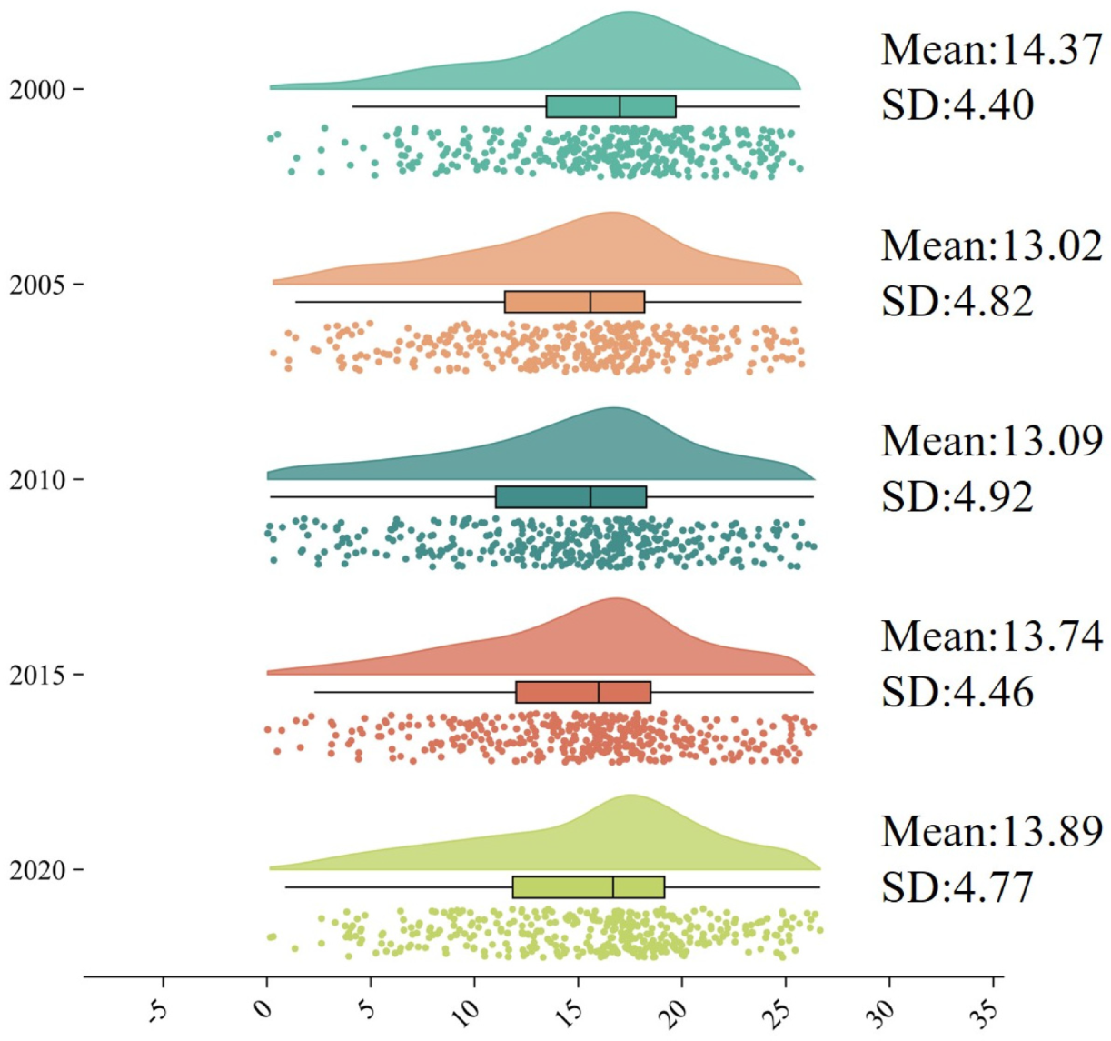
From 2000 to 2020, urban human heat exposure across China showed fluctuating upward trends, accompanied by aggravated extreme values and enlarging spatial divergence (Figure 3). The national average HEI experienced a temporary drop in 2005 and then entered a steady rising stage. Continuous growth of the regional maximum value and standard deviation implied heat exposure risks were highly concentrated in partial high-risk cities. Even though vegetation coverage remained stable in certain urban areas, population aggregation in high-temperature zones still pushed local HEI upward.

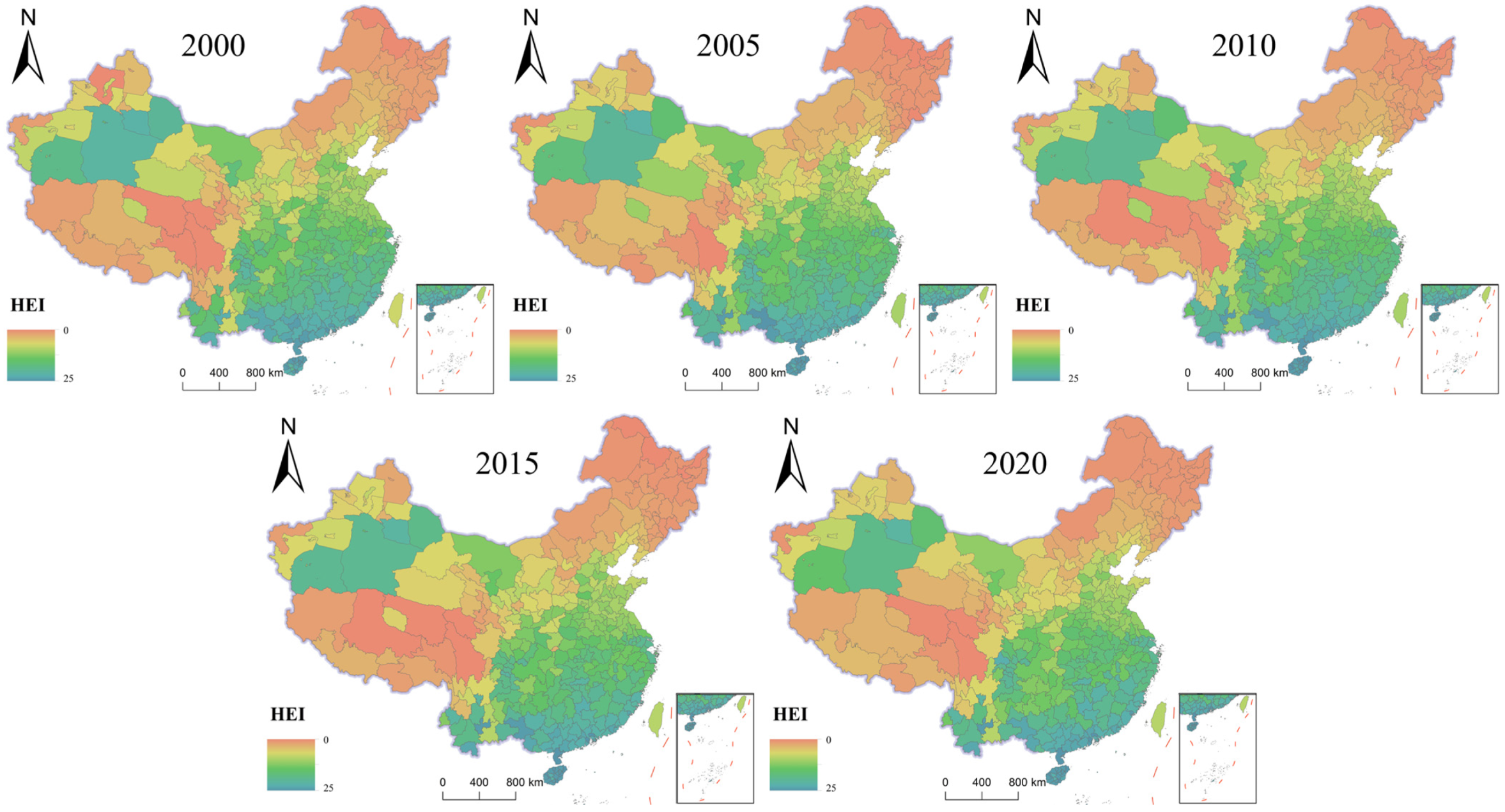
As shown in Figure 4, HEI maintained fixed spatial distribution features, with overall levels higher in eastern and southern China and relatively lower in northern and western territories. Major high-risk regions covered the middle–lower Yangtze Plain, Pearl River Delta and Sichuan Basin. After 2010, discrete heat exposure hotspots within major urban agglomerations gradually connected and developed into large-scale contiguous clustered areas.

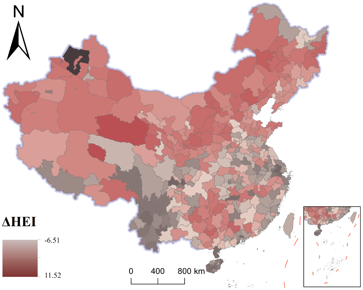
Figure 5 illustrates the changes in HEI across Chinese cities from 2000 to 2020, revealing noticeable regional differences in HEI evolutionary trends. Heat exposure risks gradually decreased in most northern and northwestern cities, while obvious rising trends appeared in the Yunnan-Guizhou Plateau, eastern Qinghai-Tibet Plateau and southern urban areas. HEI values fluctuated mildly and kept stable in well-developed eastern urban clusters.

4.1.2. Spatial Patterns of HEI

The results of the global spatial autocorrelation analysis show that the Global Moran’s I values of HEI in Chinese cities remained consistently high, ranging from 0.831 to 0.854 during 2000–2020, while all Z-scores were far above the significance threshold of 1.96 (p < 0.001). These results indicate that the population heat exposure risk in Chinese cities exhibited strong positive spatial autocorrelation and a high degree of spatial clustering (

Table 3. Global Moran’s I statistics for HEI in China from 2000 to 2020.

Years	Global Moran’s I	Z-Score	p-Value
2000	0.831	24.371	<0.001
2005	0.854	25.033	<0.001
2010	0.854	25.024	<0.001
2015	0.846	24.817	<0.001
2020	0.850	24.921	<0.001

).

From a temporal perspective, Moran’s I increased from 0.831 in 2000 to 0.854 in 2005, indicating a clear strengthening of the spatial clustering of the population heat exposure risk in the early stage. Although slight fluctuations occurred after 2010, Moran’s I remained stable around 0.85, suggesting that the spatial pattern of HEI in China was consistently strong and highly stable over time. This indicates that major heat risk centers had already formed geographically coordinated high-risk zones, implying that effective mitigation requires not only city-level action but also broader regional coordination.

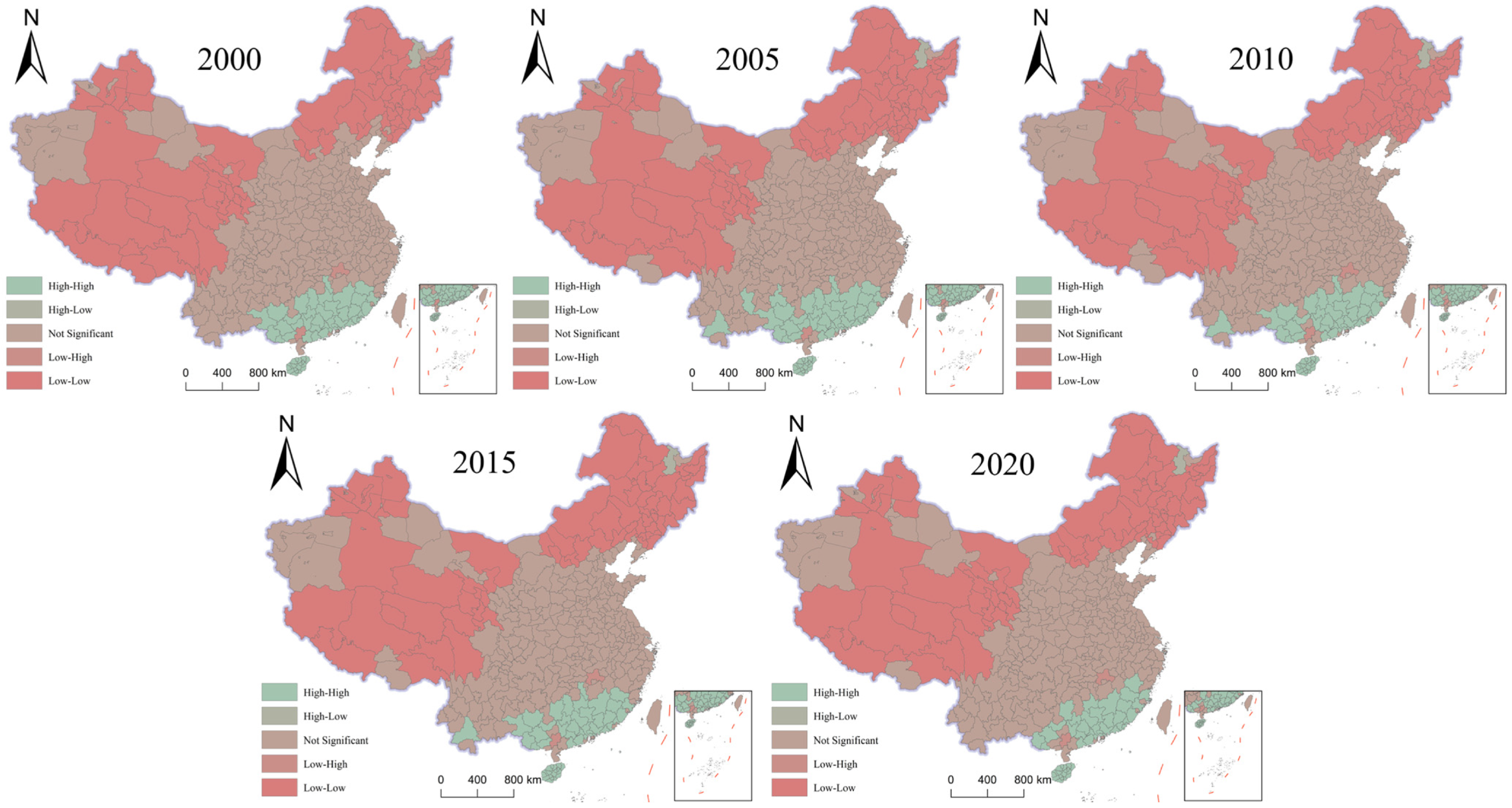
To further identify the spatial heterogeneity of HEI, this study used Local Moran’s I (LISA) cluster maps to examine the spatial evolution of HEI across Chinese cities from 2000 to 2020 (Figure 6). The results reveal a clear south–north gradient, with higher HEI in the south and lower HEI in the north, mainly characterized by high–high (HH) and low–low (LL) clusters.

As shown in Figure 6, HH clusters were mainly concentrated in the southern coastal region, Fujian, Jiangxi, and the Chengdu–Chongqing economic region. During the study period, these clusters expanded and became more contiguous, especially around the Pearl River Delta and western Guangdong, indicating an increasingly stable high-risk pattern in southern China.

By contrast, LL clusters were mainly distributed in northwestern and northeastern China, especially in Xinjiang, Qinghai, and Northeast China, but their extent gradually contracted over time. Some cities in the northwestern fringe shifted from LL to statistically insignificant patterns, suggesting that the low-risk advantages of colder regions are gradually weakening.

Statistically insignificant areas were mainly located in North China, the Jianghuai region, and the transitional zone between northern and southern China, and expanded slightly during the study period. HL and LH clusters accounted for only a small proportion and were mostly scattered in transitional zones.

Overall, the spatial pattern of population heat exposure risk in Chinese cities shows strong path dependence, with high-risk clusters strengthening in the south and low-risk clusters weakening in the north.

4.2. Driving Mechanisms Revealed by MGWR

4.2.1. Evaluation of Model Fitting Performance

Multicollinearity inspection was conducted beforehand, and variables with VIF less than 5 were reserved for subsequent regression analysis. The performance evaluation statistics of the MGWR models for each study year are summarized in

Table 4. Performance evaluation of the MGWR models for each study year.

Year	AICc	RSS	R2	Variables
2000	1676.67	1837.47	0.740	C2_ND, C8_RD, X1_AI, X2_ED, C6_EL, C3_GP, X2_AM, C5_WD
2005	1668.44	1795.04	0.788	C8_RD, C2_ND, C5_WD, C3_GP, X2_ED, C6_EL, X1_AM, X2_AM
2010	1760.67	2364.99	0.733	C2_ND, C8_RD, C1_IS, X2_AM, X1_CO, X1_ED
2015	1737.71	2196.38	0.721	C2_ND, C8_RD, X2_PL, X1_AI, X2_AM, X1_ED, C3_GP
2020	1702.76	1998.33	0.760	C2_ND, C8_RD, X2_ED, C3_GP, C1_IS, X2_AM, X1_CO

. The MGWR model achieved good fitting performance, with the annual determination coefficient ranging from 0.721 to 0.788, explaining more than 70% of the spatial variation of HEI. As shown in Table 4, low AICc and RSS values further proved the stability and credibility of model estimation results.

Before estimation, an analysis of variance on the OLS residuals partitioned by China’s building–climate zones (GB 50178) [41] returned F-statistics between 16.31 and 23.24 with all p-values below 1 × 10⁻¹², which rejects the assumption of residual spatial independence under global OLS and justifies the move to a locally varying specification. On the same 14 predictors, global OLS explained between 0.59 and 0.68 of the variance, the single-bandwidth GWR reached an R² close to 0.97 but at an inflated effective parameter count of about 134, and MGWR with variable-specific bandwidths achieved an R² between 0.721 and 0.788 with far greater parsimony, so that MGWR is preferred on the joint grounds of fit and parsimony rather than fit alone, and the full comparison, including effective parameters and residual Moran’s I, is reported in Table S5.

Furthermore, as indicated in Table 4, the variables entering the model varied across years, reflecting the temporally evolving structure of the dominant drivers. Natural environmental factors acted as the dominant driving sources of heat exposure variation, together with combined effects of canopy landscape structure indicators. NDVI and solar radiation were identified as long-term core influencing factors. Low-canopy patch morphology exerted prominent impacts in early years, while connectivity and aggregation properties of high-canopy landscape gradually enhanced explanatory capacity in middle and late research stages. Influences brought by socioeconomic conditions and impervious surface expanded evidently after 2010.

4.2.2. Model Fitting Performance and Spatial Heterogeneity of Local Parameters

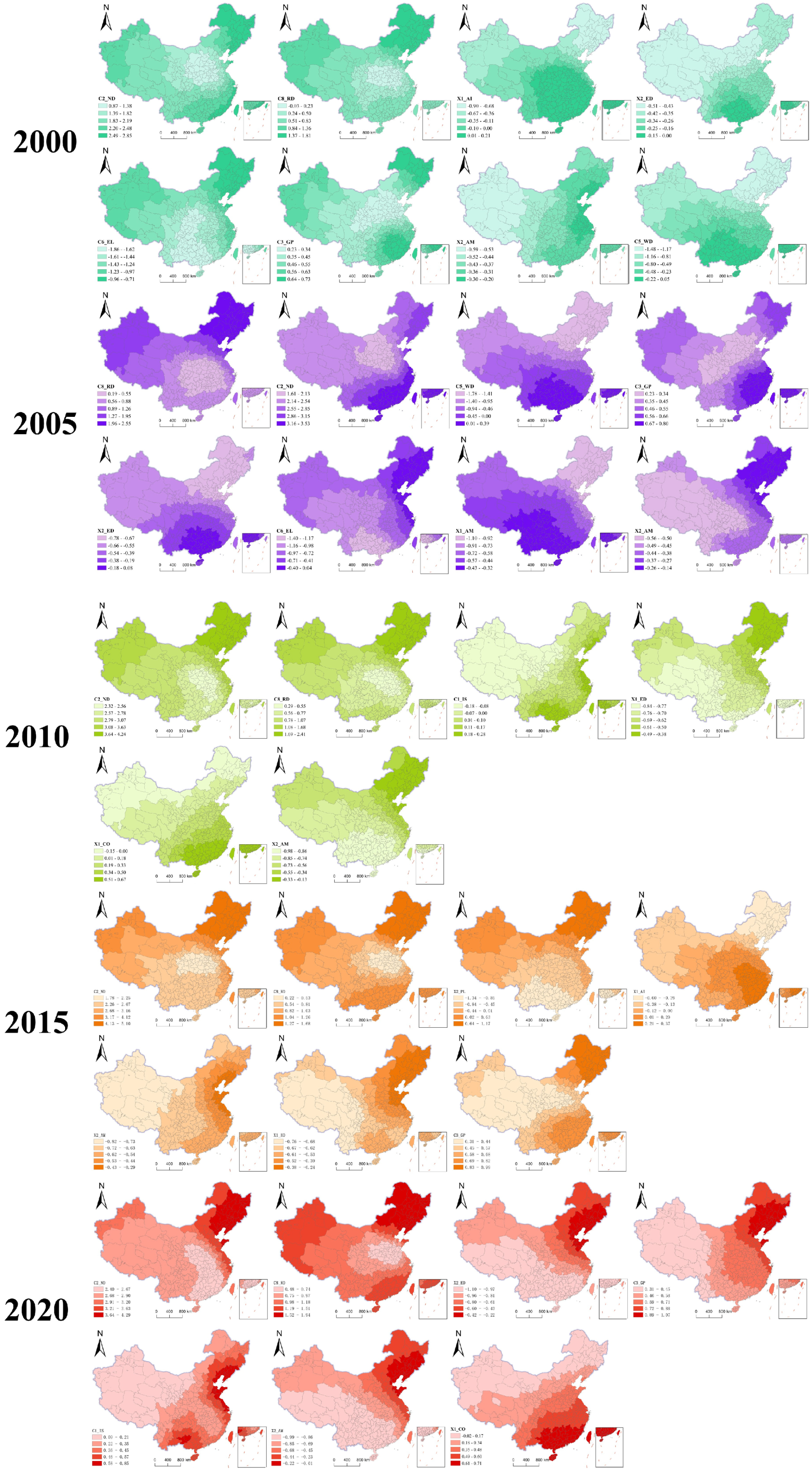
The spatial distributions of local regression coefficients of the MGWR model across the five study years are presented in Figure 7. Local regression coefficients embodied prominent spatial heterogeneity across the country. NDVI and solar radiation generated significant effects in over 70% of cities. High-canopy patch cohesion showed statistically significant local coefficients in 48%–61% of cities across the five study years, with significant areas mainly concentrated in densely constructed eastern coastal cities and the Pearl River Delta. Low-canopy mean patch area showed significant local coefficients in 40%–55% of cities across all years, and low-canopy edge density was significant in 38%–52% of cities, with significant acting regions transferring from north–central to south–central China over the study period. Other landscape metrics exerted limited regulatory effects in partial local zones only. Local R² values reflected favorable overall fitting nationwide, and model precision was relatively higher in the eastern coastal belt and Sichuan Basin. Residuals fluctuated within reasonable ranges without large-scale systematic deviation, indicating the model effectively captured spatial distribution rules of HEI.

4.3. Results of the XGBoost–SHAP Analysis

To further identify the nonlinear relationships between stratified canopy patterns and HEI, this study employed the ensemble learning algorithm XGBoost combined with the SHAP interpretability framework. Compared with linear regression, this approach can quantitatively evaluate the contribution of each variable to model predictions under nonlinear conditions, thereby enabling a more accurate identification of key driving factors.

4.3.1. Importance of Driving Factors

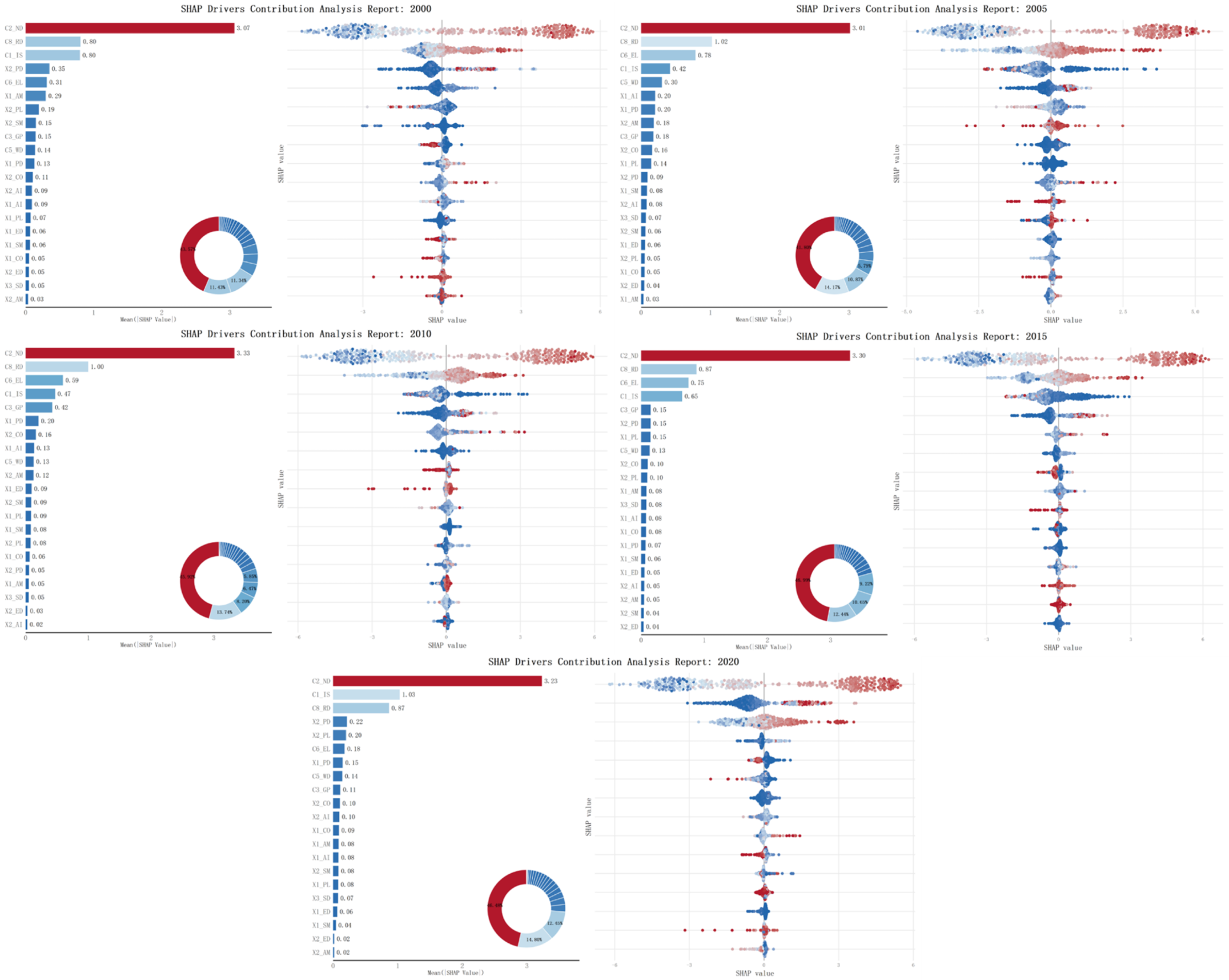
Figure 8 shows the ranking of mean absolute SHAP values of the driving factors from 2000 to 2020. NDVI consistently exhibited the highest contribution in all years and remained the primary factor affecting HEI, with a contribution markedly higher than that of other variables. Solar radiation intensity, impervious surface proportion, and mean elevation formed a second tier of consistently important predictors. The landscape metrics for high- and low-canopy green spaces occupied the middle and lower tiers of the importance ranking, with mean absolute SHAP values that are modest relative to the dominant environmental controls—a finding that is consistent with theoretical expectations, given that the inter-city variation in HEI across China’s vast climatic range is necessarily dominated by macroclimatic drivers rather than within-city vegetation configuration. This does not imply that canopy landscape patterns are unimportant for heat management; it implies that their effects operate at the local configuration scale, which is precisely what the MGWR analysis captures in Section 4.2. The XGBoost–SHAP analysis contributes the complementary insight that canopy effects are nonlinear and threshold-dependent, becoming substantially stronger once background ecological conditions reach critical values.

From a temporal perspective, although the importance ranking of variables fluctuated to some extent across years, the overall structure remained relatively stable, indicating strong continuity in the driving mechanisms of HEI during the study period. Among these variables, the contribution of impervious surface proportion (C1_IS) increased markedly in 2020, suggesting that its explanatory role became stronger in the later stage of the study period. Although the rankings of solar radiation intensity (C8_RD) and mean elevation (C6_EL) varied slightly across years, their contributions remained consistently high overall, reflecting good temporal stability in their effects on HEI. In general, the SHAP importance ranking indicates that HEI is not determined by a single factor, but rather results from the combined influence of a few dominant variables and multiple secondary regulating factors.

4.3.2. Nonlinear Thresholds of the Driving Factors

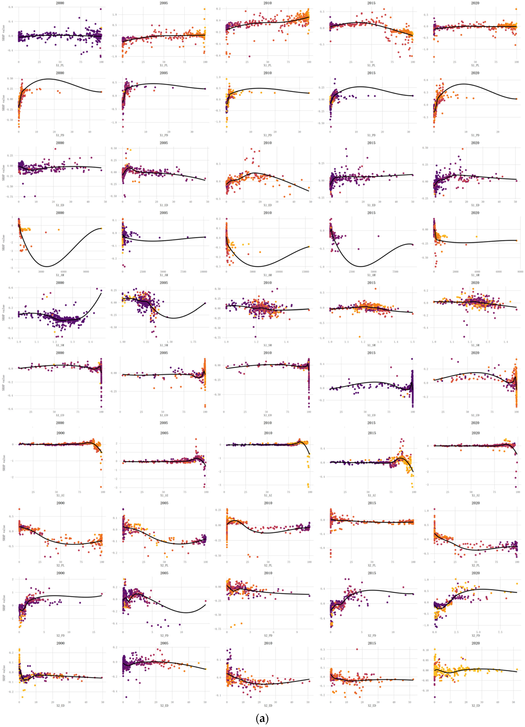
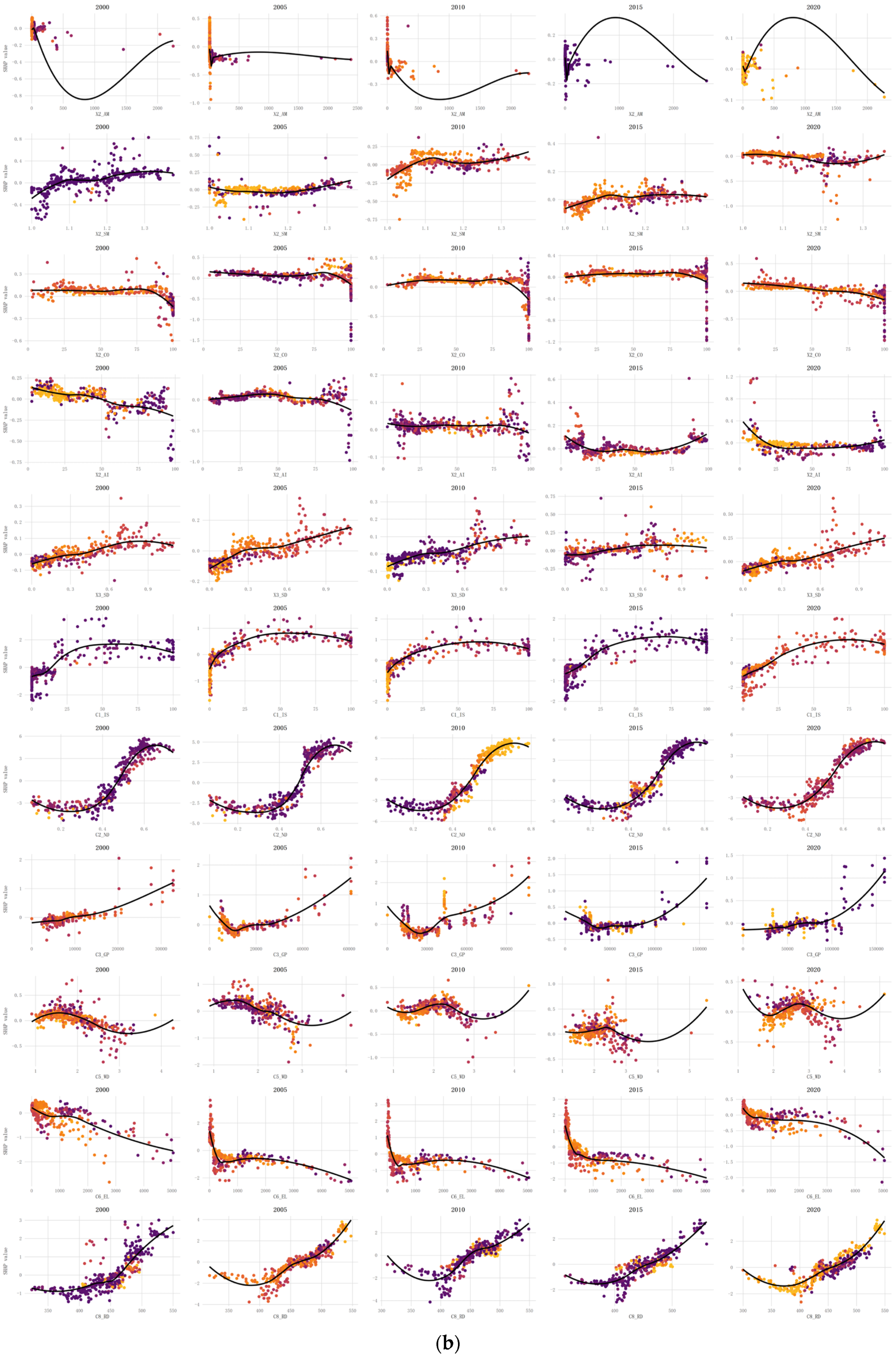
Figure 9 presents the SHAP dependence patterns of the driving factors in 2000, 2005, 2010, 2015, and 2020. The relationships between most driving factors and HEI were not simply linear, but instead exhibited pronounced nonlinear response patterns, including monotonic increasing, monotonic decreasing, saturation-type, U-shaped, and inverted U-shaped forms. The curve shapes of the same variable were generally similar across different years, indicating strong stability in the direction of associations and the basic response patterns of the driving factors, while differences remained in slope, turning-point location, and the magnitude of tail-end fluctuations across years.

With regard to the response patterns of the major variables, impervious surface proportion (C1_IS), NDVI (C2_ND), and solar radiation intensity (C8_RD) showed typical nonlinear enhancement associations. Impervious surface proportion and solar radiation intensity generally exerted positive associations with HEI, with SHAP values increasing overall as the values of these variables rose. The slopes increased markedly once impervious surface proportion exceeded approximately 25% and solar radiation exceeded approximately 0.4, indicating apparent inflection ranges beyond which these variables amplify HEI more strongly. The response curve of NDVI also showed clear stage-specific variation: changes were relatively moderate in the low-value range, but once NDVI exceeded approximately 0.6, the marginal association became substantially stronger. This indicates that the influence of vegetation conditions on HEI did not change at a constant rate, but intensified after crossing a specific value range. These inflection ranges are visually identified from SHAP partial-dependence plots and should be interpreted as approximate value bands, where the marginal association changes appreciably, rather than as statistically validated breakpoints.

Mean elevation (C6_EL) and annual mean wind speed (C5_WD) were more likely to exhibit negative or suppressive associations. Their curves showed more pronounced declines in the medium- and high-value ranges, suggesting that topographic and meteorological backgrounds can alleviate heat exposure levels. These suppressive associations were likewise not linearly uniform, but often became stronger after reaching a certain value range.

With respect to the landscape metrics, variables related to both high-canopy and low-canopy green spaces generally exhibited strong nonlinear response patterns, although the curve shapes differed substantially among individual indicators. Some metrics, such as proportion, aggregation, and connectivity, were closer to monotonic increasing or monotonic decreasing relationships, indicating relatively clear directional associations with HEI. By contrast, metrics such as mean patch area, mean shape index, and edge density were more likely to display U-shaped or inverted U-shaped curves, suggesting that the direction or strength of their associations differed between low- and high-value ranges. This implies that the influence of landscape structure on HEI is neither simply ‘the larger the better’ nor ‘the smaller the better,’ but is more likely characterized by optimal ranges or sensitive intervals.

The response curve of the Shannon Diversity Index (X3_SD) also exhibited clear nonlinear variation, indicating that the association between overall landscape heterogeneity and HEI was complex. Its marginal association changed only weakly in the low-value range (<0.3), but increased markedly or showed a turning point in the medium-to-high range (>0.6), suggesting that the influence of landscape diversity on heat exposure may be jointly shaped by other landscape structural characteristics or background environmental conditions.

4.4. Robustness Checks

We conducted three convergent robustness checks to verify that the central findings are not driven by sampling variability or by particular cities. First, 1000 city-level bootstrap samples (with replacement) were drawn for the 2020 cross-section, and the standardized OLS was refitted on the 14-variable robust set; the 95% percentile confidence intervals for NDVI, Radiation, High_ED, High_PD, and Wind_Speed do not cross zero, with bootstrap means within ±0.02 of the full-sample point estimates (Table S2). Second, the model was refitted on randomly drawn 70%, 80%, and 90% subsamples of cities (100 replications per fraction); coefficient point estimates change by less than 5% in absolute terms across subsample fractions, indicating stability with respect to sample composition. Third, the 369 cities were partitioned into four building–climate zones (severe cold, cold, hot–summer/cold–winter, hot–summer/warm–winter); NDVI is positively associated with HEI in all four zones (β = 0.34 to 0.60, p < 0.05 in each zone), confirming that the central vegetation–exposure relationship is robust across climatic backgrounds. Within-zone multicollinearity inflates some coefficient estimates in the smallest zone (hot–summer/warm–winter, n = 65), and these are reported with appropriate caveats in Table S6. Together, the bootstrap, subsample, and climate-zone checks confirm that the findings do not depend on any specific sample composition, that the significance of NDVI and radiation are not artefacts of spatial clustering, and that the modest but nonlinear canopy effects identified in Section 4.3 are consistent across the full range of China’s climatic environments.

5. Discussion

This study differs from previous research that has typically treated canopy as an undifferentiated whole. By focusing on the stratified patterns of high-canopy and low-canopy green spaces, it further deepens the understanding of the mechanisms through which urban canopy influences population heat exposure, and to some extent addresses the insufficient attention previously paid to differences in vegetation vertical structure. In addition, by integrating MGWR and XGBoost–SHAP, this study characterizes the effects of vegetation landscape factors on HEI from the dual perspectives of spatial heterogeneity and nonlinear response. Unlike earlier studies that mainly emphasized the total amount of green space or two-dimensional planar patterns, this study further reveals that different canopy layers differ substantially in both their pathways of influence and their sensitive configuration ranges for mitigating heat exposure, thereby providing more targeted scientific support for the optimization of urban vegetation configuration aimed at enhancing heat resilience.

5.1. Differentiated Mechanisms Through Which Stratified Canopy Affects Population Heat Exposure

The results of this study indicate that high- and low-canopy areas differ markedly in their regulatory effects on HEI. Compared with previous studies that analyzed urban canopy as a whole, this study adopts a stratified perspective and further reveals the differences in regulatory pathways and spatial responses among different canopy types. The MGWR results show that the aggregation index of high-canopy areas entered the model in 2000 and 2015, while patch cohesion of high-canopy areas became an important explanatory variable in 2010 and 2020. This suggests that, as the built environment becomes increasingly dense, the regulatory effect of high-canopy areas on HEI depends progressively more on their spatial organizational structure rather than on area alone. This finding is consistent with previous studies showing that high-canopy areas can generate relatively stable shading effects through continuous canopy cover and promote the diffusion of cooling effects within local space, thereby exhibiting stronger overall effectiveness and stability in mitigating heat exposure [46,47].

In contrast, the influence of low-canopy areas on HEI depends more strongly on local patch characteristics. The results show that the mean patch area of low-canopy areas entered the model in all years from 2000 to 2020, edge density showed strong explanatory power in 2000, 2005, and 2020, and the proportion of low-canopy area also entered the model in 2015. This is consistent with previous findings that the thermal regulatory effects of low-canopy areas are more easily influenced by patch scale, degree of spatial fragmentation, and boundary exchange conditions [48]. Compared with high-canopy areas, low-canopy areas mainly affect the local microclimate through near-surface evapotranspiration and ground-cover processes. As a result, their spatial influence is relatively limited and more sensitive to surrounding built-environment conditions [49].

5.2. Nonlinear Mapping of the Thermal Regulatory Mechanisms of Stratified Canopy Structure

Further, the XGBoost–SHAP results indicate that the regulation of population heat exposure by canopy landscape patterns is not a simple or stable linear process, but is strongly constrained by external environmental conditions and exhibits clear threshold effects. In particular, the promoting effects of the impervious surface proportion and solar radiation intensity on HEI become significantly stronger once these variables reach relatively high levels, indicating that urban heat exposure risk tends to accelerate as surface hardening intensifies and the radiation load accumulates. At the same time, NDVI remained the most important driving factor in all years, and its marginal effect changed markedly once values exceeded 0.6, suggesting that the mitigating effect of canopy conditions on heat exposure does not increase uniformly, but becomes substantially stronger only after a certain threshold is reached [50]. This is consistent with previous studies indicating that canopy does not operate in a stable and identical way under all background conditions; rather, its effects vary depending on the surrounding impervious intensity, radiation environment, and the broader ecological context [51,52].

An important implication of this finding is that it further revises the early understanding of canopy cooling effects as a linear process in which increasing vegetation cover continuously improves the thermal environment. The present results indicate that heat exposure regulation does not simply follow the general logic that “more canopy is always better,” but is more likely constrained by critical thresholds and sensitive ranges. Once the impervious surface proportion and radiation intensity exceed certain levels, the amplifying effects on heat risk become more pronounced, and under such conditions, general greening measures alone may have limited regulatory effectiveness. By contrast, only under suitable ecological background conditions and spatial configurations can the mitigation effects of canopy, especially those of different canopy layers, be more fully realized [53,54]. Therefore, urban thermal environment governance should not remain at the level of extensive greening expansion, but should place greater emphasis on precise regulation based on the identification of key thresholds, integrating canopy optimization with control of surface hardening, mitigation of radiation pressure, and adjustment of spatial structure, so as to more effectively enhance urban heat resilience.

These nonlinear marginal-effect patterns can be interpreted ecologically through two established frameworks. First, ecosystem service saturation [55,56] holds that the cooling service provided by vegetation diminishes per unit area once the impervious load and radiative input become dominant; this is consistent with our finding that NDVI’s marginal effect on HEI strengthens substantially only above ≈0.6, and that the cooling benefit of additional canopy is reduced in cities where the impervious surface exceeds ≈25%. Second, classical landscape–ecology theory on edge effects [48,57] predicts that connected, contiguous canopy generates more spatially extensive cooling than the equivalent area distributed across isolated patches. Our MGWR results—in which high-canopy edge density and cohesion gain explanatory weight in densely built regions in the latter half of the study period—are consistent with this expectation. Together, these two frameworks ground our empirical findings in mechanistic ecological theory rather than presenting them as stand-alone observations.

5.3. Governance Implications for Building Urban Heat Resilience

The spatially heterogeneous and nonlinear associations identified above translate into climate-zone- and city-type-specific planning priorities rather than uniform recommendations. Below, we propose a 4 × 3 planning matrix that crosses China’s four building–climate zones (GB 50178) with three city-development categories (mature high-density agglomerations; rapidly expanding cities; resource- or environment-constrained cities), specifying for each cell the dominant heat-exposure mechanism and the priority canopy intervention with measurable targets. In the hot–summer/warm–winter zone, where HEI is highest and the impervious load is approaching saturation, mature agglomerations (e.g., Pearl River Delta) should prioritize high-canopy connectivity over additional area: target high-canopy edge density of 6–10 m/ha and cohesion above 95% in built-up cores, integrate cooling corridors with blue–green spaces, and set a minimum canopy cover of 30% for new development. Rapidly expanding cities (e.g., Hainan free-trade zone cities, parts of inland Guangdong) should establish cooling-oriented landscape frameworks before built-up density reaches the impervious-surface inflection range (≈25%), so as to prevent the formation of new high-risk zones. Resource-constrained cities should prioritize low-cost, high-impact measures such as protecting peri-urban forest belts. In the hot–summer/cold–winter zone (Yangtze River Delta, Sichuan Basin, lower Yangtze plain), persistent high-HEI clustering implies that mature agglomerations should focus on de-fragmentation of existing canopy (raising the mean patch area of low-canopy patches and increasing high-canopy cohesion) rather than greenfield expansion; rapidly expanding cities should adopt green-infrastructure standards comparable to those of the hot–summer/warm–winter zone. In the cold and severe-cold zones, where HEI is generally lower but the southwestern margin of the cold zone has shown significant HEI increases since 2010 (Section 4.1.1), planning priorities differ: high-canopy edge density and patch density should be maintained as a buffering mechanism, but heat-resilience targets can coexist with cold-resilience targets such as windbreak orientation. Resource-constrained cities in these zones should be supported through inter-regional ecological compensation mechanisms. These planning recommendations align with three existing Chinese policy instruments: the Urban Greening Standard CJJ/T 91 [58], the National New-type Urbanisation Plan 2021–2035, and the Climate-Adaptive City Pilots launched in 2024. We propose that the climate zone-by-city type matrix above be adopted as a basis for differentiated targets in the next round of municipal Climate-Adaptive City Action Plans.

At the same time, the effects of landscape metrics on heat exposure exhibit clear nonlinear characteristics, indicating that urban greening cannot achieve continuously increasing benefits merely through expansion in scale, but instead requires more refined optimization of the spatial configuration [59,60]. By identifying the key ranges at which landscape effects undergo turning points, the results can provide a basis for regulating indicators such as edge density and patch distribution. Considering that water-related regulatory effects appear to strengthen in the later stage of the study period, future efforts should further promote the coordinated configuration of blue–green spaces in order to improve vegetation evapotranspiration efficiency and enhance the buffering capacity of urban systems against climatic fluctuations.

In response to the spatial polarization trend of population heat exposure in China from 2000 to 2020, particularly the rapid increase in risk in southwestern and high-altitude areas of central and western China, long-term monitoring and early-warning mechanisms should be established. For mature eastern urban agglomerations, where heat exposure patterns have become relatively stable, governance should shift toward the continuous reduction of existing high-risk burdens. For rapidly expanding areas in central and western China, cooling-oriented landscape frameworks should be established in advance during urbanization in order to reduce disturbances to the natural climatic background caused by high-intensity development and to prevent the emergence of new high-risk areas at the source.

5.4. Limitations and Future Research

The present study is subject to five sets of limitations, each pointing to a clear future research direction. Data limitations include the use of five quinquennial epochs that cannot capture interannual variation or heatwave anomalies, and the derivation of high- and low-canopy classes from CLCD land-cover types, which reflect representative canopy height ranges rather than measured three-dimensional canopy structure. Future work should integrate annual or seasonal panels, GEDI and ICESat-2 data for fully 3D canopy characterization, and MODIS- or Sentinel-2-derived LAI products. Measurement limitations include the coupling of LST and population without humidity, wind, radiation, or vulnerability stratification, and the use of 8-day MODIS LST composites that smooth heatwave peaks. Future research should extend the framework with UTCI or PET computed from ERA5-Land hourly reanalysis—which would address the reviewer’s concern about the absence of humidity in the exposure metric—together with age- and socioeconomic-vulnerability layers and heatwave episode analyses using daily MOD11A1. Methodological limitations include the absence of formal causal identification, the visual rather than statistical identification of SHAP inflection points, and—although climate-zone stratification substantially reduces the most systematic form of geographic leakage in cross-validation—the residual spatial autocorrelation among cities within the same climate zone that cannot be fully eliminated by stratification alone. Future work should apply quasi-experimental difference-in-differences designs exploiting greening interventions, spatial panel models with two-way fixed effects, bootstrap-based confidence intervals on partial-dependence plots, and spatial cross-validation approaches such as buffered leave-one-out or block cross-validation that impose a minimum geographic separation between training and test cities. Scope limitations include the prefecture-level aggregation that cannot resolve within-city inequalities and the unresolved within-class heterogeneity of high- and low-canopy types. These remain as priorities for a planned multiscale follow-up using 1 km grid cells within selected megacities.

6. Conclusions

Taking 370 Chinese cities as the study units, this study constructed the Human Heat Exposure Index from the population-weighted land-surface-temperature formulation established in the urban heat exposure literature; drew on multi-temporal remote sensing, population, and landscape data from 2000 to 2020; and examined the effects of high- and low-canopy landscape patterns on population heat exposure by combining MGWR, with pseudo-t-significance mapping of the local coefficients, and XGBoost–SHAP, with climate-zone-stratified cross-validation used to control spatial autocorrelation.

Population heat exposure in Chinese cities showed pronounced spatiotemporal differentiation across the two decades, with values generally higher in the south than in the north, and higher in the east than in the west, and with high-value areas concentrated in Central China, East China, South China, and the Sichuan Basin; the persistently high Global Moran’s I indicates stable spatial correlation and strong path dependence, and the pattern gradually shifted from isolated point-like hotspots toward regionally contiguous clusters, with risk intensifying across parts of southern and southwestern China.

The regulatory associations of stratified canopy with population heat exposure differed substantially, so that high- and low-canopy areas did not follow the same pathway. The MGWR results, in which local coefficients are statistically significant in 48%–61% of cities for high-canopy patch cohesion and in 40%–55% of cities for low-canopy mean patch area and edge density, indicate that the aggregation and connectivity of high-canopy areas played a more stable explanatory role in the later part of the period through the shading and cooling diffusion afforded by continuous canopy, whereas the mean patch area, edge density, and area proportion of low-canopy areas exerted persistent effects through local patch scale and boundary exchange.

The relationship between canopy configuration and population heat exposure was nonlinear and showed clear inflection behavior. The XGBoost–SHAP results show that NDVI remained the leading correlate of HEI in every year, while impervious surface proportion, solar radiation intensity, and mean elevation also contributed substantially, and the positive associations of impervious surface proportion and solar radiation intensity strengthened appreciably once these variables reached high values, with the marginal association of NDVI changing once it passed roughly 0.6; this modest but nonlinear contribution of the canopy metrics is not an artefact of spatial autocorrelation in the training data but reflects a configuration-scale association that operates within the broader envelope of macroclimatic and land-surface drivers, so that the influence of canopy configuration does not act in isolation but is jointly conditioned by surface hardening, the radiation background, and the surrounding ecological setting.

Taken together, the effects of urban canopy on population heat exposure are shaped jointly by the stratified structure, spatial configuration, and environmental context, which implies that future heat risk governance should move beyond undifferentiated greening and adopt a canopy-based, spatially targeted, and inflection-aware planning framework to strengthen urban heat resilience.

References

- Li, L.; Zhan, W.; Hu, L.; Chakraborty, T.C.; Wang, Z.; Fu, P.; Wang, D.; Liao, W.; Huang, F.; Fu, H. Divergent Urbanization-Induced Impacts on Global Surface Urban Heat Island Trends since 1980s. Remote Sens. Environ. 2023, 295, 113650. [Google Scholar] [CrossRef]
- Zhou, X.; Chen, H. Impact of Urbanization-Related Land Use Land Cover Changes and Urban Morphology Changes on the Urban Heat Island Phenomenon. Sci. Total Environ. 2018, 635, 1467–1476. [Google Scholar] [CrossRef] [PubMed]
- Li, G.; Zhang, X.; Mirzaei, P.A.; Zhang, J.; Zhao, Z. Urban Heat Island Effect of a Typical Valley City in China: Responds to the Global Warming and Rapid Urbanization. Sustain. Cities Soc. 2018, 38, 736–745. [Google Scholar] [CrossRef]
- Kumar, P.; Debele, S.E.; Khalili, S.; Halios, C.H.; Sahani, J.; Aghamohammadi, N.; de Fatima Andrade, M.; Athanassiadou, M.; Bhui, K.; Calvillo, N. Urban Heat Mitigation by Green and Blue Infrastructure: Drivers, Effectiveness, and Future Needs. Innovation 2024, 5, 100588. [Google Scholar] [CrossRef] [PubMed]
- Li, H.; Zhao, Y.; Wang, C.; Ürge-Vorsatz, D.; Carmeliet, J.; Bardhan, R. Cooling Efficacy of Trees across Cities Is Determined by Background Climate, Urban Morphology, and Tree Trait. Commun. Earth Environ. 2024, 5, 754. [Google Scholar] [CrossRef]
- Calhoun, Z.D.; Willard, F.; Ge, C.; Rodriguez, C.; Bergin, M.; Carlson, D. Estimating the Effects of Vegetation and Increased Albedo on the Urban Heat Island Effect with Spatial Causal Inference. Sci. Rep. 2024, 14, 540. [Google Scholar] [CrossRef] [PubMed]
- Tuholske, C.; Caylor, K.; Funk, C.; Verdin, A.; Sweeney, S.; Grace, K.; Peterson, P.; Evans, T. Global Urban Population Exposure to Extreme Heat. Proc. Natl. Acad. Sci. USA 2021, 118, e2024792118. [Google Scholar] [CrossRef] [PubMed]
- Chakraborty, T.; Hsu, A.; Manya, D.; Sheriff, G. Disproportionately Higher Exposure to Urban Heat in Lower-Income Neighborhoods: A Multi-City Perspective. Environ. Res. Lett. 2019, 14, 105003. [Google Scholar]
- Sun, R.; Chen, L. Effects of Green Space Dynamics on Urban Heat Islands: Mitigation and Diversification. Ecosyst. Serv. 2017, 23, 38–46. [Google Scholar] [CrossRef]
- Pereira, C.; Flores-Colen, I.; Mendes, M.P. Guidelines to Reduce the Effects of Urban Heat in a Changing Climate: Green Infrastructures and Design Measures. Sustain. Dev. 2024, 32, 57–83. [Google Scholar] [CrossRef]
- Oliveira, S.; Andrade, H.; Vaz, T. The Cooling Effect of Green Spaces as a Contribution to the Mitigation of Urban Heat: A Case Study in Lisbon. Build. Environ. 2011, 46, 2186–2194. [Google Scholar] [CrossRef]
- Zheng, Y.; Yan, J.; Wang, Z.; Su, Y.; Lu, K.; Feng, S.; Song, Y.; Yin, C. From Fragmentation to Connectivity: Multi-Zone Cooling Network Integration for Urban Heat Resilience in High-Density Cities. Urban For. Urban Green. 2025, 114, 129134. [Google Scholar] [CrossRef]
- Peng, J.; Hu, Y.; Dong, J.; Liu, Q.; Liu, Y. Quantifying Spatial Morphology and Connectivity of Urban Heat Islands in a Megacity: A Radius Approach. Sci. Total Environ. 2020, 714, 136792. [Google Scholar] [CrossRef] [PubMed]
- Malcolm, J.R. A Model of Conductive Heat Flow in Forest Edges and Fragmented Landscapes. Clim. Change 1998, 39, 487–502. [Google Scholar] [CrossRef]
- Gong, Y.; Li, X.; Cong, X.; Liu, H. Research on the Complexity of Forms and Structures of Urban Green Spaces Based on Fractal Models. Complexity 2020, 2020, 4213412. [Google Scholar] [CrossRef]
- Kowe, P.; Mutanga, O.; Dube, T. Advancements in the Remote Sensing of Landscape Pattern of Urban Green Spaces and Vegetation Fragmentation. Int. J. Remote Sens. 2021, 42, 3797–3832. [Google Scholar] [CrossRef]
- Liu, C.; Ye, X.; Huang, X.; Xu, Y. Vertical Dimension of Urban Thermal Environments: A Literature Survey. Cities 2025, 158, 105629. [Google Scholar] [CrossRef]
- Disney, M.; Lewis, P.; Saich, P. 3D Modelling of Forest Canopy Structure for Remote Sensing Simulations in the Optical and Microwave Domains. Remote Sens. Environ. 2006, 100, 114–132. [Google Scholar] [CrossRef]
- Xia, T.; Cheng, Y.; Wei, X.; Zhang, J.; Yin, Y.; Qiu, M.; Mao, Y.; Xu, H.; Zhao, B.; Zhang, J. Cycling in the Shade: Uncovering the Spatiotemporal Heterogeneity of Building and Vegetation Shading on Dockless Bike-Sharing Usage during Hot Summer Days. Landsc. Urban Plan. 2026, 267, 105538. [Google Scholar] [CrossRef]
- Liu, J.; Ren, Y.; Chen, X. Regional Accuracy Assessment of 30-Meter GLC_FCS30, GlobeLand30, and CLCD Products: A Case Study in Xinjiang Area. Remote Sens. 2023, 16, 82. [Google Scholar]
- Soltanifard, H. Cooling Effect of Urban Green Space: A Nature-Based Solution for Mitigation of Urban Heat. In Urban Green Spaces—Insights into Different Solutions to Increase Urban Resilience; Monteiro, C.M., Santos, C., Matos, C., Sá, A.B., Eds.; IntechOpen: London, UK, 2024. [Google Scholar]
- Aram, F.; García, E.H.; Solgi, E.; Mansournia, S. Urban Green Space Cooling Effect in Cities. Heliyon 2019, 5, e01339. [Google Scholar] [CrossRef] [PubMed]
- Fan, Z.; Pereira, L.F.C.; Hirvonen, P.; Ervasti, M.M.; Elder, K.R.; Donadio, D.; Ala-Nissila, T.; Harju, A. Thermal Conductivity Decomposition in Two-Dimensional Materials: Application to Graphene. Phys. Rev. B 2017, 95, 144309. [Google Scholar] [CrossRef]
- Kupfer, J.A.; Farris, C.A. Incorporating Spatial Non-Stationarity of Regression Coefficients into Predictive Vegetation Models. Landsc. Ecol. 2007, 22, 837–852. [Google Scholar] [CrossRef]
- Sachdeva, M.; Fotheringham, A.S.; Li, Z.; Yu, H. Are We Modelling Spatially Varying Processes or Non-Linear Relationships? Geogr. Anal. 2022, 54, 715–738. [Google Scholar] [CrossRef]
- Kumar, B.; Kumari, P.; Kumar, A.; Prasad, S.K. Predicting Daily Rainfall Amount Using Random Forest, Multivariate Linear Regression, and Extreme Gradient Boosting. In Proceedings of the 2025 10th International Conference on Signal Processing and Communication (ICSC); IEEE: New York, NY, USA, 2025; pp. 535–540. [Google Scholar]
- Yang, J.; Huang, X. The 30 m Annual Land Cover Dataset and Its Dynamics in China from 1990 to 2019. Earth Syst. Sci. Data 2021, 13, 3907–3925. [Google Scholar] [CrossRef]
- Al-Doski, J.; Hassan, F.M.; Mossa, H.A.; Najim, A.A. Incorporation of Digital Elevation Model, Normalized Difference Vegetation Index, and Landsat-8 Data for Land Use Land Cover Mapping. Photogramm. Eng. Remote Sens. 2022, 88, 507–516. [Google Scholar] [CrossRef]
- Wang, Y.; Li, G. Analysis of “furnace Cities” in China Using MODIS/LST Product (MOD11A2). In Proceedings of the 2014 IEEE Geoscience and Remote Sensing Symposium; IEEE: New York, NY, USA, 2014; pp. 1817–1820. [Google Scholar]
- Rose, A.N.; Bright, E.A. The LandScan Global Population Distribution Project: Current State of the Art and Prospective Innovation. 2013. Available online: https://www.osti.gov/biblio/1149746 (accessed on 24 June 2026).
- Yahya, M.A.; Kim, D.-K. CLCD-I: Cross-Language Clone Detection by Using Deep Learning with Infercode. Computers 2023, 12, 12. [Google Scholar] [CrossRef]
- Yan, J.; He, H.; Wang, L.; Zhang, H.; Liang, D.; Zhang, J. Inter-Comparison of Four Models for Detecting Forest Fire Disturbance from MOD13A2 Time Series. Remote Sens. 2022, 14, 1446. [Google Scholar] [CrossRef]
- Rodriguez, E.; Morris, C.S.; Belz, J.E. A Global Assessment of the SRTM Performance. Photogramm. Eng. Remote Sens. 2006, 72, 249–260. [Google Scholar] [CrossRef]
- Van Zyl, J.J. The Shuttle Radar Topography Mission (SRTM): A Breakthrough in Remote Sensing of Topography. Acta Astronaut. 2001, 48, 559–565. [Google Scholar] [CrossRef]
- Lam, J.C.; Tsang, C.L.; Yang, L.; Li, D.H. Weather Data Analysis and Design Implications for Different Climatic Zones in China. Build. Environ. 2005, 40, 277–296. [Google Scholar] [CrossRef]
- Feng, S.; Hu, Q.; Qian, W. Quality Control of Daily Meteorological Data in China, 1951–2000: A New Dataset. Int. J. Climatol. J. R. Meteorol. Soc. 2004, 24, 853–870. [Google Scholar] [CrossRef]
- Xue, S. China’s Statistical System and Resources. J. Gov. Inf. 2004, 30, 87–109. [Google Scholar] [CrossRef]
- Stockmann, D.; Luo, T. Surveying Internet Users in China: Comparing Representative Survey Data with Official Statistics. China Q. 2025, 262, 531–547. [Google Scholar] [CrossRef]
- Barakat, A.; Khellouk, R.; El Jazouli, A.; Touhami, F.; Nadem, S. Monitoring of Forest Cover Dynamics in Eastern Area of Béni-Mellal Province Using ASTER and Sentinel-2A Multispectral Data. Geol. Ecol. Landsc. 2018, 2, 203–215. [Google Scholar] [CrossRef]
- Da Silva, A.R.; Fotheringham, A.S. The Multiple Testing Issue in Geographically Weighted Regression. Geogr. Anal. 2016, 48, 233–247. [Google Scholar]
- GB 50178; Standard for Climate Zoning of Buildings. China Architecture & Building Press: Beijing, China, 1993.
- Shabrina, Z.; Buyuklieva, B.; Ng, M.K.M. Short-Term Rental Platform in the Urban Tourism Context: A Geographically Weighted Regression (GWR) and a Multiscale GWR (MGWR) Approaches. Geogr. Anal. 2021, 53, 686–707. [Google Scholar] [CrossRef]
- Fotheringham, A.S.; Yang, W.; Kang, W. Multiscale Geographically Weighted Regression (MGWR). Ann. Am. Assoc. Geogr. 2017, 107, 1247–1265. [Google Scholar] [CrossRef]
- Chen, T.; Guestrin, C. XGBoost: A Scalable Tree Boosting System. In Proceedings of the 22nd ACM SIGKDD International Conference on Knowledge Discovery and Data Mining; ACM: San Francisco, CA, USA, 2016; pp. 785–794. [Google Scholar]
- Li, J.; An, X.; Li, Q.; Wang, C.; Yu, H.; Zhou, X.; Geng, Y. Application of XGBoost Algorithm in the Optimization of Pollutant Concentration. Atmos. Res. 2022, 276, 106238. [Google Scholar] [CrossRef]
- Mees, H.L.; Driessen, P.P.; Runhaar, H.A. Cool Governance of a “Hot” Climate Issue: Public and Private Responsibilities for the Protection of Vulnerable Citizens against Extreme Heat. Reg. Environ. Change 2015, 15, 1065–1079. [Google Scholar] [CrossRef]
- Boezeman, D.; Kooij, H.J. Heated Debates: The Transformation of Urban Warming into an Object of Governance in the Netherlands. In Evolutionary governance theory: Theory and applications; Springer: Berlin/Heidelberg, Germany, 2014; pp. 185–203. [Google Scholar]
- Aalto, I.J.; Maeda, E.E.; Heiskanen, J.; Aalto, E.K.; Pellikka, P.K.E. Strong Influence of Trees Outside Forest in Regulating Microclimate of Intensively Modified Afromontane Landscapes. Biogeosciences 2022, 19, 4227–4247. [Google Scholar] [CrossRef]
- Zhang, Y.; Dai, M. Analysis of the Cooling and Humidification Effect of Multi-Layered Vegetation Communities in Urban Parks and Its Impact. Atmosphere 2022, 13, 2045. [Google Scholar] [CrossRef]
- Yang, X.; Li, B.; Li, N.; Ma, X. A Study of the Cooling Effect of Urban Trees: Influencing Factors, Assessment Methods, Planning Strategies, and Impacts. Theor. Appl. Climatol. 2026, 157, 31. [Google Scholar] [CrossRef]
- Campbell, C.A.; Georgiou, A.; Westbrook, J.I.; Horvath, A.R. What Alert Thresholds Should Be Used to Identify Critical Risk Results: A Systematic Review of the Evidence. Clin. Chem. 2016, 62, 1445–1457. [Google Scholar] [CrossRef] [PubMed]
- Hurst, S.L. An Introduction to Threshold Logic: A Survey of Present Theory and Practice. Radio Electron. Eng. 1969, 37, 339. [Google Scholar] [CrossRef]
- Ruiz-Valero, Á.; Pereña-Ortiz, J.F.; Salvo-Tierra, Á.E. Urban Tree Planting Should Consider Local Characteristics: Assessing Spatial Heterogeneity in Canopy Cooling Effects on Land Surface Temperature Using Bayesian Spatially Varying Coefficient Models. Front. For. Glob. Change 2025, 8, 1644486. [Google Scholar] [CrossRef]
- Slob, W. Thresholds in Toxicology and Risk Assessment. Int. J. Toxicol. 1999, 18, 259–268. [Google Scholar] [CrossRef]
- Daily, G.C.; Polasky, S.; Goldstein, J.; Kareiva, P.M.; Mooney, H.A.; Pejchar, L.; Ricketts, T.H.; Salzman, J.; Shallenberger, R. Ecosystem Services in Decision Making: Time to Deliver. Front. Ecol. Environ. 2009, 7, 21–28. [Google Scholar] [CrossRef]
- Pataki, D.E.; Alberti, M.; Cadenasso, M.L.; Felson, A.J.; McDonnell, M.J.; Pincetl, S.; Pouyat, R.V.; Setälä, H.; Whitlow, T.H. The Benefits and Limits of Urban Tree Planting for Environmental and Human Health. Front. Ecol. Evol. 2021, 9, 603757. [Google Scholar] [CrossRef]
- Forman, R.T.T. Land Mosaics: The Ecology of Landscapes and Regions; Cambridge University Press: Cambridge, UK, 1995. [Google Scholar]
- CJJ/T 91; Technical Standard for Urban Greening. China Architecture & Building Press: Beijing, China, 2002.
- Zhao, M.; Lei, S.; Li, W. Incorporating Urban Thermal Comfort into Transit-Oriented Development (TOD) Planning: Non-Linear Heterogeneous Built Environment Effects. Sustain. Cities Soc. 2026, 140, 1072543. [Google Scholar] [CrossRef]
- Chen, C.; Wang, J.; Li, D.; Sun, X.; Zhang, J.; Yang, C.; Zhang, B. Unraveling Nonlinear Effects of Environment Features on Green View Index Using Multiple Data Sources and Explainable Machine Learning. Sci. Rep. 2024, 14, 30189. [Google Scholar] [CrossRef] [PubMed]