Article

Do Set-Asides Increase Plantation Establishment? The Case of U.S. Federal Timber Restrictions and Softwood Planting


1
National Academy of Financial and Economic Strategy, Central University of Finance and Economics, Haidian, Beijing 100081, China
2
Department of Agricultural, Environmental and Development Economics, The Ohio State University, Columbus, OH 43210, USA
3
Department of Forestry and Environmental Resources, North Carolina State University, Raleigh, NC 27695, USA
*
Author to whom correspondence should be addressed.
Forests 2026, 17(5), 604; https://doi.org/10.3390/f17050604
Submission received: 7 April 2026 / Revised: 5 May 2026 / Accepted: 13 May 2026 / Published: 16 May 2026
(This article belongs to the Section Forest Economics, Policy, and Social Science)

Abstract

To protect the endangered Northern Spotted Owl, the U.S. Fish and Wildlife Service established extensive conservation areas across the Pacific Northwest (PNW). While this policy effectively contributed to the preservation of an endangered species, it also generated significant short- and long-term impacts on the U.S. forestry market. This study investigates the impact of federal timber harvesting restrictions in the Pacific Northwest in the early 1990s on the U.S. softwood market, particularly on softwood planting in the South. By constructing and analyzing a panel dataset covering 537 counties in seven southern U.S. states from 1977 to 2007, the research finds that timber-harvesting restrictions triggered by the listing of the Northern Spotted Owl as threatened led to a significant increase in softwood planting rates in the Southern U.S. Previous studies have shown that set-asides can shift timber harvesting from one region to another and raise prices in the short term. This study illustrates a different outcome of set-asides: tree planting. We argue that accounting for long-term investment responses, such as tree planting, is critical when evaluating the impacts of forest policies, as these can significantly alter estimates of net carbon balance and overall market outcomes.

1. Introduction

Market and policy factors have contributed to the growth in planted forests globally, rising from 170 million hectares in 1990 to more than 290 million hectares in 2020 [1]. In some regions, planted forest expansion is a market-driven phenomenon, as selected monoculture systems can be optimized for growth and used to support increasing demands for pulpwood and sawtimber. Markets and private investment have been the primary drivers of forest planting in regions such as the U.S., Brazil, Chile, Australia, New Zealand, and Vietnam, and now account for a large share of total timber production in these regions.
There is increased recognition that afforestation/reforestation, along with forest management and avoided forest loss, can play an important role in mitigating climate change [2,3,4]. However, efforts to reduce greenhouse gas (GHG) emissions from forests still face important policy- and implementation-related challenges. One key challenge is leakage, which occurs when a mitigation activity causes emissions to increase or decrease outside the project or program boundary [5]. From an efficiency perspective, leakage occurs when actors outside the offset project change their behavior in response to the project, thereby affecting total emissions. To understand the true climate impact of forest carbon projects or policy initiatives that directly or indirectly affect tree planting through market channels (such as broader forest conservation efforts or harvest restrictions), these external carbon flows should be considered.
With regulating externalities, the issue of leakage is a well-understood phenomenon within the economics literature [5,6,7]. It occurs when a large shock, often caused by a policy action, in one segment of a market alters the incentives (e.g., prices) that market actors see in other segments or regions of the market [8,9]. Economic factors in the other region may change their behavior in response to the exogenous market change. In the case of carbon emissions, leakage is particularly problematic because carbon dioxide is a global pollutant, so any regulations imposed in one region or country, for example, could reduce output there, but displace production (and associated emissions) to unregulated regions, negating the potential climate benefits of the original policy action. Previous research has documented significant harvest leakage in the forest sector, with estimates up to 90% depending on ecological and economic contexts [10,11,12]. For example, harvest restrictions in the U.S. Pacific Northwest were found to directly displace harvesting to private lands in the South [13].
One concern with analyses to date focused on forest harvest and carbon leakage from forest conservation and related programs is that most previous studies are static. That is, they quantify short-term harvest reallocation and other market-induced effects but do not assess whether the policy has long-term impacts that could affect landowners’ choices and leakage measurements over time. Long-term factors include actions such as establishing new plantations elsewhere or increasing investments in existing plantations in response to permanent actions that remove forests from current and future harvesting plans. Although establishing new forests elsewhere may occur relatively shortly after a set-aside, the effects differ from short-term harvest leakage because their externalities will play out over time.
Short-term shifts in harvesting are relatively easy to measure, but it is considerably harder to measure the long-term impacts of forest set-asides or other carbon policies. These impacts occur over multi-decadal periods and are often intertwined with broader economic factors and policy incentives that impact landowners’ investment and management decisions. Murray et al. accounted for these investment changes but did not specify their scale [11]. In the timber market, ignoring investments may be a critical omission, as tree-planting investments respond to prices and have become a key feature of wood supply. Plantations in the U.S. account for 67% of the annual softwood growth and 82% of the annual removals of softwood species [14]. If a reduction in supply due to carbon policies raises prices, these higher prices are likely to spur investment in new trees, which could, over time, offset any leakage or result in positive leakage (or an additional carbon benefit). When a set-aside policy is introduced, timber harvests may shift from protected areas to other locations. Policymakers therefore need to consider not only this spatial leakage but also changes in forest investment and management that may affect net carbon outcomes.
This paper examines whether forest set-aside policies can induce timber investment in other regions. Specifically, we study whether the 1990s Spotted Owl policy, which reduced timber harvesting on federal lands in the U.S. Pacific Northwest, increased tree planting and other timber investments in the U.S. South through changes in timber market prices. In this study, we develop a unique dataset of county-level investments in tree planting derived from forest inventories conducted from 1978 to 2007 in seven Southern states. Using a state-level timber price data and county-level site characteristics, we estimate softwood planting intensity in the U.S. South over a 30-year period. We find that the 1990 timber harvest restrictions in the Pacific Northwest reduced regional timber supply, raised timber prices, and encouraged additional softwood planting in Southern counties.
A key policy implication is that conventional leakage estimates may be incomplete. Standard elasticity-based methods often focus on carbon gains within set-aside areas and carbon losses from increased harvest elsewhere, but they may miss longer-term changes in forest investment and planting behavior. That is, the intertemporal effects of forest investments, in particular forest planting, can increase carbon sequestration rates in regions where the supply-side adjustment occurs. Although we do not estimate the carbon effects here, such investments may dilute the original leakage effect or even negate it over time, thereby increasing carbon sequestration relative to a hypothetical baseline in which the market allocation from the forest protection program did not occur. Our results highlight the need for more nuanced and holistic accounting frameworks that capture both the initial market reallocation effect and the lasting effects of contemporaneous investments in forest management and planting, particularly in settings where the supply shock is large relative to the national market and the leakage response is spatially concentrated in regions with favorable conditions for plantation investment.
The remainder of the paper is organized as follows. Section 2 of the paper provides background on softwood production in the USA and the Endangered Species Act (ESA). Section 3 presents the hypothesized pathways between policy changes and softwood planting activities in the southern U.S. and describes the empirical modeling approach. Section 4 shows the results from empirical modeling. Section 5 discusses the results based on our hypothesized causal pathways that impact planting decisions.

2. Background

2.1. Softwood Production in the U.S. and the Endangered Species Act

The production of softwood sawlogs and veneer logs in the U.S. has fluctuated over the years, and the pattern is closely linked to U.S. housing/construction activity and broader macroeconomic trends [15]. Output rises through the 1960s, with cyclical setbacks in the mid-1970s and in the 1981–1982 recession, after which production reaches a sharp peak in the late 1980s. A step-down follows around 1990–1992, coincident with the downturn in the early 1990s and the regulatory shifts in the Pacific Northwest federal forests. Thereafter, national volumes stabilize at a lower plateau through the mid-1990s and early 2000s. Production edges up again into the 2004–2006 housing boom before collapsing during the 2007–2009 Great Recession, when the implosion of residential construction and tight credit conditions precipitated the largest contraction in the series. From roughly 2011 onward, output recovers gradually but remains well below the pre-2006 peak by 2019.
Although demand shocks, often related to recessions, explain many fluctuations in harvesting activities, the reduction in timber harvesting in 1990 was unique. It signified a substantial shift in the management of federal lands, which constitute around a third of all forests in the United States. The reduction in timber harvests from federal lands that occurred in the early 1990s was driven largely by the listing in 1990 of the Northern Spotted Owl (Strix occidentalis) as threatened under the Endangered Species Act [13,16]. In 1991, Judge Dwyer issued an injunction against the U.S. Forest Service that dramatically reduced timber harvests on federal lands in Oregon and Washington, which at the time provided over 15% of total softwood timber harvests in the U.S. [17].
This policy had a long-term impact on the structure of the U.S. timber market by reducing public softwood harvests in the Pacific Northwest and increasing harvests in the Southern U.S. The quantity of timber harvested from public forests in the Pacific Northwest (PNW) region dropped significantly from the late 1980s. At the same time, the amount of timber harvested from southern private forests increased [17]. In 1994, the Northwest Forest Plan set a new, ecosystem-based management framework balancing species protection with a reduced, sustainable timber harvest level across federal forests in the owl’s range [18].

2.2. Theory of Change

Our hypotheses of how policy-induced forest set-asides in the Pacific Northwest region affect forest markets and management investment in the U.S. South are summarized in Figure 1. ESA-related harvest restrictions in the Pacific Northwest reduced softwood timber supply from the region. If national demand remained largely unchanged, buyers would seek timber from other domestic regions. Because the U.S. South has a large softwood resource base, its timber harvests were likely to increase in response [13]. This regional substitution has a short-run carbon effect. Higher harvests in the South increase timber supply but also reduce forest carbon stocks, creating leakage outside the original set-aside region. In the long run, persistent higher timber prices may encourage landowners to invest more in forestry and expand tree planting. This result was illustrated in the modeling study by Murray et al. [11] but has not been established empirically. This paper focuses on empirically establishing increased planting rates in the U.S. South in response to set-asides in the Pacific Northwest.
An important consideration in this analysis is the degree of product substitutability between the PNW and the U.S. South. Douglas fir (Pseudotsuga menziesii) and loblolly pine (Pinus taeda), one of the main species of Southern Yellow Pine, are the major softwood species in the PNW and the South. At the end-use level, the substitution relationship between these species groups is nuanced. Nagubadi et al. [19] estimated the substitution elasticities among U.S. softwood lumber products and found that the relationship between southern yellow pine and Douglas-fir depends critically on whether the southern pine has undergone treatment. Treated southern yellow pine is a statistically significant substitute for Douglas fir, whereas untreated southern yellow pine shows no significant substitution relationship with Douglas fir. This distinction is directly relevant to our study period, because preservative pressure-treatment technologies, together with southern pine’s favorable treatability, supported the expansion of treated southern pine into outdoor and other treated end-use markets from the late 1970s through the 1980s, which is also a trend explicitly documented by Wear and Murray [13]. Thus, the degree of product substitutability between the two regions was not static but was increasing over the period in which the federal harvest restrictions took effect.
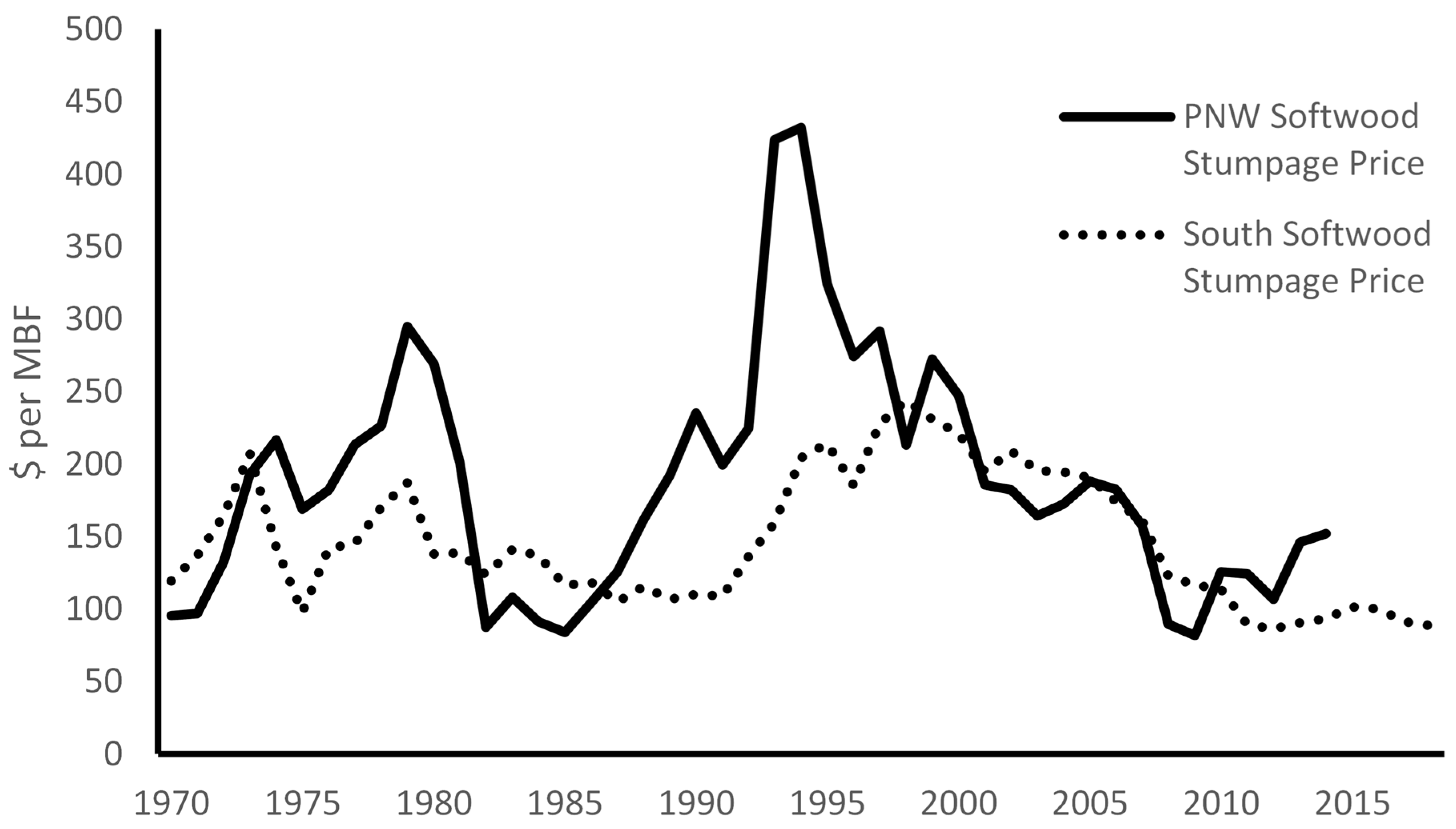
Despite these product-level differences, the econometric evidence strongly supports the existence of an integrated national softwood lumber market. Cointegration analyses using both multivariate Johansen procedures and disaggregate price data across species, regions, and products have found overwhelming evidence for the law of one price in U.S. softwood lumber markets [20,21], indicating that regional prices converge to a single long-run equilibrium. Importantly, Murray and Wear [22] showed that the federal harvest restrictions did not fragment this market but rather strengthened PNW–South price linkages, consistent with active cross-regional arbitrage by buyers when PNW supply contracted. This pattern is also visible in the co-movement of stumpage prices in Figure 2.
The magnitude of the cross-regional investment response is also conditioned by the scale of the supply shock relative to the size of the national market. The federal timber restrictions reduced softwood harvests on public lands in the Pacific Northwest by approximately 49% between the late 1980s and the mid-1990s [13]. At the time, PNW federal forests supplied over 15% of total U.S. softwood timber harvests [17]. The reduction in timber supply from federal forest lands in the early 1990s resulted in a permanent loss of supply from those forests. In the short run, timber harvests can be expanded in other regions and Canada to meet demand [13]. However, wood supply is relatively inelastic in the short run [23,24]. Increasing production by shortening rotation ages can be costly because it reduces future timber value [25]. In addition, some private forests are costly to harvest because they require new infrastructure, such as roads and skid trails. As a result, a portion of the private timber base may not be economically accessible in the near term [26]. In the long run, timber supply can increase through greater investment in timber plantations or improvements in stand productivity [27,28]. However, it takes time for these investments to produce harvestable timber. As a result, changes in forest investment affect regional timber inventories and forest carbon stocks only with a time lag.

3. Methodology

3.1. Theoretical Framework

The long-run supply of timber is determined by the area of intensively managed plantations, the intensity of management on those hectares, the area of natural forests that are available for timber harvesting, and the costs of accessing areas that are inaccessible [7,29]. For the purposes of this study, we start by developing a simple dynamic representation of this complex model. Following the Faustmann tradition in forest economics, we formulate a landowner’s intertemporal optimization problem [30]. The model is derived from adapting the standard forest rotation framework to an aggregate land-use setting in which forest area changes through harvesting and planting and competes with agricultural land. The landowner chooses the harvested area and planted area over time to maximize the present value of profits from timber production, net of planting costs and land opportunity costs.
max π = 0 P t V a t h t C ( t ) g t A ( t ) e r t d t s . t .   X ˙ = h t + g ( t )   h t ,   g t ,   X ( t ) 0   X 0   i s   g i v e n   X t L a n d t A g ( t )
In Equation (1), π is the present value of profit. P(t) is the stumpage price at time t; we assume landowners are price takers and the stumpage price is exogenous. V[a(t)] is the volume per hectare at age a(t), h(t) is the number of hectares harvested at t, C(t) is the per hectare cost of planting, g(t) is the number of hectares planted, X(t) is the total area of forests of all ages, and A(t) is the total rent on forestland. The total area of forest plus agricultural land, Ag(t), should not surpass the size of the total land endowment Land(t). The maximization problem can be solved by forming a Hamiltonian model and solving it. Two useful conditions can be obtained by solving this problem:
P ˙ V a t + P t V ˙ = r P t V a t + A ( t )
C t + t 0 t 0 + t f A ( n ) e r n d n = P t 0 + t f V a t f e r t f
Equation (2) follows the standard Faustmann logic of optimal forest rotation, in which the landowner compares the marginal benefit of delaying harvest with the opportunity cost of holding timber and land for another period [31]. The left-hand side represents the marginal benefit of waiting for a short period before harvest. It consists of the gain from expected stumpage price growth ( P ˙ V a t ) and the gain from incremental timber volume growth ( P t V ˙ ). This treatment is consistent with forest rotation models that allow stumpage prices to evolve over time [32]. The right-hand side represents the marginal cost of waiting. The first term ( r P t V a t ) is the opportunity cost of holding timber capital for an additional period. The second term ( A ( t ) ) is the opportunity cost of keeping land in forest use rather than allocating it to its next best alternative. Landowners choose the rotation age a(t) to set the marginal benefits of waiting to harvest equal to the marginal costs. For stands younger than the optimal rotation age, the marginal benefits of waiting to harvest are driven by expected price growth and volume growth. As a general rule and increase in the price level will lead to lower rotation ages and short-term increases in harvests when the forest area is fixed, as it is for a forest of any age greater than 0 [25].
Equation (3) illustrates that landowners choose the number of hectares to plant, g(t), to set the marginal costs of planting trees, C(t), plus the marginal costs of holding this for a timber rotation, equal to the present value of the marginal benefit, which is the future price times the volume at the age of harvesting. This condition follows the land expectation value logic of forest investment and is consistent with dynamic forest-agricultural land-use models that represent afforestation and reforestation decisions [33]. The rental function is increasing with respect to the total area of land in forests, X(t), such that if the area planted is greater than the area harvested in any year, g(t) > h(t), then the area of plantations increases, and opportunity costs associated with holding plantation forests increase.
The harvest and replanting decisions in Equations (2) and (3) are made separately by landowners. That is, landowners will choose to harvest their trees based on current and near-term growing conditions, price conditions, interest rates, and other factors. Financial return is one of the many objectives of forest management; factors such as trees’ initial stand state, price level, and interest rate can influence landowners’ decision-making over time [26]. We assume there is no constraint on landowners’ finances, meaning they are free to borrow to increase their investments (i.e., the interest rate, r, is exogenous and fixed). They will then choose how much to plant based on their expectations about future prices and growing conditions. Prices are given in the model as a function of exogenous market conditions. When a price shock occurs, landowners have limited options to adjust their behavior in the short run. Harvesting more timber means landowners must harvest successively younger stands, which entails significant opportunity costs and likely results in a lower net return per unit of wood (younger stands typically have a higher proportion of pulpwood-grade biomass and lower prices relative to sawtimber from older, larger trees). For example, the public timber harvesting restrictions of the early 1990s had large price effects not only because timber demand is inelastic, but also because timber is inelastically supplied [25]. That is, it takes large price changes to induce landowners to harvest trees that are still growing rapidly. Over the longer run, however, landowners can increase supply by changing the area of plantations through planting. An increase in the future expected timber price will encourage landowners to rent more land from agriculture and plant trees for timber production (Equation (2)).
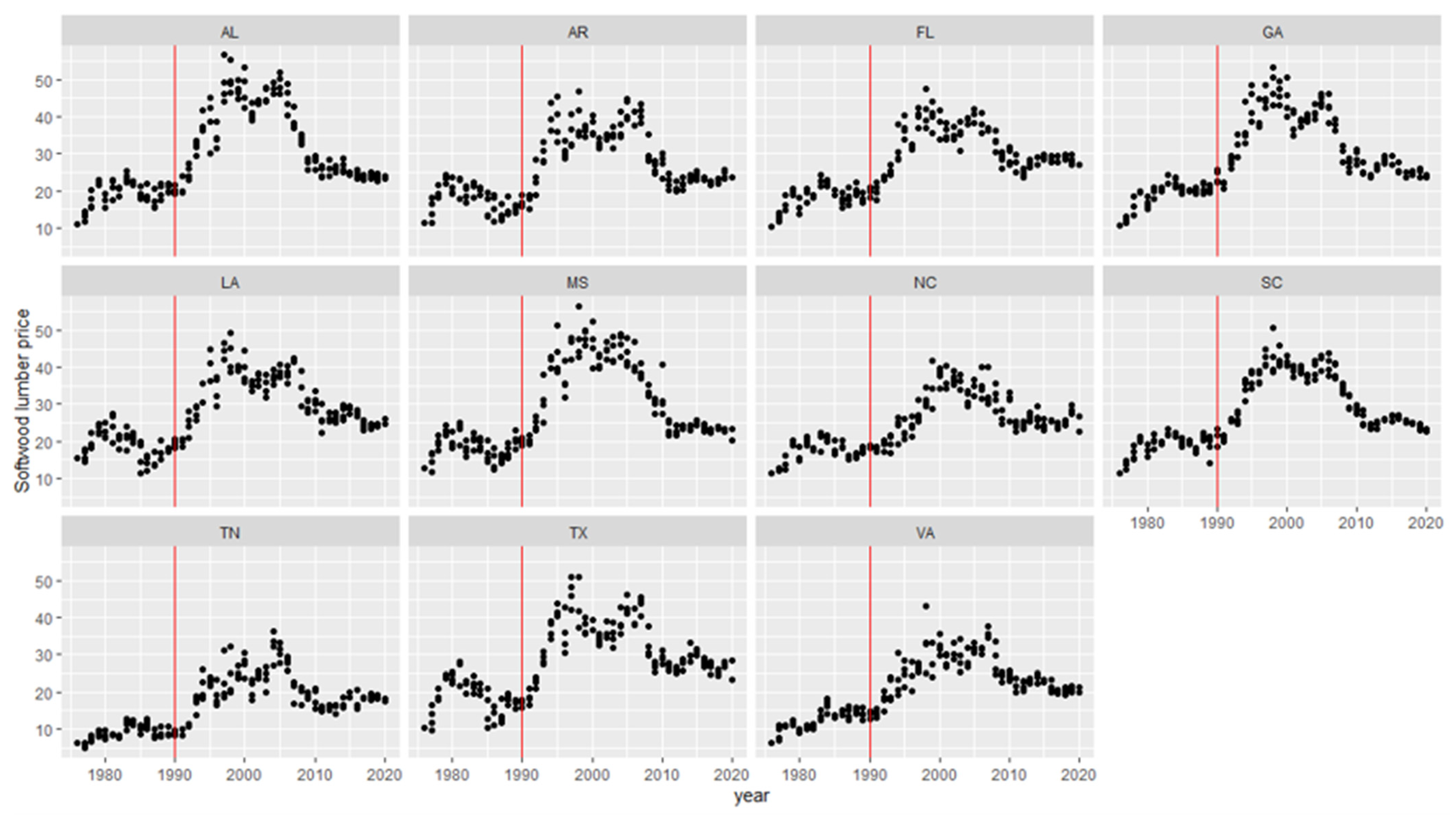
Stumpage prices in the Pacific Northwest U.S. rose throughout the 1980s, while prices in the Southern U.S. remained relatively flat (Figure 2). The price increases in the PNW during this period were driven by strong economic growth and housing demand, especially in the Western U.S., where PNW wood has a competitive advantage relative to other parts of the U.S. and Canada. Although the early 1990s recession likely slowed price growth, prices nonetheless rose from 1991 to 1994, largely due to the shock of timber-harvest restrictions on public land in the Western U.S. Stumpage prices in the Southern U.S. also began rising in 1991. In the South, similar trends emerged in state-level price data (Figure 3), with prices in most states rising sharply after 1990 and peaking around 2000.

3.2. Empirical Specifications

Our empirical strategy has two components. First, we estimate a log-log IV-2SLS specification to obtain consistent price elasticities of planting. Second, we estimate a linear panel fixed-effects model with price–period interactions as a robustness check that does not rely on instrumental variables.
In this analysis, we test whether the policy shift toward lower long-term supplies of timber from federal lands encouraged new softwood planting in the U.S. South. Our theory of change (Figure 1) hypothesizes that harvest restrictions in the Pacific Northwest caused not only a short-term shift in harvesting [13], but also a longer-term structural shift in markets consistent with Equation (2) above. As a result of this structural shift, more hectares were planted in the U.S. South, leading to a longer-run increase in wood volume and wood harvests.
To test whether market conditions in the PNW led to increased forest planting in the U.S. South, we estimate the area of softwoods planted (Yit) in Southern U.S. counties (i) at time (t) as a function of timber prices in the Pacific Northwestern U.S. (PPNWt), timber prices in the Southern U.S. state in which the county is located (PSit), other socioeconomic factors (St), county-level agricultural returns (Ai,t), climatic variables (Cit), and time-stage fixed effects (Zt):
Yi,t = f (PPNWt, PSit, Ait, St, Cit, Zt)
We expect the price impact on planting to be positive, and the policy fixed-effect coefficient in period 3 (1989 to 1996) to be significantly larger than that in period 2 (1982 to 1988). To address the possibility that the southern stumpage price is endogenous, we used a panel fixed-effects instrumental variables (IV) specification. Specifically, we implement a two-stage least squares (2SLS) estimator where the southern stumpage price is instrumented with state-level housing starts, stumpage and pulpwood production in the Southern states, and the major hurricane impact index. The state-level housing starts factor captures the demand-side impact on stumpage prices while stumpage and pulpwood production measures introduce additional supply and demand effects [34]. The major hurricane impact index identifies the states that were affected by level 3 and higher hurricanes between 1978 and 2007, which captures the short-term price shifts due to the major catastrophes [35].
Initially, we aim to estimate the elasticity between price-change impact on planting decisions, so we apply the following equation:
p l a n t i t = A · P s i t β 1 · P p n w t β 2 · e β 3 X + ε i t
where p l a n t i t is the number of acres planted in county i in year t and A = e β 0 . P s i t is the stumpage price in county i in year t. P p n w t is the stumpage price in the PNW region in year t. X are other explanatory indicators. After taking natural logarithms, the equation is rewritten as:
ln p l a n t i t = β 0 + β 1 l n ( P s i t ) + β 2 l n ( P p n w t ) + β 3 X + ε i t
where β 1 and β 2 are the elasticities of prices with respect to planting areas.
Due to the assumption that planting decisions in the current period could be affected by the local price in the previous year, we also test the model with a one-year lagged Southern stumpage price:
ln p l a n t i t = β 0 + β 1 l n ( P s i ,   t 1 ) + β 2 l n ( P p n w t ) + β 3 X + ε i t
where P s i ,   t 1 is the one-year lagged price in county i in year t. It is instrumented by one-year lagged state-level housing starts, stumpage and pulpwood production in the Southern states, and the major hurricane impact index. We also test a model which includes an instrumented southern stumpage price, and add a one-year lagged price as an exogenous variable:
ln p l a n t i t = β 0 + β 1 l n ( P s i t ) + β 2 l n ( P p n w t ) + β 3 X + β 4 l n ( P s i ,   t 1 ) + ε i t
To estimate (4), we also use a two-way (county and year) fixed-effects panel model (1977–2007) with county fixed effect μ i , year fixed effect τ t , policy-period interactions Z t , and county-clustered standard errors; inference is robust to serial correlation and heteroskedasticity within counties. The data for county-level planting in the South covers seven Southern states for the period 1978 to 2007. Our interest in this analysis is whether tree planting increased in the period immediately after the listing of the Northern Spotted Owl as threatened in 1989, relative to other periods in our panel. The categorical variable Zt captures the effect of the policy to restrict timber harvests.
Time fixed effects are included in the model to capture general economic factors influencing markets in the period before 1982, 1982–1988, 1989–1996, and 1997–2007. The pre-1982 fixed effect captures the period before the economic recovery starting in 1983. The 1997–2007 period covers a time of strong housing growth in the U.S. before the financial crisis, as well as the period after the U.S. and Canada reached a softwood trade agreement [36]. The fixed effect model we use is:
Y i t = α 0 + β 1 P i t S + β 2 P i t S × Z t + β 3 P t P N W + β 4 P t P N W × Z t + β 5 C i t + β 6 A i t + β 7 S t + Z t + μ i + τ t + ε i t
The interaction terms between prices and the time-stage dummies allow the marginal effect of price on planting to vary across policy periods, enabling us to test whether price-responsiveness changed after the federal harvest restrictions took effect. Given the time lag between planting and harvesting most trees, stumpage prices are assumed to be exogenous to the planting decision. We include prices from the PNW region, as well as price data for two regions in each state in the South from Timber Mart South. In general, sub-regional prices follow the South-wide trend; however, there are some differences in specific regions due to local supply and demand factors. In general, softwood stumpage prices in the South started rising in the early 1990s and remained high until 2008. The South’s price increases lagged the sharp price rise in the Pacific Northwest that began in the late 1980s.
Exogenous demand and supply factors are captured through the time-dependent dummy variable. To test changes in the relationship between prices and exogenous factors that may affect planting, we include interaction terms between prices and the dummy variables in the model to allow the effect of price on planting to vary over time.
County-level weather and climate are also included in the model. Across the counties in our dataset, average temperature increased by 0.65 °C over the 37-year period, whereas precipitation increased modestly by 4.6 cm over the same period. However, the increase in temperature was concentrated in the northern part of the range, with average temperatures in the northernmost counties increasing by 0.9 °C over the 37-year period, compared to 0.2 °C in the counties further south. Although about 20 cm more precipitation falls annually in the western part of the sample area, neither area displayed a significant trend up or down in annual precipitation over time.

3.3. Data

We construct a panel dataset covering 537 counties across seven Southern U.S. states (AL, FL, GA, MS, NC, SC, and TN). The dataset includes county-level estimates of the annual area of forests planted (specifically, loblolly pine), saw timber prices, agricultural revenues, and climate information (precipitation and temperature). Plot-level observations from the Forest Inventory and Analysis (FIA) dataset are used to estimate total planted area at the county level from 1978 to 2008. FIA is a comprehensive forest inventory database covering the contiguous U.S. with a repeated sampling design. The FIA tracks changes in forest composition, species mix, age class structure, management indicators, and other forest attributes over time. Its standard sampling intensity is approximately one permanent field plot per 6000 acres, implemented through a national hexagonal sampling frame. Within each hexagon, one plot is randomly located. Public FIA coordinates are spatially perturbed and, for some private plots, swapped to protect confidentiality. In this analysis, we are specifically interested in the distinction between planted and natural pine forests.
A consideration in this approach is that the FIA is a probability-based sample survey, not a wall-to-wall census. Its national hexagonal sampling frame allocates approximately one permanent field plot per 6000 acres (~2400 ha), with each plot randomly located within its hexagon to support design-based statistical inference. At this density, the average county in our study area contains several dozen plots. Public FIA coordinates are spatially perturbed and, for some private-land plots, swapped to protect landowner confidentiality, but these privacy protections do not affect the unbiasedness of area estimates at the county level. To further reduce estimation variance, we average multiple independent estimates of each county-year’s planted area derived from successive FIA evaluation cycles.
Climate inputs, including annual average temperature and precipitation rates, are collected from the Prism Climate Group [37] and aggregated to the county level. County-level agricultural prices and production for corn and soybeans are collected from U.S. Department of Agriculture National Agricultural Statistical Service (USDA-NASS) archives to calculate annual gross revenue for each crop, serving as a proxy for cropland rents for the full time series (as county-level cropland rent data are not available for the full time series). The real oil price is sourced from the U.S. Energy Information Administration and used as an indicator of forest management costs. The annual interest rate is collected from the Board of Governors of the Federal Reserve System. Finally, we use a time series of timber price data from TimberMart-South to capture price variation across micro-regions (two per state) in the U.S. South. The agriculture and pastureland area data are collected from USDA-NASS, and the annual housing starts data are from the United States Census Bureau as an indicator of timber demand. Table 1 provides descriptive statistics for the model’s variables.
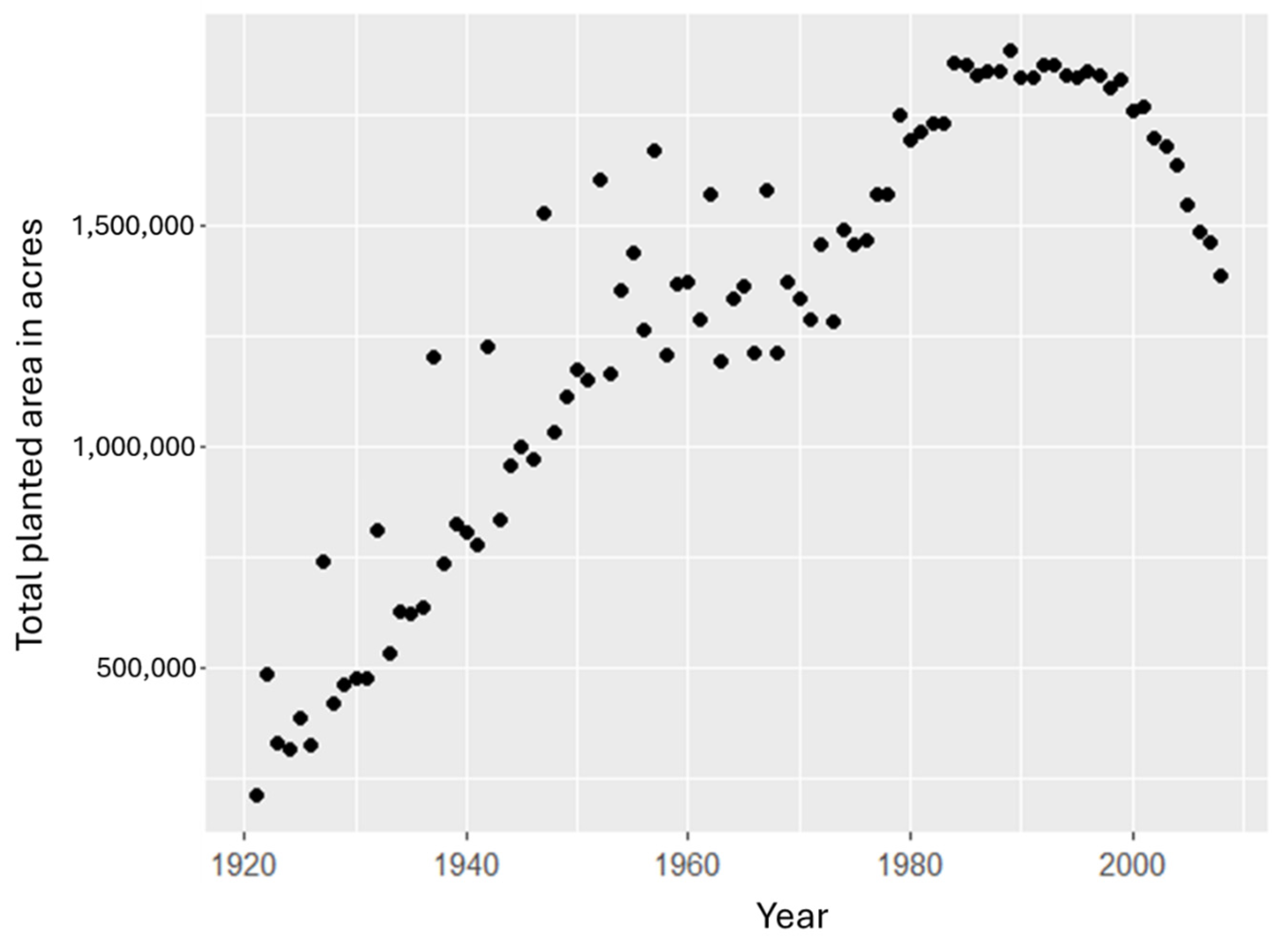
Hernandez, Harper, and South [38] estimate historical tree planting by reviewing and collecting records (before 2000) and sending out survey forms to forest and conservation nurseries (after 2000). Harper et al. [39] provide details on estimating acres planted using surveys. While surveys can provide an overview of planting trends in Southern states, the main limitation of the survey method is that it cannot estimate county-level planting, since conservation nurseries cannot report the number of seedlings they send to each county. Also, the seedlings in conservation nurseries do not reflect the actual planting acreage. Figure 4 presents our estimate of the acres of timberland planted annually in the South using the FIA forest inventory data. The estimation reveals an increasing trend in planting from the 1960s to the 1980s, with peaks in 1959 and 1989.
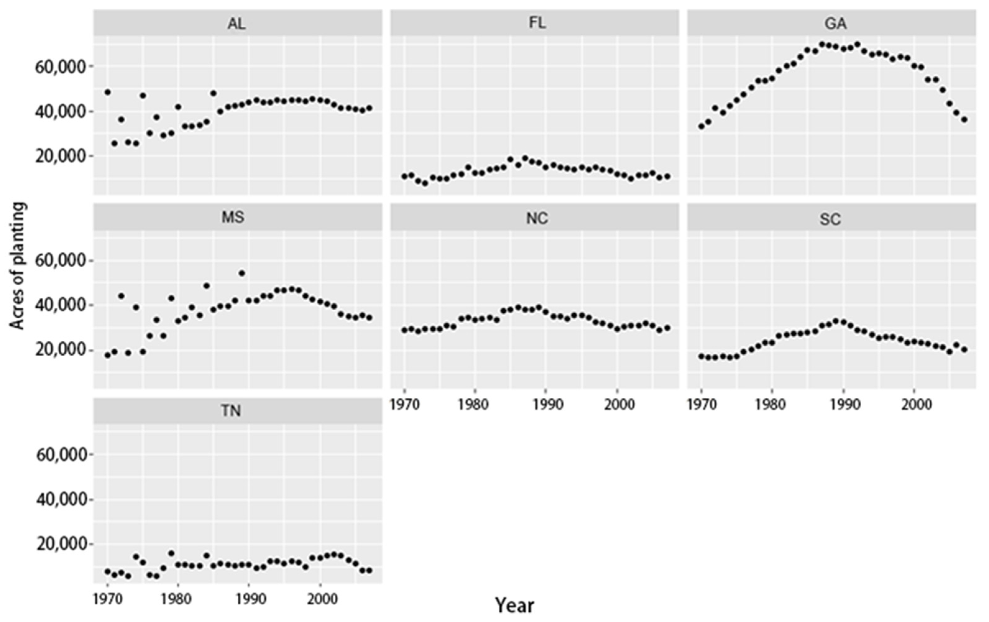
We calculate the area planted in each prior year based on the age-class distribution of the standing forest at the time of the inventory. Since area data were collected in multiple FIA evaluation years, we created multiple estimates of the area planted in each county and year and used the average. For example, if in 2010, a county has 2000 acres of 15-year-old loblolly, then we assume that 2000 acres of loblolly were planted in this county in 1995. And if in 2015, the same county has 2250 acres of 20-year-old loblolly, then we take the average and record that 2125 acres of loblolly were planted in this county in 1995. For counties that do not have planting data in some years, we set planting to 0 in those time periods. Figure 5 shows our estimate of annual loblolly planting area by state from 1970 to 2008. Based on this data, planting peaked in the 1990s in most states.

4. Results

4.1. IV-2SLS Elasticity Estimates

We begin by reporting the IV-2SLS estimates of the log-log specification (Equations (6)–(8)). Three model variants are estimated: Model 1 with the current Southern stumpage price, Model 2 with the one-year lagged price, and Model 3 with both. In all cases, the Southern stumpage price is instrumented as described in Section 3.2. Results are shown in Table 2.
The price coefficients in all three models indicate positive price-elasticities of demand, meaning that when local or regional prices increase, landowners tend to increase planting. The results from models 1 and 2 show that both current and previous prices can affect planting decisions. As model 3 shows, when the current and previous prices are included in the same model, the previous price has a more significant explanatory power for planting decisions.
The time-stage fixed-effect variables capture the direct effects of policies on planting across each period. Our focus is on the fixed effect from 1989 to 1996. The time-stage dummies reveal that a structural break coincides with the 1989 policy rollout. Across all three models, the coefficient on stage 3 (1989–96) exceeds that on stage 2 (1982–88), and Wald tests strongly reject equality (p ≤ 0.001), suggesting that the implemented protection policy is associated with an increase in planting relative to the earlier period, after controlling for prices and climate indicators.
Endogeneity tests reject the null hypothesis of exogeneity, suggesting the importance of IV estimation. However, the Hansen J statistics also reject over-identifying restrictions (p = 0.00), indicating that at least one instrument may violate the exclusion condition or that the model is otherwise not appropriately specified. This may be due to the imperfect data quality since both stumpage and pulpwood production are collected for the entire Southeastern region, and the statistics are the same across every county.

4.2. Linear Panel FE Robustness

We also estimated a linear panel fixed-effects model as a robustness test (Table 3). Due to interactions between prices and time stages, the coefficients on stumpage prices in the Pacific Northwest and the South reflect the price impact on planting in the base period (pre-1982). Higher stumpage prices in this base period in the PNW have a positive effect on planting in the South; however, higher stumpage prices within the state in which the plantation is located have a negative effect on planting in the base period. Price effects in each period are captured by interacting prices with the time dummy variable. These results illustrate that prices have stronger positive effects in the 1980s and 1990s, suggesting strong supply-side effects in which higher prices induce more planting.
Based on economic theory (Equation (2)), annual price changes can also influence harvesting and replanting (i.e., a change in price influences the marginal benefits of holding timber one period to the next), so we include the percentage change in Southern stumpage prices in the models in columns 2 and 3 in Table 3. As expected, this parameter is negative, indicating that a positive annual price change in the previous period is associated with reduced planting, and vice versa. With bigger price increases, the benefits of waiting to harvest trees increase, resulting in trees that are harvested at older ages, for example, when their diameters are large enough to support a higher proportion of sawtimber-grade removals. Holding the forest area constant, this result means fewer hectares will be harvested, and fewer hectares will be replanted. The real logging wage is included in the model in column 3, and the coefficient is significantly negative as expected. Model 3 also includes an estimate of annual softwood production in the Southern States as an additional control on total replanting area after harvest, although this parameter is not statistically significant.
While the baseline price coefficient in the linear fixed-effects model (Table 3) appears negative, this likely reflects the significant endogeneity of stumpage prices and the unique macroeconomic volatility of the late 1970s. As demonstrated in our 2SLS results (Table 2), when demand-side shocks are instrumented, the price impact is positive. Furthermore, the total marginal effect (base price + interaction) remains positive for all post-1982 policy periods.
Although we cannot specifically identify the Northwest Forest Policy relative to the Canadian softwood lumber dispute, the fixed effect coefficients for period 3 (1989–1996) are positive and significant in all three models, and the coefficients for period 4 are also significantly different from 0, suggesting that planting remained strong well after implementation of the Northwest Forest Plan.
Because simple Fixed Effects estimates are known to be biased downward due to price endogeneity in timber markets (as evidenced by the counter-intuitive negative sign in the pre-policy period in Table 3), we rely on the IV-2SLS specification in Table 2 for consistent elasticity estimates. However, the FE model remains useful for illustrating the temporal shift: even with inherent bias, we observe a robust and significant increase in price-responsiveness following the policy implementation.

4.3. Counterfactual Predictions

We predicted the average planted acreage per county for each time stage under four counterfactual scenarios: (i) using observed covariates; (ii) holding the time stage fixed in 1982–1988; (iii) holding prices fixed at their 1982–1988 levels; and (iv) holding both time stage and prices fixed. As reported in Table 4, price variation accounts for a larger share of the change in planting than shifts across periods. Because the specification includes interactions between prices and time stage, the implied price elasticity of planting is larger in Period 2 than in Period 3. Taken together, these predictions indicate that the policy change influenced planting decisions both directly (via the time-stage shift) and indirectly through the price channel. Based on predictions with actual input parameters, we estimate that about 321.5 additional acres of loblolly were planted in each county each year during period 3 (1989–1996), totaling around 173,000 additional acres planted per year in the Southern states, totaling 1.38 million acres during period 3.

4.4. Heterogeneity: Replanting Versus Afforestation

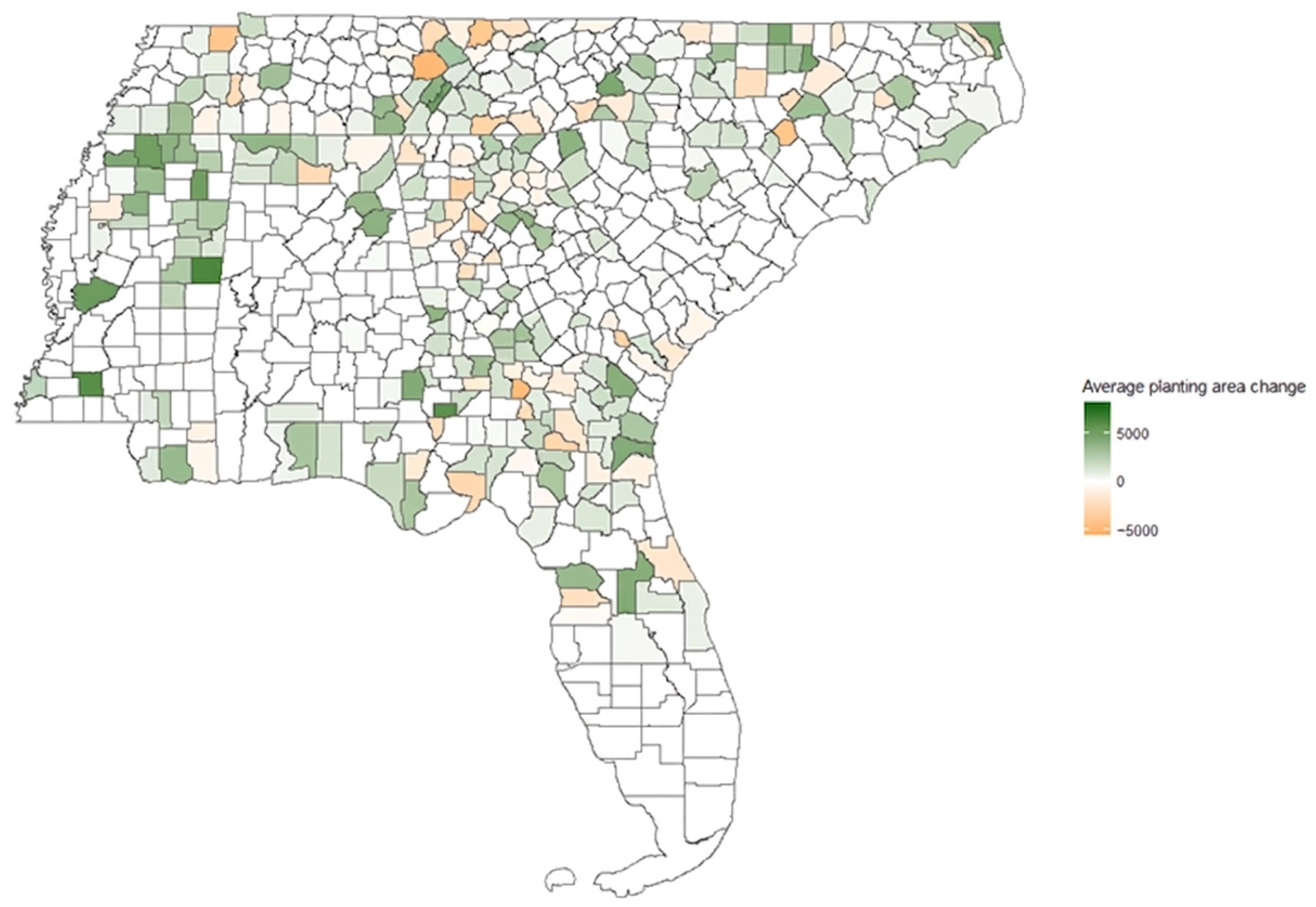
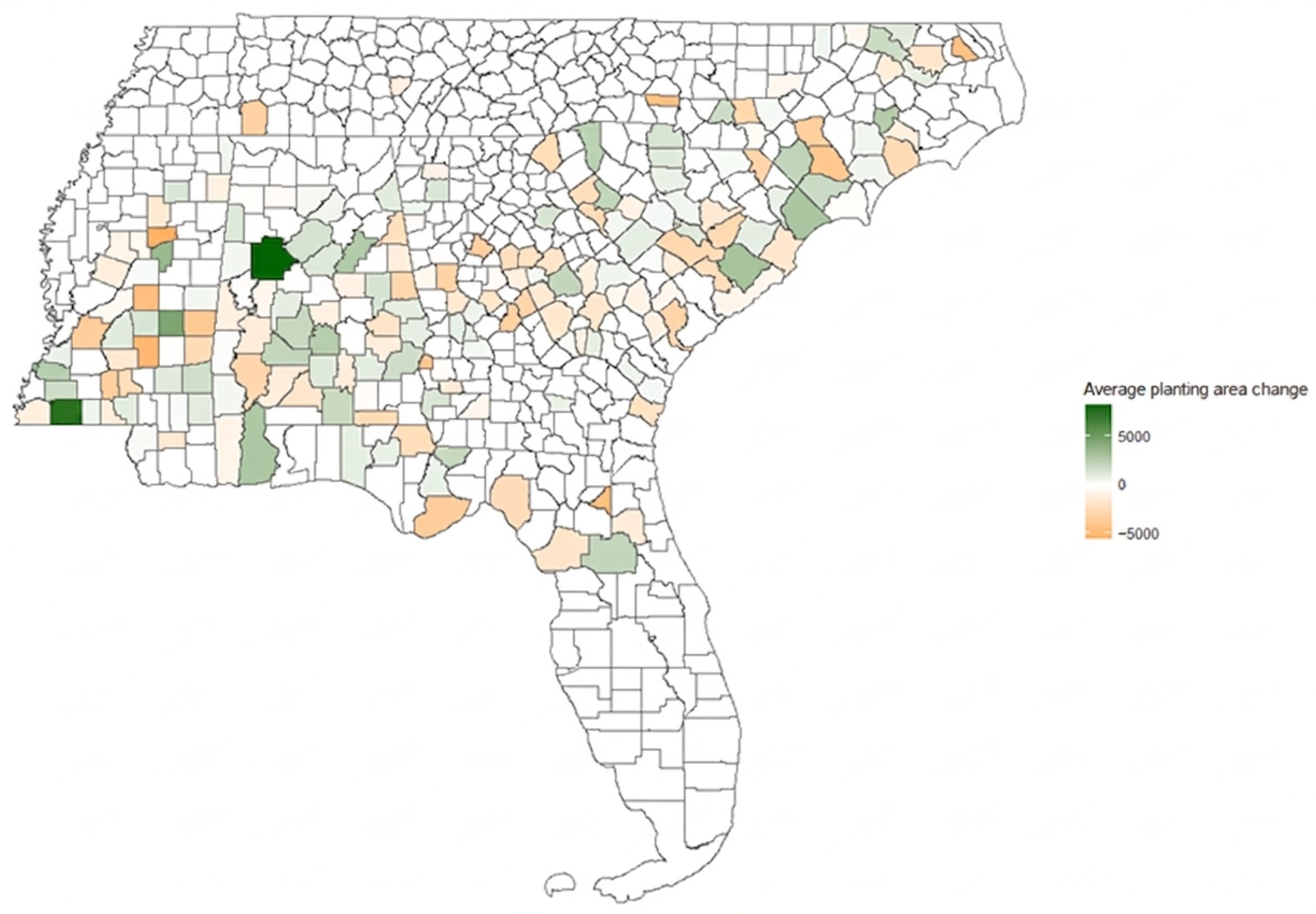
To further assess the importance of replanting versus afforestation in our analysis, we consider differences across counties with relatively larger versus smaller areas of loblolly in the earliest periods. If the time-stage fixed effects are primarily driven by replanting, we expect the effect to be larger in counties with more loblolly hectares, given the observed increase in harvest in the region after the Northwest Forest Plan was implemented [13]. For this analysis, counties are grouped into those with an average of fewer than 5000 acres of loblolly from 1982 to 1988 and those with an average of more than 5000 acres of loblolly from 1982 to 1988. Figure 6 and Figure 7 show changes in the planting area before and after 1989 in each county. It is visually clear that most counties in the group with less than 5000 acres increased loblolly planting after 1989. Among counties in the group with more than 5000 acres, there is no clear pattern indicating whether their planting areas increased after 1989. Table 5 reports the impact of the time-stage on planting areas in each group. The results show that in both the first group (planting area < 5000 acres before policy) and the second group (planting area > 5000 acres before policy), planting area significantly increased after the policy was implemented.

5. Discussion

5.1. Main Findings

This study investigates how the implementation of forest preservation policy in the Pacific Northwest affected softwood planting decisions by private forest landowners in the U.S. South. Using a county-level panel dataset covering 537 counties in seven Southern states over the period 1977–2007, we find evidence that the restrictions were associated with a significant increase in loblolly pine planting in the South, operating through both a direct time-stage shift and an indirect price channel. In our preferred IV-2SLS specification (Table 2), the time-stage fixed effect for the post-policy period (1989–1996) is significantly larger than that for the pre-policy period (1982–1988), and the Wald test strongly rejects equality across periods (p ≤ 0.001). Counterfactual predictions based on the linear fixed-effects model (Table 4) suggest that approximately 321 additional acres of loblolly were planted per county per year during the post-policy period, totaling roughly 173,000 additional acres across these seven Southern states during 1989–1996.
It is well established that softwood harvesting in the Southern U.S. increased after the implementation of the PNW restrictions [13]. Our results reveal that the supply-side response extended beyond short-run harvest reallocation to encompass longer-run investment in new planted forest area. Southern landowners and forest management firms invested more in planting in response to the structural market shift caused by the PNW policy, both replanting recently harvested stands and establishing plantations on previously non-forested land.

5.2. Mechanisms: Replanting vs. Afforestation

An important question for interpreting the carbon implications of our findings is whether the observed increase in planting primarily reflects replanting of recently harvested stands or afforestation of land not previously in forest. Our FIA-derived dependent variable captures total planted area and cannot directly distinguish between the two. However, the heterogeneity analysis in Section 4.4 provides indirect evidence. Counties with fewer than 5000 acres of loblolly in the pre-policy period (1982–1988) showed a clear and broad-based increase in planting after 1989 (Figure 6). By contrast, counties with larger pre-existing loblolly bases (≥5000 acres), where routine replanting after harvest would be expected to dominate planting activity, showed no clear directional pattern (Figure 7). Both groups exhibit statistically significant post-policy planting increases (Table 5), but the pattern is consistent with the small-base counties contributing disproportionately through afforestation, while the large-base counties responded primarily through intensified replanting cycles.
This distinction matters for carbon accounting. Replanting after harvest maintains the existing forest carbon stock but does not add to it on a landscape level, whereas afforestation creates a net addition to the forested land base and, over a rotation cycle, represents a genuine increase in carbon sequestration capacity. The evidence that counties with smaller pre-existing loblolly areas experienced the strongest post-policy planting response suggests that a non-trivial share of the observed planting increase reflects afforestation rather than routine replanting; thus, this represents a genuine offset to the short-run carbon leakage documented in prior studies [11,13].

5.3. Boundary Conditions and Generalizability

Our results demonstrate that forest set-asides in the PNW triggered a measurable long-run planting response in the U.S. South, operating through the price channel of an integrated national softwood market. However, the magnitude of this investment-leakage effect is contingent on several conditions that are particularly favorable in the U.S. context, and readers should exercise caution in extrapolating our specific estimates to other settings.
First, the degree of market integration matters. The U.S. softwood lumber market has been shown to satisfy the law of one price across regions [20,21], and the PNW harvest restrictions appear to have further strengthened cross-regional price linkages [22]. In settings where regional or national wood markets are more segmented, the price transmission that underpins the investment-leakage mechanism would be weaker, and the planting response correspondingly smaller.
Second, the scale and permanence of the supply shock condition the response. The PNW restrictions removed approximately 15% of U.S. softwood supply on a near-permanent basis [13,17], creating a sustained price signal over more than a decade. Temporary or small-scale set-asides would produce weaker and more transient price effects, which may be insufficient to justify the long-term capital commitment involved in establishing new plantations.
Third, the species composition of the set-aside and receiving regions affects the transmission channel. As discussed in Section 2.2, Douglas-fir and loblolly pine are not always perfect substitutes, but they coexist within an integrated national softwood market in which buyers adjust procurement across species in response to relative prices [19,22]. In cases where the conserved and the substitute species serve entirely non-overlapping markets (e.g., tropical hardwoods versus temperate softwoods) the market channel we document here would not operate.
Finally, concurrent policy shocks complicate attribution. The early 1990s coincided with shifts in the U.S.–Canada softwood lumber trade relationship, including the imposition and subsequent expiry of duties and quotas [36]. Although our time-stage fixed effects absorb aggregate demand and trade shocks common across Southern counties, we cannot fully disentangle the Spotted Owl restrictions from the Canada trade dispute in their separate contributions to Southern price increases. This attribution challenge does not undermine our central finding that higher stumpage prices, regardless of their proximate cause, induce long-run planting responses. However, it does limit the extent to which the estimated magnitudes can be ascribed to the Endangered Species Act alone.
In conclusion, these boundary conditions suggest that the investment-leakage mechanism we identify is likely to be a general feature of integrated timber markets subject to large, persistent supply shocks, but that the specific elasticities and magnitudes we estimate are contingent on the institutional, ecological, and market characteristics of the U.S. softwood sector.

5.4. Limitations

As with any empirical study of long-run market responses, our analysis is subject to a couple of data and methodological constraints. First, our county-level planting estimates are derived retrospectively from the age-class distribution of standing forests recorded in periodic FIA inventories, rather than from direct planting records. This introduces measurement noise at the county level; however, because such noise is unlikely to be systematically correlated with the policy treatment, it would bias our estimates toward zero rather than generate spurious positive effects, making our findings conservative.
The Hansen J test for overidentifying restrictions rejects in our IV-2SLS specifications (Table 2), suggesting that at least one instrument may imperfectly satisfy the exclusion restriction. This likely reflects the limited spatial variation in some instruments, particularly the region-level stumpage and pulpwood production data. Importantly, the core qualitative results are consistent across all specifications, including the linear fixed-effects models (Table 3) that do not rely on instrumental variables, which provides reassurance that the central findings are not an artefact of instrument selection.
In addition, our dependent variable captures total planted area without distinguishing replanting from afforestation. While the heterogeneity analysis provides suggestive evidence that afforestation contributed meaningfully to the post-policy response, a precise decomposition is beyond the reach of FIA-based retrospective data and remains an important avenue for future research using direct land-use transition records.
Finally, the early 1990s coincided with shifts in the U.S.–Canada softwood lumber trade relationship [36], and our design cannot fully separate the contribution of the Spotted Owl restrictions from that of the trade dispute. However, this limitation pertains to the attribution of the price shock rather than to our central finding: that sustained stumpage price increases induce long-run planting investment in the South.

5.5. Policy Implications and Future Research

Our empirical estimates contribute to a growing literature on forest carbon leakage and the effects of forest conservation on markets and management decisions. While we do not quantify carbon leakage directly since it would require a systems modelling approach. Our results highlight the need for dynamic accounting frameworks that consider secondary effects (planting responses) and tertiary effects (future harvests from new plantations) in addition to the primary market-induced impact of set-asides (spatial reallocation of harvests). Standard elasticity-based leakage estimation or static views of carbon leakage that consider only carbon gains in set-aside areas and carbon losses in regions experiencing increased harvest may be inadequate when landowners respond to persistent price signals by expanding the planted forest base.
In recent years, the growth of forest carbon markets has introduced an additional revenue stream alongside traditional timber sales, particularly in the U.S. South. Carbon payments can offset planting costs and increase the marginal benefit of delaying harvest, potentially amplifying the investment-leakage mechanism we document here. Future research could extend our framework by incorporating carbon sequestration revenue as an explicit variable and exploring how landowners navigate the trade-off between timber production and carbon market participation under dual price signals.

6. Conclusions

This paper examines the long-run investment response to one of the largest forest set-aside events in U.S. history—the federal timber-harvesting restrictions in the Pacific Northwest following the listing of the Northern Spotted Owl as threatened in 1989. Our principal conclusions are as follows. First, federal timber restrictions in the PNW led to a significant increase in softwood planting in the U.S. South. Using county-level panel data from seven Southern states over the period 1977–2007, we find that planting rates in the post-policy period (1989–1996) were significantly higher than in the preceding period, after controlling for prices, climate, agricultural opportunity costs, and other macroeconomic factors. The effect operates through both a direct structural shift and an indirect price channel, with the latter accounting for a substantial share of the total planting increase. Second, the planting response extends beyond routine replanting to include afforestation. Heterogeneity analysis shows that counties with small pre-existing loblolly bases experienced the strongest post-policy planting increases, suggesting that a meaningful portion of new planting occurred on land not previously in loblolly production. This afforestation component represents a potential net carbon benefit that may partially offset the short-run carbon leakage from harvest reallocation documented in prior studies. Third, standard carbon leakage accounting frameworks need to incorporate long-run investment responses. Static leakage estimates that focus exclusively on the spatial reallocation of harvests following a set-aside will systematically overestimate the net carbon cost of forest conservation policies when those policies induce sustained price signals in integrated timber markets. Our findings underscore the importance of dynamic, intertemporal frameworks that capture both the immediate market adjustment and the subsequent investment response—including changes in planted area, management intensity, and rotation schedules—when evaluating the full carbon implications of forest protection programs.

Author Contributions

Conceptualization, B.L., B.S., and J.S.B.; methodology, B.L. and B.S.; software, B.L.; validation, B.L., B.S., and J.S.B.; formal analysis, B.L.; investigation, B.L. and B.S.; resources, B.S.; data curation, B.L.; writing—original draft preparation, B.L. and B.S.; writing—review and editing, B.L., B.S., and J.S.B.; visualization, B.L.; supervision, B.S.; project administration, B.L. and B.S. All authors have read and agreed to the published version of the manuscript.

Funding

This research received no external funding.

Data Availability Statement

The data presented in this study are available on request from the corresponding author due to the inclusion of proprietary commercial data that cannot be publicly disclosed.

Acknowledgments

This manuscript is part of the Ph.D. thesis of the first author, Bingcai Liu, available online at http://rave.ohiolink.edu/etdc/view?acc_num=osu1669923962916105 (accessed 5 April 2026).

Conflicts of Interest

We certify that the article is the author’s original work. The article has not received prior publication and is not under consideration for publication elsewhere. On behalf of all Co-Authors, the corresponding Author shall bear full responsibility for the submission. This research has not been submitted for publication, nor has it been published in whole or in part elsewhere. We attest to the fact that all Authors listed on the title page have contributed significantly to the work, have read the manuscript, attest to the validity and legitimacy of the data and its interpretation, and agree to its submission to Forests.

References

  1. UNEP; FAO. The State of the World’s Forests: Forests, Biodiversity and People. Available online: http://www.unep.org/resources/state-worlds-forests-forests-biodiversity-and-people (accessed on 25 October 2022).
  2. Griscom, B.W.; Adams, J.; Ellis, P.W.; Houghton, R.A.; Lomax, G.; Miteva, D.A.; Schlesinger, W.H.; Shoch, D.; Siikamäki, J.V.; Smith, P.; et al. Natural Climate Solutions. Proc. Natl. Acad. Sci. USA 2017, 114, 11645–11650. [Google Scholar] [CrossRef] [Scilit]
  3. Austin, K.G.; Baker, J.S.; Sohngen, B.L.; Wade, C.M.; Daigneault, A.; Ohrel, S.B.; Ragnauth, S.; Bean, A. The Economic Costs of Planting, Preserving, and Managing the World’s Forests to Mitigate Climate Change. Nat. Commun. 2020, 11, 5946. [Google Scholar] [CrossRef] [Scilit]
  4. Favero, A.; Daigneault, A.; Sohngen, B. Forests: Carbon Sequestration, Biomass Energy, or Both? Sci. Adv. 2020, 6, eaay6792. [Google Scholar] [CrossRef] [Scilit]
  5. Murray, B.C.; Sohngen, B.; Ross, M.T. Economic Consequences of Consideration of Permanence, Leakage and Additionality for Soil Carbon Sequestration Projects. Clim. Change 2007, 80, 127–143. [Google Scholar] [CrossRef] [Scilit]
  6. Böhringer, C.; Balistreri, E.J.; Rutherford, T.F. The Role of Border Carbon Adjustment in Unilateral Climate Policy: Overview of an Energy Modeling Forum Study (EMF 29). Energy Econ. 2012, 34, S97–S110. [Google Scholar] [CrossRef] [Scilit]
  7. Sohngen, B.; Mendelsohn, R.; Sedjo, R. Forest Management, Conservation, and Global Timber Markets. Am. J. Agric. Econ. 1999, 81, 1–13. [Google Scholar] [CrossRef] [Scilit]
  8. Burtraw, D.; Palmer, K.L.; Bharvirkar, R.; Paul, A. (Eds.) The Effect of Allowance Allocation on the Cost of Carbon Emission Trading; Discussion Paper 01-30; Resources for the Future: Washington, DC, USA, 2001. [Google Scholar]
  9. Kuik, O.; Hofkes, M. Border Adjustment for European Emissions Trading: Competitiveness and Carbon Leakage. Energy Policy 2010, 38, 1741–1748. [Google Scholar] [CrossRef] [Scilit]
  10. Sohngen, B.; Brown, S. Measuring Leakage from Carbon Projects in Open Economies: A Stop Timber Harvesting Project in Bolivia as a Case Study. Can. J. For. Res. 2004, 34, 829–839. [Google Scholar] [CrossRef] [Scilit]
  11. Murray, B.C.; McCarl, B.A.; Lee, H.-C. Estimating Leakage from Forest Carbon Sequestration Programs. Land Econ. 2004, 80, 109–124. [Google Scholar] [CrossRef] [Scilit]
  12. Pan, W.; Kim, M.-K.; Ning, Z.; Yang, H. Carbon Leakage in Energy/Forest Sectors and Climate Policy Implications Using Meta-Analysis. For. Policy Econ. 2020, 115, 102161. [Google Scholar] [CrossRef] [Scilit]
  13. Wear, D.; Murray, B.C. Federal Timber Restrictions, Interregional Spillovers, and the Impact on US Softwood Markets. J. Environ. Econ. Manag. 2004, 47, 307–330. [Google Scholar] [CrossRef] [Scilit]
  14. Oswalt, S.; Miles, P.D.; Pugh, S.A. Forest Resources of the United States, 2017: A Technical Document Supporting the Forest Service 2020 RPA Assessment; U.S. Department of Agriculture, Forest Service, Washington Office: Washington, DC, USA, 2019; 223p. [CrossRef] [Scilit]
  15. Prestemon, J.P.; Wear, D.N.; Abt, K.L.; Abt, R.C. Projecting Housing Starts and Softwood Lumber Consumption in the United States. For. Sci. 2018, 64, 1–14. [Google Scholar] [CrossRef] [Scilit]
  16. Montgomery, C.A.; Gardner, M.B., Jr.; Adams, D.M. The Marginal Cost of Species Preservation: The Northern Spotted Owl. J. Environ. Econ. Manag. 1994, 26, 111–128. [Google Scholar] [CrossRef] [Scilit]
  17. Adams, D.M. Estimated Timber Harvest by U.S. Region and Ownership, 1950–2002; U.S. Department of Agriculture, Forest Service, Pacific Northwest Research Station: Portland, OR, USA, 2006.
  18. Rapp, V. Northwest Forest Plan—The First 10 Years (1994–2003): First-Decade Results of the Northwest Forest Plan; U.S. Department of Agriculture, Forest Service, Pacific Northwest Research Station: Portland, OR, USA, 2008; 42p. [CrossRef] [Scilit]
  19. Nagubadi, R.V.; Zhang, D.; Prestemon, J.P.; Wear, D.N. Softwood Lumber Products in the United States: Substitutes, Complements, or Unrelated? For. Sci. 2004, 50, 416–426. [Google Scholar] [CrossRef] [Scilit]
  20. Yin, R.; Baek, J. Is There a Single National Lumber Market in the United States? For. Sci. 2005, 51, 155–164. [Google Scholar] [CrossRef] [Scilit]
  21. Jung, C.; Doroodian, K. The Law of One Price for U.S. Softwood Lumber: A Multivariate Cointegration Test. For. Sci. 1994, 40, 595–600. [Google Scholar] [CrossRef] [Scilit]
  22. Murray, B.C.; Wear, D.N. Federal Timber Restrictions and Interregional Arbitrage in U.S. Lumber. Land Econ. 1998, 74, 76–91. [Google Scholar] [CrossRef] [Scilit]
  23. Polyakov, M.; Wear, D.N.; Huggett, R.N. Harvest Choice and Timber Supply Models for Forest Forecasting. For. Sci. 2010, 56, 344–355. [Google Scholar] [CrossRef] [Scilit]
  24. Morland, C.; Schier, F.; Janzen, N.; Weimar, H. Supply and Demand Functions for Global Wood Markets: Specification and Plausibility Testing of Econometric Models within the Global Forest Sector. For. Policy Econ. 2018, 92, 92–105. [Google Scholar] [CrossRef] [Scilit]
  25. Sedjo, R.A.; Lyon, K.S. Long-Term Forest Resources Trade, Global Timber Supply, and Intertemporal Comparative Advantage. Am. J. Agric. Econ. 1983, 65, 1010–1016. [Google Scholar] [CrossRef] [Scilit] [PubMed]
  26. Beach, R.H.; Pattanayak, S.K.; Yang, J.-C.; Murray, B.C.; Abt, R.C. Econometric Studies of Non-Industrial Private Forest Management: A Review and Synthesis. For. Policy Econ. 2005, 7, 261–281. [Google Scholar] [CrossRef] [Scilit]
  27. Sedjo, R.A.; Lyon, K.S. The Long-Term Adequacy of World Timber Supply; Routledge: London, UK, 2015. [Google Scholar] [CrossRef] [Scilit]
  28. Henderson, J.D.; Abt, R.C.; Abt, K.L. Forest Carbon under Increasing Product Demand and Land Use Change in the US Southeast. For. Policy Econ. 2024, 167, 103296. [Google Scholar] [CrossRef] [Scilit]
  29. Amacher, G.S.; Ollikainen, M.; Koskela, E. Economics of Forest Resources; The MIT Press: Cambridge, MA, USA, 2009. [Google Scholar]
  30. Faustmann, M. On the Determination of the Value Which Forest Land and Immature Stands Possess for Forestry; Gane, M., Translator; Commonwealth Forestry Institute: Oxford, UK, 1849. [Google Scholar]
  31. Samuelson, P.A. Economics of Forestry in an Evolving Society. In Classic Papers in Natural Resource Economics Revisited; Routledge: London, UK, 2016. [Google Scholar]
  32. Newman, D.H.; Gilbert, C.B.; Hyde, W.F. The Optimal Forest Rotation with Evolving Prices. Land Econ. 1985, 61, 347–353. [Google Scholar] [CrossRef] [Scilit]
  33. Adams, D.M. The Forest and Agricultural Sector Optimization Model (FASOM): Model Structure and Policy Applications; U.S. Department of Agriculture, Forest Service, Pacific Northwest Research Station: Portland, OR, USA, 1996.
  34. Misztal, M.D.; Siry, J.; Mei, B.; Harris, T.; Bowker, J.M. Relation of Pine Chip-n-Saw to Sawtimber and Pulpwood Prices in the Southeastern United States: Direction of Influence. J. For. Bus. Res. 2024, 3, 67–85. [Google Scholar] [CrossRef] [Scilit]
  35. Prestemon, J.P.; Holmes, T.P. Timber Price Dynamics Following a Natural Catastrophe. Am. J. Agric. Econ. 2000, 82, 145–160. [Google Scholar] [CrossRef] [Scilit]
  36. Hoover, K.; Fergusson, I. Softwood Lumber Imports from Canada: Current Issues; Congressional Research Service: Washington, DC, USA, 2015.
  37. Prism Group. Oregon State University. 2019. Available online: https://prism.oregonstate.edu (accessed on 10 December 2019).
  38. Hernandez, G.; Harper, R.; South, D. Historical Periods of Tree Planting in the South. In National Proceedings: Forest and Conservation Nursery Associations—2011; Proc. RMRS-P-68; USDA Forest Service, Rocky Mountain Research Station: Collins, CO, USA, 2012; pp. 7–9. [Google Scholar]
  39. Harper, R.; Hernandez, G.; Arseneault, J.; Bryntesen, M.; Enebak, S.; Overton, R. Forest Nursery Seedling Production in the United States—Fiscal Year 2012; U.S. Department of Agriculture, Forest Service: Portland, OR, USA, 2013; Volume 56, pp. 72–75.
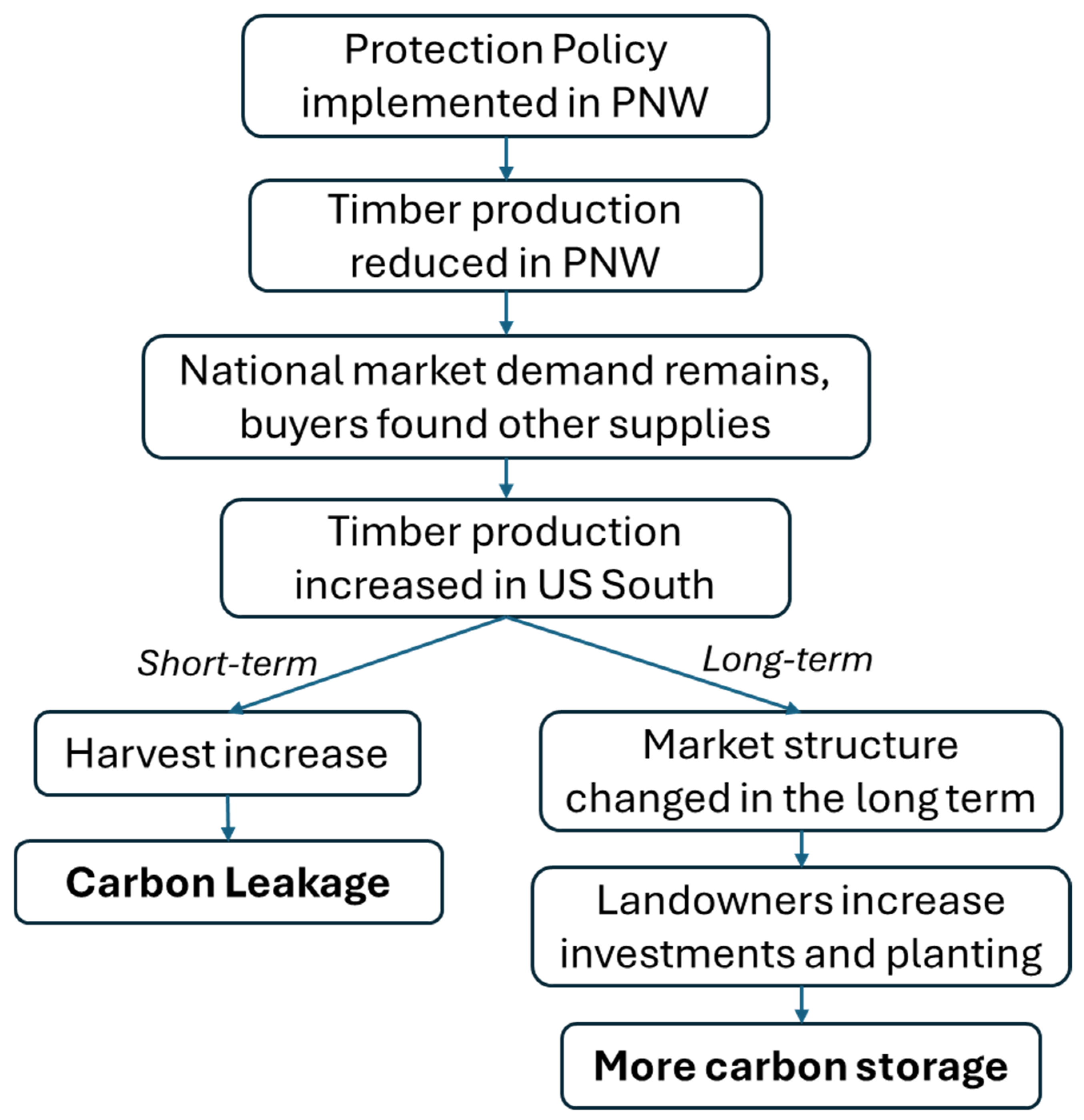
Figure 1. Hypothesized causal pathway guiding analysis on the impact of implementing forest protection policies in the Pacific Northwest (PNW) region.
Forests 17 00604 g001
Figure 2. U.S. softwood prices over time.
Forests 17 00604 g002
Figure 3. Softwood lumber prices in 11 Southern U.S. states. The vertical red line marks the year 1990, which is when the PNW federal forest set-aside occurred. Abbreviations for states are: AL = Alabama; AR = Arkansas; FL = Florida; GA = Georgia; LA = Louisiana; MS = Mississippi; NC = North Carolina; SC = South Carolina; TN = Tennessee; TX = Texas; VA = Virginia.
Forests 17 00604 g003
Figure 4. Acres of timberland planted annually in the South, estimated by FIA forest coverage data.
Forests 17 00604 g004
Figure 5. Annual Loblolly Planting Area in Southern States. Abbreviations for states are: AL = Alabama; FL = Florida; GA = Georgia; LA = Louisiana; NC = North Carolina; SC = South Carolina; TN = Tennessee.
Forests 17 00604 g005
Figure 6. Average loblolly planting area changes by county before and after 1989 (for counties with less than 5000 acres of loblolly between 1982 and 1988).
Forests 17 00604 g006
Figure 7. Average loblolly planting area changes by county before and after 1989 (for counties with more than 5000 acres of loblolly between 1982 and 1988).
Forests 17 00604 g007
Table 1. Summary Statistics for variables used in model (1977 to 2007).
VariableSource
Planting area (Acres, by state)FIA database
Real Stumpage price (PNW, USD per ton, average of whole PNW region)U.S. Forest Service
Real Stumpage price (South, USD per ton, by TimberMart-South regions, there are two regions in each state)TimberMart-South
Annual precipitation (mm)Prism Climate Group
Average temperature (°C)Prism Climate Group
Real oil price (USD)FRED
Nominal Annual interest rate (%)FRED
Annual housing starts (units)United State Census Bureau
Agriculture land area (Acres, by county)USDA NASS
Pastureland area (thousand Acres, by state)USDA NASS
Land area (Acres, by county)USDA NASS
Softwood production in the South (billion board feet)USDA Forest Products Laboratory
Price change compared to the past year (PNW, %)U.S. Forest Service
Price change compared to the past year (South, %)TimberMart South
Ag Return (Corn, USD per acre)USDA NASS
Ag Return (Soybean, USD per acre)USDA NASS
Statistical analyses were conducted using R version 4.1.0 and Stata version 16.
Table 2. County-level panel fixed-effect model with IV estimates by models with different independent variables. The dependent variable is the logarithm of the planting area of county i in year t, from 1978 to 2007.
Model 1
(with Current Southern Price)
Model 2
(with One-Year Lag Southern Price)
Model 3
(with Both Current and One-Year Lag Southern Price)
ln(Southern price)6.28 *** −0.33
ln(one-year lag Southern price) 5.72 ***3.87 ***
ln(PNW price)1.07 **1.19 ***1.37 ***
Annual precipitation0.04 *0.040.03
Average temperature11.70 ***11.91 ***13.43 ***
Precipitation200.000
Temperature2−0.34 ***−0.35 ***−0.39 ***
Real oil price−0.02 ***−0.03 ***−0.03 ***
Annual interest rate0.11 ***0.25 ***0.24 ***
Revenue (Corn)−0.01 ***−0.01 ***−0.01 ***
Revenue (Soybeans)0.00 **0.00 **0.00 **
Period 2 (82–88)2.68 ***2.43 ***2.69 ***
Period 3 (89–96)3.48 ***3.46 ***3.53 ***
Period 4 (97–08)0.350.921.49 ***
Constant−118.66 ***−120.32 ***−129.00 ***
Wald test p value (Period 2 and 3)0.00100.001
Hansen J test p value000
Endogeneity test p value000
Note: * p < 0.1; ** p < 0.05; *** p < 0.01. The Period fixed effect captures the period before the economic recovery starting in 1983. Period 2 and 3 covers the time before and after the conservation policy implemented. The Period 4 covers a time of strong housing growth in the U.S. before the financial crisis, as well as the period after the U.S. and Canada reached a softwood trade agreement. All models include county and year fixed effects. R-squared values reported are within R2 from fixed-effects estimation.
Table 3. County level panel fixed effect estimates by models with different independent variables. Dependent variable is the planting area of county i in year t, from 1978 to 2007.
Model 1
(Base Model)
Model 2
(with Price Change)
Model 3
(with Price Change, Estimated Harvest, and Wage)
Period 2 (82–88) × Stumpage price (PNW)−102.65 ***−97.57 ***−140.20 ***
Period 3 (89–96) × Stumpage price (PNW)−131.31 ***−131.62 ***−157.07 ***
Period 4 (97–08) × Stumpage price (PNW)−128.46 ***−130.82 ***−152.44 ***
Period 2 × Stumpage price (South) 133.83 ***133.78 ***141.48 ***
Period 3 × Stumpage price (South) 114.60 ***115.26 ***118.95 ***
Period 4 × Stumpage price (South) 72.14 **66.64 **71.33 **
Stumpage price (PNW)135.06 ***136.26 ***159.13 ***
Stumpage price (South)−95.56 ***−88.46 ***−93.90 ***
Price Change (South) −325.63 *−307.57 **
Annual precipitation−1.52−0.38−0.40
Average temperature−179.64−143.88−162.14
Precipitation20.010.010.01
Temperature28.287.707.62
Real oil price−13.11 ***−13.85 ***−14.43 ***
Annual interest rate103.07 ***111.40 ***95.26 ***
Annual housing starts−0.005 **−0.005 **−0.004 *
Estimated harvest −68.68
Adjusted logging wage −224.16 ***
Revenue (Corn)−0.75 **−0.78 **−0.81 **
Revenue (Soybeans)0.290.330.21
Period 2 (82–88)4369.57 ***4137.19 ***5558.33 ***
Period 3 (89–96)6088.39 ***6059.54 ***6588.63 ***
Period 4 (97–08)6374.98 ***6603.29 ***7001.64 ***
Constant−1132.30−1826.93901.59
R-squared0.0620.0630.064
Note: * p < 0.1; ** p < 0.05; *** p < 0.01. All models include county and year fixed effects. R-squared values reported are within R2 from fixed-effects estimation.
Table 4. Predictions of average planting area in each period under different scenarios.
Time StageRaw DataPredicted with Actual Input ParametersPredicted with FE Fixed at 82–88Predicted with Prices Fixed at 82–88 LevelPredicted with Prices and FE Fixed at 82–88 Level
Period 1 (before 82)3161.54998.56338.63653.26040.4
Period 2 (82–88)4305.76142.76142.76142.76142.7
Period 3 (89–96)4625.66462.76942.96367.76141.2
Period 4 (Post 96)3838.45674.16818.05645.15651.7
Table 5. County level panel fixed effect estimates by pre-policy planting scale. Dependent variable is the planting area of county i in year t, from 1978 to 2007.
Model Including Counties of Which Planting Area < 5k Acres Before PolicyModel Including Counties of Which Planting Area > 5k Acres Before Policy
Period 2 (82–88) × Stumpage price (PNW)−67.13 **−144.82 **
Period 3 (89–96) × Stumpage price (PNW)−78.45 ***−197.06 **
Period 4 (97–08) × Stumpage price (PNW)−83.76 ***−168.26 **
Period 2 × Stumpage price (South) 101.65 ***58.44
Period 3 × Stumpage price (South) 118.90 ***126.44
Period 4 × Stumpage price (South) 68.21 **185.85 **
Stumpage price (PNW)89.43 ***191.38 ***
Stumpage price (South)−75.22 **−114.90
Price Change (South)26.82−935.41 ***
Annual precipitation7.51−13.49
Average temperature−210.12911.76
Precipitation2−0.030.06
Temperature27.98−20.33
Real oil price−12.74 ***−12.17 ***
Annual interest rate57.49 ***192.54 ***
Annual housing starts−0.01 ***0.00
Revenue (Corn)−0.66−1.38 **
Revenue (Soybeans)0.551.59 *
Period 2 (82–88)2520.35 *8764.95 **
Period 3 (89–96)3057.35 ***9821.16 ***
Period 4 (97–08)4059.66 ***5924.61 *
Constant75.54−12,521.20
R-squared0.0660.097
Note: * p < 0.1; ** p < 0.05; *** p < 0.01. All models include county and year fixed effects. R-squared values reported are within R2 from fixed-effects estimation.
Disclaimer/Publisher’s Note: The statements, opinions and data contained in all publications are solely those of the individual author(s) and contributor(s) and not of MDPI and/or the editor(s). MDPI and/or the editor(s) disclaim responsibility for any injury to people or property resulting from any ideas, methods, instructions or products referred to in the content.