Article

Forestry Tourism Resource Carrying Capacity Prediction Model Based on Multi-Source Data Algorithm

1
College of Economics and Management, Northeast Forestry University, Harbin 150040, China
2
College of History and Tourism Culture, Inner Mongolia Minzu University, Tongliao 028000, China
*
Author to whom correspondence should be addressed.
Forests 2026, 17(5), 534; https://doi.org/10.3390/f17050534
Submission received: 5 March 2026 / Revised: 20 April 2026 / Accepted: 23 April 2026 / Published: 28 April 2026
(This article belongs to the Section Forest Inventory, Modeling and Remote Sensing)

Abstract

To address the challenges of over-reliance on single-source data, strong spatial heterogeneity in scenic areas, and difficulty in dynamically capturing spatial topology and heterogeneous node relationships in forestry tourism resource carrying capacity prediction, this paper constructs a carrying capacity prediction framework that integrates a multi-source data fusion algorithm with an attention mechanism and a GAT-Transformer model. This framework employs a modal-level multi-head cross-attention mechanism to conditionally weight and fuse multi-source heterogeneous data in the node and time dimensions. It adaptively allocates the contribution of each information source based on the spatiotemporal context, suppressing noise and redundant interference. A weighted spatial graph is constructed based on fusion distance, trail connectivity, and traffic similarity. Neighborhood information is aggregated through a graph attention network to characterize spatial heterogeneity. The spatially enhanced node sequence is then input into a multi-layer Transformer encoder to capture the long-term temporal dependence and periodic patterns of carrying capacity. Finally, the prediction results are output through a regression layer. Systematic experiments were conducted using two years of multi-source observation data from Wulingyuan National Forest Park. The results show that the proposed method has low prediction error and good stability, exhibiting excellent performance in temporal scale adaptation, spatial generalization, and resistance to missing data and noise. Simultaneously, the model structure is lightweight, with low inference latency, achieving a good balance between prediction accuracy, interpretability, and engineering deployment.

1. Introduction

With the continuous advancement of ecotourism and rural revitalization policies, forestry tourism has become an important link connecting regional economic development and ecological protection [1,2]. As a core indicator to measure the sustainable reception capacity of scenic spots under the premise of ensuring ecological functions and tourist experience, forestry tourism resource carrying capacity provides an important scientific basis for scenic spot planning, operational management and ecological protection decision-making [3,4]. Traditional carrying capacity assessment methods mainly rely on manual surveys, historical tourist volume statistics or single remote sensing/GIS (Geographic Information System) indicators, which are difficult to reflect the complex spatiotemporal coupling relationships among tourist behavior, facility operation and environmental response [5]. At the same time, forestry scenic areas have significant spatial heterogeneity (such as differences in topography, vegetation, trail structure and facility distribution) and obvious seasonal/holiday fluctuations in tourist flow, which pose severe challenges to the real-time and refined prediction of carrying capacity [6]. To support dynamic management, zoned flow restriction and precise ecological protection of forestry tourism scenic spots, there is an urgent need for a modeling method that can integrate multi-source heterogeneous data, accurately characterize spatiotemporal dependence and provide interpretable prediction results.
Existing research explores the assessment and prediction of forestry and scenic area carrying capacity through multiple pathways, forming a diverse methodological system including statistical analysis, neural network fitting, GIS spatial overlay, fuzzy discrimination, and indicator system construction. These studies have achieved phased results in revealing spatiotemporal patterns, identifying threshold boundaries, and fitting short-term trends [7,8,9]. However, such research generally suffers from problems such as single or coarse data sources, insufficient modeling of spatial topology and heterogeneous node influence mechanisms, limited long-term dependence and emergency scenario response capabilities, and weak model interpretability and uncertainty quantification. These limitations make it difficult to meet the prediction needs of forestry tourism scenarios with strong data heterogeneity and complex spatiotemporal dependencies [10,11,12,13].
In recent years, research in the tourism and forestry fields, addressing the issues of heterogeneous multi-source data and complex spatiotemporal relationships, has gradually shifted towards multi-source data-driven approaches and the fusion of deep spatiotemporal models [14,15,16]. Attention-enhanced sequence models can effectively integrate external variables such as search popularity, weather, and holidays to improve the accuracy of short-term visitor flow prediction; random forests, gradient boosting trees, and other models combine remote sensing images, digital elevation models, and ground observation data to optimize cost and efficiency in forest ecological function assessment; temporal hybrid models and dedicated spatiotemporal Transformers can capture short-term fluctuations and long-term trends simultaneously through self-attention mechanisms; graph neural networks, by explicitly characterizing the spatial relationships of scenic areas, outperform traditional scalar temporal models in multi-step prediction and potential relationship mining [17,18,19]. Multi-source fusion and spatial feature modeling are of great value to the study of forestry tourism carrying capacity, but existing results mostly focus on tourism demand prediction, and there is still a significant gap in research on carrying capacity prediction. Moreover, multi-source fusion is mostly limited to empirical splicing and shallow attention, and lacks sufficient support in terms of modal semantic alignment, missing data processing, interpretability, and uncertainty quantification.
This study uses multi-source data fusion and deep spatiotemporal modeling as its technical approach to construct a high-precision, highly interpretable, and engineering-deployable prediction model for forestry tourism resource carrying capacity. The main research objectives are as follows: (1) to achieve adaptive fusion of multi-source heterogeneous forestry tourism data, enhancing the model’s ability to suppress noise and its robustness to missing data; (2) to accurately characterize the spatial heterogeneity and neighborhood propagation effect of forestry tourism scenic areas, effectively capturing the spatial coupling correlation of carrying capacity between different spatial units; (3) to efficiently capture the long-term temporal dependence and periodic fluctuation characteristics of forestry tourism resource carrying capacity, enhancing the model’s prediction accuracy and generalization ability across multiple time scales; and (4) to ensure a lightweight model structure and low inference latency, achieving a synergistic balance between prediction performance, model interpretability, and engineering feasibility.

2. Multi-Source Feature Fusion and Prediction Model Architecture for Forestry Tourism Resource Carrying Capacity

To present the overall process and inter-module relationships of the forestry tourism resource carrying capacity prediction model in this paper, the overall architecture of the model is shown in Figure 1.
As shown in Figure 1, this architecture takes multi-source heterogeneous data such as remote sensing imagery, tourist trajectory and ticket sales data, geographically labeled social media information, and meteorological and infrastructure operation logs as input. High-level semantic representations of a unified dimension are extracted through feature encoders targeting different modal characteristics. Subsequently, a multi-head cross-attention fusion module is introduced at the feature level to adaptively weight the contributions of different data sources under different spatiotemporal contexts, mitigating the problems of modal heterogeneity and information redundancy.

2.1. Spatiotemporal Feature Engineering and Modality Transformation

All raw data are first unified into a common spatiotemporal network to ensure consistency in subsequent end-to-end modeling. Let G = { g i } i = 1 N represent the set of spatial units (grids or nodes) obtained by dividing the study area, where N is the number of units. The time axis is divided into hours, denoted as T = { t 1 , , t T } . All modal data are mapped to spatiotemporal unit pairs (gi, t).
(1)
Spatial Aggregation of Trajectory and Point Data
Before spatial aggregation of trajectory and point data, this paper first unifies the coordinates and projections, reprojecting all vector/point data and images to a unified projection coordinate system, specifically using UTM (Universal Transverse Mercator), and aligning the raster reference to ensure that the spatial mapping function π ( p ) g i for any point p is uniquely determined, where π ( p ) represents the mapping from point to cell.
Let P i , t be the set of original location points mapped to cell gi within the time window t . The aggregation feature of trajectory/location data on g i , t is calculated as follows: x i , t traj = Agg { β ( p ) : p P i , t } , where β ( p ) is the measure of a single point; the function Agg is the mean; and x i , t traj represents the trajectory feature vector. β ( p ) includes dwell time, movement speed, and visit count index, and then x i , t traj = [ dur ¯ i , t ,   sv ¯ i , t , count i , t ] , where dur ¯ i , t is the average dwell time; sv ¯ i , t represents the average movement speed; and count i , t = | P i , t | represents the number of location points falling into this cell within the time window, used to characterize the intensity of visitor flow.
(2)
Remote Sensing/Image Feature Extraction and Spatial Downsampling
For the available multispectral images at each time point, the pixel-level ecological index NDVI (Normalized Difference Vegetation Index) is first calculated, as defined in Equation (1) [20,21].
NDVI ( x , y ) = R NIR ( x , y ) R R ( x , y ) R NIR ( x , y ) + R R ( x , y )
R NIR ( x , y ) represents the near-infrared reflectance at spatial location (x,y), reflecting the reflection characteristics of vegetation to near-infrared electromagnetic radiation; R R ( x , y ) represents the red reflectance at spatial location (x,y), reflecting the reflection characteristics of vegetation to red electromagnetic radiation.
The image features of grid cell g i are obtained by pixel-weighted averaging, as shown in Equation (2).
x i , t img = 1 | PI i , t | pi PI i , t ϕ pixel ( v )
In the equation, PI i , t is the set of pixels falling into cell gi at time t; ϕ pixel is a predefined pixel feature (NDVI); and x i , t img represents the remote sensing/image feature vector.
(3)
Text Modal Representation and Time Series Features
For each text o (with timestamp and geographic tag), the Chinese pre-trained language RoBERTa (Robustly Optimized Bidirectional Encoder Representations from Transformers Pretraining Approach) model is applied to obtain the sentence vector δ ( o ) [22]. Unit-level sentiment/topic features are represented by a weighted average, as shown in Equation (3).
x i , t text = 1 | O i , t | o O i , t δ ( o )
x i , t text represents the text feature vector; O i , t is the set of texts mapped to gi,t; and if empty, the mask m i , t text = 0 is set.
To capture daily/weekly/seasonal characteristics, lag features and sliding statistics are constructed for each unit, as shown in Equation (4).
l i , t ( k ) = x i , t k ,   μ i , t ( wid ) = 1 wid s = 1 wid x i , t s , σ i , t ( wid ) = 1 wid s = 1 wid ( x i , t s μ i , t ( wid ) ) 2
k is the lag order, and wid is the sliding window width. For periodic encoding, Fourier basis functions are used to encode the time points. l i , t ( k ) represents the lag feature; μ i , t ( wid ) and σ i , t ( wid ) represent the mean and variance of the sliding window, respectively. x i , t s represents the feature value of the i-th entity at time point t − s, where s is an integer from 1 to wid .
The meteorological modal feature x i , t met is obtained from meteorological stations within the study area and aligned with time t according to spatial unit g i . This paper selects fundamental meteorological variables that significantly affect tourist travel and scenic area carrying capacity to form the feature vector: x i , t met = [ Temp i , t , Hum i , t , Prec i , t , Wind i , t ] : Temp i , t represents temperature (°C); Hum i , t represents relative humidity (%); Prec i , t represents precipitation (mm); and Wind i , t represents wind speed (m/s). If a time unit is missing, it is imputed using spatial proximity interpolation and temporal Kalman smoothing, and the missing mask is recorded simultaneously for subsequent attention fusion.

2.2. Feature-Level Multi-Head Attention Fusion Module

To avoid scale inconsistencies and noise accumulation caused by simple splicing, this paper uses a modality-specific encoder and multi-head cross-attention for feature-level alignment and weighted fusion. Let there be C modalities. The original features of modality c at unit gi and time t are denoted as x i , t ( c ) .
(1)
Linear Mapping and Location-Time Information Injection
This paper constructs a modality encoder for each modality to map the original features to a unified dimension. Image features are represented by ResNet50 (Residual Network 50 layers), which is then reduced to a unified dimension via a fully connected layer [23]. Trajectory/flow features are extracted using 1D-CNN (1D Convolutional Neural Network) and reduced to a unified dimension. Text sentiment features are reduced to a unified dimension using RoBERTa pooling vectors via FC (Fully Connected) [24,25]. Meteorology/facilities features are reduced to a unified dimension using MLP (Multilayer Perceptron). If the corresponding mask m i , t ( c ) = 0 , the encoding is skipped and replaced with a zero vector, while the mask information is retained to be passed to the attention layer.
After mapping the original features, positional and temporal encodings are added to each encoded vector, as shown in Equation (5).
z ~ i , t ( c ) = z i , t ( c ) + W p p i + W time time t
W p and   W time are the linear projection matrices corresponding to the positional and temporal encodings, respectively. p i and time t are the positional and temporal encodings, respectively. z ~ i , t ( c ) represents the vector after positional and temporal encoding.
(2)
Multi-Head Cross-Attention Calculation
A linear transformation parameter is constructed for each head h. The single-head attention output is shown in Equation (6) [26,27].
head h ( u i , t , { z ~ i , t ( c ) } ) = c M α i , t , h ( c ) V i , t , h ( c ) Q i , t , h = W h Q u i , t , K i , t , h ( c ) = W h K z ~ i , t ( c ) , V i , t , h ( c ) = W h V z ~ i , t ( c )
u i , t represents the learnable query basis vector; W h Q , W h K , and W h V are the linear transformation parameters; α i , t , h ( c ) represents the attention weights; and V i , t , h ( c ) represents the value vector.
Attention weights are defined by a masked softmax dot product, as shown in Equation (7) [28].
α i , t , h ( c ) = exp Q i , t , h , K i , t , h ( c ) / d h + b i , t ( c ) c M exp Q i , t , h , K i , t , h ( c ) / d h + b i , t ( c )
, represents the vector dot product; the constant d h is the scaling term; the bias term b i , t ( c ) is set to −∞ (through masking) when the modality is missing so that the corresponding weight is zero; when the modality exists, b i , t ( c ) = 0; and M represents the context set.
(3)
Output Mapping and Gated Fusion
Finally, all head outputs are concatenated and linearly mapped to obtain the fused representation, as shown in Equation (8).
MultiHead ( u i , t , { z ~ i , t ( c ) } ) = W O h e a d 1 ; ; h e a d H
W O is the output projection matrix, and the semicolon indicates vector concatenation.
To balance the main representation and modal information, a gating mechanism is introduced, and residual connections and layer normalization are performed, as shown in Equation (9).
g i , t = sigmoid ( W g [ u i , t ; MultiHead ( ) ] + b g ) , h i , t = LayerNorm ( u i , t + g i , t MultiHead ( ) )
⊙ represents element-wise multiplication; g i , t represents the gating mechanism; and h i , t is the final fused vector, which serves as the input for the subsequent spatial GAT. W g represents the weight matrix of the gating mechanism, and b g represents the bias term of the gating mechanism.

2.3. Spatial Graph Construction and GAT Node Update

2.3.1. Spatial Graph Construction

Before constructing the forestry tourism resource carrying capacity prediction model, this paper first constructs a spatial graph, then updates the node representation using GAT at each time step, and finally performs Transformer encoding on the time series of each node to capture long-range temporal dependencies.
This paper is based on the spatial unit set G = { g i } i = 1 N of the study area constructed above, where the primary fusion feature of the i-th unit at time t is h i , t . First, a weighted undirected graph is constructed according to deterministic rules. The edge weights are constructed using three types of complementary quantization standards and linearly synthesized, as follows:
The three types of complementary quantization are the spatial distance attenuation component w ij ( dist ) , the trail connectivity component w ij ( conn ) , and the historical flow correlation component w ij ( flow ) , defined as shown in Equation (10).
w ij ( dist ) = exp ( - γ di di ij ) w ij ( conn ) = Co ij κ ij w ij ( flow ) = rel ij + 1 2
di ij represents the Euclidean distance between gi and gj (under a unified projection), and γ di is the distance attenuation coefficient, set according to the spatial scale of the study area. Specifically, it is the reciprocal of the average distance between the center points of all adjacent spatial units, so that the distance weight has a reasonable attenuation range within the study area scale. Co ij indicates that g i and g j are directly connected in the trail or road network. Its value is determined by the topology map constructed from the trail vector data in GIS. If there is a trail that directly connects spatial units g i and g j , then Co ij = 1 ; otherwise, it is 0. κ ij represents the optional weight scalar given by the connected edge according to the trail’s accessibility. rel ij represents the Pearson correlation coefficient between nodes calculated based on the node flow sequence (observed passenger flow) during the training period.
The final combined weights are weighted and standardized, as shown in Equation (11).
w ~ ij = ω 1 w ij ( dist ) + ω 2 w ij ( conn ) + ω 3 w ij ( flow )
ω 1 to ω 3 represent the weights determined by the validation set, which are then row-normalized to obtain the adjacency matrix.
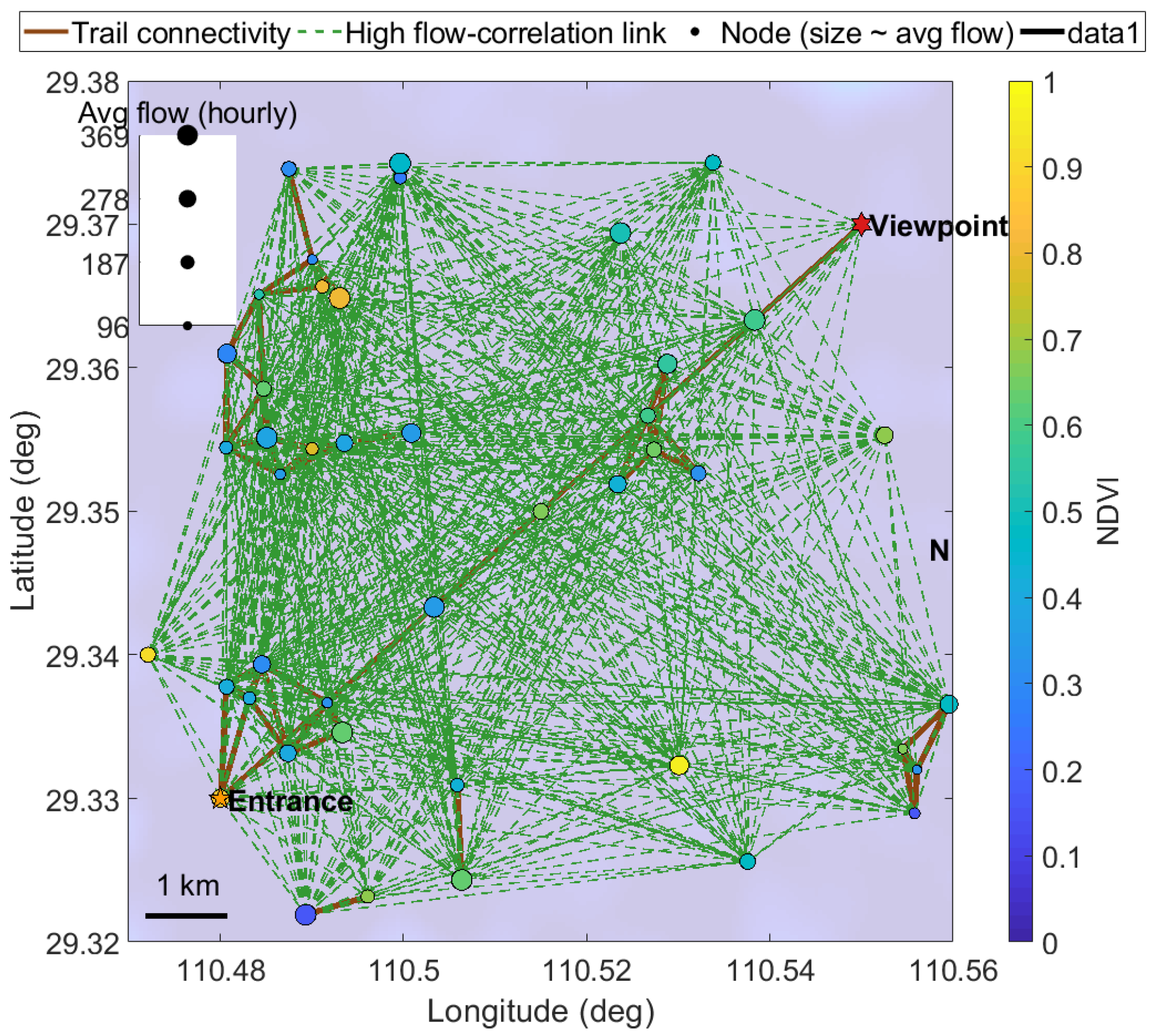
In predicting the carrying capacity of forestry tourism resources, constructing a reasonable spatial graph structure is the foundation for subsequent graph attention networks to characterize spatial relationships. Its role is to depict the comprehensive connections between different scenic spot units in terms of geographical proximity, connectivity of tour routes, and similarity of tourist flow behavior, thus providing structured input for comparing the predictive performance differences between “independent node modeling” and “spatial relationship modeling.” The spatial graph construction is shown in Figure 2.
Figure 2 shows the spatial graph construction result of the study area, where the horizontal axis represents the longitude of each node, and the vertical axis represents the latitude. The circular nodes represent the divided scenic spot spatial units, and the node color represents the vegetation cover status. Solid lines represent strong connections constructed based on spatial distance and trail connectivity, and dashed lines represent weak connections constructed based on the temporal correlation of tourist flow. The nodes in the study area exhibit a strip-like and cluster-like structure distributed along the main tourist routes, and entrances and core viewing nodes show high connection density, reflecting their pivotal role in tourist flow organization.

2.3.2. GAT Node Update

At each time step t , GAT is applied to the node features to perform spatial information aggregation. Let the learnable linear transformation of the l-th layer be W ( l ) , and let the attention parameter vector be a ( l ) . Then, for each directed neighbor ( i , j ) , the unnormalized attention coefficient is calculated as shown in Equation (12) [29].
e ij , t ( l ) = LeakyReLU ( a ( l ) T [ W ( l ) h i , t W ( l ) h j , t ] )
The symbol indicates vector concatenation, and LeakyReLU (Leaky Rectified Linear Unit) is an activation function with a small slope. h i , t represents the feature vector of node i at time step t, containing the node’s current state information. h j , t represents the feature vector of node j at time step t, i.e., the feature of node i’s neighbor node j.
Based on Equation (12), using adjacency masking, numerical stabilization, and scaling, the normalized attention weights are obtained, as shown in Equation (13).
α ij , t ( l ) = exp ( e ij , t ( l ) ) 1 { A ij > 0 } j N i exp ( e ij , t ( l ) ) 1 { A ij > 0 }
α ij , t ( l ) represents the normalized attention weights; e ij , t ( l ) represents the unnormalized attention coefficients; A ij represents the adjacency mask matrix. N i represents the set of neighbors of node i.
This paper employs multi-head attention to enhance representational power. The number of heads is denoted as H. Each head is independently parameterized and outputs a vector. Finally, at the end of the layer, the layer output is obtained by concatenation or averaging, and residuals and layer normalization are applied, as shown in Equation (14).
h ^ i , t ( l ) = LayerNorm h i , t ( l 1 ) + Concat h = 1 H j N i α ij , t ( l , h ) W ( l , h ) h j , t ( l 1 )
In the equation, h i , t ( 0 ) = h i , t . W ( l , h ) is the projection matrix of the h-th head in the l -th layer, and LayerNorm represents layer normalization. To improve robustness, attention discarding and output discarding are applied at the attention weights and node representations, respectively.
Finally, L layers of GAT are stacked to expand the spatial receptive field, and at each time step, the spatially enhanced node representation h ~ i , t = h ^ i , t ( L ) is output. This representation numerically adapts the influence intensity of different neighbors on the target node through learnable attention coefficients, thereby characterizing heterogeneous node relationships and topological propagation paths in the scenic area, and solving spatial coupling problems such as trail connectivity and the propagation of local congestion to the neighborhood.

2.4. Node-Based Temporal Transformer Encoder

After spatial encoding in GAT, its output is fed into a temporal Transformer encoder for long-range temporal dependency capture. For each node gi, its spatially augmented representation sequence { h ~ i , t T + 1 , , h ~ i , t } over T time steps is collected, and this sequence is used as the input to the Transformer encoder to model long-range temporal dependencies and the impact of holidays/sudden events. Let the input matrix be Hi, with the s-th row being h ~ i , t T + s .
First, positional encoding is injected into the temporal dimension. A learnable temporal positional embedding is used to obtain the positional input, as shown in Equation (15).
X i ( 0 ) = H i + Pos
Pos represents the learnable temporal positional embedding, and X i ( 0 ) represents the positional input. If there are events or exogenous markers (such as holidays or rainfall events), the corresponding event vector is added to the corresponding time step to form a correction to X i ( 0 ) .
Each encoding layer of the Transformer consists of a multi-head self-attention network and a feedforward network. For the l-th layer, the linear mapping matrices W Q ( l ) , W K ( l ) , and W V ( l ) are defined. The unnormalized similarity for time positions s and r in the l-th layer is shown in Equation (16) [30,31].
ζ s , r , i ( l ) = W Q ( l ) X i , s ( l 1 ) , W K ( l ) X i , r ( l 1 ) d h
In the equation, ζ s , r , i ( l ) represents the unnormalized similarity; d h represents the dimension per head, and d h = d / H .
Normalization is then performed under an optional future information mask to obtain the attention weights, as shown in Equation (17).
π s , r , i ( l ) = exp ( ζ s , r , i ( l ) ) 1 { M s , r causal = 1 } r = 1 T exp ( ζ s , r , i ( l ) ) 1 { M s , r causal = 1 }
In the equation, M s , r causal represents the future information mask, and π s , r , i ( l ) represents the attention weight. Here, M s , r causal masks the future position when causal constraints are required (such as teacher-mandated or autoregressive training); otherwise, it is fully open to obtain the full historical and recent global context. The head-level output is calculated based on the attention weight and then merged to obtain the hierarchical attention output, as shown in Equation (18) [32].
Attn ( l ) ( X i ( l 1 ) ) s = Concat h = 1 H r = 1 T π s , r , i ( l , h ) W V ( l , h ) X i , r ( l 1 )
Attn ( l ) ( X i ( l 1 ) ) s represents the hierarchical attention output.
Then, the layer output is formed by passing it through a feed-forward neural network (FFN) (two fully connected layers with activation functions), residuals, and layer normalization, as shown in Equation (19).
X i ( l ) = LayerNorm ( X i ( l 1 ) + Dropout ( Attn ( l ) ( X i ( l 1 ) ) ) ) X i ( l ) = LayerNorm ( X i ( l ) + Dropout ( F F N ( X i ( l ) ) ) )
X i ( l ) represents the layer output.
After stacking the LT layers, the output vector of the last time step is taken as the temporal context representation, as shown in Equation (20).
s i , t = X i ( l T ) [ T , : ]
[ T , : ] represents the last row of the sequence (the encoded representation of the latest time step), which is then used as the input of the regression head for carrying capacity prediction.
To reduce the computational burden of the Transformer on long sequences, local window attention and stratified temporal sampling are employed in this study, which limit the range of r values during attention normalization while retaining the core structure of the model.

3. Forestry Tourism Resource Carrying Capacity Prediction Performance Evaluation System

3.1. Experimental Data

The study area selects Wulingyuan National Forest Park in Zhangjiajie City, Hunan Province as the research object. Data collection covers the period from 1 January 2022 to 31 December 2023 (two years). Remote sensing and aerial photographic data include publicly available Sentinel-2 multispectral imagery (approximately 150 images, L2A level) for seasonal vegetation and land cover analysis, and orthophotos (resolution approximately 5–10 cm) generated from 12 aerial photographs of the park’s core scenic area conducted by UAVs (unmanned aerial vehicles) during the study period for micro-feature extraction of trails and scenic spots. Basic geographic elements are provided by the Zhangjiajie Forestry Bureau, including vector layers of park boundaries, trail network, viewpoints, and service facilities. All raster/vector data undergo unified projection and rasterization for subsequent registration.
Visitor behavior and traffic data consist of multi-source operational records, including hourly visitor entry counts from ticket sales and entrance counters, totaling approximately 17,520 hourly records and anonymized mobile location data provided by telecommunications operators with data-sharing agreements with the scenic area, aggregated into 45,000 trajectory records and approximately 1,100,000 location points, used to generate rasterized heatmaps and OD (Origin-Destination) flow matrices; in addition, 12,000 geotagged social media posts and reviews (including timestamps and sentiment text) are captured and preprocessed for visitor perception and preference analysis. Meteorological and environmental monitoring data comes from hourly records (temperature, rainfall, wind speed, approximately 17,520 records) from the nearest weather station and scenic area facility operation logs (hourly records of parking space occupancy, toilet maintenance, etc.). All data involving personal location or text are anonymized and aggregated before collection, and only spatial unit/temporal window level aggregation features are used in the analysis to protect privacy.

3.2. Validation Scheme and Baseline Comparison

This paper constructs a unified data partitioning and experimental evaluation scheme, and selects several representative models as control baselines. All models are used on the same dataset with a consistent 70% training set, 15% validation set, and 15% test set partitioning, and unified input features, prediction step size, and training epoch settings to ensure the comparability of experimental results and avoid configuration bias. The control models cover different modeling paradigms, including ARIMA (Auto regressive Integrated Moving Average), XGBoost (eXtreme Gradient Boosting), ATT-BiLSTM and Transformer; STGCN (Spatial-Temporal Graph Convolutional Network) and GCN-LSTM (Graph Convolutional Network-Long Short-Term Memory); and BiLSTM + Transformer. Experimental parameters are shown in Table 1.

4. Carrying Capacity Prediction Performance

4.1. Comparison of Global Prediction Accuracy and Prediction–Actual Comparison Curves

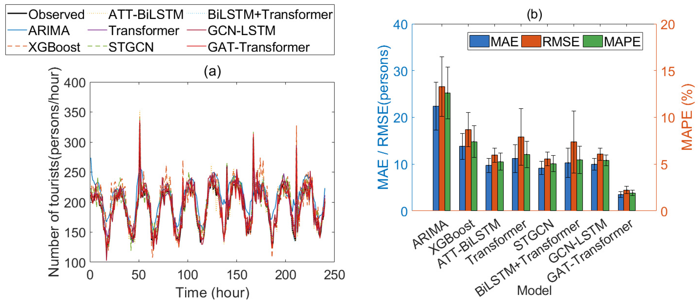
To systematically compare the overall performance differences of different prediction models in the task of predicting the carrying capacity of forestry tourism resources, this paper conducts a global prediction accuracy comparison and prediction–actual comparison analysis on the test set. The core function of this analysis is to quantify the fitting ability and stability of each model to changes in tourist scale through a unified error index, thereby determining which prediction is more accurate and stable, and to intuitively examine the model’s ability to characterize periodic fluctuations and sudden disturbances through time series comparison.
The experiment selects mean absolute error, root mean squared error, and mean absolute percentage error as evaluation indicators, reflecting the magnitude of prediction deviation, sensitivity to large errors, and relative error level, respectively, to comprehensively measure model performance from a complementary perspective. The global prediction accuracy comparison and prediction–actual comparison curves are shown in Figure 3.
As can be seen from Figure 3a, traditional statistical models and some machine learning models exhibit significant lag or over-smoothing during peak and sudden fluctuation phases. In contrast, the GAT-Transformer model in this paper fits the actual curve well under periodic variations, weekend effects, and random sudden disturbances, exhibiting the smallest overall bias. The quantitative results in Figure 3b further validate this conclusion. The GAT-Transformer model has an MAE of 3.54 ± 0.62 individuals, an RMSE of 4.45 ± 0.78 individuals, and an MAPE (Mean Absolute Percentage Error) of only 1.93 ± 0.28%, significantly lower than all the compared models.

4.2. Time Scale Performance

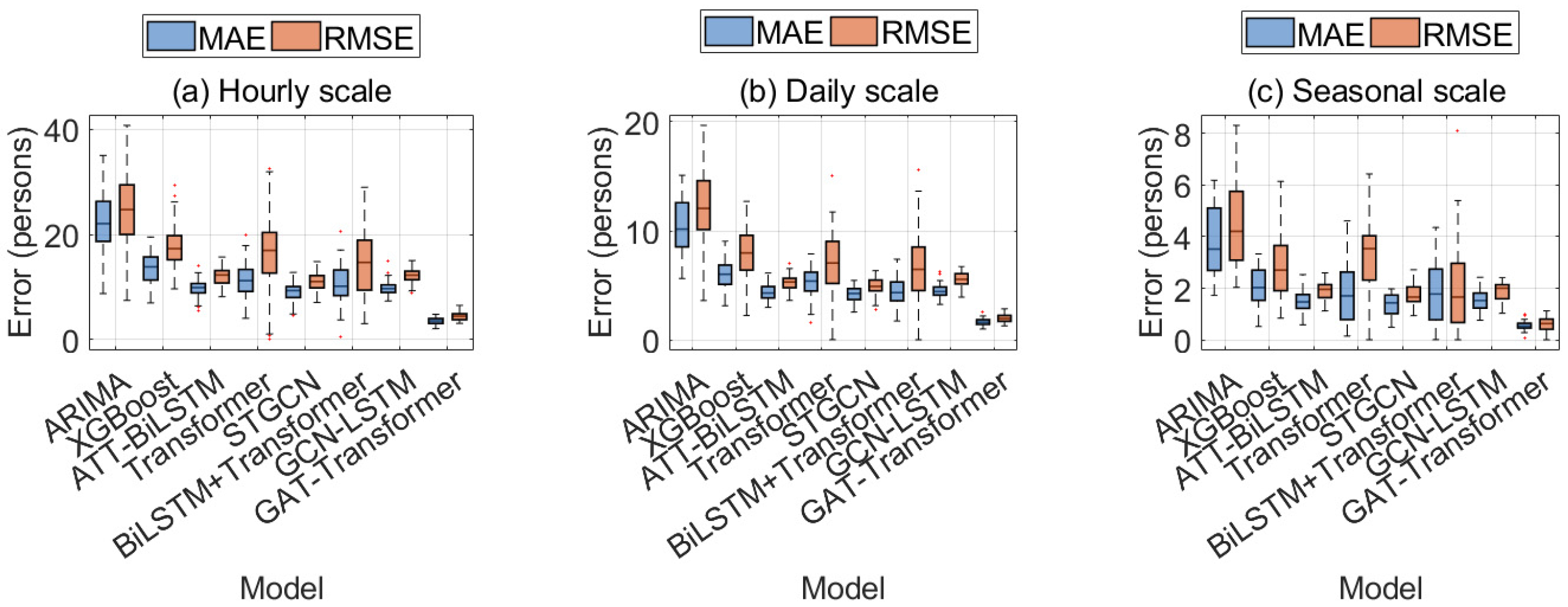
The time scale performance is shown in Figure 4. The horizontal axis of Figure 4 represents different prediction models, and the vertical axis represents the error value.
As shown in Figure 4a–c, the GAT-Transformer model performs best across all time scales. The hourly MAE is 3.56 ± 0.61, and the RMSE is 4.41 ± 0.73; the daily MAE decreases to 1.64 ± 0.30, and the RMSE is 1.95 ± 0.37; the seasonal MAE further decreases to 0.55 ± 0.19, and the RMSE is 0.64 ± 0.27, demonstrating its advantage in capturing complex spatiotemporal dependencies. In contrast, the traditional ARIMA model has a larger error, with an hourly MAE as high as 22.18 ± 5.27 and an RMSE of 25.10 ± 6.46. Although the seasonal MAE decreases somewhat, it is still significantly higher than the GAT-Transformer model, indicating poor sensitivity to short-term fluctuations. The XGBoost, ATT-BiLSTM, and STGCN models perform moderately. STGCN, in particular, achieves an hourly MAE of 9.16 ± 1.65 and an RMSE of 10.93 ± 1.67, indicating that spatiotemporal graph convolution can partially capture the spatial correlations between nodes. However, it still slightly underperforms the GAT-Transformer model under high-frequency fluctuations.

4.3. Spatial Generalization Ability

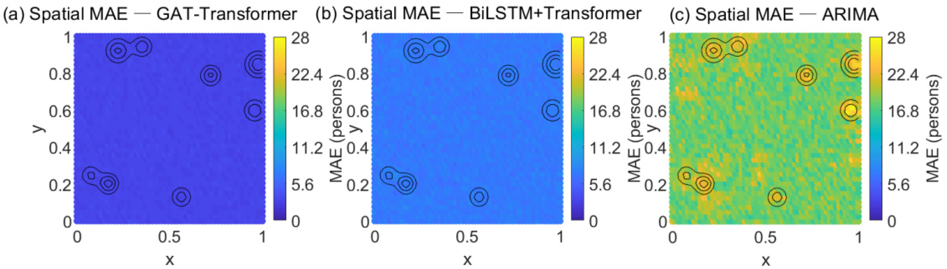
To evaluate the model’s generalization ability in unseen spatial regions, this paper uses spatial mean absolute error (MAE) as the evaluation index. By statistically analyzing the mean absolute error of each grid (or node) over the entire prediction period, the spatial deviation between the predicted results and the actual values is measured. The spatial generalization analysis results are shown in Figure 5.
As can be seen from Figure 5, GAT-Transformer (Figure 5a) has the smallest overall Spatial MAE, with a uniform error distribution and relatively low errors in areas with high facility density or undulating terrain, indicating that this model can effectively capture spatial dependencies and local features. BiLSTM + Transformer (Figure 5b) has a slightly higher overall error, with larger errors in some areas with high facility density or complex terrain, indicating that this model is not as sensitive to spatial heterogeneity as GAT-Transformer. ARIMA (Figure 5c) has the largest errors in hotspot areas and grids with obvious terrain undulations, showing its lack of ability to model spatial structures.

4.4. Modal Contribution Ablation

The modal contribution ablation analysis is shown in Table 2. The columns ΔMAE, ΔRMSE, and ΔMAPE represent the percentage change relative to the full modal baseline, with positive values indicating performance degradation, i.e., increased error.
As shown in Table 2, removing the trajectory modality has the greatest impact on model performance. MAE increases from 3.54 to 5.10 (+44.1%), RMSE from 4.45 to 6.20 (+39.3%), and MAPE from 1.93% to 2.78% (+44.0%), indicating that trajectory information is crucial for capturing real-time visitor flow and dynamic visit volume. Removing the remote sensing modality leads to an increase in MAE to 4.30 (+21.5%), RMSE to 5.30 (+19.1%), and MAPE to 2.35% (+21.8%), demonstrating that the spatial terrain and coverage information provided by remote sensing significantly enhance the model’s spatial generalization ability. Removing the social media modality results in an MAE of 3.95 people (+11.6%), an RMSE of 5.05 people (+13.5%), and an MAPE of 2.20% (+14.0%). Removing the meteorological modality results in an MAE of 3.85 people (+8.8%), an RMSE of 4.78 people (+7.4%), and an MAPE of 2.05% (+6.2%). This indicates that these two modalities provide auxiliary information, helping to capture sudden events and short-term environmental disturbances, respectively.

4.5. Interpretability Test of Attention Weights

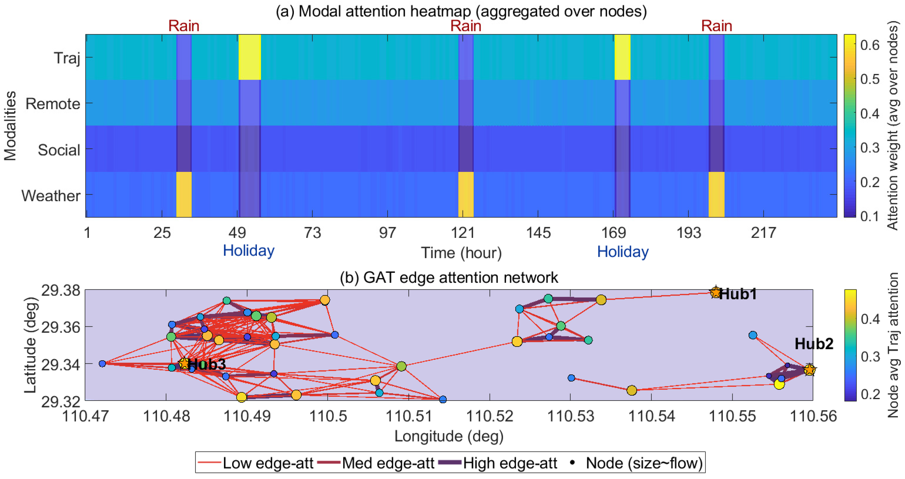
To deeply analyze the role of multi-source data in carrying capacity prediction, this paper conducts an interpretability test on attention weights, focusing on evaluating the relative contributions of different modalities at each time point and the impact of spatial correlations between nodes on the prediction results. The interpretability test of attention weights is shown in Figure 6. In Figure 6a, the horizontal axis represents time, and the vertical axis represents various modalities; the color intensity indicates the average attention weight magnitude. In Figure 6b, the node positions correspond to geographical coordinates; the node size reflects the average flow rate; the color represents the attention weight of the trajectory mode; the thickness and color of the edges characterize the strength of spatial correlations between nodes.
As can be seen from Figure 6a, the attention of the trajectory modality increases significantly during holiday windows (hours 50–56 and 170–174), with the average weight increasing by about 0.3 compared to non-holiday periods, reflecting that tourist behavior significantly enhances the importance of trajectory data during holidays. During rainfall windows (hours 30–34, 120–124, and 200–204), the attention weight of the meteorological modality increases significantly, with an average increase of about 0.4, indicating that weather events have a direct impact on the prediction model. Figure 6b shows that high-traffic nodes typically have higher trajectory attention and form dense edge connections with neighboring nodes. Edges with weights above 0.06 are mainly concentrated in hub areas, indicating that the model spatially assigns higher attention weights to key traffic and activity nodes.

4.6. Robustness Testing Against Missing Data and Noise

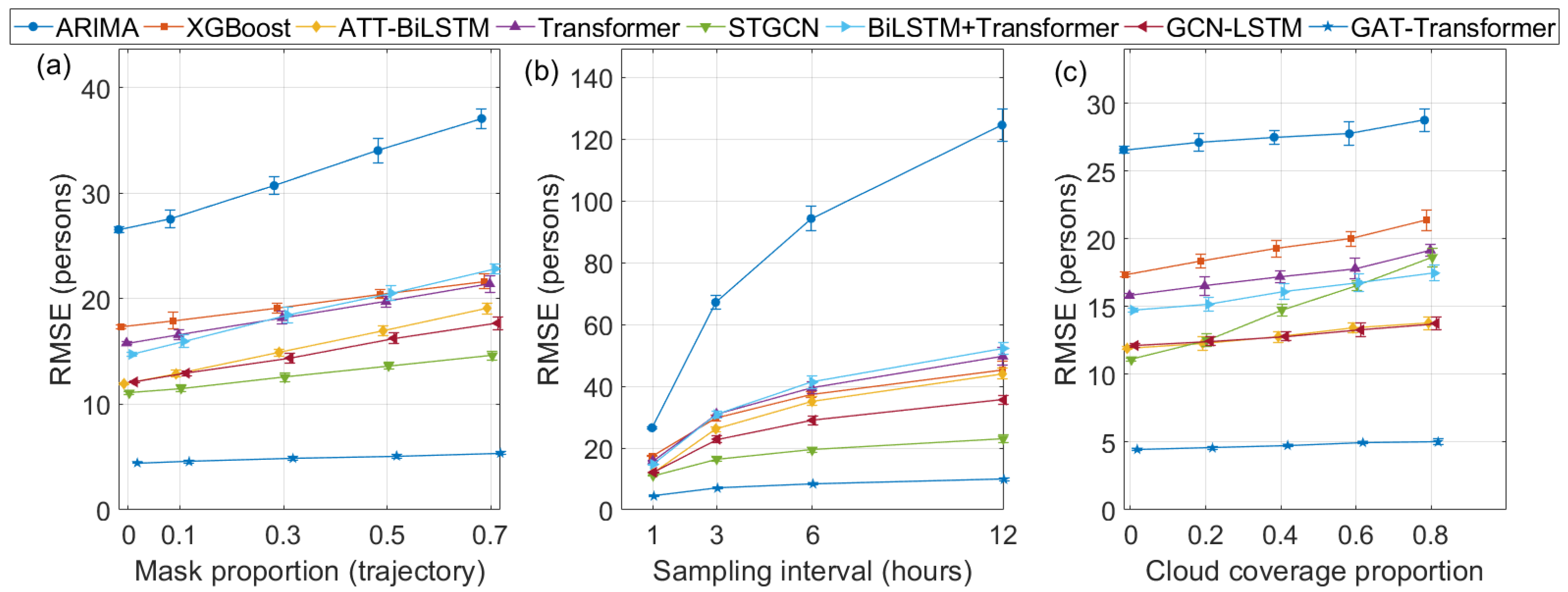
To systematically evaluate the stability and reliability of the model in real-world applications when faced with incomplete data and observational noise, this paper conducts robustness testing against missing data and noise. In actual forestry tourism carrying capacity prediction, multi-source data often becomes missing or degraded due to equipment failure, changes in sampling strategies, or remote sensing cloud obstruction. The robustness testing against missing data and noise is shown in Figure 7. Figure 7a–c shows the results for the three scenarios, with the horizontal axis representing the perturbation intensity and the vertical axis representing RMSE.
As shown in Figure 7a, as the random mask ratio of the trajectory mode increases from 0 to 0.7, the RMSE of each model shows a monotonically increasing trend, but the growth rate differs significantly. The RMSE of ARIMA increases from 26.56 to 37.08, ATT-BiLSTM from 11.93 to 19.09, while the GAT-Transformer model only increases from 4.45 to 5.37, and its standard deviation remains at a low level of 0.04–0.19, indicating that this model has the strongest robustness to missing trajectory data. This difference mainly stems from the fact that the GAT-Transformer model uses a graph attention mechanism to compensate for information in the spatial neighborhood, effectively utilizing relevant node features when some node data is missing. Figure 7b shows that temporal downsampling has the most significant impact on the model. When the sampling interval increases from 1 h to 12 h, the RMSE of ARIMA rises sharply to 124.51, while that of the GAT-Transformer model only rises to 9.85. The increases in STGCN and GCN-LSTM are also smaller than those of pure time series or weak time series models. This indicates that models that explicitly model spatiotemporal dependencies can mitigate the performance degradation caused by the sparsity of temporal information. In Figure 7c, the increase in cloud coverage mainly affects models that rely on remote sensing features. The RMSE of STGCN increases from 11.08 to 18.62, a significantly higher increase than that of the GAT-Transformer model (4.45 → 5.01) and GCN-LSTM (12.12 → 13.75).

4.7. Computational Efficiency and Deployability Indicators

The computational efficiency and deployability metrics are shown in Table 3. Size FP32 (32-bit Floating Point) represents the actual storage overhead of the model at 32-bit floating-point precision; and CPU (Central Processing Unit) and GPU inference latency respectively characterize the online response performance of the model under general computing power and accelerated computing power conditions.
Table 3 shows that ARIMA and XGBoost, due to their simple structure and extremely small parameter count (≤0.05 M), have significant advantages in training time (≤0.5 GPU·h) and inference latency (CPU ≤ 6 ms), but their performance improvement is limited by the model’s expressive power. Among deep learning models, ATT-BiLSTM, STGCN, and GCN-LSTM achieve a good balance between parameter size (1.8–2.8 M) and inference latency (GPU 2.5–3.0 ms), indicating that the computational cost does not increase linearly after introducing temporal or spatial modeling. In contrast, BiLSTM + Transformer and the standard Transformer, due to their multi-layered attention and recurrent structures, show a significant increase in parameter count and training time (up to 4.0 M, 10 GPU·h), and a significant increase in CPU inference latency. The GAT-Transformer model presented in this paper slightly outperforms some baselines in terms of parameter count (3.6 M) and training time (12 GPU·h), but its GPU inference latency is still controlled at 3.5 ms, which is better than hybrid models with similar structures.

5. Conclusions

5.1. Theoretical Implications

This study constructs a forestry tourism resource carrying capacity prediction framework based on multi-source data and GAT-Transformer, which has important theoretical implications for the research of forestry tourism and spatiotemporal prediction. First, the study breaks through the limitation of single-source data in traditional carrying capacity prediction, and designs a node-time conditional multi-modal cross-attention mechanism to realize the adaptive fusion of multi-source heterogeneous data (trajectory, remote sensing, social media, meteorology, etc.). This mechanism not only solves the problems of modal heterogeneity and information redundancy in multi-source data fusion, but also improves the model’s ability to suppress noise and deal with missing data, providing a new method for multi-source data fusion in the field of tourism resource assessment. Second, the study constructs a weighted spatial graph based on distance, trail connectivity and historical traffic similarity, and uses GAT to explicitly model the spatial heterogeneity and neighborhood propagation effects of forestry tourism scenic areas. This design makes up for the deficiency of traditional time series models that ignore spatial structure, and enriches the theoretical research of spatial modeling in tourism carrying capacity prediction. Third, the study combines GAT with Transformer to construct an end-to-end spatiotemporal joint modeling structure, which can simultaneously capture the spatial dependencies and long-term temporal dependencies of forestry tourism resource carrying capacity. This structure provides a new theoretical framework for the spatiotemporal prediction of complex geographic phenomena, and can be extended to other fields such as urban traffic flow prediction and ecological environment monitoring.

5.2. Practical Implications

The research results of this paper have important practical implications for the operational management and ecological protection of forestry tourism scenic areas. First, the GAT-Transformer model constructed in this paper achieves high-precision prediction of forestry tourism resource carrying capacity (MAE = 3.54 ± 0.62), and can maintain good prediction performance across different time scales and spatial regions. Scenic area managers can use the prediction results of the model to carry out dynamic management and zoned flow restriction of tourist flow, which can not only ensure the tourist experience, but also prevent the damage of excessive tourist flow to the forest ecological environment, realizing the sustainable development of forestry tourism. Second, the model has strong robustness to missing data and noise, and can maintain stable prediction performance under the conditions of trajectory data missing, temporal data sparsity and remote sensing cloud cover. This makes the model suitable for the complex actual application scenarios of forestry tourism scenic areas, and has high practical value. Third, the model maintains a lightweight structure and low inference latency, which can realize the real-time prediction of carrying capacity. Scenic area managers can deploy the model on the intelligent management platform of the scenic area to obtain the real-time carrying capacity prediction results of each spatial unit, and carry out precise and real-time management of the scenic area. In addition, the interpretability test of the model’s attention weights shows that the model can adaptively adjust the contribution of different data modalities according to the spatiotemporal context, and the spatial attention weights have clear physical meaning. Scenic area managers can use the attention weight results of the model to identify the key influencing factors of carrying capacity and the core spatial units of the scenic area, providing a scientific basis for the optimization of the scenic area’s layout and the improvement of service facilities.

5.3. Limitations of the Study

Although this study has achieved certain research results, there are still some limitations that need to be improved in the follow-up research. First, the current model still relies on the prior construction of the spatial graph of the scenic area, and the weight parameters of the spatial graph (ω1, ω2, ω3) are determined by the validation set, which lacks the dynamic adaptive adjustment ability of the spatial graph structure with the change in tourist flow and scenic area environment. Second, the model’s ability to characterize extreme sudden events is limited. These extreme events will lead to drastic changes in tourist flow and carrying capacity of the scenic area, and the current model is trained based on historical data, which is difficult to capture the characteristics of such extreme events. Third, the study only verifies the model with the multi-source data of Wulingyuan National Forest Park, and the generalization ability of the model to other types of forestry tourism scenic areas needs to be further verified. Fourth, the model does not consider the interaction between tourist behavior and carrying capacity, and only takes tourist trajectory data as the input feature, without modeling the decision-making process and behavioral preferences of tourists.

5.4. Future Research Directions

Based on the limitations of this study, the future research directions are as follows: First, introduce the dynamic spatial graph construction method, design a graph structure learning module that can adaptively adjust the spatial graph topology and edge weights according to the real-time data of the scenic area, and improve the model’s ability to capture the dynamic spatial relationships of the scenic area. Second, integrate the extreme event detection and modeling module into the model, collect the data of extreme events in forestry tourism scenic areas, construct an extreme event feature set, and use the few-shot learning or transfer learning method to improve the model’s ability to characterize extreme sudden events. Third, expand the research sample, collect the multi-source data of different types of forestry tourism scenic areas, and verify the generalization ability of the model across different scenic areas. At the same time, carry out cross-scenic area model fine-tuning to improve the adaptability of the model to different types of scenic areas. Fourth, combine the tourist behavior decision model with the carrying capacity prediction model, introduce the tourist behavior theory and discrete choice model, model the tourist’s travel decision-making process and behavioral preferences, and improve the interpretability and prediction accuracy of the model. Fifth, introduce online incremental learning and causal constraint modeling into the model, realize the real-time update of the model with the new data of the scenic area, and explore the causal relationship between multi-source factors and forestry tourism resource carrying capacity, so as to provide more in-depth scientific support for the management of forestry tourism scenic areas.

Author Contributions

Writing—original draft, Y.M.; Writing—review & editing, Y.G. All authors have read and agreed to the published version of the manuscript.

Funding

This research received no external funding.

Institutional Review Board Statement

Not applicable.

Informed Consent Statement

Not applicable.

Data Availability Statement

The data that supports the findings of this study are available within the article.

Conflicts of Interest

The authors declare no conflicts of interest.

References

  1. Peng, J.; Li, J.; Peng, L.; Zhang, Y. Forest Ecosystem Conservation Through Rural Tourism and Ecosystem Services: A Systematic Review. Forests 2025, 16, 1559. [Google Scholar] [CrossRef] [Scilit]
  2. Pujar, S.C.; Mishra, N.R. Beyond the forests: Ecotourism and sustainable livelihoods in Karnataka’s protected landscapes. Curr. Issues Tour. 2025, 28, 2519–2536. [Google Scholar] [CrossRef] [Scilit]
  3. Tello Chan, J.M.; Magio, K.O.; Gayosso Soto, E. The Tourist Carrying Capacity as a Basis for Sustainable Management of Ecotourism Activities: Case Study of the Southern Mexican Caribbean. Sustainability 2025, 17, 7492. [Google Scholar] [CrossRef] [Scilit]
  4. Kuniyal, J.C.; Maiti, P.; Kanwar, N.; Dhyani, R.; Nand, M. Carrying capacity and strategic planning for sustainable tourism practices in the Char Dham from the Western Himalaya, India. Sci. Rep. 2025, 15, 36340. [Google Scholar] [CrossRef] [Scilit]
  5. Skiniti, G.; Lilli, M.; Skarakis, N.; Tournaki, S.; Nikolaidis, N.; Tsoutsos, T. A holistic approach for tourism carrying capacity estimation in sensitive ecological areas. Environ. Dev. Sustain. 2024, 26, 31971–31995. [Google Scholar] [CrossRef] [Scilit]
  6. Yu, H.; Lu, N.; Fu, B.; Zhang, L.; Pan, S. The carrying capacity for vegetation of forestland across China: Near real-time monitoring and short-term forecasting based on satellite observation. Geogr. Sustain. 2024, 5, 415–429. [Google Scholar]
  7. Lu, J.; Chen, H. Dynamic Evaluation and Forecasting Analysis of Touristic Ecological Carrying Capacity of Forest Parks in China. Forests 2023, 15, 38. [Google Scholar] [CrossRef] [Scilit]
  8. Zhou, Y. Prediction of tourist carrying capacity of scenic spots based on Neural Network. Procedia Comput. Sci. 2023, 228, 798–807. [Google Scholar] [CrossRef] [Scilit]
  9. Sejati, A.W.; Putri, S.; Tyas, W.P.; Buchori, I.; Handayani, W.; Basuki, Y.; Barbarossa, G.; Husna, I.N. Predicting urban carrying capacity to support sustainable tourism using GIS. J. Policy Res. Tour. Leis. Events 2025, 17, 632–655. [Google Scholar] [CrossRef] [Scilit]
  10. Yu, K.; Gao, H. Sustainable development, eco-tourism carrying capacity and fuzzy algorithm-a study on Kanas in Belt and Road. Sci. Rep. 2023, 13, 16789. [Google Scholar] [CrossRef] [Scilit]
  11. Kang, N. Assessing Tourism Carrying Capacity Based on Visitors’ Experience Utility: A Case Study of Xian-Ren-Tai National Forest Park, China. Forests 2023, 14, 1694. [Google Scholar] [CrossRef] [Scilit]
  12. Xiao, H. Study on ecotourism environmental carrying capacity in Wuyishan National Park. Int. J. Geoherit. Parks 2024, 12, 649–659. [Google Scholar] [CrossRef] [Scilit]
  13. Du, Q.; Guan, Q.; Sun, Y.; Wang, Q. Assessment of ecotourism environmental carrying capacity in the Qilian mountains, Northwest China. Sustainability 2024, 16, 1873. [Google Scholar] [CrossRef] [Scilit]
  14. Han, W.; Li, Y.; Li, Y.; Huang, T. A deep learning model based on multi-source data for daily tourist volume forecasting. Curr. Issues Tour. 2024, 27, 768–786. [Google Scholar] [CrossRef] [Scilit]
  15. Fang, N.; Yao, L.; Wu, D.; Zheng, X.; Luo, S. Assessment of forest ecological function levels based on multi-source data and machine learning. Forests 2023, 14, 1630. [Google Scholar] [CrossRef] [Scilit]
  16. Zhang, Y.; Tan, W.H.; Zeng, Z. Tourism Demand Forecasting Based on a Hybrid Temporal Neural Network Model for Sustainable Tourism. Sustainability 2025, 17, 2210. [Google Scholar] [CrossRef] [Scilit]
  17. Chen, J.; Li, C.; Huang, L.; Zheng, W. Tourism demand forecasting: A deep learning model based on spatial-temporal transformer. Tour. Rev. 2025, 80, 648–663. [Google Scholar] [CrossRef] [Scilit]
  18. Liang, X.; Li, X.; Shu, L.; Wang, X.; Luo, P. Tourism demand forecasting using graph neural network. Curr. Issues Tour. 2025, 28, 982–1001. [Google Scholar] [CrossRef] [Scilit]
  19. Lin, L.; Lv, J. Tourism Ecological Efficiency Assessment Based on Multi-Source Data Fusion and Graph Neural Network. Adm. Sci. 2025, 15, 334. [Google Scholar] [CrossRef] [Scilit]
  20. Lemenkova, P.; Debeir, O. Multispectral satellite image analysis for computing vegetation indices by R in the Khartoum Region of Sudan, Northeast Africa. J. Imaging 2023, 9, 98. [Google Scholar] [CrossRef] [Scilit]
  21. Rakuasa, H.; Sihasale, D.A. Analysis of Vegetation Index in Ambon City Using Sentinel-2 Satellite Image Data with Normalized Difference Vegetation Index (NDVI) Method based on Google Earth Engine. J. Innov. Inf. Technol. Appl. 2023, 5, 74–82. [Google Scholar] [CrossRef] [Scilit]
  22. Pookduang, P.; Klangbunrueang, R.; Chansanam, W.; Lunrasri, T. Advancing Sentiment Analysis: Evaluating RoBERTa against Traditional and Deep Learning Models. Eng. Technol. Appl. Sci. Res. 2025, 15, 20167–20174. [Google Scholar] [CrossRef] [Scilit]
  23. Tan, Y.; Li, W.; Chen, D.; Qiu, W. Identifying urban park events through computer vision-assisted categorization of publicly-available imagery. ISPRS Int. J. Geo-Inf. 2023, 12, 419. [Google Scholar] [CrossRef] [Scilit]
  24. Deng, J.; Liu, Y. Research on sentiment analysis of online public opinion based on RoBERTa–BiLSTM–attention model. Appl. Sci. 2025, 15, 2148. [Google Scholar] [CrossRef] [Scilit]
  25. Meng, L.; Chen, J.; Song, J.; Sun, G. Sentiment Analysis of Online Reviews for 5A-Level Tourist Attractions. J. Adv. Comput. Intell. Intell. Inform. 2025, 29, 417–422. [Google Scholar] [CrossRef] [Scilit]
  26. Chen, K.; Lin, X.; Xia, T.; Bai, R. Research on Park Perception and Understanding Methods Based on Multimodal Text–Image Data and Bidirectional Attention Mechanism. Buildings 2025, 15, 1552. [Google Scholar] [CrossRef] [Scilit]
  27. Roy, S.K.; Deria, A.; Hong, D.; Rasti, B.; Plaza, A.; Chanussot, J. Multimodal fusion transformer for remote sensing image classification. IEEE Trans. Geosci. Remote Sens. 2023, 61, 5515620. [Google Scholar] [CrossRef] [Scilit]
  28. Saidi, S.; Idbraim, S.; Karmoude, Y.; Masse, A.; Arbelo, M. Deep-learning for change detection using multi-modal fusion of remote sensing images: A review. Remote Sens. 2024, 16, 3852. [Google Scholar] [CrossRef] [Scilit]
  29. Fan, J.; Lu, W.; Abduraimovna, S.B.; Cheng, J.; Fan, H. Graph-guided neural network for tourism demand forecasting. IEEE Access 2023, 11, 134259–134268. [Google Scholar] [CrossRef] [Scilit]
  30. Huang, J.; Zhang, C. Daily Tourism Demand Forecasting with the iTransformer Model. Sustainability 2024, 16, 10678. [Google Scholar] [CrossRef] [Scilit]
  31. Wu, B.; Wang, L.; Zeng, Y.R. Interpretable tourism demand forecasting with temporal fusion transformers amid COVID-19. Appl. Intell. 2023, 53, 14493–14514. [Google Scholar] [CrossRef] [Scilit]
  32. Yi, S.; Chen, X.; Tang, C. Time series transformer for tourism demand forecasting. Sci. Rep. 2025, 15, 29565. [Google Scholar] [CrossRef] [Scilit]
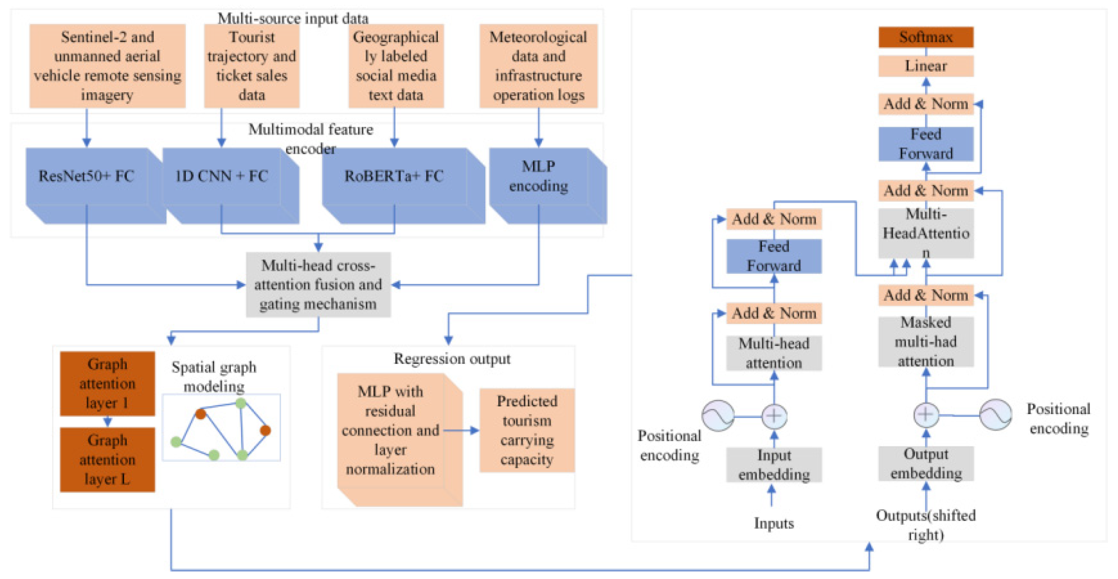
Figure 1. Overall architecture of the forestry tourism resource carrying capacity prediction model.
Forests 17 00534 g001
Figure 2. Spatial map construction.
Forests 17 00534 g002
Figure 3. Comparison of global prediction accuracy and actual prediction curves. (a) Comparison of actual prediction curves for different models; (b) comparison of global prediction accuracy.
Forests 17 00534 g003
Figure 4. Time scale performance. (a) Hourly; (b) daily; (c) seasonal.
Forests 17 00534 g004
Figure 5. Spatial generalization ability analysis. (a) Spatial MAE (GAT-Transformer); (b) spatial MAE (BiLSTM + Transformer); (c) spatial MAE (ARIMA).
Forests 17 00534 g005
Figure 6. Interpretability test of attention weights. (a) Modal attention heatmap (based on node aggregation); (b) GAT edge attention network.
Forests 17 00534 g006
Figure 7. Robustness tests for missing data and noise. (a) RMSE variation under different random mask ratios; (b) RMSE variation under different downsampling intervals; (c) RMSE variation under different cloud coverage ratios.
Forests 17 00534 g007
Table 1. Experimental parameters.
ParameterValueParameterValue
Input modality dimension (trajectory/remote sensing/social media/weather)64/128/32/16Feature-level multi-head attention (modal fusion)Four heads, dim = 128
Temporal window length (input sequence length)24 hNumber of Transformer encoder layersThree floors
Node static feature dimension32Number of Transformer multi-head headsEight heads
Number of GAT layersTwo layersTransformer hidden dimension (model width)256
Number of GAT headsFour heads/layerFFN (in Transformer)1024
GAT hidden dimension (output per layer)128Dropout0.1
GAT edge attention activationLeaky ReLU (0.2)Final regression headTwo-layer fully connected layer
(256 → 64 → 1)
Weight decay1.00 × 10−5Initial learning rate1.00 × 10−4
Gradient clippingGlobal norm1.0Number of training epochs & early stoppingMaximum 200 epochs, early stopping on validation set, patience = 20
Table 2. Ablation analysis of modal contributions.
Modal RemovalMAE (Mean ± Std, Person)ΔMAE (%)RMSE (Mean ± Std, People)ΔRMSE (%)MAPE (Mean ± Std, %)ΔMAPE (%)
Full Modality Removal3.54 ± 0.624.45 ± 0.781.93 ± 0.28
Trajectory Removal5.10 ± 0.95+44.1%6.20 ± 1.10+39.3%2.78 ± 0.42+44.0%
Remote Sensing Removal4.30 ± 0.80+21.5%5.30 ± 0.95+19.1%2.35 ± 0.36+21.8%
Social Media Removal3.95 ± 0.70+11.6%5.05 ± 0.88+13.5%2.20 ± 0.33+14.0%
Weather Removal3.85 ± 0.68+8.8%4.78 ± 0.82+7.4%2.05 ± 0.30+6.2%
Table 3. Computational efficiency and deployability indicators.
ModelParams (M)Size FP32 (MB)Train Time (GPU·h)Inference Latency—CPU (ms)Inference Latency—GPU (ms)
ARIMA0.0010.0040.20.60.2
XGBoost0.050.200.56.01.0
ATT-BiLSTM2.510.0720.03.0
Transformer3.012.0925.04.0
STGCN1.87.2618.02.5
BiLSTM + Transformer4.016.01035.04.5
GCN-LSTM2.811.2722.03.0
GAT-Transformer3.614.41228.03.5
Disclaimer/Publisher’s Note: The statements, opinions and data contained in all publications are solely those of the individual author(s) and contributor(s) and not of MDPI and/or the editor(s). MDPI and/or the editor(s) disclaim responsibility for any injury to people or property resulting from any ideas, methods, instructions or products referred to in the content.