Spatial Imbalance Patterns of Forest Carbon Density and Their Driving Mechanisms in the Xiuhe River Basin

Abstract

Forest carbon sinks are central to climate change mitigation, and prior work has established a solid basis for assessing carbon sinks at regional scales. At the basin scale, however, forest carbon density (vegetation biomass carbon density, i.e., aboveground + belowground biomass carbon; t C ha⁻¹) often shows pronounced spatial clustering and inequality, while its temporal evolution and underlying mechanisms remain poorly quantified and interpreted for management-relevant units such as townships. Using the Xiuhe River Basin as a case study and townships as the basic analytical units, this study identifies the clustered spatial structure and inequality characteristics of forest carbon density and clarifies the joint effects of natural constraints and human disturbances, including potential threshold responses. We first assessed global spatial autocorrelation within a spatial weights framework using Global Moran’s I with permutation tests, and delineated local clustering by classifying local indicators of spatial association (LISA) types based on Local Moran’s I. We then measured the magnitude and stage-wise evolution of inter-township disparities using the Gini coefficient and the Theil T index. Finally, we applied GeoDetector factor, interaction, and risk detection to identify dominant drivers, interaction enhancement, and class-based contrasts. The results show significant and persistent positive spatial autocorrelation in forest carbon density from 2002 to 2024, with Moran’s I ranging from 0.68786 to 0.73849 (p < 0.01). Significant LISA units account for 40.74%–45.37% of townships, and the pattern is dominated by high–high (HH) and low–low (LL) clusters. Inequality follows a stage-wise trajectory: it expanded slightly during 2002–2019, converged markedly during 2019–2021, and rebounded modestly by 2024, while remaining below the levels observed in 2002 and 2019. Strong type-based differentiation is evident in 2024: mean carbon density is 46.06 t C ha⁻¹ in HH areas versus 17.64 t C ha⁻¹ in LL areas; HH areas contribute 38.44% of total carbon stock, whereas LL areas contribute only 5.08%. In terms of drivers, natural and human factors jointly shape the spatial pattern and commonly exhibit interaction enhancement. Elevation (q = 0.7832), slope (q = 0.7133), and NPP (q = 0.6373) are the leading natural constraints, while population density (q = 0.6054) and the built-up land ratio (q = 0.5374) are key indicators of human disturbance. Risk detection further indicates a stable negative gradient for the built-up land ratio and nonlinear class differences for population density, implying that once disturbance intensity reaches higher levels, low-value clustering is more likely to persist. By linking clustered spatial structure, stage-wise inequality, and disturbance-related threshold signals, our results support basin-scale zoning and differentiated management at the township level. Specifically, HH clusters should be prioritized for conservation and connectivity maintenance, whereas LL clusters warrant stricter control of built-up expansion and fragmentation to reduce the risk of persistent low-carbon locking under high disturbance. By linking spatial structure, inequality dynamics, and threshold responses, this study provides a quantitative basis for basin-scale zoning to enhance carbon sinks and for implementing differentiated spatial controls.

1. Introduction

Forest carbon sinks play a pivotal role in the terrestrial carbon budget, and carbon sequestration by terrestrial ecosystems provides an important natural basis for mitigating climate warming [1]. Recent global carbon-budget assessments and key climate indicators show that pressure from fossil-fuel emissions remains pronounced; terrestrial and oceanic sinks buffer the increase in atmospheric greenhouse gases, yet their strength and stability remain uncertain [1,2,3]. Against this background, the sensitivity of forest carbon sinks to extreme climate events and human disturbances has become a core scientific issue for understanding the resilience of natural sinks and for designing feasible policies [4,5,6]. Existing evidence suggests that reducing unnecessary management disturbances and conserving relatively intact forest ecosystems can yield substantial long-term carbon sequestration potential [5,6].

Since China announced its carbon peaking and carbon neutrality goals, the strategic importance of forest carbon sinks has become even more prominent [7,8]. Studies on plantation expansion, optimization of forest management, and pathways to enhance carbon storage indicate that plantation expansion can contribute markedly to carbon gains during certain periods; however, carbon sink capacity is highly heterogeneous in space due to differences in regional ecological conditions, management regimes, and age class structures [9,10,11]. Changes in stand age structure may constrain carbon sink capacity in the short to medium term, thereby affecting the marginal benefits of long-term sequestration targets [1]. In addition, forest carbon dynamics are influenced by a wide range of human activities, including regional economic development, energy consumption, and mitigation policies [12,13]. Therefore, identifying the spatial heterogeneity of forest carbon sinks and their drivers at management-relevant scales such as basins and counties is essential for designing targeted sequestration enhancement and ecological restoration measures.

High-resolution mapping and dynamic monitoring of forest carbon density are prerequisites for identifying and analyzing its spatial heterogeneity [14]. With the increasing availability of multi-source remote sensing data and advances in machine-learning methods, the estimation of aboveground biomass and carbon density has improved substantially in spatial resolution, temporal continuity, and uncertainty characterization [15]. In this study, forest carbon density refers to vegetation biomass carbon density, defined as the sum of aboveground and belowground biomass carbon; soil organic carbon is not included in the carbon calculation. For example, a 30 m annual aboveground biomass dataset for China derived from multi-source remote sensing and deep learning provides critical support for long-term assessments of forest carbon-stock change [16]. A global time series of aboveground biomass inferred from L-band vegetation optical depth offers an important basis for analyzing interannual variability and long-term trends at the global scale [17]. Meanwhile, data-fusion approaches for local to regional applications are also evolving. A deep-learning framework that integrates GEDI LiDAR observations with optical and microwave data has, to some extent, improved the balance between spatial coverage and estimation accuracy [18]. Assessments of GEDI-related error sources, topographic effects, and scale effects indicate that systematic biases may persist under complex terrain and heterogeneous landscapes, calling for targeted methodological improvements and more rigorous validation [19]. Together, these advances enable basin-scale diagnosis of forest carbon density patterns, while also raising the bar for robust indicator processing at management-unit scales and for spatial analyses that account for estimation uncertainty.

Although regional assessments of forest carbon stocks have established a solid foundation, further progress is still needed from the perspective of spatial inequality. First, many studies focus on total changes or mean differences, while paying insufficient attention to the degree of spatial unevenness, clustering forms, and their evolution over time—particularly at the basin scale where spatial polarization and gradient differentiation may reflect the combined effects of physical geographic patterns and human land-use strategies [20,21,22]. Second, driver identification often emphasizes the contribution of single factors, with limited explanation of multi-factor interactions and spatial heterogeneity, which weakens the ability to derive actionable zoning and regulation strategies [23,24]. In recent research on carbon storage and ecosystem services, models such as InVEST and scenario-based simulations have been widely used to evaluate spatial patterns of carbon storage and responses to land-use change, often coupled with GeoDetector (v2018), spatial statistics, and spatial econometric models to interpret the underlying drivers [25,26,27,28]. For instance, a study in arid Northwest China examined how land-use change affects carbon storage and identified spatiotemporal dynamics and spatially varying key drivers [26]. Another study coupled multi-scenario land-use simulation with InVEST and GeoDetector to verify the feasibility of diagnosing driver heterogeneity and assessing policy-scenario impacts at the regional scale [29]. Evidence on urbanization and spatial spillover effects of ecosystem services also suggests that interactions between ecological processes and human activities exhibit strong spatial dependence, and that spatial correlation and spillovers should be explicitly considered in model construction [30]. Consequently, integrating spatial autocorrelation diagnostics, inequality measurement, and driver attribution into a unified framework for basin management units has clear methodological value and practical relevance.

Methodologically, analytical toolkits for detecting spatial stratified heterogeneity and interaction effects have been rapidly advancing in recent years [31]. GeoDetector, a representative approach for spatial stratified heterogeneity, can effectively capture nonlinear relationships and multi-factor interactions and has been widely applied to explain spatial differences in carbon storage, carbon sinks, and ecosystem services. Related software and methodological developments have also been further consolidated in recent years [28]. Methods such as multi-scale geographically weighted regression can reveal how the strength of driver effects varies across space, helping identify dominant factors in different areas [9]. These tools provide technical support for systematic basin-scale analyses and facilitate more coherent arguments regarding the existence of spatial inequality, clustering characteristics, key drivers, and spatial differences in mechanisms.

Using the Xiuhe River Basin as the study area and leveraging multi-period forest carbon density data, this study addresses gaps in the characterization of spatial patterns and mechanism interpretation through three analytical layers. First, within a spatial weights framework, we conduct spatial autocorrelation analysis and local cluster detection to identify clustering characteristics of forest carbon density and their stage-wise changes. Second, we quantify township-level differences and their temporal evolution using the Gini coefficient and the Theil T index to describe spatial inequality. Third, we examine potential drivers from two groups—the natural environment and human activities—by applying GeoDetector to identify key factors and their interactions; risk detection is further used to test differences in carbon density across factor classes. The results provide quantitative evidence to support zoned carbon-sequestration enhancement and differentiated management in the Xiuhe River Basin.

2. Study Area and Data Sources

2.1. Study Area

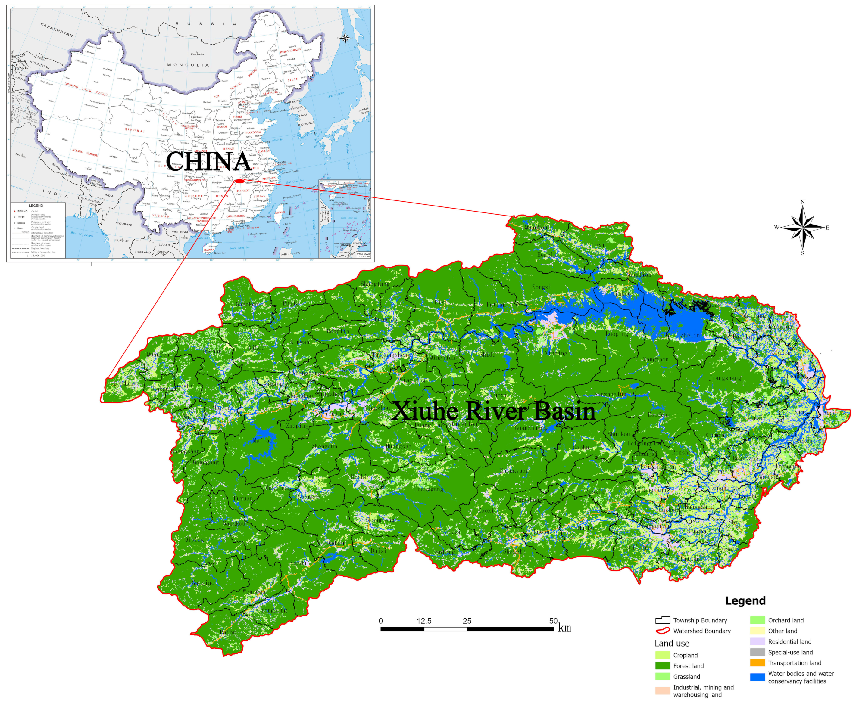
The Xiuhe River Basin (Figure 1) is located in northwestern Jiangxi Province and is one of the five major tributary basins feeding Poyang Lake, the largest freshwater lake in China. The main stem originates from Xiàdòng at Huanglongzhai in the Mufu Mountains. The basin area is about 14,700 km² and covers counties including Yongxiu, Wuning, Xiushui, Jing’an, and Anyi. It accounts for approximately 9.1% of the Poyang Lake Basin. The long-term mean inflow to Poyang Lake is about 14.4 × 10¹⁰ m³, representing roughly 11% of the total inflow from the five major rivers and about 9.4% of the total inflow to Poyang Lake.

In terms of geomorphology, the basin exhibits an upstream mountainous region, a middle reach dominated by rolling hills, and a downstream area characterized by a lacustrine plain interwoven with polder lands. Forestland is mainly distributed across mid-to-high elevation mountains and slopes, whereas towns and cropland are concentrated in valley plains and areas with better transport accessibility. The basin belongs to the subtropical monsoon climate zone; heat and moisture are generally sufficient but unevenly distributed across the year, and the rainy season largely coincides with the vegetation growing season. The Xiuhe River Basin also supports multiple functions, including mountainous water conservation, forest ecological sheltering, and ecological security for the lake region. Forest ecosystems provide foundational services such as soil and water conservation, runoff regulation, and carbon sequestration.

2.2. Data Sources

This study uses townships as the basic spatial analysis units. The data system comprises two parts: contemporary data and extrapolated data. Contemporary data are used to construct explanatory and control variables for 2024, whereas extrapolated data are used to generate the dependent variable—forest carbon density—aligned to the 2024 time baseline. To ensure comparability and reproducibility across multi-source datasets, all spatial data were preprocessed before integration, including clipping to the Xiuhe River Basin extent, unifying coordinate systems, harmonizing raster resolution and alignment, and conducting topology checks and attribute consistency checks for vector data. We also compiled a data inventory and a variable dictionary to document sources, units, processing workflows, and version information.

2.2.1. Contemporary Data

Contemporary data include two groups: natural ecological data and human activity data. Natural ecological data characterize terrain and soil foundations, vegetation growth, and ecological function differences; human activity data represent differences in population concentration, built-up disturbance, industrial emissions, and water environment pressure. The time coverage, data types, and sources of the main datasets are summarized in

Table 1. Data sources used in this study.

No.	Dataset	Time Period	Data Type	Primary Source
1	Xiuhe River Basin boundary and township administrative boundaries	Current version	Vector	Natural resources authorities
2	Land use/land cover map (2024)	2024	Vector	Natural resources authorities
3	Sentinel-2 and Landsat-8 imagery	2024	Raster	Public remote sensing platforms
4	NDVI	2024	Raster	Remote sensing retrieval
5	NPP	2024	Raster	Remote sensing retrieval
6	DEM and terrain derivatives	Latest available	Raster	Natural resources authorities
7	Soil organic matter content	Latest available	Raster or tabular	Natural resources authorities
8	Water conservation importance (ecosystem function assessment output)	2024	Raster	Outputs of ecosystem-function assessment
9	Biodiversity (ecosystem function assessment output)	2024	Raster	Outputs of ecosystem-function assessment
10	Water quality monitoring at sections (monthly and annual mean, 2024)	Monthly and annual mean (2024)	Tabular	Ecology and environment authorities
11	Locations of polluting enterprises and emission data (2024)	2024	Point locations; tabular	Ecology and environment authorities
12	Population and socio-economic statistics (2024)	2024	Tabular	Statistical yearbook
13	Nighttime lights index (2024)	2024	Raster	Public nighttime-lights products
14	Forest carbon density dataset (2002–2021)	2002–2021	Raster	National Tibetan Plateau Data Center [32]

.

Based on the raw datasets listed in Table 1, we further processed multi-source data for 2024 into township-level explanatory and control variables to ensure consistent definitions and traceability for subsequent spatial autocorrelation analysis, inequality measurement, and GeoDetector-based mechanism tests. Variables were grouped into two categories: human activities and natural ecology. The former reflects population concentration, built-up disturbance, economic and industrial activities, and water environment pressure; the latter reflects terrain and soil conditions, vegetation status, and ecological function differences. All variables were derived from the corresponding datasets in Table 1 using zonal statistics, ratio standardization, or density transformations. Townships were used as the accounting units. Raster variables were aggregated primarily by township-level means, while vector and tabular variables were matched to administrative units and normalized by area or population as appropriate. Definitions, units, and brief calculation rules are provided in

Table 2. Variable construction.

Category	Variable (Abbr.)	Unit	Description (Full Name, Data Source, Brief Calculation)
Natural	Elev	m	Elev (elevation). Derived from DEM; aggregated to the township scale using zonal statistics (mean; consistent metric throughout the paper).
	Slope	°	Slope (Slope). Derived from DEM slope raster; aggregated to the township scale using zonal mean (consistent with Elev).
	MAP	mm	MAP (Mean annual precipitation). Based on precipitation raster data; aggregated to township scale using zonal mean.
	SOM	g/kg	SOM (soil organic matter, g/kg). Aggregated to the township scale; raster values use zonal mean, tabular values are joined by township.
	NPP	Product units	NPP (Net primary productivity). Based on NPP raster product; aggregated to township scale using zonal mean.
Human	PopDens	persons/km2	PopDens (population density, persons/km2). Calculated as resident population divided by township area (area from township boundary vectors).
	NTL	Product units	NTL (nighttime light intensity). Based on nighttime-lights raster; aggregated to township scale using zonal mean (consistent metric throughout).
	BuiltRatio	%	BuiltRatio (built-up land ratio, %). Built-up area extracted from the 2024 land-use map; BuiltRatio = built-up area/total township area × 100%.
	RoadDens	km/km2	RoadDens (road density, km/km2). Total road length within each township divided by township area.
	EntDens	firms/km2	EntDens (enterprise density, firms/km2). Number of polluting enterprises within each township divided by township area.

.

2.2.2. Extrapolation of the Dependent Variable

The baseline carbon density data were obtained from the “China forest aboveground and belowground vegetation carbon stock change dataset (2002–2021)”, which provides aboveground vegetation carbon stock (AGBC) and belowground vegetation carbon stock (BGBC) in units of t C ha⁻¹, hosted by the National Tibetan Plateau Data Center. The product provides annual carbon density rasters for each year during 2002–2021; thus, data are available for the full period rather than only for a few selected years reported in the main text. Annual total carbon density rasters at the pixel scale were computed as shown in Equation (1). In this study, TBC denotes total vegetation biomass carbon density, defined as the sum of aboveground and belowground biomass carbon.

$$TBC=AGBC+BGBC$$

(1)

The latest year available in the carbon density product is 2021. To align the dependent variable with explanatory variables for 2024, we used the township-level carbon density series from 2002 to 2021, estimated robust linear trends for each township using the Theil–Sen estimator, and extrapolated these trends to obtain township-level carbon density estimates for 2024. Given the short extrapolation horizon (2021–2024), the linear trend is used as a near-term local approximation for time alignment rather than a long-term growth law.

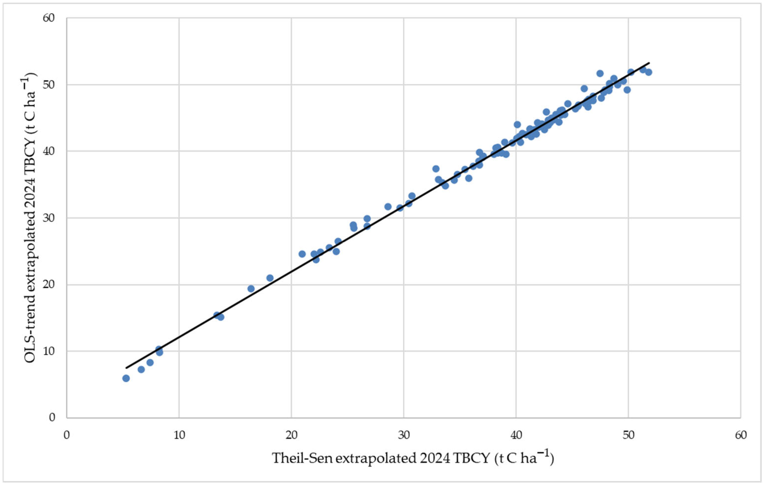
To evaluate the reliability of extrapolation, we conducted hindcast validation: trends were fitted using 2002–2018 as the training period, predictions were generated for 2019–2021, and errors were assessed against corresponding observations. The hindcast sample included 324 township–year records. Results show high consistency between predicted and observed values (R = 0.9803; R² = 0.9610). Overall root mean square error (RMSE) was 3.903 t C ha⁻¹, mean absolute error (MAE) was 3.281 t C ha⁻¹, and mean absolute percentage error (MAPE) was 13.26%. These hindcast metrics provide an empirical uncertainty scale for interpreting short-term interannual variability in the product values. We therefore report 2019–2021 as the most recent observed window and as an empirical variability/validation window that helps contextualize uncertainty around the 2024 extrapolation, while the trend estimation itself is based on the full annual series (2002–2021). Because short-term interannual differences may be influenced by product uncertainty, we interpret the 2019–2021 fluctuations in the context of the hindcast error scale (RMSE/MAE) and report additional paired interannual difference diagnostics in the Appendix. These results indicate that the 2024 carbon density estimates derived from Theil–Sen trend extrapolation have controllable error and are suitable for subsequent analyses of spatial patterns and driving mechanisms. We additionally compared the Theil–Sen-based 2024 estimates with OLS-trend extrapolation and a no-extrapolation 2021 proxy baseline; the consistency diagnostics are reported in Appendix A 

Table A4. Sensitivity comparison of township-level 2024 carbon density estimates under alternative extrapolation settings.

Comparison	Pearson r	Spearman ρ	MAD (t C ha−1)	RMSE (t C ha−1)	Top-Decile Overlap	Bottom-Decile Overlap
Theil–Sen 2024 vs. OLS-trend 2024	0.997	0.993	1.733	1.932	0.818	0.909
Theil–Sen 2024 vs. 2021 proxy baseline	0.985	0.973	1.413	1.985	0.636	0.909

and Figure A1. We additionally assessed whether the hindcast uncertainty is spatially heterogeneous along a terrain gradient using township mean elevation, as reported in Appendix A and

Table A5. Terrain-stratified hindcast error statistics for 2019–2021 and association with elevation.

Elevation Class	MAE (t C ha−1)	RMSE (t C ha−1)	MAPE (%)
T1 (lowest)	3.53	4.331	20.79
T2	2.238	2.827	6.069
T3 (highest)	2.307	2.812	5.239
All (pooled)	2.691	3.399	10.699
T1 (lowest)	3.53	4.331	20.79

.

3. Methods

We constructed a township-level forest carbon density indicator system and conducted pattern identification, inequality quantification, and mechanism analysis within a unified spatial-analytical framework. For pattern identification, we applied Global Moran’s I with permutation tests to assess overall spatial autocorrelation in forest carbon density, and then used Local Moran’s I to detect local high–high clusters, low–low clusters, and spatial outliers, thereby characterizing the clustering structure and its spatial boundaries. Spatial association was assessed using a global-to-local workflow under a consistent spatial weights specification: Global Moran’s I summarizes the overall clustering tendency, while Local Moran’s I (LISA) maps local clusters and spatial outliers. Alternative statistics (e.g., Geary’s C or Getis-Ord Gi) provide complementary views of spatial association, but the Moran/LISA combination is sufficient for the pattern description and mapping tasks in this study. Spatial relationships among townships were represented by a contiguity-based spatial weights matrix (W). Specifically, we constructed W as a first-order contiguity matrix, where $w_{ij}=1$ if townships i and j share a common boundary (and $w_{ij}=0$ otherwise). To account for heterogeneous numbers of neighbors caused by irregular administrative boundaries, we applied row-standardization so that the weights in each row sum to one (${{\displaystyle \sum }}_j{w}_{ij}=1$). The same W was used consistently for Global Moran’s I and Local Moran’s I (LISA). A sensitivity check using an alternative spatial weights specification was conducted and is documented in

Table B1. Spatial weights robustness results under rook and kNN.

Year	Weights	Global Moran’s I	p-Value
2002	Rook (baseline)	0.68786	p < 0.001
2002	kNN (k = 6)	0.61269	p < 0.001
2019	Rook (baseline)	0.73849	p < 0.001
2019	kNN (k = 6)	0.67198	p < 0.001
2020	Rook (baseline)	0.72464	p < 0.001
2020	kNN (k = 6)	0.65304	p < 0.001
2021	Rook (baseline)	0.69515	p < 0.001
2021	kNN (k = 6)	0.64154	p < 0.001
2024	Rook (baseline)	0.73138	p < 0.001
2024	kNN (k = 6)	0.67533	p < 0.001

. For inequality measurement, we employed the Gini coefficient and the Theil T index to quantify the level of township-level differences and their stage-wise changes. For associated-factor analysis, we examined two groups of explanatory variables—natural environment and human activities—using GeoDetector, including factor detection, interaction detection, and risk detection, to evaluate single-factor explanatory power, test interaction enhancement effects, and compare mean differences in carbon density across factor classes. GeoDetector is used here to quantify spatially stratified heterogeneity and explanatory association (q-statistic) rather than to identify causal effects; therefore, “drivers/mechanisms” are interpreted as dominant associated factors and interaction patterns. Core formulas, parameter definitions, and key references are provided in

Table 3. Summary of analytical methods.

Method Module	Purpose	Formula	Explanation (Parameter Definitions)	References
Forest carbon density indicator	Construct the dependent variable at the township scale to obtain a comparable carbon density series	$FC{D}_i={\displaystyle \frac{F{C}_i}{A_i}}$	$FC{D}_i$ is forest carbon density for township $i$; $F{C}_i$ is total forest carbon stock within forestland in township i; $A_i$ is forestland area in township i. To reduce volatility in very small forest areas, report the forestland-area threshold and the harmonized handling rule.	[33,34]
Global spatial autocorrelation (Global Moran’s I)	Test overall spatial dependence and clustering	$I={\displaystyle \frac{n}{S_0}}{\displaystyle \frac{{\displaystyle \sum _i{\displaystyle \sum _j{w}_{ij}}}(x_i-\overline{x})(x_j-\overline{x})}{{\displaystyle \sum _i{(x_i-\overline{x})}^2}}}$	$n$ is the number of townships; $x_i$ is carbon density in township $i$; $\overline{x}$ is the mean; $w_{ij}$ is the element of the spatial weights matrix reflecting neighborhood relation/strength between $i$ and $j$; $S_0={\displaystyle \sum _i{\displaystyle \sum _j{w}_{ij}}}$ is the sum of weights used for normalization. Significance is assessed via permutation tests with 9999 permutations (two-sided).	[35,36]
Local spatial autocorrelation (LISA/Local Moran’s I)	Identify HH/LL clusters and spatial outliers	$I_i={\displaystyle \frac{(x_i-\overline{x})}{m^2}}{\displaystyle \sum _j{w}_{ij}}(x_j-\overline{x})$	$I_i$ is the local autocorrelation statistic for township $i$; definitions of $x_i,\overline{x}$, and $w_{ij}$ follow above; $m^2={\displaystyle \frac{1}{n}}{\displaystyle \sum _i{(x_i-\overline{x})}^2}$ is the sample variance (or equivalent scaling factor) for standardization. HH/LL/HL/LH are determined by the sign of $I_i$ and the direction of neighborhood mean; significance is assessed via permutation tests with 9999 permutations (two-sided), and local units are considered significant at p ≤ 0.05.	[37,38,39]
Inequality measurement (Theil T)	Quantify township-level inequality and its stage-wise changes	$T={\displaystyle \frac{1}{n}}{\displaystyle \sum _i\raisebox{1ex}{$x_i$}\!\left/ \!\raisebox{-1ex}{$\overline{x}$}\right.}\ln \left({\displaystyle \raisebox{1ex}{$x_i$}\!\left/ \!\raisebox{-1ex}{$\overline{x}$}\right.}\right)$	$T$ is the overall Theil index; $x_i$ is carbon density for township $i$; $\overline{x}$ is the mean; $n$ is the number of townships. The term (${\displaystyle \raisebox{1ex}{$x_i$}\!\left/ \!\raisebox{-1ex}{$\overline{x}$}\right.}$) captures relative level and $\ln (\cdot )$ reflects inequality on a log scale. If group decomposition is used, report grouping criteria and within-/between-group aggregation rules.	[40,41]
GeoDetector: attribution of spatial differentiation and interaction tests	Quantify explanatory power of drivers and test interaction enhancement	$q=1-{\displaystyle \frac{{\displaystyle \sum _h{N}_h}{\sigma }_h^2}{N{\sigma }^2}}$	$q$ is the explanatory-power statistic (larger $q$ indicates stronger explanation of spatial differentiation); $h$ indexes strata (classes); $N_h$ is the number of townships in stratum $h$; ${\sigma }_h^2$ is the variance of carbon density within stratum $h$; $N$ is the total sample size; ${\sigma }^2$ is the overall variance. Interaction detection compares $q$ of the overlay of two factors with $q$ of each single factor to classify enhancement types. Report the discretization method and the number of strata for continuous variables.	[42,43,44]

Note: FCD, forest carbon density; HH, high–high cluster; LL, low–low cluster; HL, high–low outlier; LH, low–high outlier.

.

4. Results

4.1. Spatial Distribution of Forest Carbon Density

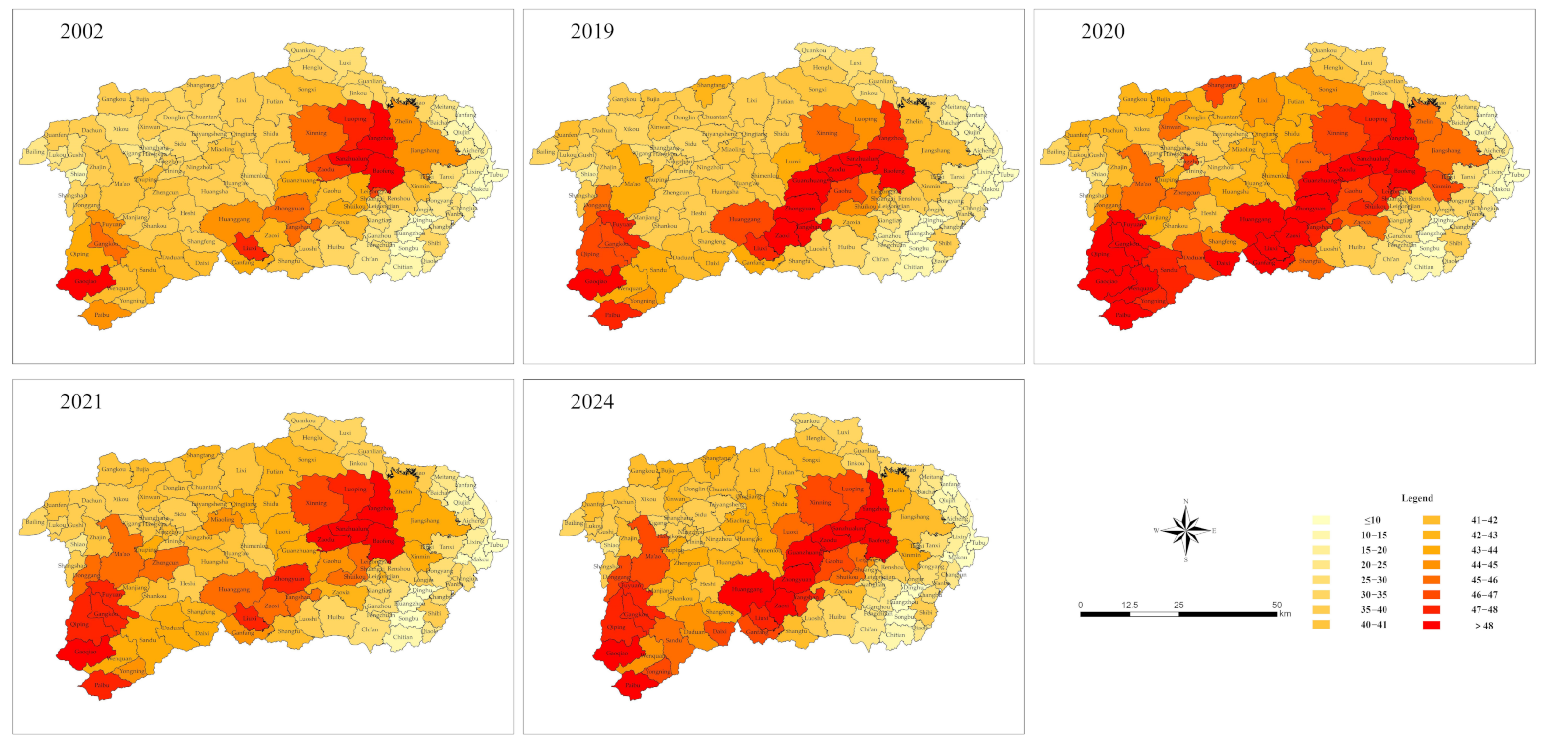
Based on township-level mean forest carbon density data, the Xiuhe River Basin exhibits a stable spatial differentiation pattern alongside stage-wise temporal fluctuations across 2002, 2019, 2020, 2021, and 2024 (

Table 4. Descriptive statistics of township-level forest carbon density in the Xiuhe River Basin.

Year	Mean (t C ha−1)	SD (t C ha−1)	CV	Min (t C ha−1)	Max (t C ha−1)
2002	33.65	11.20	0.33	2.66	53.09
2019	34.75	11.87	0.34	3.76	51.93
2020	38.35	11.87	0.31	4.44	56.2
2021	36.88	10.96	0.30	4.78	50.46
2024	37.06	11.44	0.31	5.28	51.8

Note: Values for 2024 are extrapolated from historical series; statistics are computed at the township level. SD, standard deviation; CV, coefficient of variation.

; Figure 2). Township-level forest carbon density is derived from forest land only. Non-forest areas are excluded using a forest mask, and the results are aggregated to the township unit for mapping and subsequent analysis in units of t C ha⁻¹. Overall, township-level differences are substantial: mean carbon density was 33.83 t C ha⁻¹ in 2002 and 34.88 t C ha⁻¹ in 2019; it increased to 38.48 t C ha⁻¹ in 2020, declined to 36.97 t C ha⁻¹ in 2021, and reached 37.16 t C ha⁻¹ in 2024. These results indicate an overall upward trend with notable short-term fluctuations. Spatially, carbon density shows a persistent unequal pattern: contiguous high-value areas are mainly located in the central to southwestern basin, whereas low-value depressions are concentrated along the eastern basin margin and in some more urbanized areas. This pattern is summarized in Figure 3. Township-level forest carbon density represents the mean carbon density of forest land within each township rather than forest-cover extent. All subsequent analyses in this study use the township-level mean forest carbon density as the input variable.

Figure 2. Spatial distribution of township-level mean forest carbon density on forest land in the Xiuhe River Basin (Unit: t C ha⁻¹).

Figure 2. Spatial distribution of township-level mean forest carbon density on forest land in the Xiuhe River Basin (Unit: t C ha⁻¹).

Notes: Values are township-level means aggregated from forest pixels only; non-forest areas are excluded by a forest mask.

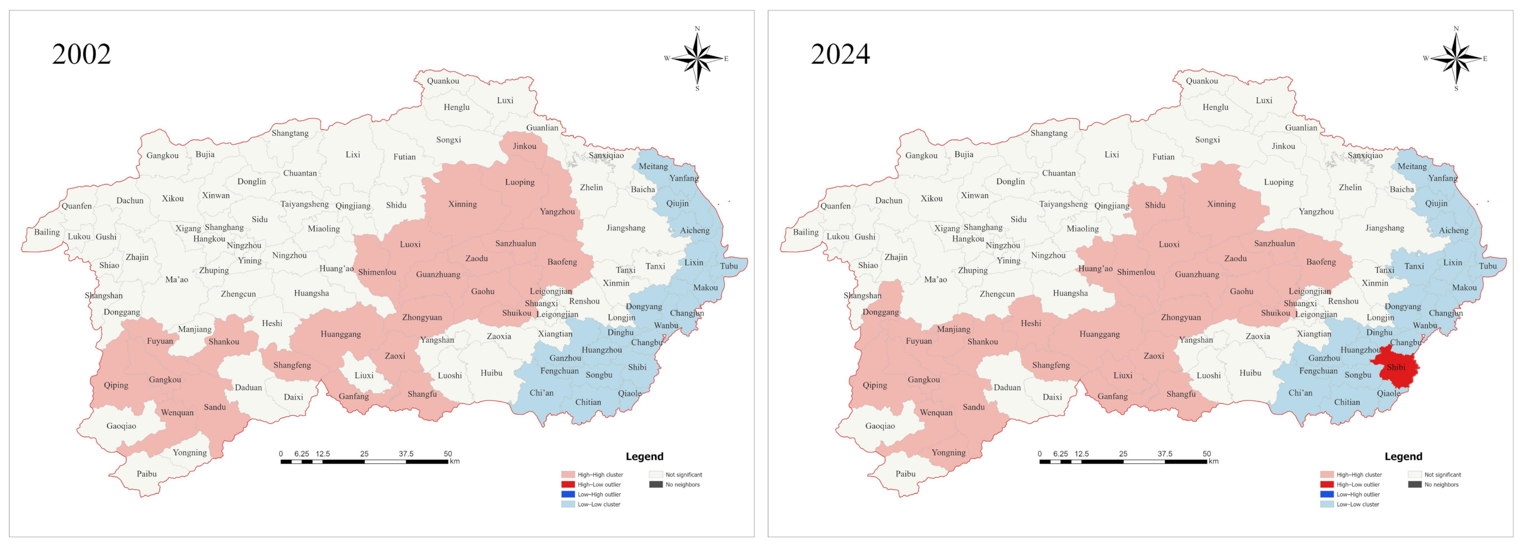
Figure 3. LISA cluster/outlier patterns of township-level forest carbon density in the Xiuhe River Basin.

Figure 3. LISA cluster/outlier patterns of township-level forest carbon density in the Xiuhe River Basin.

4.2. Spatial Autocorrelation and Clustering Structure

To analyze spatial inequality in forest carbon density, we tested spatial dependence and structural forms at both global and local levels. Globally, Global Moran’s I values for 2002, 2019, 2020, 2021, and 2024 are all significantly positive (I = 0.68786–0.73849; Z = 9.43732–10.12056; p < 0.01;

Table 5. Global Moran’s I of township-level forest carbon density in the Xiuhe River Basin.

Year	Moran’s I	Z-Score	p-Value	Significance
2002	0.68786	9.43732	p < 0.01	Significant positive autocorrelation
2019	0.73849	10.12056	p < 0.01	Significant positive autocorrelation
2020	0.72464	9.96909	p < 0.01	Significant positive autocorrelation
2021	0.69515	9.59013	p < 0.01	Significant positive autocorrelation
2024	0.73138	10.05323	p < 0.01	Significant positive autocorrelation

Note: Z-scores and p-values are based on a permutation test with 9999 permutations (two-sided).

), indicating that forest carbon distribution in each period significantly deviates from a spatially random process and exhibits strong positive spatial autocorrelation. This implies a stable clustered structure of spatial inequality at the basin scale—high values tend to be adjacent to high values, and low values tend to be adjacent to low values.

We used Anselin Local Moran’s I to classify local spatial association types and summarized the composition of significant units (

Table 6. Counts of LISA cluster types and the share of significant units.

Year	HH	LL	HL	LH	Share of Significant Units
2002	24	20	0	0	40.74%
2019	26	19	1	0	42.59%
2020	25	20	0	0	41.67%
2021	26	20	1	1	44.44%
2024	28	20	1	0	45.37%

Note: HH and LL denote high–high contiguous areas and low–low depressions, respectively; HL and LH denote spatial outliers. The share of significant units is the proportion of townships that pass the significance test. Local Moran’s I significance is assessed using 9999 permutations (two-sided) with p ≤ 0.05

). Across the study period, the share of significant units ranges from 40.74% to 45.37% and shows an overall increasing tendency, suggesting that the clustering structure did not weaken as overall carbon density increased; rather, it became somewhat stronger. In terms of type composition, significant units are almost entirely dominated by like-value cluster types. High–high clusters (HH) and low–low clusters (LL) account for the vast majority of significant units: in 2002, HH and LL counts were 24 and 20, respectively, while HL and LH were both zero. During 2019–2024, only a very small number of outlier types appeared (HL ≤ 1; LH ≤ 1), without altering the overall structural interpretation. This indicates that spatial inequality in the basin is primarily characterized by clustered differentiation, whereas spatial mismatch (outlier patterns) is generally weak.

The robustness check using the alternative kNN weights (k = 6) yields the same qualitative inference as the baseline rook specification: Global Moran’s I remains significantly positive for 2002, 2019–2021, and 2024. Therefore, the conclusion of basin-scale positive spatial autocorrelation is not sensitive to the spatial weights specification (Table B1).

To visualize the directional pattern and stability of clustering, we selected 2002 and 2024 as representative years and mapped LISA clusters (Figure 3). Both years exhibit a clear bipolar clustering pattern. HH areas show strong continuity and connectivity, whereas LL areas form a relatively stable low-value belt along the basin margin. The clustering intensity of HH areas tends to strengthen, while LL areas display pronounced structural stability. Meanwhile, only one HL unit appears in 2024, and LH equals zero, further indicating that the basin-wide pattern remains dominated by like-value clustering.

4.3. Measuring Inequality and Its Temporal Evolution

To further quantify spatial inequality in forest carbon density, we used the Gini coefficient and the Theil T index to measure township-level differences and their stage-wise changes, thereby revealing expansion and convergence of inequality over the study period.

Overall inequality metrics indicate a clear stage-wise trajectory. The Gini coefficients in 2002 and 2019 were 0.179 and 0.181, and the Theil T indices were 0.066 and 0.070, respectively, indicating a slight increase in inequality from 2002 to 2019. After 2019, inequality converged markedly: in 2021 the Gini declined to 0.149 and the Theil T index to 0.054, representing a stage-wise low. By 2024, the Gini rose to 0.159 and the Theil T index to 0.058. Although there is some rebound, both values remain below the corresponding levels in 2002 and 2019 (

Table 7. Inequality metrics of township-level forest carbon density in the Xiuhe River Basin.

Year	Mean	SD	CV	Gini	Theil T	Min	Max
2002	33.825	11.159	0.330	0.179	0.066	2.664	53.086
2019	34.877	11.771	0.338	0.181	0.070	3.757	51.929
2020	38.480	11.772	0.306	0.160	0.058	4.437	56.202
2021	36.967	10.835	0.293	0.149	0.054	4.775	50.46
2024	37.159	11.317	0.305	0.159	0.058	5.281	51.795

). These results suggest that township-level differences persist over the long term, but their intensity is not monotonic; instead, it undergoes stage-wise adjustments between expansion and convergence.

4.4. Driver Analysis

To assess the relative contributions of natural background and human activities to spatial inequality, we applied GeoDetector to analyze the relationships between township-level forest carbon density (2024) and potential drivers using factor detection, interaction detection, and risk detection. Drivers include terrain conditions (Elev, Slope), climatic background (MAP), soil conditions (SOM, 0–30 cm), vegetation productivity (NPP), and indicators of human activity intensity (PopDens, NTL, BuiltRatio, RoadDens, EntDens).

All factors pass significance tests and show clear gradients in explanatory power. Among natural factors, Elev has the strongest explanatory power (q = 0.7832), followed by Slope (q = 0.7133); NPP also shows strong explanatory power (q = 0.6373), indicating that terrain constraints and productivity differences provide a fundamental basis for spatial differentiation in forest carbon. Among human activity factors, PopDens (q = 0.6054) and BuiltRatio (q = 0.5374) show relatively high explanatory power, indicating strong spatially stratified associations between development intensity/population concentration and the spatial differentiation of forest carbon density (

Table 8. GeoDetector factor detector results.

Factor	q Statistic	p Value
Elev	0.7832	p < 0.001
Slope	0.7133	p < 0.001
MAP	0.2074	p < 0.001
SOM (g/kg)	0.1100	0.037
NPP	0.6373	p < 0.001
PopDens (person/km2)	0.6054	p < 0.001
NTL	0.2899	p < 0.001
BuiltRatio (%)	0.5374	p < 0.001
RoadDens (km/km2)	0.2577	p < 0.001
EntDens (per/km2)	0.1812	p < 0.001

).

Interaction detection (

Table 9. Highest-explaining interaction pairs from GeoDetector.

Factor Pair	q (Interaction)	Type
Elev × RoadDens	0.8509	Bivariate enhancement
Elev × MAP	0.8497	Bivariate enhancement
Elev × PopDens	0.8429	Bivariate enhancement
Elev × NTL	0.8386	Bivariate enhancement
Elev × NPP	0.8376	Bivariate enhancement
Elev × BuiltRatio	0.8371	Bivariate enhancement
Slope × RoadDens	0.8127	Bivariate enhancement
Elev × Slope	0.8110	Bivariate enhancement
Elev × SOM	0.8040	Bivariate enhancement
Elev × EntDens	0.8032	Bivariate enhancement

) shows that the combined effects of multiple factors substantially enhance explanatory power for spatial differences in forest carbon. These interaction patterns indicate that the explanatory association for forest-carbon spatial differentiation is stronger when factors are considered jointly, consistent with GeoDetector’s interaction detection classification. The strongest interactions are largely associated with Elev combined with other factors, such as Elev × RoadDens (q = 0.8509), Elev × MAP (q = 0.8497), and Elev × PopDens (q = 0.8429), showing that elevation jointly with human activity and climatic factors yields a higher explanatory association than single factors alone.

Based on equal-interval discretization consistent with the above analyses, we further conducted risk detection to test differences in mean carbon density across factor classes. Key factors exhibit clear gradients across five classes. Elev and NPP show stable positive gradients: as class increases from 1 to 5, mean carbon density rises from 20.10 to 49.26 t C ha⁻¹ for Elev, and from 20.25 to 48.81 t C ha⁻¹ for NPP. BuiltRatio shows a pronounced negative gradient, with mean carbon density decreasing from 47.78 to 25.16 t C ha⁻¹. PopDens exhibits a nonlinear response: low to middle classes correspond to relatively higher carbon density, whereas the highest class shows a marked decrease, implying potential threshold amplification associated with population agglomeration (

Table 10. GeoDetector risk detector results for key factors (t C ha⁻¹).

Factor	Sample Size by Class (n)	Class 1	Class 2	Class 3	Class 4	Class 5
Elev	21/21/21/21/20	20.10	34.62	44.12	45.35	49.26
NPP	21/21/21/21/20	20.25	35.61	42.89	45.87	48.81
PopDens	21/21/21/21/20	47.09	44.66	45.50	26.54	28.68
BuiltRatio	21/21/21/21/20	47.78	44.29	40.65	34.42	25.16

). Risk detection thus complements factor detection from an interval-comparison perspective and provides more intuitive gradient evidence for interpreting mechanism differences across LISA types.

4.5. Heterogeneity in Driving Mechanisms Across LISA Types

To reveal mechanism heterogeneity across spatial clustering types, we used Local Moran’s I-based LISA types as grouping criteria and classified townships into HH (high–high clusters), LL (low–low clusters), and NS (not significant). We then conducted between-group comparisons within this framework. Combined with GeoDetector factor and interaction results, we compared how natural constraints and human disturbances differ across types in their explanatory power and interaction enhancement, thereby linking “spatial clustering patterns” and “driving mechanisms” at the same analytical unit.

LISA results indicate stable HH and LL areas in the Xiuhe River Basin. Structurally, there were 24 HH and 20 LL units in 2002; by 2024, HH increased to 28 while LL remained at 20, suggesting some expansion of high-value clusters and strong locking of low-value clusters. To interpret these differences mechanistically, we focus on 2024 and compare systematic differences among HH, LL, and NS units in carbon density levels, forestland scale, and key drivers, cross-checking with GeoDetector factor and interaction results from Section 4.4 (

Table 11. Forestland scale and carbon contribution across LISA types in 2024.

Type	n	Total Forestland Area (km2)	Share of Forestland Area (%)	Mean Carbon Density, 2024 (t C ha−1)	SD	Total Carbon Stock (t C)	Share of Carbon Stock (%)
HH	28	4739.73	33.31	46.06	2.94	21,867,601	38.44
LL	20	1639.23	11.52	17.64	8.45	2,889,769	5.08
HL	1	94.38	0.66	38.04		359,011	0.63
NS	59	7754.41	54.5	39.54	5.79	31,776,514	55.85

).

Driver differences between HH and LL show opposing patterns between natural constraints and human activity intensity. HH units have significantly higher Elev, Slope, and NPP, whereas LL units have significantly higher PopDens, BuiltRatio, RoadDens, nighttime lights, and enterprise density (

Table 12. Differences in key drivers among HH, LL, and NS types in 2024.

Indicator	HH (n = 28)	LL (n = 20)	NS (n = 57)	p-Value (HH vs. LL)
Elev (m)	499.88 ± 140.24	59.57 ± 16.55	297.68 ± 147.42	<0.001
Slope (°)	16.02 ± 2.51	1.16 ± 1.40	10.91 ± 4.70	<0.001
NPP	2976.67 ± 107.06	2283.71 ± 190.60	2786.84 ± 240.29	<0.001
MAP (mm)	1673.61 ± 57.12	1597.17 ± 47.34	1627.30 ± 52.94	<0.001
Organic matter (g/kg)	2.63 ± 0.93	1.99 ± 0.59	2.43 ± 1.16	0.012
PopDens (person/km2)	94.77 ± 69.16	517.95 ± 648.09	247.30 ± 353.48	<0.001
BuiltRatio (%)	2.37 ± 1.62	12.29 ± 6.12	4.53 ± 4.54	<0.001
RoadDens (km/km2)	0.338 ± 0.126	0.596 ± 0.166	0.370 ± 0.152	<0.001
NTL	0.763 ± 0.864	1.754 ± 2.026	0.853 ± 0.980	<0.001
EntDens (per/km2)	0.139 ± 0.179	0.617 ± 1.068	0.190 ± 0.284	<0.001

). These type-wise contrasts corroborate the GeoDetector rankings: Elev, Slope, and NPP are the strongest natural drivers, while PopDens and BuiltRatio are among the most influential human activity drivers. Moreover, interaction detection shows enhancement effects for Elev combined with RoadDens, PopDens, and BuiltRatio, implying that natural background not only affects carbon density directly but also amplifies the influence of human disturbances. Together with risk detection, the stable negative gradient of BuiltRatio and the pronounced nonlinear class differences in PopDens further support the interpretation that LL clustering is likely associated with threshold effects once development intensity reaches higher classes, while HH clustering is maintained by the combined support of favorable natural conditions and lower disturbance intensity. Therefore, spatial inequality in the basin reflects differentiated coupled mechanisms across types: HH corresponds more to “high-value clustering supported by terrain and productivity”, whereas LL corresponds more to “low-value locking driven by intensive human activities”.

5. Discussion

5.1. The Non-Random Nature of Spatial Clustering in Basin-Scale Forest Carbon Density

At the township scale, we observe significant positive spatial autocorrelation in forest carbon density for 2002, 2019, 2020, 2021, and 2024 (Moran’s I = 0.68786–0.73849; Z > 9; p < 0.01). LISA types are dominated by HH and LL, and the share of significant units is about 40.74%–45.37%. This indicates that forest carbon density in the Xiuhe River Basin is not independently distributed; instead, it is organized by discernible spatial processes with homogeneous clustering and spatial dependence among neighboring units. Similar clustering patterns are widely reported in international studies of forest carbon and related carbon-pool variables, often attributed to the combined effects of terrain background, vegetation productivity, stand succession, and management activities that generate spatial continuity and diffusion-like effects. In subtropical regions, previous studies have also used Global and Local Moran’s I to identify significant spatial autocorrelation and hotspot–coldspot structures in forest carbon density, providing external consistency for our spatial-statistical findings. This is consistent with a common empirical pattern reported in forest carbon studies, where carbon- and biomass-related variables show clear spatial dependence and clustering, and Global/Local Moran’s I are routinely used to diagnose overall dependence and local clusters/outliers and to link non-random distributions to underlying spatial processes [18,45].

Mechanistically, spatial autocorrelation is more than a statistical feature; it implies neighborhood effects and spatial propagation in carbon density differences. Treating townships as independent samples may therefore underestimate the contribution of spatial processes to inequality formation. This is why we begin the analytical chain with global tests and local-cluster identification under a spatial weights framework, consistent with common workflows in spatial ecology.

5.2. Stage-Wise Evolution of Inequality and Its Structural Sources

Inequality metrics indicate that differences slightly widened during 2002–2019, converged markedly during 2019–2021, and rebounded modestly by 2024, while remaining below the levels observed in 2002 and 2019. This stage-wise trajectory suggests, first, that changes in differences are unlikely to be a simple monotonic increase or decrease; rather, they may reflect period-specific reallocations in carbon accumulation rates across subregions. Second, short-term convergence does not imply the disappearance of spatial differences. Because the clustering structure remains significant, convergence more likely reflects a change in the amplitude between high and low values rather than a breakdown of the clustering structure.

International evidence reaches similar conclusions: temporal changes in forest-carbon patterns are often jointly driven by natural disturbances, adjustments in management strategies, land-use change, and interannual climate variability, which can desynchronize carbon density change rates across regions and lead to stage-wise expansion or convergence of differences. Accordingly, our stage-wise findings should be interpreted together with spatial-structure results: variation in inequality metrics is, to a large extent, constrained by both the stability and possible expansion of HH and LL types rather than by uniform basin-wide change. This interpretation matches the broader view that inequality trajectories often reflect period-specific reallocations in growth rates across subregions under jointly varying disturbance, management, and climate signals, rather than uniform basin-wide change.

5.3. Type-Wise Structural Differentiation and an Explanation for Unequal Carbon Contributions

In 2024, mean carbon density in HH areas (46.06 t C ha⁻¹) is far higher than that in LL areas (17.64 t C ha⁻¹), and this difference translates into an unequal contribution structure: HH areas account for 33.31% of forestland area but contribute 38.44% of total carbon stock, whereas LL areas account for 11.52% of forestland area but contribute only 5.08%. The key implication is that spatial inequality is not merely a matter of mean differences; it is also a problem of “unequal contribution structure” driven by differentiation among LISA types. In other words, HH is not only a high-value region but also a high-contribution region, while LL is not only a low-value region but also a low-contribution cluster that structurally constrains overall carbon-sink efficiency. This interpretation aligns with a broad international understanding that high-biomass or high-carbon-density regions often carry disproportionate shares of carbon stocks, whereas low-value clusters are frequently associated with fragmentation and intensified human disturbance, forming persistent low-carbon constraint belts. This mainstream evidence also emphasizes mechanism-relevant links: low-value clusters are often coupled with fragmentation and edge effects under intense human disturbance, and built-up encroachment tends to reduce ecosystem carbon storage, with edge-driven biomass losses becoming more pronounced in fragmented forests [46,47,48].

Moreover, HH counts increase over the study period while LL remains stable, indicating that structural differentiation is not static: high-value clusters may expand or strengthen in contiguity, whereas low-value locked areas show notable persistence. From an interpretive (association-based) perspective, these patterns are consistent with the co-occurrence of favorable natural backgrounds and protection/management in high-value areas, whereas low-value areas tend to coincide with more intensive human activity contexts.

5.4. Coupled Effects of Natural Constraints and Human Disturbances and Their Interaction Enhancement

GeoDetector factor detection indicates that Elev (q = 0.7832) and Slope (q = 0.7133) have the strongest explanatory power, with NPP (q = 0.6373) also contributing substantially. Among human activity factors, PopDens (q = 0.6054) and BuiltRatio (q = 0.5374) stand out. This ranking suggests that spatial differences in forest carbon density in the Xiuhe River Basin are anchored in natural background constraints and are strongly modulated by human activity intensity. GeoDetector’s underlying concept of spatial stratified heterogeneity and the q statistic have been well developed in methodological literature and widely applied in ecological and environmental attribution, making the framework appropriate for nonlinearity and interaction effects and internationally comparable.

More importantly, interaction detection shows that most factor combinations exhibit enhancement effects. This implies that natural conditions do not merely provide background differences; they can also reshape how human activities manifest spatially, producing interaction amplification in a statistical sense. Global evidence has shown consistent declines in forest carbon along gradients of human degradation even after controlling for climate and soil conditions, indicating a stable negative effect of human disturbance on carbon density across regions. Our results—significant explanatory power for human activity indicators and their enhanced interactions with natural factors—are consistent with this direction and mechanism logic. This is in line with a widely reported attribution pattern: terrain and productivity act as primary natural constraints on forest carbon/biomass, while human activity proxies such as population density, nighttime lights, and built-up land exert significant influences and often interact with natural factors in enhancement or nonlinear ways [3,49,50]. Because the analysis is based on cross-sectional spatial association and GeoDetector’s explanatory attribution, the identified factors and interactions should be interpreted as statistical associations rather than causal mechanisms; causal identification would require additional designs (e.g., longitudinal data, quasi-experiments, or explicit causal-inference frameworks).

5.5. Threshold Responses and the Formation Mechanism of Low-Value Locking

Risk detection indicates a stable negative gradient response for BuiltRatio and a nonlinear class response for PopDens, suggesting threshold effects of human disturbance intensity. Ecologically, once built-up expansion and population agglomeration reach certain intensity levels, forestland fragmentation, edge effects, and microclimatic changes are more likely to be persistently triggered, amplifying declines in carbon density and forming spatially locked LL low-value clusters. International studies have quantified substantial reductions in forest aboveground biomass attributable to edge effects at the global scale and emphasized that fragmentation should be explicitly incorporated into carbon accounting and assessment frameworks, providing a strong external evidence chain supporting our interpretation of thresholds and low-value locking. More broadly, studies on spatial heterogeneity commonly report interaction enhancement under multi-factor coupling and identify disturbance-related thresholds or threshold intervals that can trigger nonlinear shifts and persistence in carbon stocks or sinks, which provides a direct parallel to the threshold signals observed here and supports zoned management implications [50,51,52].

Based on this evidence chain, the core academic contribution of this study can be summarized as a mechanism pathway: a clustered spatial structure provides the precondition; type-wise structural differentiation constitutes the structural source of inequality; natural constraints and human disturbances jointly drive inequality and amplify differences through interaction enhancement; and threshold responses further explain the stable locking of low-value clusters. This pathway elevates the study from descriptive patterns to testable mechanism inference and offers direct scientific support for zoned management.

To examine whether the above mechanism interpretation is consistent with broader evidence—and to avoid idiosyncratic inference based on a single study area—we further benchmark our key findings against relatively stable conclusions in international literature. The comparison addresses four aspects: whether clustered spatial structures are widely observed; whether inequality exhibits clear structural characteristics; whether the relative importance ranking of natural constraints versus human disturbances is consistent; and whether multi-factor interactions and threshold responses can explain the stability of low-value clusters. This benchmarking is not intended to replace the statistical tests above; rather, it provides external evidence to validate interpretability and generalizability, thereby strengthening the credibility of mechanism inference and zoning implications.

5.6. Limitations and Future Directions

It should be noted that this study is subject to methodological constraints that may influence result interpretation. The 2024 forest carbon density was derived by extrapolating township-level trends over 2002–2021 using the Theil–Sen estimator; while the hindcast validation indicates acceptable performance, abrupt shocks or nonlinear changes after 2021 may not be fully captured. The hindcast diagnostics further suggest modest terrain-related uncertainty heterogeneity, with comparatively larger errors in lower-elevation townships, and we therefore interpret short-term fluctuations more cautiously for that group. In addition, the dependent variable represents vegetation biomass carbon density from the adopted product and does not constitute a complete ecosystem carbon budget that would incorporate deadwood, litter, and soil organic carbon pools. Finally, the spatial-diagnostic and attribution outcomes may be sensitive to key analytical settings, including township aggregation (MAUP), the specification of spatial weights for Moran’s I/LISA, and discretization schemes in GeoDetector, which can affect clustering delineation, q values, and interaction classification. Edge effects are also a common concern in areal spatial statistics because boundary townships typically have fewer potential neighbors within the study window, which may influence spatial-lag calculations and the identification of local clusters/outliers near the perimeter. In this study, the contiguity-based weights matrix was row-standardized, which helps reduce sensitivity to heterogeneous neighbor counts by placing each township’s spatial lag on a comparable scale; nevertheless, spatial patterns detected close to the boundary should be interpreted with caution.

Future work will focus on extending carbon density products beyond 2021 or integrating change-detection constraints and on conducting systematic sensitivity and uncertainty analyses across spatial units and parameter choices. In particular, incorporating buffer zones or external neighboring units when compatible data are available may further mitigate edge effects in boundary areas.

6. Conclusions

6.1. Main Findings and Scientific Implications

Forest carbon density in the Xiuhe River Basin exhibits a significant and stable clustered spatial structure at the township scale. Global Moran’s I ranges from 0.68786 to 0.73849 for 2002, 2019, 2020, 2021, and 2024 (Z > 9; p < 0.01). The share of significant LISA units is about 40.74%–45.37%, and HH and LL are the dominant types. This clustering pattern is consistent with international evidence that forest carbon and related carbon-pool variables often show significant spatial autocorrelation, indicating that carbon density differences are shaped by spatial processes and should not be treated as independent samples.

Spatial inequality in forest carbon density follows a stage-wise trajectory. Gini and Theil results show a slight increase during 2002–2019, a pronounced decline during 2019–2021, and a modest rebound by 2024, while remaining below the levels in 2002 and 2019. This trajectory suggests that inequality is time-sensitive and more likely reflects stage-wise reallocations in carbon accumulation rates across regions rather than the disappearance of structural differences.

Spatial inequality exhibits type-wise structural differentiation and a low-value locking pattern. In 2024, the mean carbon density in HH areas is 46.06 t C ha⁻¹, significantly higher than 17.64 t C ha⁻¹ in LL areas. HH areas account for 33.31% of forestland area but contribute 38.44% of carbon stock, whereas LL areas account for 11.52% of forestland area but contribute only 5.08%. This coexistence of high-contribution clusters and low-contribution locked clusters aligns with international findings that high-biomass regions often dominate carbon-stock contributions, while low-value regions are frequently associated with fragmentation and intensive disturbance.

Natural background constraints and human activity intensity jointly drive spatial inequality, with stronger explanatory power of natural factors and pervasive interaction enhancement. GeoDetector results show that Elev (q = 0.7832), Slope (q = 0.7133), and NPP (q = 0.6373) rank highest, while PopDens (q = 0.6054) and BuiltRatio (q = 0.5374) are also significant among human activity indicators; interactions are predominantly enhancing. GeoDetector’s theory of spatial stratified heterogeneity and the q-statistic system have been systematically developed and widely applied, making our driver attribution internationally comparable. Moreover, global evidence reports consistent declines in tree carbon density along gradients of human degradation; the significant explanatory power of human disturbance indicators in our study is directionally consistent with this evidence chain.

Threshold responses provide a key mechanism explaining low-value locking and yield transferable scientific implications. BuiltRatio shows a stable negative gradient response and PopDens shows nonlinear class differences, indicating that once disturbance intensity crosses certain levels, declines in carbon density are more likely to be amplified and to stabilize as LL low-value locking. International studies have quantified substantial reductions in forest biomass and carbon stocks due to edge effects and fragmentation at the global scale and emphasize incorporating edge-degradation processes into carbon assessment frameworks; this supports and complements our threshold-and-locking mechanism interpretation. Therefore, spatial differences in forest carbon are better interpreted and governed within a unified framework that integrates type-wise structural differentiation, multi-factor interactions, and threshold responses.

6.2. Management and Practical Implications

For HH high-value clusters, they should be prioritized as core units for conserving and enhancing basin-scale forest carbon sinks and incorporated into rigid spatial zoning and land-use control within territorial spatial planning. Specifically, county and township plans can specify control indicators such as minimum forestland retention, forest quality improvement targets, and ecological corridor connectivity, and align them with ecological redline zoning and the zoning rules of protected areas. New fragmentation caused by project siting or road widening should be avoided to maintain the continuity and stability of high-carbon patches.

For LL low-value locked areas, the governance focus should be “reducing disturbance, controlling expansion, and decreasing fragmentation”, and human activity intensity should be embedded into measurable spatial control and access criteria. We recommend setting differentiated constraints and intensity thresholds for built-up land expansion inside versus outside the urban development boundary and implementing tiered controls using indicators such as BuiltRatio, PopDens, and enterprise density. Outside the development boundary, new conversion of forestland to construction land should be strictly limited; infill redevelopment and the reuse of inefficient land should be prioritized over outward expansion. In key subareas, degraded forest restoration, enclosure, and close-to-nature silviculture should be implemented to gradually weaken the stability of low-value clustering.

For NS areas and transitional zones, coordinated and fine-grained governance is needed through a closed-loop mechanism of “target constraints–monitoring and evaluation–adaptive adjustment”. Using the territorial spatial information platform and annual land-change survey products, we suggest building a dynamic monitoring indicator system centered on carbon density, BuiltRatio, and nighttime light intensity, and conducting annual or stage-wise assessments to identify edge townships transitioning from NS to HH or LL. Assessment results should be linked with policy instruments such as ecological compensation, project access, forest management measures, and the allocation of ecological restoration investments to form an operational pathway for zoned governance.

References

1. Pan, Y.; Birdsey, R.A.; Phillips, O.L.; Houghton, R.A.; Fang, J.; Kauppi, P.E.; Keith, H.; Kurz, W.A.; Ito, A.; Lewis, S.L.; et al. The enduring world forest carbon sink. Nature 2024, 631, 563–569. [Google Scholar] [CrossRef] [Scilit] [PubMed]
2. Flores, B.M.; Montoya, E.; Sakschewski, B.; Nascimento, N.; Staal, A.; Betts, R.A.; Levis, C.; Lapola, D.M.; Esquível-Muelbert, A.; Jakovac, C.; et al. Critical transitions in the amazon forest system. Nature 2024, 626, 555–564. [Google Scholar] [CrossRef] [Scilit] [PubMed]
3. Mo, L.; Zohner, C.M.; Reich, P.B.; Liang, J.; de Miguel, S.; Nabuurs, G.; Renner, S.S.; van den Hoogen, J.; Araza, A.; Herold, M.; et al. Integrated global assessment of the natural forest carbon potential. Nature 2023, 624, 92–101. [Google Scholar] [CrossRef] [Scilit] [PubMed]
4. Roebroek, C.T.J.; Duveiller, G.; Seneviratne, S.I.; Davin, E.L.; Cescatti, A. Releasing global forests from human management: How much more carbon could be stored? Science 2023, 380, 749–753. [Google Scholar] [CrossRef] [Scilit]
5. Ke, P.; Ciais, P.; Sitch, S.; Li, W.; Bastos, A.; Liu, Z.; Xu, Y.; Gui, X.; Bian, J.; Goll, D.S.; et al. Low latency carbon budget analysis reveals a large decline of the land carbon sink in 2023. Natl. Sci. Rev. 2024, 11, nwae367. [Google Scholar] [CrossRef] [Scilit]
6. Broggio, I.S.; Silva-Junior, C.H.L.; Nascimento, M.T.; Villela, D.M.; Aragão, L.E.O.C. Quantifying landscape fragmentation and forest carbon dynamics over 35 years in the brazilian atlantic forest. Environ. Res. Lett. 2024, 19, 34047. [Google Scholar] [CrossRef] [Scilit]
7. Zhao, S.; Yeom, C.; Cai, H.; Wang, Q. Assessing forestry strategy for addressing climate change and its challenges toward carbon neutrality in China. J. Sustain. Res. 2024, 6, e240063. [Google Scholar] [CrossRef] [Scilit]
8. Ke, S.; Zhang, Z.; Wang, Y. China’s forest carbon sinks and mitigation potential from carbon sequestration trading perspective. Ecol. Indic. 2023, 148, 110054. [Google Scholar] [CrossRef] [Scilit]
9. Boitard, S.; Mialon, A.; Mermoz, S.; Rodríguez-Fernández, N.J.; Richaume, P.; Salazar-Neira, J.C.; Tarot, S.; Kerr, Y.H. Aboveground biomass dataset from SMOS l-band vegetation optical depth and reference maps. Earth Syst. Sci. Data 2025, 17, 1101–1119. [Google Scholar] [CrossRef] [Scilit]
10. Cheng, F.; Tian, J.; He, J.; He, H.; Liu, G.; Zhang, Z.; Zhou, L. The spatial and temporal distribution of China’s forest carbon. Front. Ecol. Evol. 2023, 11, 1110594. [Google Scholar] [CrossRef] [Scilit]
11. Zhao, N.; Wang, K.; Yuan, Y. Toward the carbon neutrality: Forest carbon sinks and its spatial spillover effect in China. Ecol. Econ. 2023, 209, 107837. [Google Scholar] [CrossRef] [Scilit]
12. Zhou, Y.; Xue, C.; Liu, S.; Zhang, J. Carbon sequestration costs and spatial spillover effects in China’s collective forests. Carbon Balance Manag. 2024, 19, 14. [Google Scholar] [CrossRef] [Scilit] [PubMed]
13. Yu, Z.; Liu, S.; Li, H.; Liang, J.; Liu, W.; Piao, S.; Tian, H.; Zhou, G.; Lu, C.; You, W.; et al. Maximizing carbon sequestration potential in Chinese forests through optimal management. Nat. Commun. 2024, 15, 3154. [Google Scholar] [CrossRef] [Scilit] [PubMed]
14. Liang, X.; Yu, S.; Meng, B.; Wang, X.; Yang, C.; Shi, C.; Ding, J. Multi-source remote sensing and GIS for forest carbon monitoring toward carbon neutrality. Forests 2025, 16, 971. [Google Scholar] [CrossRef] [Scilit]
15. Xu, W.; Cheng, Y.; Luo, M.; Mai, X.; Wang, W.; Zhang, W.; Wang, Y. Progress and limitations in forest carbon stock estimation using remote sensing technologies: A comprehensive review. Forests 2025, 16, 449. [Google Scholar] [CrossRef] [Scilit]
16. Cheng, K.; Yang, H.; Tao, S.; Su, Y.; Guan, H.; Ren, Y.; Hu, T.; Li, W.; Xu, G.; Chen, M.; et al. Carbon storage through China’s planted forest expansion. Nat. Commun. 2024, 15, 4106. [Google Scholar] [CrossRef] [Scilit]
17. Leng, Y.; Li, W.; Ciais, P.; Sun, M.; Zhu, L.; Yue, C.; Chang, J.; Yao, Y.; Zhang, Y.; Zhou, J.; et al. Forest aging limits future carbon sink in China. One Earth 2024, 7, 822–834. [Google Scholar] [CrossRef] [Scilit]
18. Weber, M.; Beneke, C.; Wheeler, C. Unified deep learning model for global prediction of aboveground biomass, canopy height, and cover from high-resolution, multi-sensor satellite imagery. Remote Sens. 2025, 17, 1594. [Google Scholar] [CrossRef] [Scilit]
19. Yang, Q.; Niu, C.; Liu, X.; Feng, Y.; Ma, Q.; Wang, X.; Tang, H.; Guo, Q. Mapping high-resolution forest aboveground biomass of China using multisource remote sensing data. GIScience Remote Sens. 2023, 60, 2203303. [Google Scholar] [CrossRef] [Scilit]
20. Yang, S.; Li, L.; Zhu, R.; Luo, C.; Lu, X.; Sun, M.; Xu, B. Assessing land-use changes and carbon storage: A case study of the jialing river basin, China. Sci. Rep. 2024, 14, 15984. [Google Scholar] [CrossRef] [Scilit]
21. Huang, L.; Ding, X.; Wang, J.; Peng, S. Using PLUS-InVEST-OPGD model to explore spatiotemporal variation of ecosystem carbon storage and its drivers in jinsha river basin, China. PeerJ 2025, 13, e19681. [Google Scholar] [CrossRef] [Scilit] [PubMed]
22. Kuang, Y.; Chen, X. Spatial heterogeneity of forest carbon stocks in the xiangjiang river basin urban agglomeration: Analysis and assessment based on the multiscale geographically weighted regression (MGWR) model. Front. Environ. Sci. 2025, 13, 1573438. [Google Scholar] [CrossRef] [Scilit]
23. Yang, S.; Peng, S.; Li, X.; Wei, X.; Pan, Y.; Jiao, Y. Spatial heterogeneity and interacting intensity of drivers for trade-offs and synergies between carbon sequestration and biodiversity. Glob. Ecol. Conserv. 2024, 56, e03256. [Google Scholar] [CrossRef] [Scilit]
24. Nie, Q.; Wu, G.; Li, L.; Man, W.; Ma, J.; Bao, Z.; Luo, L.; Li, H. Exploring scaling differences and spatial heterogeneity in drivers of carbon storage changes: A comprehensive geographic analysis framework. Ecol. Indic. 2024, 165, 112193. [Google Scholar] [CrossRef] [Scilit]
25. Xu, J.; Thị Hằng, N.; Ran, M.; Kong, J. Spatiotemporal dynamics and drivers of vegetation carbon sinks in Zhejiang province: A case study in rapidly urbanizing subtropical ecosystems. Plants 2025, 14, 1151. [Google Scholar] [CrossRef] [Scilit]
26. Ma, J.; Hao, Z.; Shen, Y.; Zhen, Z. Spatial-temporal evolution of carbon storage and its driving factors in the Shanxi section of the Yellow River Basin, China. Ecol. Modell. 2025, 502, 111039. [Google Scholar] [CrossRef] [Scilit]
27. Guo, Y.; Liu, S.; Qiu, L.; Zhang, C.; Shan, W. Spatial stratified heterogeneity analysis of field scale permafrost in Northeast China based on optimal parameters-based geographical detector. PLoS ONE 2024, 19, e0297029. [Google Scholar] [CrossRef] [Scilit]
28. Lv, W.; Lei, Y.; Liu, F.; Yan, J.; Song, Y.; Zhao, W. Gdverse: An R package for spatial stratified heterogeneity family. Trans. GIS 2025, 29, e70032. [Google Scholar] [CrossRef] [Scilit]
29. Jin, M.; Duan, X.; Zhang, Y.; Xu, Q. Predicting the spatial pattern of land use change and carbon storage in Xinjiang: A markov-FLUS-InVEST model approach. PLoS ONE 2025, 20, e0321929. [Google Scholar] [CrossRef] [Scilit]
30. Yang, X.; Wang, K.; Zhang, Y. Spatial spillover effects of urbanization on ecosystem services under altitude gradient. Land 2024, 13, 622. [Google Scholar] [CrossRef] [Scilit]
31. Xia, H.; Yuan, S.; Prishchepov, A.V. Spatial-temporal heterogeneity of ecosystem service interactions and their social-ecological drivers: Implications for spatial planning and management. Resour. Conserv. Recycl. 2023, 189, 106767. [Google Scholar] [CrossRef] [Scilit]
32. Chen, Y.; Feng, X.; Fu, B.; Ma, H.; Zohner, C.M.; Crowther, T.W.; Huang, Y.; Wu, X.; Wei, F. Maps with 1 km resolution reveal increases in above- and belowground forest biomass carbon pools in China over the past 20 years. Earth Syst. Sci. Data 2023, 15, 897–910. [Google Scholar] [CrossRef] [Scilit]
33. Zhou, Y.; Wei, G.; Wang, Y.; Wang, B.; Quan, Y.; Wu, Z.; Liu, J.; Bian, S.; Li, M.; Fan, W.; et al. Estimating regional forest carbon density using remote sensing and geographically weighted random forest models: A case study of mid- to high-latitude forests in China. Forests 2025, 16, 96. [Google Scholar] [CrossRef] [Scilit]
34. Bhandari, S.K.; Nandy, S. Forest aboveground biomass prediction by integrating terrestrial laser scanning data, landsat 8 OLI-derived forest canopy density and spectral indices. J. Indian Soc. Remote Sens. 2024, 52, 813–824. [Google Scholar] [CrossRef] [Scilit]
35. Mahato, R.K.; Htike, K.M.; Sornlorm, K.; Koro, A.B.; Kafle, A.; Sharma, V. A spatial autocorrelation analysis of road traffic accidents by severity using moran’s i spatial statistics: A study from Nepal 2019–2022. BMC Public Health 2024, 24, 3086. [Google Scholar] [CrossRef] [Scilit]
36. Moran, P.A.P. Notes on continuous stochastic phenomena. Biometrika 1950, 37, 17–23. [Google Scholar] [CrossRef] [Scilit]
37. Anselin, L. Local indicators of spatial association—LISA. Geogr. Anal. 1995, 27, 93–115. [Google Scholar] [CrossRef] [Scilit]
38. Getis, A.; Ord, J.K. The analysis of spatial association by use of distance statistics. Geogr. Anal. 1992, 24, 189–206. [Google Scholar] [CrossRef] [Scilit]
39. Anselin, L.; Cliff, A.D.; Ord, J.K. Spatial processes, models and applications. Econ. Geogr. 1983, 59, 322. [Google Scholar] [CrossRef] [Scilit]
40. Cao, P.; Tao, H. Sustainable development in gansu province: Theil index and cluster analysis. Sustainability 2024, 16, 4518. [Google Scholar] [CrossRef] [Scilit]
41. Zheng, X.; Zhu, M.; Shi, Y.; Pei, H.; Nie, W.; Nan, X.; Zhu, X.; Yang, G.; Bao, Z. Equity analysis of the green space allocation in China’s eight urban agglomerations based on the theil index and GeoDetector. Land 2023, 12, 795. [Google Scholar] [CrossRef] [Scilit]
42. Wang, J.F.; Li, X.H.; Christakos, G.; Liao, Y.L.; Zhang, T.; Gu, X.; Zheng, X.Y. Geographical detectors-based health risk assessment and its application in the neural tube defects study of the heshun region, China. Int. J. Geogr. Inf. Sci. 2010, 24, 107–127. [Google Scholar] [CrossRef] [Scilit]
43. Wang, J.; Zhang, T.; Fu, B. A measure of spatial stratified heterogeneity. Ecol. Indic. 2016, 67, 250–256. [Google Scholar] [CrossRef] [Scilit]
44. Wang, J.; Haining, R.; Zhang, T.; Xu, C.; Hu, M.; Yin, Q.; Li, L.; Zhou, C.; Li, G.; Chen, H. Statistical modeling of spatially stratified heterogeneous data. Ann. Am. Assoc. Geogr. 2024, 114, 499–519. [Google Scholar] [CrossRef] [Scilit]
45. Fan, Q.; Xu, H.; Luo, D.; Wu, Y.; Zhang, X.; Chen, G.; Qin, S.; Liu, Z.; Liu, C.; Ou, G. Characterising spatial effects of individual tree and component biomass for three typical tree species in Yunnan, China. Ecol. Indic. 2024, 159, 111705. [Google Scholar] [CrossRef] [Scilit]
46. Wu, B.; Zhang, Y.; Wang, Y.; Lin, X.; Wu, Y.; Wang, J.; Wu, S.; He, Y. Urbanization promotes carbon storage or not? The evidence during the rapid process of China. J. Environ. Manag. 2024, 359, 121061. [Google Scholar] [CrossRef] [Scilit]
47. Wang, C.; Li, M.; Wang, X.; Deng, M.; Wu, Y.; Hong, W. Spatio-temporal dynamics of carbon storage in rapidly urbanizing Shenzhen, China: Insights and predictions. Land 2024, 13, 1566. [Google Scholar] [CrossRef] [Scilit]
48. Nunes, M.H.; Vaz, M.C.; Camargo, J.L.C.; Laurance, W.F.; de Andrade, A.; Vicentini, A.; Laurance, S.; Raumonen, P.; Jackson, T.; Zuquim, G.; et al. Edge effects on tree architecture exacerbate biomass loss of fragmented amazonian forests. Nat. Commun. 2023, 14, 8129. [Google Scholar] [CrossRef] [Scilit]
49. Khanal, S.; Nolan, R.H.; Medlyn, B.E.; Boer, M.M. Topoclimatic factors create favourable conditions for carbon-dense forests in the central himalayas. Sci. Rep. 2025, 15, 35134. [Google Scholar] [CrossRef] [Scilit]
50. Yan, F.; Zhao, Z.; Shan, J.; Wang, X.; Zhang, Y.; Wei, M.; Pan, H.; Liang, X.; Xu, H.; Pang, J.; et al. Quantifying spatiotemporal dynamics and driving factors of carbon stock with integrated model in Bohai Bay, China. Carbon Balance Manag. 2025, 20, 38. [Google Scholar] [CrossRef] [Scilit]
51. Ma, C.; Zhang, Y.; Wang, Y.; Zhao, K. Spatiotemporal dynamics of vegetation carbon sink and its driving mechanisms in the Huaihai Economic Zone, China. iScience 2025, 28, 113959. [Google Scholar] [CrossRef] [Scilit]
52. Zhang, Y.; Ma, W.; Wang, N.; Zhao, L.; Hu, Q.; Lei, S.; Li, H. Detection of driving factors and critical thresholds for carbon sequestration capacity in urban agglomerations using a combined causal inference and machine learning approach. GIScience Remote Sens. 2025, 62, 2483492. [Google Scholar] [CrossRef] [Scilit]
Figure 1. Regional location map.
Forests 17 00312 g001