Article

The Tibetan Plateau’s Looming Trade-Off Attribution and Future Trajectories of Vegetation Growth Versus Water Yield


1
Nanxun Innovation Institute, Zhejiang University of Water Resources and Electric Power, Hangzhou 310018, China
2
State Key Laboratory of Water Cycle and Water Security, China Institute of Water Resources and Hydropower Research, Beijing 100038, China
3
Joint Innovation Center for Modern Forestry Studies, College of Forestry, Nanjing Forestry University, Nanjing 210037, China
4
Nanjing Institute of Environmental Sciences, Ministry of Ecology and Environment, Nanjing 210042, China
*
Author to whom correspondence should be addressed.
Forests 2026, 17(2), 181; https://doi.org/10.3390/f17020181
Submission received: 9 December 2025 / Revised: 21 January 2026 / Accepted: 23 January 2026 / Published: 29 January 2026
(This article belongs to the Special Issue Hydrological Modelling of Forested Ecosystems)

Abstract

The Tibetan Plateau (TP) has experienced pronounced climate change over recent decades, yet the coupled interactions and trade-offs between vegetation dynamics and water yield (WY) remain insufficiently quantified. In this study, we employed the Lund–Potsdam–Jena (LPJ) model to simulate the spatiotemporal evolution of net primary productivity (NPP) and WY across the TP from 1981 to 2060, and applied the Geodetector method to identify the dominant drivers of vegetation dynamics. The results showed that: (1) during 1981–2020, both NPP and WY generally increased across the TP but exhibited distinct spatial patterns, with NPP showing more widespread and pronounced increases than WY; (2) sensitivity experiments revealed that a 2 °C warming substantially increased NPP (+48.79%) but suppressed WY (−17.96%), whereas a 25% increase in precipitation resulted in only a modest rise in NPP (+5.72%) but a sharp increase in WY (+46.72%); (3) the driving factor analysis showed that precipitation, temperature, and WY were the primary controls on NPP, while interaction analysis revealed that their combined effects explained NPP variability more effectively than individual factors; (4) under the Shared Socioeconomic Pathways (SSPs), vegetation–water interactions were projected to shift, with continued greening intensifying water depletion in arid regions, while humid regions were more capable of meeting increased water demand. These findings enhance understanding of vegetation–water coupling across the TP and provide a scientific basis for evaluating future ecohydrological risks under climate change.

1. Introduction

Over half of the world’s terrestrial surface has exhibited significant vegetation greening, with afforestation playing a crucial role in this process in China [1,2]. Nonetheless, concerns persist regarding the potential impacts of increased greening on regional water resources. As the headwater region of major Asian rivers, the Tibetan Plateau (TP) plays an important role in sustaining water availability for downstream regions [3]. The TP has undergone a marked warming–wetting trend, substantially enhancing vegetation carbon sequestration and productivity [4,5]. However, the region is dominated by grasslands, a relatively fragile vegetation type compared to other ecosystems [6,7]. Therefore, elucidating vegetation dynamics on the Plateau and their interactions with water availability is essential for understanding ecosystem stability and regional water resources management.
Water yield (WY) is commonly defined as the difference between precipitation and evapotranspiration (ET) [8,9]. Under climate change, alterations in precipitation regimes and enhanced evapotranspiration driven by rising temperatures can directly influence the spatiotemporal patterns of WY [10]. In addition, vegetation greening generally increases evapotranspiration through enhanced plant transpiration and canopy interception, which in most cases leads to a reduction in WY [11]. Under certain climatic conditions, vegetation dynamics can indirectly enhance WY by altering atmospheric moisture transport and precipitation patterns [12,13]. As a result, WY provides an important indicator for assessing regional water resource sustainability under climate warming and vegetation greening.
The association between WY and vegetation net primary productivity (NPP) has become a major focus of ecohydrological research. Approaches for estimating ET and NPP generally encompass field measurements, remote sensing techniques, and model-based simulations [14,15]. Field-based eddy covariance techniques enable direct measurements of carbon and water fluxes, but their sparse spatial coverage and inability to fully capture landscape heterogeneity limit their applicability [16]. Remote sensing technologies offer broad spatial and temporal coverage. For example, Feng et al. [17] examined the impacts of vegetation restoration on sustainable water use across the TP using satellite-based ET and NPP datasets. Gao et al. [13] analyzed ET variability and its components across the central reaches of the Yellow River over the period 1982–2016 using GLEAM data, uncovering temporal trends in water quantity and utilization efficiency. However, remote sensing products are often affected by substantial uncertainties and generally lack the ability to explicitly capture coupled vegetation–hydrology interactions [18].
In addition, model-based simulations have become increasingly important for understanding climate–vegetation–hydrology interactions. Using a land surface model, Chen et al. [19] explored changes in leaf area index (LAI) and ET resulting from climate variability at the global scale, and quantified their influence on WY. Nevertheless, many existing modeling studies rely on static representations of vegetation dynamics, which may underestimate feedback between vegetation growth and water availability. Dynamic Global Vegetation Models (DGVMs) provide an integrated framework for representing vegetation processes and biogeochemical cycling, thereby helping to address these limitations [20]. In particular, the Lund–Potsdam–Jena (LPJ) model provides a robust tool for simulating future vegetation–hydrology dynamics under diverse climate scenarios [21].
Understanding the driving mechanisms behind vegetation dynamics is essential for evaluating their impacts on water resources. For instance, Liang et al. [9] employed a combination of remote sensing and ground-based observational datasets to evaluate the influence of WY on global vegetation carbon productivity from 1982 to 2018. Similarly, Huang et al. [22] used process-based models to explore the relationship between WY and NPP across the TP in response to regional ecological engineering efforts. In addition to WY, other key drivers of vegetation change include precipitation, temperature, vapor pressure deficit (VPD), solar radiation (RAD), soil moisture (SM), CO2 concentration, and related factors [23,24]. Nevertheless, most existing studies have primarily relied on regression or correlation-based approaches, which generally assume linear and independent relationships among drivers and thus have limited capacity to capture nonlinear interactions and synergistic effects among multiple climatic and hydrological factors [25,26]. To overcome these limitations, the Geodetector offers a nonparametric approach for characterizing spatial heterogeneity and evaluating the contributions of multiple drivers without requiring assumptions of linearity or independence [27,28].
The impacts of vegetation greening on water resources have been widely analyzed for past periods, while projections of future effects remain insufficient. The Coupled Model Intercomparison Project Phase 6 (CMIP6) provides improved global climate model outputs, enhancing the reliability of future climate projections [29]. Within CMIP6, the Shared Socioeconomic Pathways (SSPs) serve as a framework for describing possible future trajectories of human society and provide diverse scenario assumptions for climate models [30,31]. Specifically, SSP1 represents a pathway emphasizing sustainability-oriented development, SSP2 depicts a middle-of-the-road pathway, and SSP5 is characterized by high energy demand met largely through fossil fuel-intensive development [32]. Currently, some studies have used CMIP6 climate data to project future vegetation and hydrological dynamics. For example, Teng et al. [33] evaluated future global vegetation dynamics based on CMIP6 simulations and found a significantly enhanced greening trend globally during 2081–2100, especially in evergreen needleleaf forests and grassland regions. Using CMIP6 data, Lu et al. [29] showed that land evaporation across China increased significantly under different SSPs, with LAI playing a dominant role. Nevertheless, comprehensive assessments of the future impacts of vegetation dynamics on WY across the TP remain scarce, particularly those that explicitly consider the coupled evolution of vegetation productivity and hydrological processes under future scenarios.
The TP has experienced warming at about twice the global mean rate since the mid-20th century, underscoring its heightened climatic sensitivity and potential implications for regional ecosystems and hydrological processes [34,35]. The coupling mechanisms between vegetation change and WY on the TP, as well as their responses under future climate scenarios, remain insufficiently understood. To fill this research gap, this study combines LPJ simulations (1981–2060) and Geodetector analysis to examine NPP and WY dynamics on the TP and evaluate water resource resilience under climate change and vegetation greening. This study aims to: (1) quantitatively evaluate the effects of different climate-change scenarios on vegetation NPP and WY across the TP; (2) identify the dominant driving mechanisms of NPP, with particular emphasis on the roles of WY and other key climatic factors; and (3) project the future responses of WY to vegetation and climate changes under multiple climate-change scenarios and evaluate their spatial heterogeneity. By clarifying the water-resource consequences of vegetation greening, this study offers scientific evidence to inform ecosystem conservation strategies and sustainable water management on the TP.

2. Materials and Methods

2.1. Study Area

Covering latitudes 26°00′–39°47′ N and longitudes 73°19′–104°47′ E, the TP spans roughly 2.58 × 10⁶ km2, about 26.8% of the national land area (Figure 1). With an average elevation above 4000 m, the TP exhibits vegetation assemblages and climatic characteristics representative of cold environments [36]. The region’s vegetation is predominantly composed of alpine steppe, alpine meadow, and forest, with its distribution largely governed by the spatial patterns of climatic factors [37]. The TP is classified into four subregions: arid, semi-arid, semi-humid, and humid regions [5]. Figure 1 illustrates the temporal variations in key climatic factors across the four subregions of the TP.
During 1981–2020, temperature exhibited a consistent and significant warming trend across all zones, with rates of approximately 0.04–0.06 °C yr−1, indicating a plateau-wide warming signal. In contrast, precipitation trends displayed strong spatial heterogeneity. The largest increases occurred in the arid and semi-arid regions, at approximately 1.32 and 1.97 mm yr−1, respectively (Figure 1a,b). Precipitation in the semi-humid region showed a moderate upward trend of about 1.70 mm yr−1, whereas no significant change was detected in the humid region (Figure 1c,d). These results highlight clear hydroclimatic response differences along the dry–wet gradient of the Plateau, with warming and wetting signals most pronounced in the arid and semi-arid zones.

2.2. Data Sources

This study employed temperature and precipitation data derived from observations at 2472 meteorological stations across China for the period 1981–2020. Table 1 summarizes the datasets used in this study. Climate variables including RAD, VPD, and SM were sourced from the TerraClimate dataset [38]. Satellite-based observations of NPP and ET were sourced from the GLASS products, covering 1982–2018 [39]. Monthly climate inputs for the LPJ model were derived from the Climatic Research Unit (CRU) TS4.07 dataset [40]. Atmospheric CO2 concentrations were taken from the monitoring records of the Scripps Institution of Oceanography [41]. Soil properties were obtained from the China subset of the Harmonized World Soil Database (version 1.1) [42].
Future temperature and precipitation projections were sourced from the CMIP6 multi-model ensemble simulations. A total of 10 global climate models (GCMs) were selected, including BCC-CSM2-MR, CESM2-WACCM, CanESM5, FGOALS-g3, GFDL-ESM4, IPSL-CM6A-LR, MIROC-ES2L, MIROC6, MRI-ESM2-0, and UKESM1 [32]. Furthermore, observational NPP data were derived from a recently published dataset by Zheng et al. [43], which includes grassland NPP observations from 508 sites across northern China. The ET observational data were derived from a dataset of typical terrestrial ecosystems in China covering 2000–2010 [44]. The ecosystem observation stations are shown in Figure 1.

2.3. Methodology

2.3.1. Description of the LPJ Model

The LPJ DGVM represents coupled vegetation, carbon, and hydrological dynamics in terrestrial ecosystems. Derived from the BIOME model series, it is widely used to simulate terrestrial carbon and water fluxes [20]. Vegetation is classified into ten plant functional types (PFTs) based on their physiological, phenological, and morphological traits [3]. The LPJ model simulates rapid physiological processes such as photosynthesis and evapotranspiration on a daily time step, while processes including vegetation growth, carbon allocation, litter decomposition, and community succession are modeled on an annual basis. By dynamically representing vegetation growth, carbon allocation, and water balance processes, the LPJ model is suited for investigating long-term interactions between vegetation productivity and water yield under changing climate conditions. Following allometric growth principles, the annually accumulated carbon is allocated to leaves, sapwood, and fine roots, with a fixed proportion of sapwood converted to heartwood each year. Using a pseudo-time-step approach, the LPJ model operates on a grid-cell basis to simulate vegetation dynamics and hydrological processes. Each grid cell simulation starts from bare ground and undergoes a 1000-year spin-up period to reach equilibrium in vegetation cover and soil carbon pools [45].
Within this framework, the carbon and water cycles are represented through key biophysical and ecophysiological processes governing vegetation growth and evapotranspiration. The model generates outputs for essential carbon and water fluxes, including NPP and ET. NPP in the LPJ model is calculated based on gross primary productivity (GPP) and maintenance respiration as follows:
R m = R l e a f + R r o o t + R s a p w o o d
N P P = 0.75 × ( G P P R m )
where GPP denotes gross primary productivity; R m denotes the carbon consumed through maintenance respiration, while R l e a f , R r o o t and R s a p w o o d account for carbon consumption by leaf, root, and sapwood respiration, respectively.
In the LPJ model, ET is explicitly partitioned into bare soil evaporation, canopy interception evaporation, and plant transpiration, which are jointly regulated by vegetation cover, soil moisture, and atmospheric demand. To represent soil water dynamics, the LPJ model divides the soil profile into two layers and simulates the water balance using a bucket model. The thicknesses of the upper and lower soil layers are set to 50 cm and 100 cm, respectively. The water balance is calculated using the following equations:
W 1 = P + M E S E I β 1 × E P R 1 P e r c 1
W 2 = P e r c 1 β 2 × E P R 2 P e r c 2
In the equations, W 1 and W 2 represent the changes in soil water content in the upper and lower layers, respectively (unit: mm·d−1); P is precipitation (unit: mm·d−1); M is snowmelt (unit: mm·d−1); E S , E I , and E P represent bare soil evaporation, canopy interception, and plant transpiration, respectively; β 1 and β 2 represent the proportions of water uptake from the upper and lower soil layers by roots for transpiration; R 1 and R 2 are surface runoff and subsurface runoff, respectively (unit: mm·d−1); and P e r c 1 and P e r c 2 denote percolation from the upper and lower soil layers, respectively (unit: mm·d−1).
Among these components, bare soil evaporation occurs only in the top 20 cm of soil in bare areas ( 1 f v ), and is calculated as follows:
E S = E q × α × w r 20 × ( 1 f v )
where E q is the equilibrium evaporation rate, α is the Priestley–Taylor coefficient, and w r 20 denotes the soil moisture content in the top 20 cm.
Canopy interception is a function of the equilibrium evaporation rate E q , and is calculated as:
E I = E q × α × f w e t
where f w e t represents the daytime canopy wetness ratio for each PFT.
Plant transpiration is calculated as the minimum of the plant-available water supply S under sufficient water conditions and the plant water demand D , given by:
E P = M i n [ S , D ] × f v
where f v is the vegetation cover fraction.

2.3.2. Sensitivity Analysis

To examine how the LPJ model responds to climatic perturbations, a sensitivity analysis is performed with a focus on key climate drivers. Temperature and precipitation are selected as the primary forcing variables because of their dominant roles in regulating ecosystem productivity and water balance. The analysis aims to quantify the responses of vegetation NPP and WY to climate variability. A series of perturbation scenarios is constructed by systematically modifying temperature and precipitation relative to baseline conditions. Temperature is adjusted by ±0.5, ±1.0, ±1.5, and ±2.0 °C, while precipitation is altered by ±5%, ±15%, and ±25%.

2.3.3. Validation of the LPJ Model

Model–observation agreement is evaluated using the coefficient of determination (R2), root mean square error (RMSE), and Nash–Sutcliffe efficiency (NSE). The R2 quantifies the correlation between simulated and observed values, with higher values indicating stronger agreement [46]. The NSE assesses model performance by comparing simulated and observed values, with values approaching 1 indicating strong agreement [47]. The RMSE measures the magnitude of deviations between simulated and observed values, with lower RMSE values indicating higher predictive accuracy of the model [48].

2.3.4. Downscaling and Bias Correction

Raw outputs from CMIP6 global climate models often exhibit systematic biases, and applying statistical downscaling and bias correction can enhance the reliability of CMIP6 projections [49]. A spatial disaggregation approach was used to downscale the original CMIP6 temperature and precipitation outputs to a 0.5° × 0.5° resolution. First, based on the multi-year monthly averages of observed climatology, the 0.5° × 0.5° observed climatology was interpolated to the lower-resolution CMIP6 model grids using the inverse distance weighting method. Subsequently, the ratio of CMIP6 outputs to the multi-year observed climatology at the coarser resolution was calculated as a weighting coefficient. These weighting coefficients were interpolated to a 0.5° × 0.5° grid using the IDW method.
Finally, the downscaled CMIP6 outputs were obtained by applying the interpolated weighting coefficients to the observed data through spatial overlay calculations. Using the differences between the downscaled CMIP6 model data and percentile-specific observations during the baseline period, all downscaled CMIP6 outputs were bias-corrected via the equidistant cumulative distribution function matching method. To enhance the precision and robustness of the simulations, a multi-model ensemble (MME) of the bias-corrected CMIP6 models was constructed using the arithmetic mean method.

2.3.5. Theil-Sen Slope and the MMK Test

Trend magnitude is estimated using the Theil–Sen slope, and its significance is tested with the Mann–Kendall (MK) method [37]. The Theil–Sen method calculates pairwise slopes between all data points and defines the trend magnitude as their median [50]. However, the conventional MK test does not explicitly consider serial autocorrelation, which can inflate the apparent significance of trends. To enhance test reliability, the Modified MK (MMK) method was employed, which accounts for autocorrelation [51]. A 95% confidence level is adopted in the MMK test, with trends deemed statistically significant when the absolute Z value reaches or exceeds 1.96.

2.3.6. Geodetector Method

The Geodetector method is developed to explore spatial heterogeneity and to reveal its potential driving mechanisms [27]. The explanatory power of a variable on the spatial pattern of a response is quantified by the q-statistic [52]. The method consists of four detectors: factor, interaction, risk, and ecological [53]. The Geodetector method employed in this study was implemented using the Excel version, with further information available at http://geodetector.cn/ (accessed on 15 August 2024). The factor detection quantifies the role of individual variables in shaping the spatial pattern of the target, while the interaction detection evaluates the joint effects of multiple factors. Accordingly, this study primarily focuses on factor detection and interaction detection to identify the dominant drivers and their combined effects.
The factor detector evaluates the contribution of a single explanatory variable to spatial variation in the response, as indicated by the q-statistic (0–1), where larger values denote stronger explanatory ability. The q value is computed as follows:
q = 1 h = 1 L N h δ h 2 N δ 2
In the equation, h denotes the stratification of variable Y or factor X; N h and N represent the number of units in stratum h and in the entire region, respectively; δ h 2 and δ 2 indicate the variance of the Y values within stratum h and within the entire region, respectively.
The interaction detector is applied to determine whether multiple explanatory variables act independently or jointly, and to assess how their combined effects modify the explanation of spatial variation in the response variable. As summarized in Table 2, interaction types between pairs of driving factors are identified by comparing their individual explanatory strength with that obtained from their combined stratification. More specifically, the q value derived from the overlay of two factors, q(x1 ∩ x2), is evaluated relative to q(x1) and q(x2) to diagnose interaction patterns and their joint influence on the target variable [54].

3. Results

3.1. Impacts of Climate Change Scenarios on Vegetation NPP and WY Across the TP

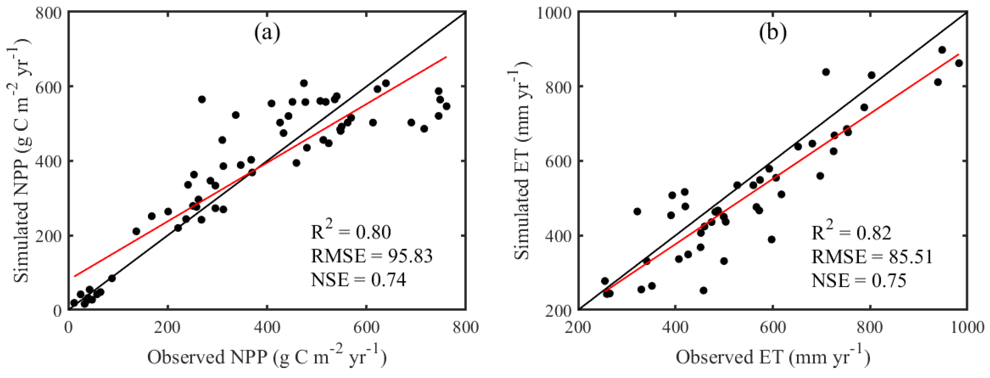
The accuracy of the LPJ model is evaluated by comparing simulated and observed NPP and ET (Figure 2). The simulated NPP closely matched the observations (R2 = 0.80, NSE = 0.74), indicating that the model had a strong capability to reproduce NPP dynamics (Figure 2a). However, an overestimation trend was identified, with an RMSE of 95.83 gC·m−2, suggesting discrepancies at certain sites. The consistency between simulated and observed ET was also high (R2 = 0.82, NSE = 0.75), with a relatively low RMSE of 85.51 mm, reflecting a modest overall error (Figure 2b). Nevertheless, ET was still underestimated, particularly in regions with high evapotranspiration. Overall, the LPJ model performed well in simulating the vegetation carbon–water cycle on the TP, providing a reliable basis for subsequent scenario projections and process-based analyses.
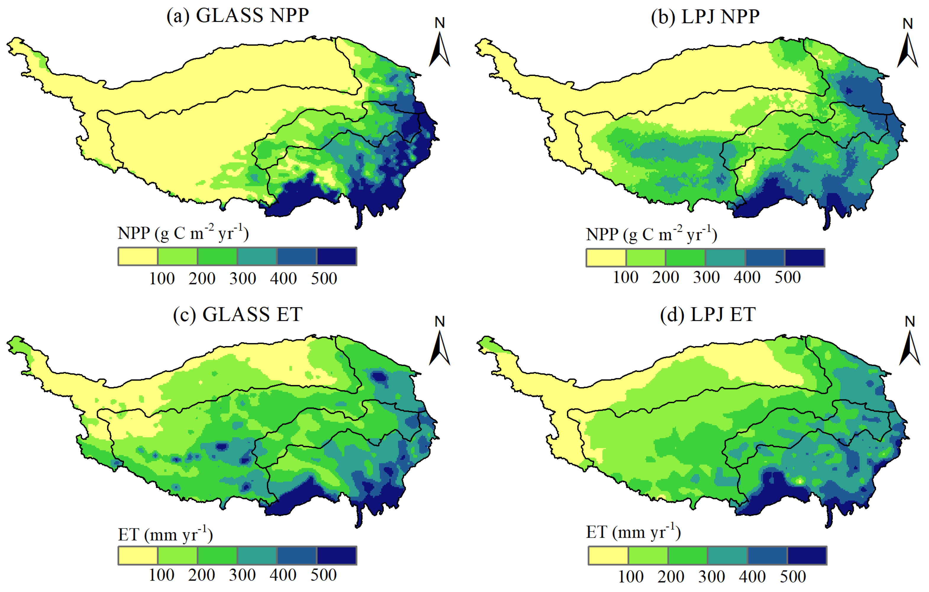
Figure 3 is presented to illustrate the mean annual spatial patterns of NPP and ET across the TP during 1982–2018 based on satellite observations and LPJ model simulations. Both datasets exhibited a distinct northwest–southeast increasing gradient in NPP and ET. NPP and ET remained low in the arid northwestern region but reached substantially higher levels in the southeastern region, where the monsoon influence is strong and vegetation growth conditions are generally more favorable. The comparison between observations and simulations showed that the mean annual NPP during the study period was 169.68 and 188.92 g C m−2 yr−1, respectively (Figure 3a,b). Observed and simulated mean annual ET were 235.75 and 222.31 mm yr−1, respectively (Figure 3c,d). Overall, the LPJ model reproduced the principal spatial patterns of NPP and ET across the TP with reasonable accuracy and provided a robust basis for assessing vegetation–water yield interactions under climate change.
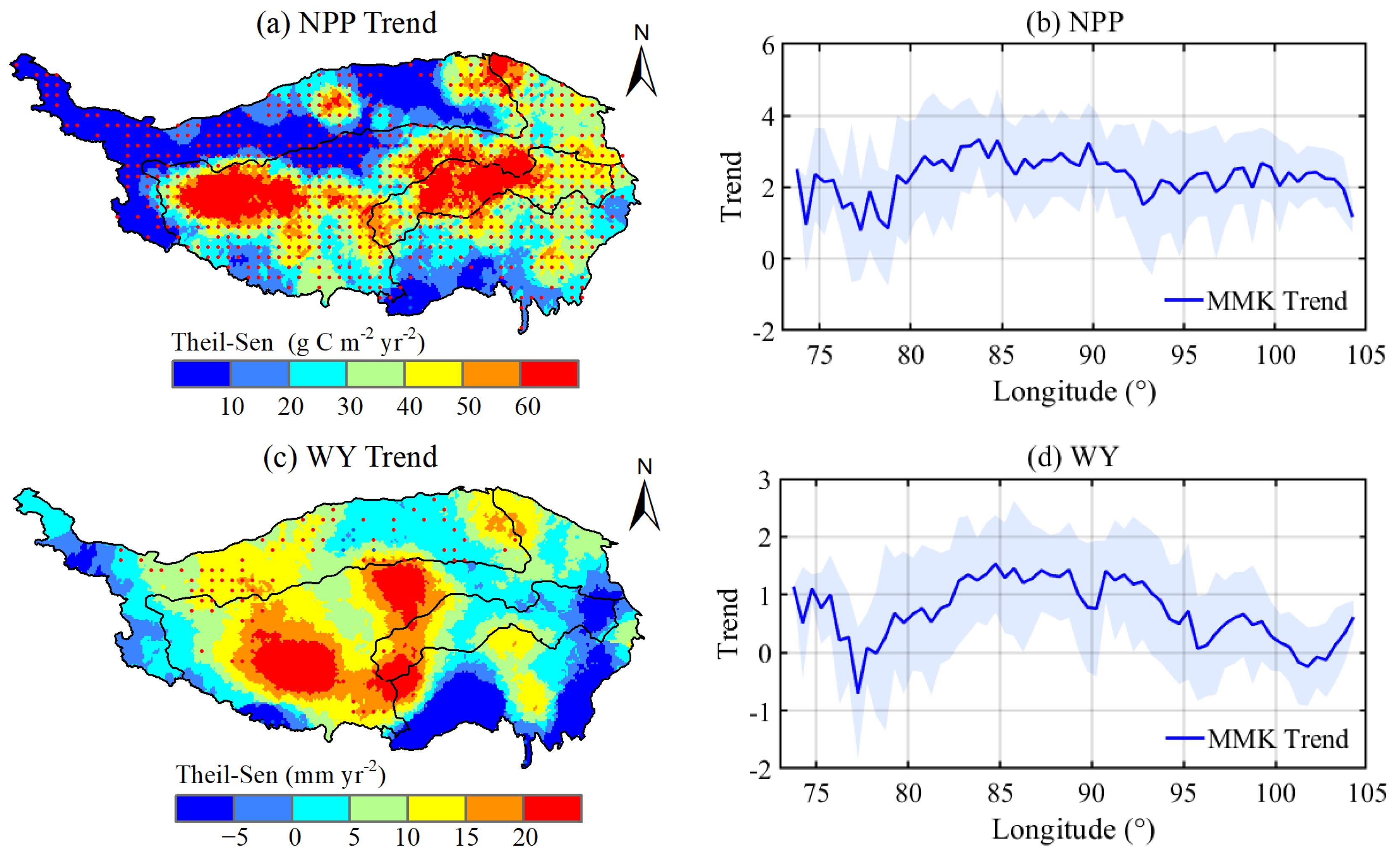
Figure 4 illustrates long-term spatial trends in NPP and WY across the TP during 1981–2020. According to Figure 4a, an increasing NPP trend was detected over 89.51% of the study area, most evident in the central and eastern Plateau, indicating a sustained improvement in vegetation productivity during recent decades. The longitudinal variation curve showed that NPP increased markedly between 80° E and 90° E, while the shaded area represented standard deviations, reflecting spatial fluctuations among different regions (Figure 4b). For WY, Figure 4c shows that 77.39% of the TP experienced positive trends, with notable increases concentrated in the central region. Areas exhibiting declining WY covered 22.61% of the total area and were primarily located in humid zones. Along the longitudinal direction, WY exhibited a similar overall pattern to NPP, with a distinct increase between 80° E and 90° E (Figure 4d). These results suggested that vegetation productivity and water yield exhibited a certain degree of spatiotemporal coupling across the TP.
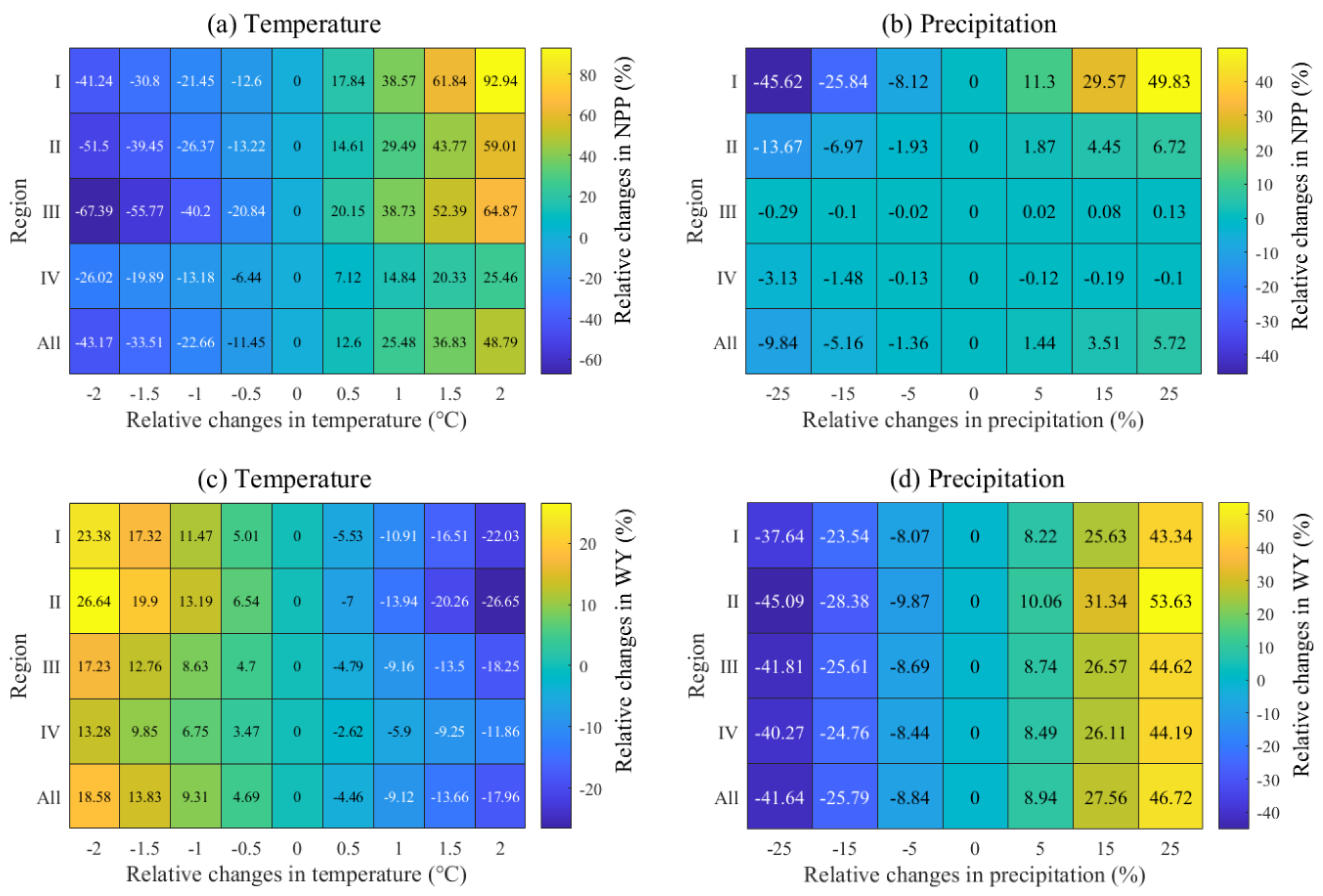
Sensitivity of the LPJ model was assessed by varying its input parameters (Figure 5). The values shown indicate the relative change rates of NPP and WY with respect to the historical baseline period. NPP responses to temperature changes exhibited pronounced spatial heterogeneity (Figure 5a). The I and II regions exhibited the highest sensitivity, with NPP increasing by 92.94% and 59.01%, respectively, under a 2 °C warming scenario. These results indicated that temperature increases substantially enhanced vegetation productivity in water-limited regions. Conversely, NPP in the humid region responded less strongly, indicating that temperature was less influential where water was abundant. Across most regions, precipitation changes exerted a relatively weak influence on NPP (Figure 5b). A clear response was detected only in the arid region, where a 25% increase in precipitation led to a 49.83% rise in NPP. Other zones exhibited negligible sensitivity, indicating that in more humid regions, NPP was not strongly constrained by precipitation.
WY responded negatively to temperature increases across all regions, particularly in the I and II regions (Figure 5c), reflecting enhanced evapotranspiration and reduced water availability under warming conditions. In contrast, WY responded strongly and positively to increased precipitation across the Plateau (Figure 5d). A 25% increase in precipitation resulted in a 46.72% increase in WY at the regional scale, with the largest responses occurring in the II and IV regions. Overall, NPP in the TP was found to be more sensitive to temperature increases, whereas WY was primarily driven by changes in precipitation. The findings emphasized that climate change affected both vegetation productivity and water availability, with warming promoting carbon sequestration while intensifying water deficits in vulnerable areas.

3.2. Quantifying the Contributions of WY and Climatic Factors to Variations in Vegetation NPP

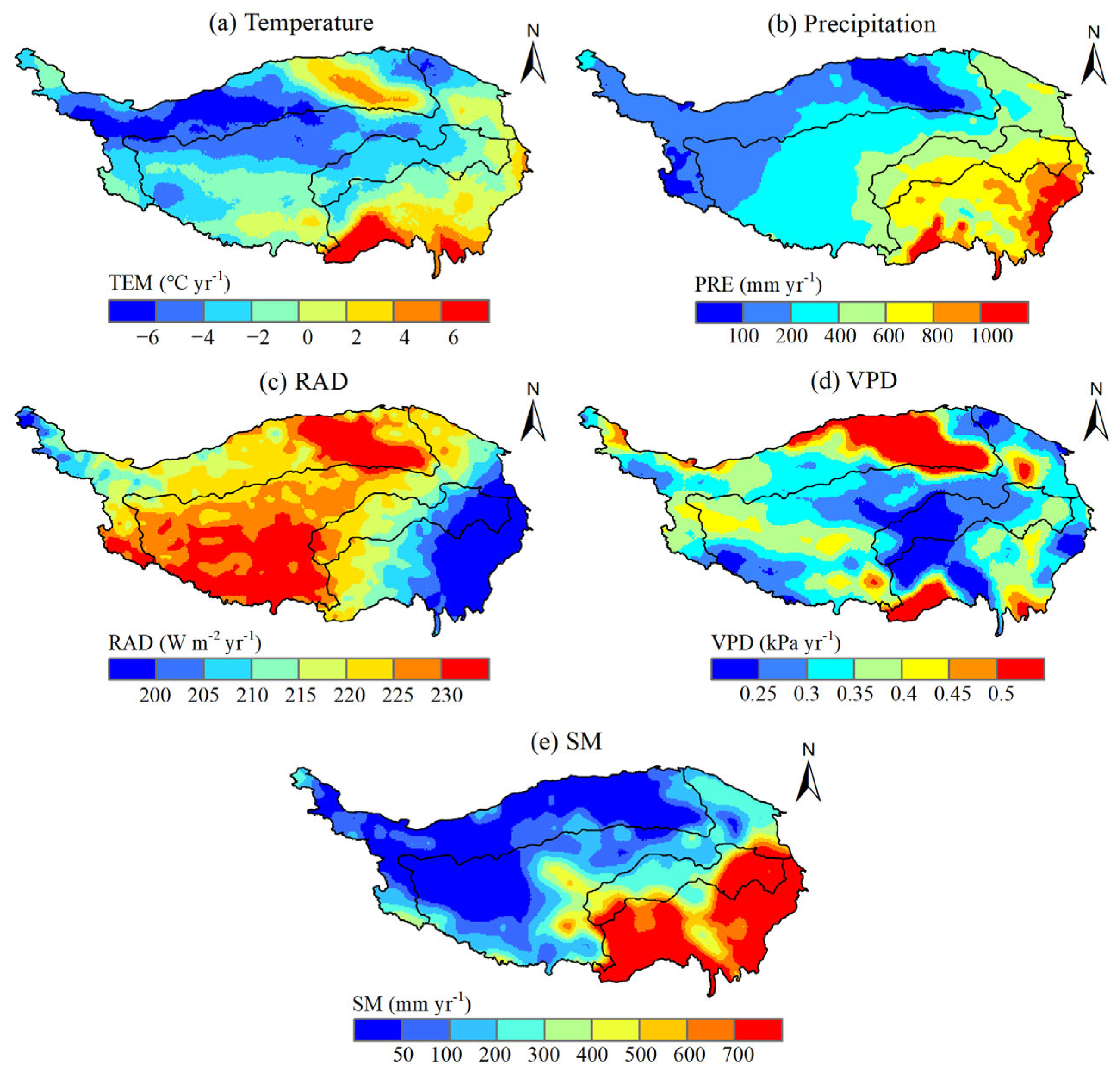
The spatial pattern of vegetation-driving factors across the TP during 1981–2020 is displayed in Figure 6. Mean annual TEM exhibited a general southeast–northwest decline (Figure 6a). Mean annual PRE also showed a southeast–northwest decreasing pattern, with values in the southeast exceeding 1000 mm, whereas precipitation in the northwest was less than 100 mm (Figure 6b). The western and southern regions generally received more than 220 W m−2 of radiation annually, while the southeastern region had lower radiation levels, below 200 W m−2 (Figure 6c). Elevated VPD levels were observed in the northern and western parts of the Plateau, generally exceeding 0.5 kPa, whereas comparatively low VPD conditions (<0.25 kPa) prevailed across the central and southeastern regions (Figure 6d). SM also showed a distinct spatial gradient, with the southeastern region having relatively high soil water content, reaching up to 700 mm, while the northwestern and southwestern areas were drier, with values below 50 mm (Figure 6e).
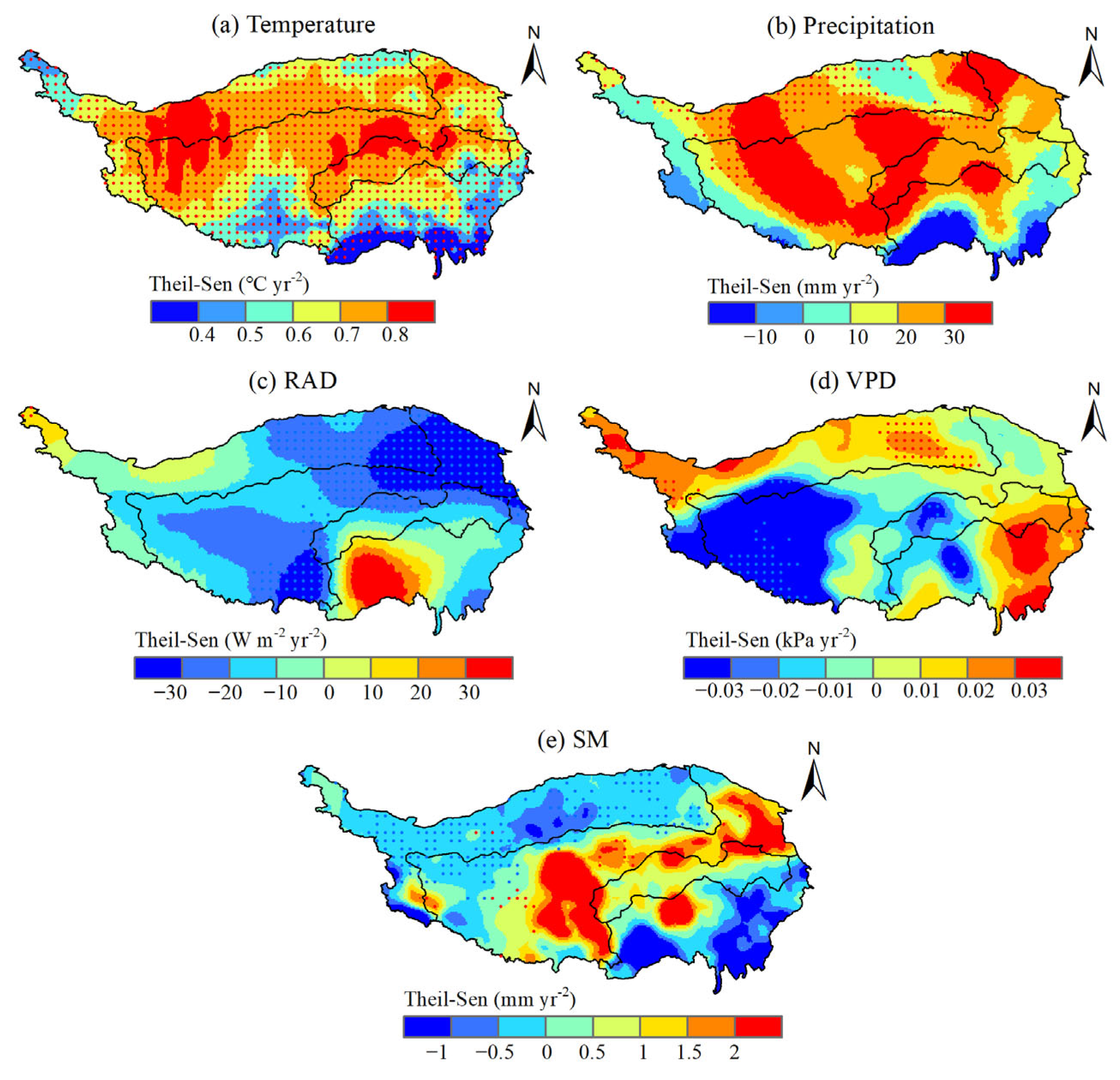
Spatial variations in the principal climatic drivers across the TP from 1981 to 2020 are presented in Figure 7. Overall, temperature exhibited a significant increasing trend, with particularly strong warming observed across the central, eastern, and northern TP, where the Theil–Sen slopes generally exceeded 0.6 °C yr−2, indicating a pronounced regional warming pattern (Figure 7a). Precipitation showed substantial spatial heterogeneity, characterized by notable increases in the northwestern and central regions and slight decreases in the southeast, reflecting an overall tendency toward wetter conditions (Figure 7b). RAD generally decreased, especially in the northern and western TP, suggesting a weakening of radiative energy input over the region (Figure 7c).
The VPD displayed a distinct east–west gradient, with higher values in the eastern TP indicating intensified atmospheric dryness, whereas the southwestern and central regions experienced a slight decline (Figure 7d). SM increased markedly in the central TP but declined in the northern and southern parts, revealing a spatially divergent pattern of wetting and drying under the ongoing warming trend (Figure 7e). Overall, the TP underwent a compound climate signal characterized by warming, wetting, reduced solar radiation, and pronounced hydroclimatic divergence over the past four decades. These climatic variations collectively shaped the spatiotemporal dynamics of NPP across the region.
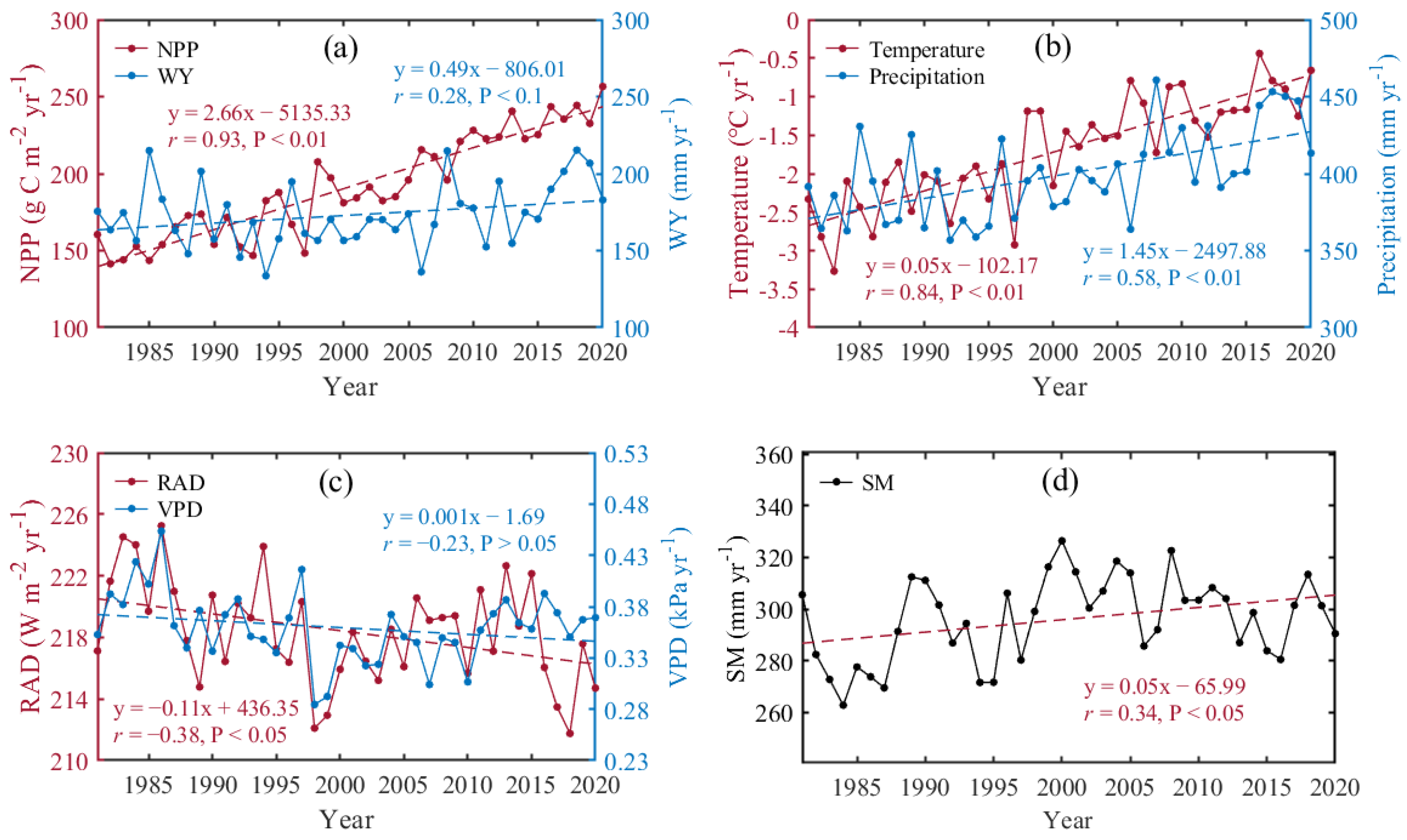
Temporal changes in annual mean NPP and its associated climatic drivers across the TP from 1981 to 2020 are presented in Figure 8. Over this period, NPP increased significantly by 2.66 g C m−2 yr−1 (Figure 8a). WY also exhibited an increasing trend, although the magnitude was comparatively smaller. Temperature increased significantly by 0.05 °C yr−1, accompanied by a concurrent rise in precipitation of 1.45 mm yr−1 (Figure 8b). In contrast, RAD showed a significant declining trend, whereas variations in VPD were not statistically significant (Figure 8c). Soil moisture increased overall (0.05 mm yr−1) with notable interannual variability and showed a significant correlation with NPP (Figure 8d). Collectively, these results suggest that rising temperatures together with enhanced moisture availability have promoted vegetation productivity across the TP.
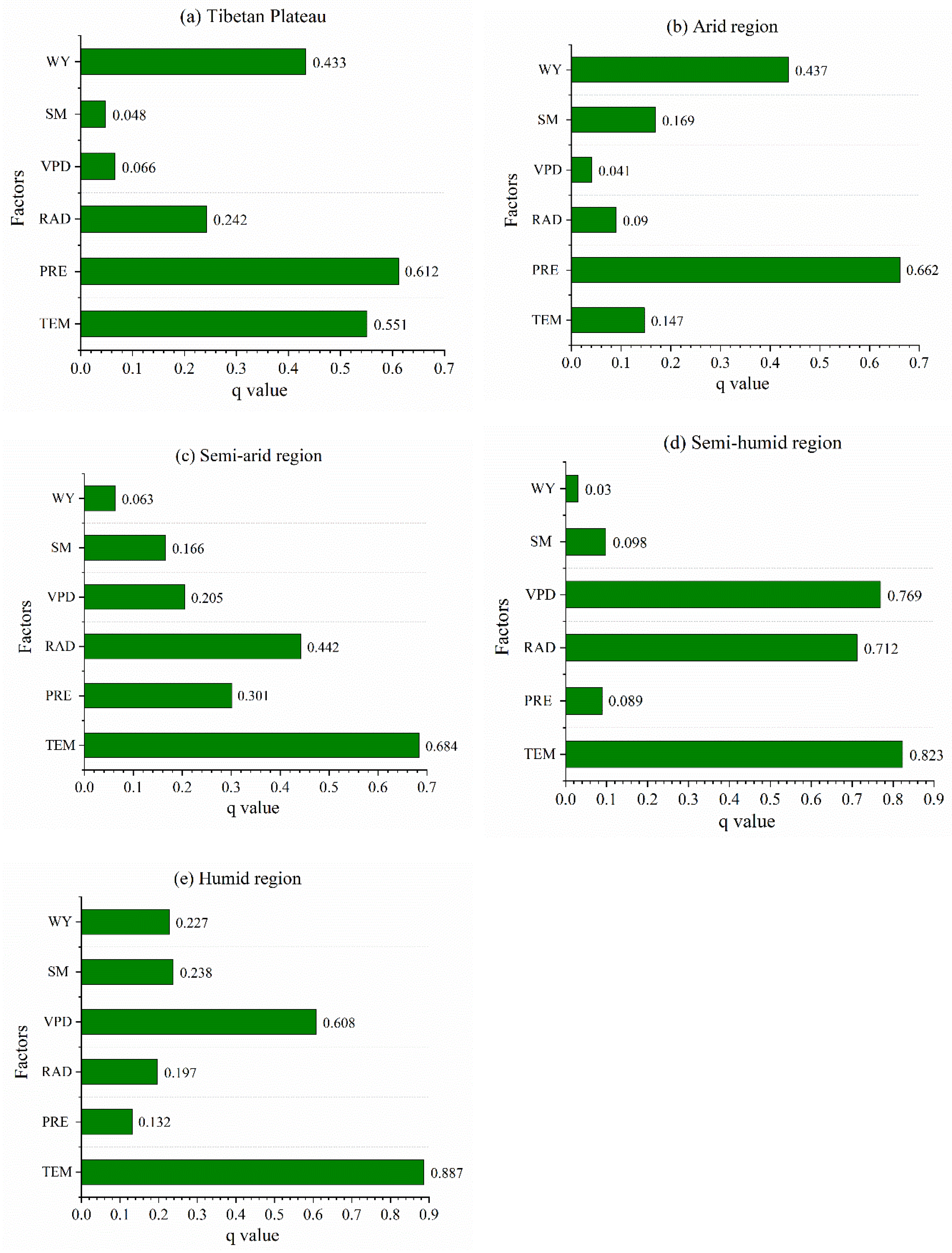
Geodetector analysis revealed a pronounced spatial heterogeneity in vegetation responses to environmental drivers. Figure 9a shows that PRE exhibited the strongest association with vegetation NPP across the TP (q = 0.612), followed by TEM (q = 0.551) and WY (q = 0.433), highlighting the importance of both moisture and temperature related factors. In the arid region, PRE exhibited the highest explanatory power (q = 0.662), significantly exceeding that of other variables, suggesting that the spatial variability of vegetation NPP in these areas was strongly associated with precipitation availability (Figure 9b). WY ranked second (q = 0.437), while factors such as VPD and RAD played relatively minor roles. According to Figure 9c, TEM emerged as the dominant driver, followed by RAD and PRE in the semi-arid region. This pattern indicated that spatial variations in NPP were more closely associated with thermal and radiative conditions in this transitional zone.
In the semi-humid region, TEM, VPD, and RAD were the principal contributors to vegetation NPP, highlighting strong spatial linkages between NPP and thermal conditions as well as atmospheric evaporative demand (Figure 9d). In the humid region, TEM was the dominant driver (q = 0.887), followed by VPD (q = 0.608; Figure 9e). As water availability was generally less limiting in the humid region, the spatial distribution of NPP was more strongly associated with thermal energy and atmospheric moisture conditions. Overall, the dominant environmental factors associated with vegetation NPP varied markedly among subregions. Precipitation showed the strongest spatial association with NPP in the arid region, whereas temperature and VPD exhibit higher explanatory power in the humid region, reflecting contrasting climatic constraints across moisture gradients.
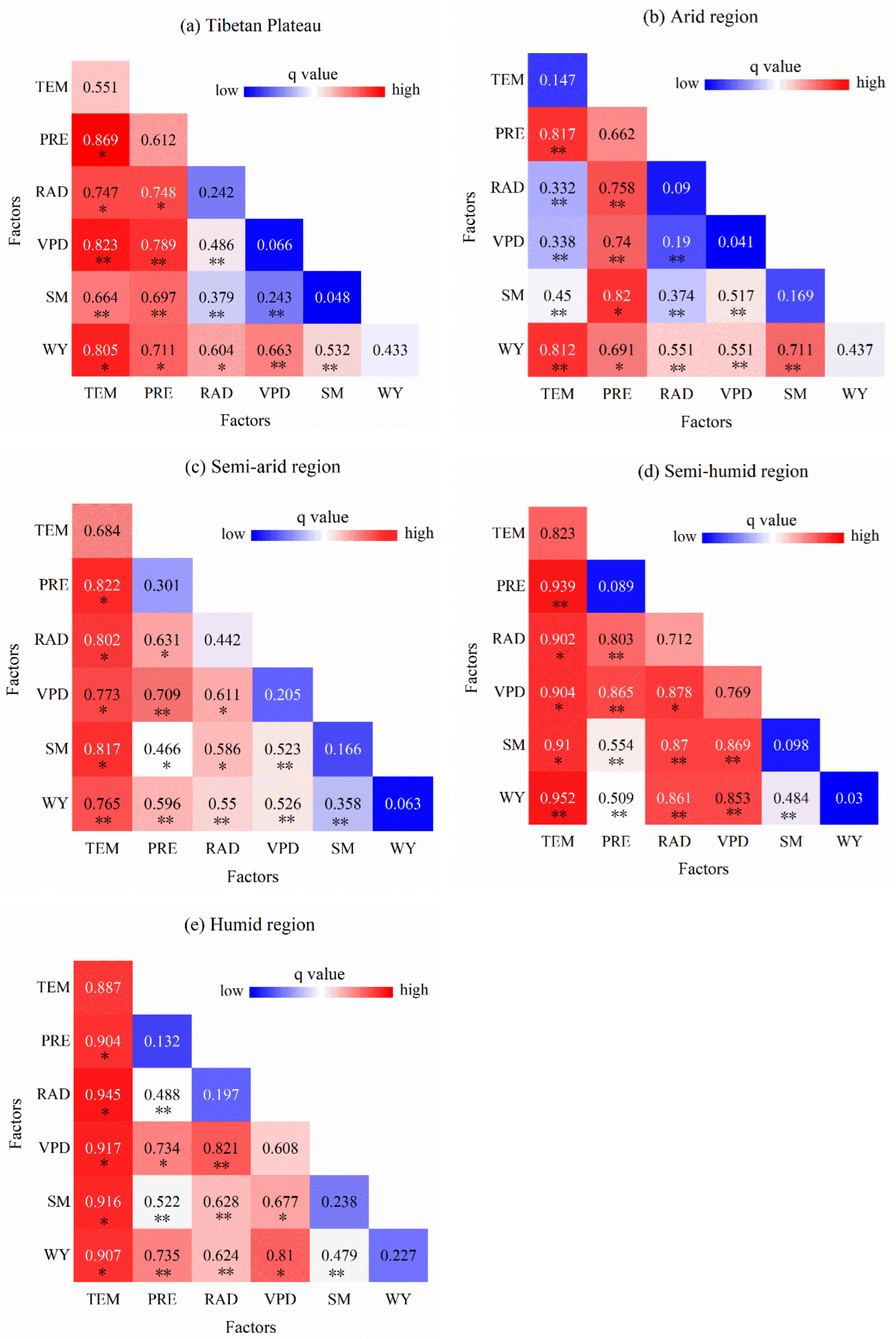
Figure 10 illustrates the interactions between ecological and environmental factors influencing vegetation NPP across the TP and its subregions. On the TP, the most prominent interactions were observed between PRE and TEM (q = 0.869), and between PRE and WY (q = 0.805), suggesting that the combined effects of moisture- and temperature-related variables substantially enhanced the explanation of NPP spatial patterns (Figure 10a). In the arid region, the strongest interactions were observed between WY × PRE and PRE × TEM, highlighting strong spatial synergies among water-related variables in explaining NPP variability under moisture-limited conditions (Figure 10b).
In the semi-arid region, the dominant interactions included PRE×TEM and VPD × RAD, indicating that the spatial distribution of vegetation NPP was closely associated with the combined effects of precipitation, thermal conditions, and atmospheric evaporative demand (Figure 10c). In the semi-humid region, the strongest interactions were observed for PRE × TEM (q = 0.939) and RAD × TEM (q = 0.902), both demonstrating nonlinear enhancement, suggesting that multi-factor interactions involving TEM, RAD, and PRE provide substantially higher explanatory power for NPP spatial variability than individual factors alone (Figure 10d). In the humid region, nearly all major factors exhibited strong interactions, indicating that under conditions of relatively sufficient water availability, the spatial variability of NPP was more strongly associated with nonlinear synergies among energy-related variables and atmospheric moisture indicators (Figure 10e).

3.3. Future Responses of WY to Vegetation Dynamics and Climate Change

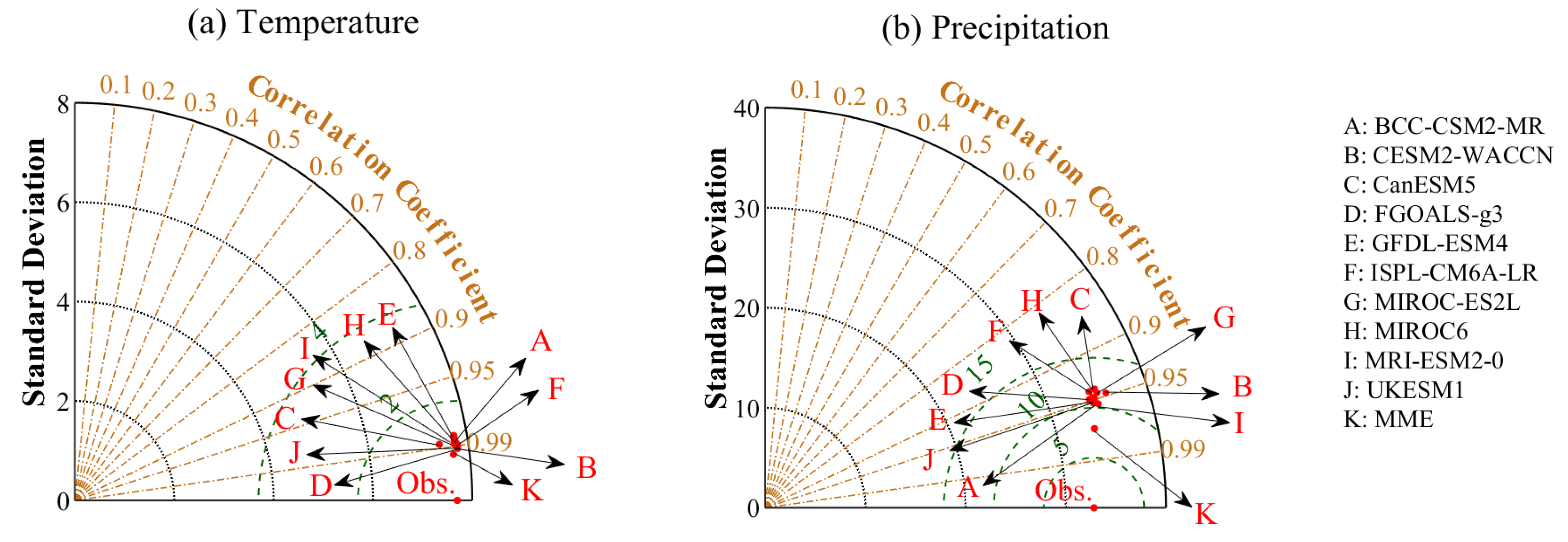
Taylor diagrams were used to assess the performance of CMIP6 models by comparing simulated and observed temperature and precipitation across the TP for 1981–2014 (Figure 11). Climate model performance was assessed using standard deviation (SD), correlation coefficient, and centered root-mean-square error (RMSE). For temperature simulations, most models exhibited strong agreement with observations, with correlation coefficients exceeding 0.98, indicating that these models effectively captured the temporal variability of temperature (Figure 11a). In addition, the centered RMSE values for all models were below 1.31, suggesting high accuracy in reproducing temperature fluctuations.
For precipitation, the correlation coefficients between model outputs and observations were all above 0.94, though overall consistency was lower compared to temperature simulations (Figure 11b). The RMSE values for precipitation were generally above 7.92, indicating larger deviations in simulated precipitation variability. Nevertheless, the MME performed better than individual models, demonstrating a stronger capability in capturing the spatiotemporal patterns of precipitation. Taken together, the CMIP6 multi-model ensemble showed better overall performance in simulating temperature than precipitation. The MME exhibited the best performance for both variables, confirming the effectiveness of ensemble modeling in improving the reliability of regional climate simulations across the TP.
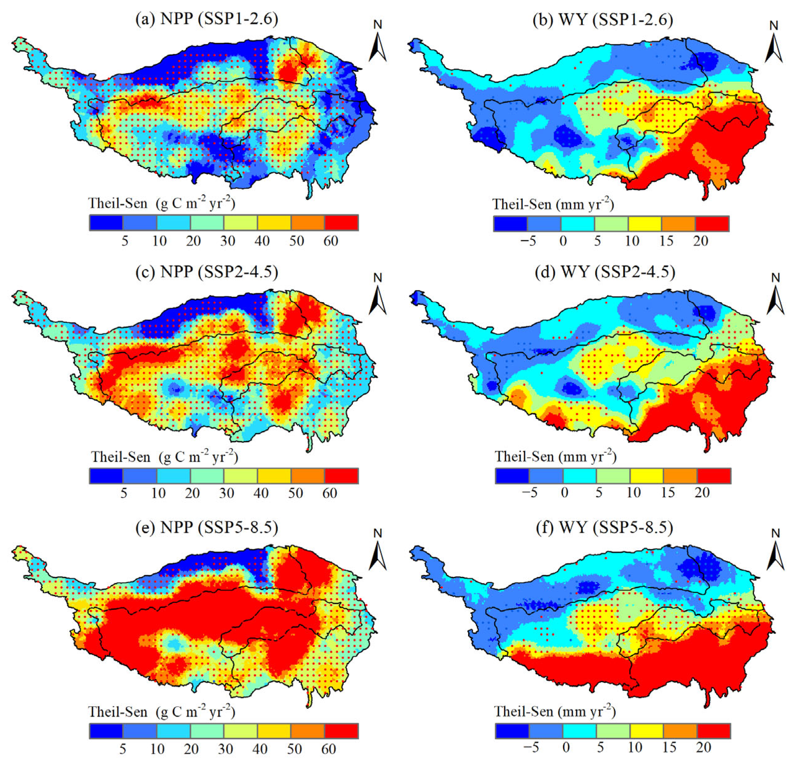
Spatial variations in NPP and WY change rates across the TP during 2015–2060 are illustrated in Figure 12. Under three SSP scenarios, the proportion of the area showing a rising trend in NPP was 86.15%, 90.94%, and 95.62%, respectively, with significantly increasing areas accounting for 68.73%, 80.65%, and 84.52% (Figure 12a,c,e). Across most regions, NPP increased, exceeding 30 g C m−2 yr−2, with some areas exceeding 60 g C m−2 yr−2, suggesting that climate change positively influenced vegetation carbon sequestration. Additionally, under the three SSP scenarios, 69.24%, 72.81%, and 73.01% of the area exhibited upward trends in WY, with significantly increasing regions comprising 31.57%, 30.35%, and 42.67%, respectively (Figure 12b,d,f). The southeastern TP showed a marked increase in WY (>20 mm yr−1), whereas the northwestern TP generally exhibited a declining trend. These results suggested that although NPP increased widely over the region, the uneven distribution of water resources and the intensifying water scarcity in the arid region could pose sustainability challenges. Overall, with the increase in emission scenario severity, the vegetation carbon sink capacity of the TP was significantly enhanced, but the sustainability of water resources in the arid region faced increasing pressure.
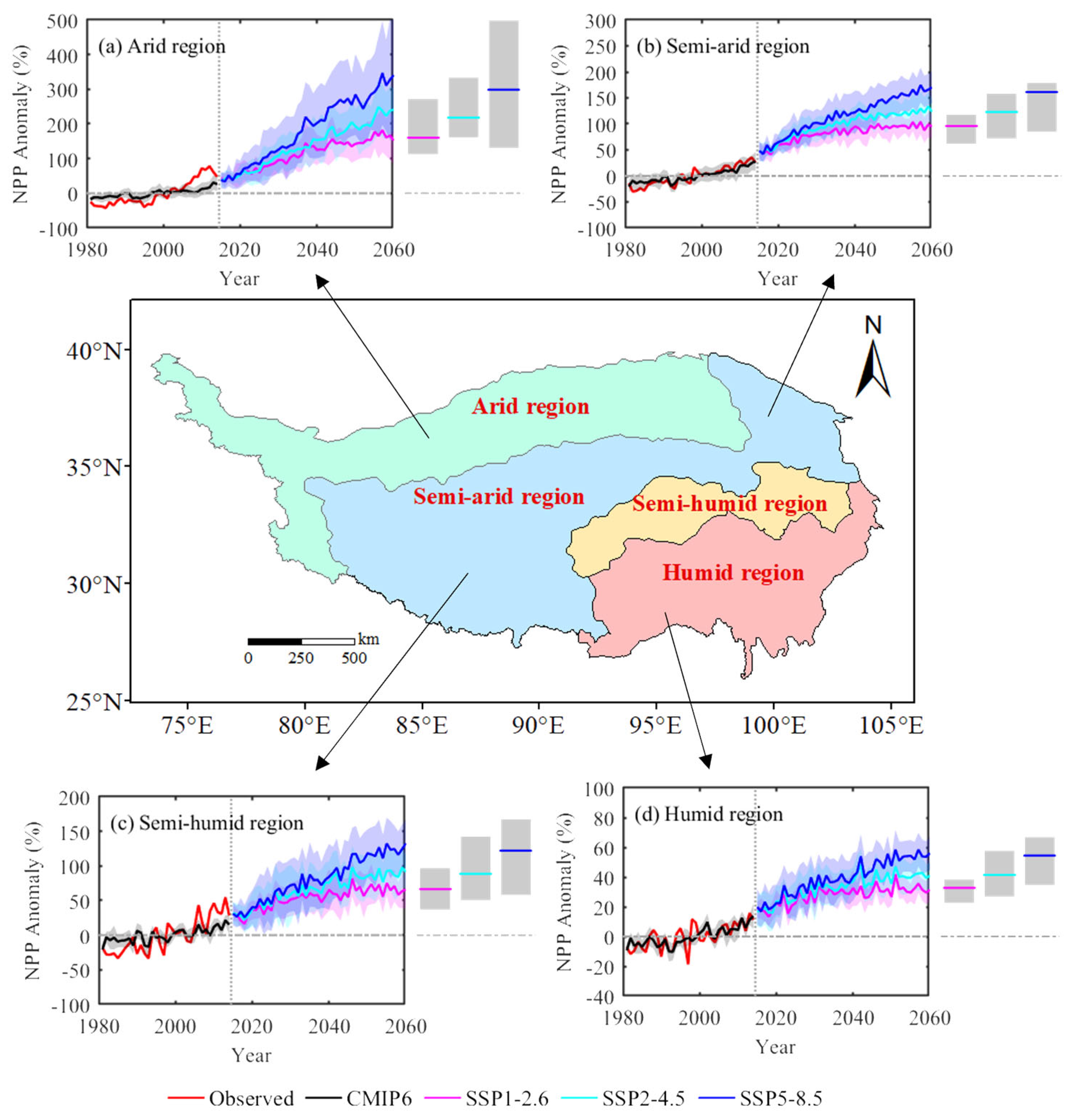
Figure 13 illustrates the range of uncertainties in vegetation NPP anomalies across the TP from 1981 to 2060 under three SSP scenarios, relative to the historical period of 1981–2014. NPP anomalies in all four subregions exhibited an increasing trend over time, with greater increases observed under higher emission scenarios. Nevertheless, different regions showed markedly varied responses to climate change. The arid region showed the most pronounced increase in NPP, where under the SSP2-4.5 and SSP5-8.5 scenarios, the NPP anomaly exceeded 200% (Figure 13a). In comparison, the semi-arid region also experienced a significant increase in NPP anomalies, but the magnitude of change was slightly lower than that of the arid region (Figure 13b). In the semi-humid region, by 2060, NPP anomalies were projected to increase by 65.8%, 91.44%, and 132.54% under the three scenarios (Figure 13c). Similarly, in the humid region, NPP anomalies were projected to increase by 31.46%, 40.76%, and 56.04% by 2060 under the respective scenarios (Figure 13d). On the whole, NPP responses to future climate change exhibited significant spatial heterogeneity across different hydroclimatic zones of the TP. Although the arid and semi-arid regions demonstrated high carbon sequestration potential, they also exhibited lower ecosystem stability. In contrast, the humid region remained relatively stable and played an important role in maintaining the regional carbon balance.
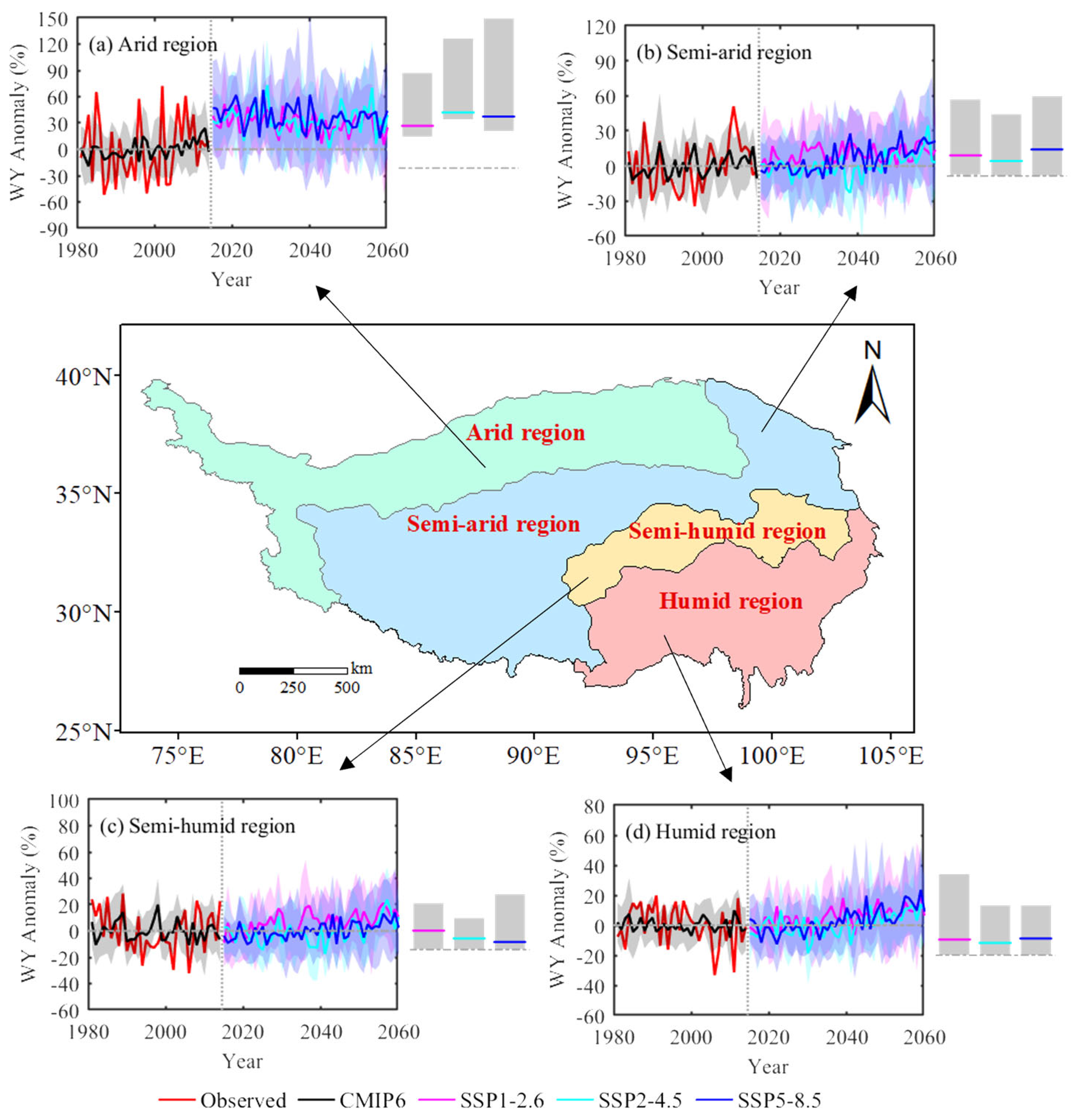
Figure 14 illustrates the temporal evolution of WY anomalies across four climatic subregions of the TP from 1981 to 2060 under three SSP scenarios. Overall, the projected variations in WY anomalies exhibited distinct regional disparities. In the arid region, WY anomalies generally showed a decreasing trend with a fluctuation range of approximately ±50%, accompanied by pronounced interannual variability (Figure 14a). This indicated that the arid region was more sensitive to climatic perturbations and exhibited greater hydrological uncertainty and ecological vulnerability. In the semi-arid region (Figure 14b), WY anomalies fluctuated within a similar range (±30%) but displayed a slight increasing trend across the SSP scenarios. In contrast, the semi-humid and humid regions (Figure 14c,d) experienced relatively minor changes, with WY anomalies remaining within ±20% throughout the study period. These regions exhibited more stable hydrological responses, suggesting stronger system resilience to future climate change compared with the arid and semi-arid regions. Overall, under future climate change scenarios, WY in the arid and semi-arid regions of the TP showed considerable variability and uncertainty, whereas the semi-humid and humid regions maintained relatively stable hydrological conditions, reflecting distinct spatial heterogeneity in the regional water-yield responses to climate change.

4. Discussion

4.1. Spatiotemporal Variations of NPP and WY Across the TP

This study revealed that from 1981 to 2020, the TP experienced a pronounced warming and wetting trend, with temperature and precipitation showing annual increases of 0.05 °C and 1.45 mm, respectively. Similarly, Yu et al. [5] reported pronounced warming accompanied by increased precipitation across the TP over 1961–2020, with temperature and precipitation rising by 0.34 °C and 0.73% per decade, respectively. Notably, this warming–wetting trend has generally favored vegetation growth and promoted ecosystem recovery in the region [4,55]. Zhong et al. [56] demonstrated that the TP experienced a warming trend during the period 1960–2014, and vegetation density showed an overall increasing trend in response to this warming. Luo et al. [57] indicated that the northeastern TP experienced significant warming and humidification from 1982 to 2018, accompanied by notable increases in GPP and ET in the region.
A pronounced southeast-to-northwest gradient in NPP and WY across the TP during 1981–2020 was documented in this study. Furthermore, upward trends occurred in 89.51% and 77.39% of the TP area, respectively, reflecting concurrent improvements in vegetation productivity and water availability. These results align with earlier research. Sun et al. [37] showed that NPP over the TP increased markedly during 2000–2020 at 0.88 g C m−2 yr−2, with a clear increase from northwest to southeast. Similarly, Jia et al. [58] observed increasing NPP and WY in the TP from 2000 to 2018, following a southeast–northwest gradient. Cui et al. [12] suggested that during the period from 2001 to 2018, changes in vegetation increased the availability of global water resources at 0.26 mm yr−2. It is noteworthy that although vegetation greening tends to enhance ET, which negatively impacts WY, this effect is partially offset by the positive feedback of increased precipitation, thereby alleviating the pressure on regional water resources caused by increased ET [59].

4.2. Dominant Climatic and Hydrological Controls on Vegetation NPP

Vegetation development was strongly affected by temperature and precipitation [33]. Sensitivity analysis showed that NPP increased with rising temperatures and increasing precipitation. In addition, WY was more sensitive to precipitation changes and exhibited a negative correlation with temperature. Lin et al. [60] reported that TP grassland NPP during 1901–2010 increased in association with rising temperature, precipitation, and atmospheric CO2. Zhong et al. [56] revealed that vegetation types exhibited varying responses to climate change, with grasslands in the TP’s semi-arid region particularly sensitive to temperature and precipitation fluctuations. Cuo et al. [61] based on LPJ model simulations, also confirmed that NPP was significantly correlated with temperature, precipitation, and cloud cover, with a one-month lag effect.
In addition, other factors such as VPD, RAD, and SM also showed significant associations with NPP dynamics. Results from the Geodetector analysis indicated that precipitation, temperature, and WY jointly exhibited relatively high explanatory power for the spatial variability of NPP over the TP. Similar patterns have also been reported in previous studies. Piao et al. [62] demonstrated that precipitation contributed most strongly to grassland NPP increases on the TP, followed by rising atmospheric CO2 concentrations and temperature. Similarly, Liu et al. [63] found that precipitation, temperature, and CO2 collectively served as the major contributors to the observed increase in vegetation cover across the TP. However, the dominant controlling factors associated with vegetation NPP varied markedly across the different ecological regions of the TP. In the arid region, precipitation and WY exhibited stronger associations with vegetation NPP, suggesting that water availability plays a dominant limiting role under moisture-constrained conditions. Consistent with this pattern, previous studies have identified water availability as the key constraint on vegetation restoration in arid areas [13,64]. In arid and semi-arid regions, NPP was more closely associated with temperature, RAD, and precipitation, reflecting the combined effects of low temperature, limited rainfall, and high elevation on photosynthesis. Thus, adequate precipitation, optimal temperatures, and high photosynthetically active radiation favor plant growth [65]. Conversely, NPP in humid and semi-humid regions showed stronger associations with temperature, VPD, and RAD. In these water-abundant areas, extended sunshine is generally considered critical for prolonging photosynthesis, thereby promoting vegetation growth [66].

4.3. Implications of Vegetation Dynamics and Climate Change for Future WY

This study highlights the pivotal role of WY in shaping vegetation NPP across the entire TP, identifying WY as a key determinant of vegetation dynamics. Moreover, the vegetation response to WY was projected to become increasingly pronounced under future climate scenarios. Under the three SSP scenarios, areas with increasing NPP account for 86.15%, 90.94%, and 95.62%, respectively. Meanwhile, the proportion of the area with increasing WY was 69.24%, 72.81%, and 73.01%, respectively. Similarly, Gao et al. [67] projected that NPP across the TP would increase by 79% and 134% under the RCP4.5 and RCP8.5 scenarios, respectively. Zhang et al. [8] based on CMIP6 projections, reported a sustained increase in LAI across northern China and the TP throughout the 21st century, with most areas experiencing simultaneous increases in both LAI and WY. Yan et al. [2] demonstrated that under future SSP scenarios, the trade-off between a warming-wetting climate and vegetation dynamics could enhance regional hydrological resilience. However, as the vegetation carbon sink increased substantially, its associated impacts on the arid regions of the TP intensified. Relative to the baseline period, the magnitude of changes in NPP and WY during 2021–2060 varied across different ecological regions. The arid region showed the largest increase in vegetation NPP, reflecting their higher sensitivity to climate change. Likewise, interannual variability of WY was more pronounced in arid areas, indicating greater uncertainty and ecological vulnerability in these regions.

4.4. Limitations and Prospects

This study involves several sources of uncertainty. First, satellite-based products are susceptible to atmospheric conditions, solar angles, and other external factors, which may bias data accuracy [68]. In addition, the lack of extensive ground-based observations across the TP limits the possibility of comprehensive ground-truthing. Second, the LPJ model does not account for all dynamic ecosystem processes, such as nitrogen deposition and nutrient limitations, which may bias simulations of ecosystem responses under certain environmental conditions [45]. Furthermore, despite the LPJ model’s widespread use in assessing ecosystem responses to future climate change, the climate projections inherently contain uncertainties [67]. Third, an important limitation of this study is the absence of an explicit representation of groundwater processes. Recent studies suggest that groundwater storage and exchange may contribute substantially to the overall water budget of the TP, potentially reaching up to approximately 85% of total water resources [69]. In the present study, WY is estimated based on the difference between precipitation and ET, implicitly assuming that long-term changes in subsurface water storage are negligible. This assumption may not fully capture the role of groundwater–surface water interactions, particularly in regions where groundwater recharge, discharge, or lateral flow plays a dominant role. As a result, the estimated WY may represent an effective surface water balance rather than the complete terrestrial water budget.
Despite these limitations, the model provides insight into the coupled NPP–WY responses to climate change and greening at regional scales. Future research should prioritize the explicit integration of groundwater dynamics into vegetation–hydrology modeling frameworks, including the coupling of dynamic global vegetation models with groundwater or land surface models. Such advances would facilitate a more comprehensive assessment of vegetation–water interactions and improve our ability to quantify ecosystem–hydrological feedback in the context of climate change.

5. Conclusions

This study employed the LPJ model driven by CMIP6 data to investigate the responses of vegetation NPP to WY across different ecological zones of the TP from the historical period (1981–2020) to the future (2021–2060), and applied the Geodetector method to identify the main drivers of NPP variability. The major findings were as follows:
(1) Over the past four decades, most areas of the TP showed increasing trends in both vegetation NPP and WY. Sensitivity analyses indicated that a 2 °C warming increased NPP by 48.79% but reduced WY by 17.96%. In contrast, a 25% increase in precipitation led to only a modest rise in NPP (5.72%) but substantially enhanced WY (46.72%). These results suggested that warming strongly stimulated vegetation growth while intensifying water consumption, whereas increased precipitation improved water availability but contributed little to additional vegetation gains.
(2) Geodetector results revealed that precipitation, temperature, and WY jointly shaped the spatial pattern of NPP across the TP, with q-values of 0.612, 0.551, and 0.433, respectively. The arid region was most strongly constrained by water limitation; the semi-arid region was influenced by both water and energy constraints; and humid to sub-humid regions were primarily regulated by temperature, VPD, and RAD. Moreover, interaction analysis indicated that the combined effects of these factors provided higher explanatory power for NPP variability than individual drivers alone.
(3) Under the SSP1-2.6 scenario, increases in NPP and WY were mainly concentrated in the central and southeastern TP. Under the SSP2-4.5 and SSP5-8.5 scenarios, NPP increases became substantially stronger, while WY exhibited pronounced spatial heterogeneity and a clear dry–wet divergence. Compared with the historical period, the pattern of vegetation impacts on hydrological processes shifted, with water availability increasing in the humid regions but declining in the arid regions. These findings suggest that in climatically vulnerable areas, rapid vegetation growth may intensify water consumption, thereby heightening ecosystem fragility and hydrological risks.

Author Contributions

R.K.: data curation, formal analysis, methodology, writing—original preparation. Z.Z.: writing—review and editing. J.H.: supervision, writing—review and editing. D.Y.: conceptualization, supervision. W.S.: methodology, software. X.L.: formal analysis, software. H.Z.: investigation, methodology. J.T.: formal analysis, methodology. All authors have read and agreed to the published version of the manuscript.

Funding

This study was supported by the Nanxun Scholars Program for Young Scholars of ZJWEU (Grant No. RC2024021419); the Open Research Fund of State Key Laboratory of Water Cycle and Water Security (Grant No. SKL-WAWS-KFMS202502); and the Zhejiang Provincial Natural Science Foundation of China (Grant No. LTGS24D010001).

Data Availability Statement

Data will be made available on request.

Conflicts of Interest

The authors declare no conflicts of interest.

Abbreviations

WYWater yield
NPPNet primary productivity
GPPGross primary productivity
ETEvapotranspiration
LAILeaf area index
PREPrecipitation
TEMTemperature
RADSolar radiation
VPDVapor pressure deficit
SMSoil moisture
LPJLund–Potsdam–Jena
DGVMDynamic Global Vegetation Model
BIOMEBiogeography, Biogeochemical Cycles
GCMGlobal climate model
SSPsShared Socioeconomic Pathways
RCPsRepresentative Concentration Pathways
CMIP6Coupled Model Intercomparison Project Phase 6
MMEMulti-model ensemble
PFTsPlant functional types
MMKModified Mann–Kendall
TPTibetan Plateau

References

  1. Chen, C.; Park, T.; Wang, X.; Piao, S.; Xu, B.; Chaturvedi, R.K.; Fuchs, R.; Brovkin, V.; Ciais, P.; Fensholt, R.; et al. China and India lead in greening of the world through land-use management. Nat. Sustain. 2019, 2, 122–129. [Google Scholar] [CrossRef] [Scilit]
  2. Yan, Y.; Liua, Z.; Chen, L.; Chen, X.; Lin, K. Earth greening and climate change reshaping the patterns of terrestrial water sinks and sources. Proc. Natl. Acad. Sci. USA 2025, 122, e2410881122. [Google Scholar] [CrossRef] [Scilit] [PubMed]
  3. Dong, L.; Wang, X. Inconsistent influence of temperature, precipitation, and CO2 variations on the plateau alpine vegetation carbon flux. npj Clim. Atmos. Sci. 2025, 8, 91. [Google Scholar] [CrossRef] [Scilit]
  4. Wei, Y.; Lu, H.; Wang, J.; Wang, X.; Sun, J. Dual Influence of Climate Change and Anthropogenic Activities on the Spatiotemporal Vegetation Dynamics Over the Qinghai-Tibetan Plateau From 1981 to 2015. Earths Future 2022, 10, e2021EF002566. [Google Scholar] [CrossRef] [Scilit]
  5. Yu, Y.; You, Q.; Zhang, Y.; Jin, Z.; Kang, S.; Zhai, P. Integrated warm-wet trends over the Tibetan Plateau in recent decades. J. Hydrol. 2024, 639, 131599. [Google Scholar] [CrossRef] [Scilit]
  6. Wang, Y.; Lv, W.; Xue, K.; Wang, S.; Zhang, L.; Hu, R.; Zeng, H.; Xu, X.; Li, Y.; Jiang, L.; et al. Grassland changes and adaptive management on the Qinghai–Tibetan Plateau. Nat. Rev. Earth Environ. 2022, 3, 668–683. [Google Scholar] [CrossRef] [Scilit]
  7. Zhu, Q.; Chen, H.; Peng, C.; Liu, J.; Piao, S.; He, J.-S.; Wang, S.; Zhao, X.; Zhang, J.; Fang, X.; et al. An early warning signal for grassland degradation on the Qinghai-Tibetan Plateau. Nat. Commun. 2023, 14, 6406. [Google Scholar] [CrossRef] [Scilit]
  8. Zhang, C.; Long, D.; Liu, T.; Slater, L.J.; Wang, G.; Zuo, D.; Duan, L.; Cui, Y.; Cui, Y. Grassland Greening and Water Resource Availability May Coexist in a Warming Climate in Northern China and the Tibetan Plateau. Earths Future 2023, 11, e2023EF004037. [Google Scholar] [CrossRef] [Scilit]
  9. Liang, C.; Zhang, M.; Wang, Z.; Xiang, X.; Gong, H.; Wang, K.; Liu, H. The strengthened impact of water availability at interannual and decadal time scales on vegetation GPP. Glob. Change Biol. 2024, 30, e17138. [Google Scholar] [CrossRef] [Scilit]
  10. An, Q.; Liu, L.; Wang, L.; Yang, K.; Cheng, Y.; Liu, J.; Huang, G. Contribution of Moisture Recycling to Water Availability in China. Water Resour. Res. 2025, 61, e2024WR038054. [Google Scholar] [CrossRef] [Scilit]
  11. Jia, Z.; Lin, T.; Guo, X.; Zheng, Y.; Geng, H.; Zhang, J.; Chen, Y.; Liu, W.; Lin, M. Vegetation greening mitigates the positive impacts of climate change on water availability in Northwest China. J. Hydrol. 2024, 644, 132086. [Google Scholar] [CrossRef] [Scilit]
  12. Cui, J.; Lian, X.; Huntingford, C.; Gimeno, L.; Wang, T.; Ding, J.; He, M.; Xu, H.; Chen, A.; Gentine, P.; et al. Global water availability boosted by vegetation-driven changes in atmospheric moisture transport. Nat. Geosci. 2022, 15, 982–988. [Google Scholar] [CrossRef] [Scilit]
  13. Gao, S.; Lü, Y.; Jiang, X. Increased precipitation and vegetation cover synergistically enhanced the availability and effectiveness of water resources in a dryland region. J. Hydrol. 2025, 654, 132812. [Google Scholar] [CrossRef] [Scilit]
  14. Lin, S.; Huang, K.; Sun, X.; Song, C.; Sun, J.; Sun, S.; Wang, G.; Hu, Z.; Zhang, Y. Estimates of net primary productivity and actual evapotranspiration over the Tibetan Plateau from the Community Land Model version 4.5 with four atmospheric forcing datasets. J. Plant Ecol. 2024, 17, rtae052. [Google Scholar] [CrossRef] [Scilit]
  15. Liu, W.; Mo, X.; Liu, S.; Lin, Z.; Lv, C. Attributing the changes of grass growth, water consumed and water use efficiency over the Tibetan Plateau. J. Hydrol. 2021, 598, 126464. [Google Scholar] [CrossRef] [Scilit]
  16. Martínez-García, E.; Nilsson, M.B.; Laudon, H.; Lundmark, T.; Fransson, J.E.S.; Wallerman, J.; Peichl, M. Drought response of the boreal forest carbon sink is driven by understorey–tree composition. Nat. Geosci. 2024, 17, 197–204. [Google Scholar] [CrossRef] [Scilit]
  17. Feng, X.; Fu, B.; Piao, S.; Wang, S.; Ciais, P.; Zeng, Z.; Lü, Y.; Zeng, Y.; Li, Y.; Jiang, X.; et al. Revegetation in China’s Loess Plateau is approaching sustainable water resource limits. Nat. Clim. Chang. 2016, 6, 1019–1022. [Google Scholar] [CrossRef] [Scilit]
  18. Kong, R.; Zhu, B.; Zhang, Z.; Zhang, Y.; Huang, R.; Chen, X.; Xu, C.Y. Dissecting the characteristics and driver factors of potential vegetation water use efficiency in China. Sci. Total Environ. 2024, 953, 176174. [Google Scholar] [CrossRef] [Scilit]
  19. Chen, Z.; Wang, W.; Cescatti, A.; Forzieri, G. Climate-driven vegetation greening further reduces water availability in drylands. Glob. Change Biol. 2022, 29, 1628–1647. [Google Scholar]
  20. Sitch, S.; Smith, B.; Prentice, I.C.; Arneth, A.; Bondeau, A.; Cramer, W. Evaluation of ecosystem dynamics, plant geography and terrestrial carbon cycling in the LPJ dynamic global vegetation model. Glob. Change Biol. 2003, 9, 161–185. [Google Scholar]
  21. Chen, G.; Zhuang, H.; Liu, X. Cell-level coupling of a mechanistic model to cellular automata for improving land simulation. GISci. Remote Sens. 2023, 60, 2166443. [Google Scholar] [CrossRef] [Scilit]
  22. Huang, W.; Wang, P.; He, L.; Liu, B. Improvement of water yield and net primary productivity ecosystem services in the Loess Plateau of China since the “Grain for Green” project. Ecol. Indic. 2023, 154, 110707. [Google Scholar] [CrossRef] [Scilit]
  23. Piao, S.; Wang, X.; Park, T.; Chen, C.; Lian, X.; He, Y.; Bjerke, J.W.; Chen, A.; Ciais, P.; Tømmervik, H.; et al. Characteristics, drivers and feedbacks of global greening. Nat. Rev. Earth Environ. 2019, 1, 14–27. [Google Scholar] [CrossRef] [Scilit]
  24. Zhou, W.; Wang, T.; Xiao, J.; Wang, K.; Yu, W.; Du, Z.; Huang, L.; Yue, T. Grassland productivity increase was dominated by climate in Qinghai-Tibet Plateau from 1982 to 2020. J. Clean. Prod. 2024, 434, 140144. [Google Scholar] [CrossRef] [Scilit]
  25. Zhao, W.; Hu, Z.; Guo, Q.; Wu, G.; Chen, R.; Li, S. Contributions of Climatic Factors to Interannual Variability of the Vegetation Index in Northern China Grasslands. J. Clim. 2020, 33, 175–183. [Google Scholar] [CrossRef] [Scilit]
  26. Yang, L.; Shen, F.; Zhang, L.; Cai, Y.; Yi, F.; Zhou, C. Quantifying influences of natural and anthropogenic factors on vegetation changes using structural equation modeling: A case study in Jiangsu Province, China. J. Clean. Prod. 2021, 280, 124330. [Google Scholar] [CrossRef] [Scilit]
  27. Wang, J.; Zhang, T.; Fu, B. A measure of spatial stratified heterogeneity. Ecol. Indic. 2016, 67, 250–256. [Google Scholar] [CrossRef] [Scilit]
  28. Li, Y.; Zheng, S.; Wang, L.; Dai, X.; Zang, D.; Qi, B.; Meng, X.; Mei, X.; Luo, C.; Liu, H. Systematic identification of factors influencing the spatial distribution of soil organic matter in croplands within the black soil region of Northeastern China across multiple scales. Catena 2025, 249, 108633. [Google Scholar] [CrossRef] [Scilit]
  29. Lu, J.; Wang, G.; Li, S.; Feng, A.; Zhan, M.; Jiang, T.; Su, B.; Wang, Y. Projected Land Evaporation and Its Response to Vegetation Greening Over China Under Multiple Scenarios in the CMIP6 Models. J. Geophys. Res.-Biogeosci. 2021, 126, e2021JG006327. [Google Scholar] [CrossRef] [Scilit]
  30. O’Neill, B.C.; Tebaldi, C.; van Vuuren, D.P.; Eyring, V.; Friedlingstein, P.; Hurtt, G.; Knutti, R.; Kriegler, E.; Lamarque, J.-F.; Lowe, J.; et al. The Scenario Model Intercomparison Project (ScenarioMIP) for CMIP6. Geosci. Model Dev. 2016, 9, 3461–3482. [Google Scholar] [CrossRef] [Scilit]
  31. Lian, X.; Jiao, L.; Hu, Y.; Liu, Z. Future climate imposes pressure on vulnerable ecological regions in China. Sci. Total Environ. 2023, 858, 159995. [Google Scholar] [CrossRef] [Scilit]
  32. Eyring, V.; Bony, S.; Meehl, G.A.; Senior, C.A.; Stevens, B.; Stouffer, R.J.; Taylor, K.E. Overview of the Coupled Model Intercomparison Project Phase 6 (CMIP6) experimental design and organization. Geosci. Model Dev. 2016, 9, 1937–1958. [Google Scholar] [CrossRef] [Scilit]
  33. Teng, H.; Chen, S.; Hu, B.; Shi, Z. Future changes and driving factors of global peak vegetation growth based on CMIP6 simulations. Ecol. Inform. 2023, 75, 102031. [Google Scholar] [CrossRef] [Scilit]
  34. Kuang, X.; Jiao, J.J. Review on climate change on the Tibetan Plateau during the last half century. J. Geophys. Res.-Atmos. 2016, 121, 3979–4007. [Google Scholar] [CrossRef] [Scilit]
  35. Lü, Y.; Wang, Y.; Yin, L.; Lü, D.; Wang, X. Climate and scale are critical for illustrating the links between carbon and water services across Qinghai-Tibet plateau. Catena 2023, 231, 107379. [Google Scholar] [CrossRef] [Scilit]
  36. Qin, X.; Sun, J.; Wang, X. Plant coverage is more sensitive than species diversity in indicating the dynamics of the above-ground biomass along a precipitation gradient on the Tibetan Plateau. Ecol. Indic. 2018, 84, 507–514. [Google Scholar] [CrossRef] [Scilit]
  37. Sun, H.; Chen, Y.; Xiong, J.; Ye, C.; Yong, Z.; Wang, Y.; He, D.; Xu, S. Relationships between climate change, phenology, edaphic factors, and net primary productivity across the Tibetan Plateau. Int. J. Appl. Earth Observ. Geoinform. 2022, 107, 102708. [Google Scholar] [CrossRef] [Scilit]
  38. Abatzoglou, J.T.; Dobrowski, S.Z.; Parks, S.A.; Hegewisch, K.C. TerraClimate, a high-resolution global dataset of monthly climate and climatic water balance from 1958–2015. Sci. Data 2018, 5, 170191. [Google Scholar] [CrossRef] [Scilit] [PubMed]
  39. Liang, S.; Zhao, X.; Liu, S.; Yuan, W.; Cheng, X.; Xiao, Z.; Zhang, X.; Liu, Q.; Cheng, J.; Tang, H.; et al. A long-term Global LAnd Surface Satellite (GLASS) data-set for environmental studies. Int. J. Digit. Earth 2013, 6, 5–33. [Google Scholar] [CrossRef] [Scilit]
  40. Harris, I.; Jones, P.D.; Osborn, T.J.; Lister, D.H. Updated high-resolution grids of monthly climatic observations—The CRU TS3.10 Dataset. Int. J. Climatol. 2013, 34, 623–642. [Google Scholar] [CrossRef] [Scilit]
  41. Meure, C.M.; Etheridge, D.; Trudinger, C.; Steele, P.; Langenfelds, R.; van Ommen, T.; Smith, A.; Elkins, J. Law Dome CO2, CH4 and N2O ice core records extended to 2000 years BP. Geophys. Res. Lett. 2006, 33, L14810. [Google Scholar] [CrossRef] [Scilit]
  42. Fischer, G.; Nachtergaele, F.; Prieler, S.; Teixeira, E.; Tóth, G.; Velthuizen, H.; Verelst, L.; Wiberg, D. Global Agro-Ecological Zones Assessment for Agriculture (GAEZ 2008); IIASA: Laxenburg, Austria; FAO: Rome, Italy, 2008; p. 10. [Google Scholar]
  43. Zheng, H.; Yang, X.; Song, C.; Zhang, W.; Sun, W.; Wang, G. Distinct environmental controls on above- and below-ground net primary productivity in Northern China’s grasslands. Ecol. Indic. 2024, 167, 112717. [Google Scholar]
  44. Zheng, H.; Yu, G.; Zhu, X.; Wang, Q.; Zhang, L.; Chen, Z.; Sun, X.; He, H.; Su, W.; Wang, Y.; et al. A dataset of actual evapotranspiration and water use efficiency of typical terrestrial ecosystems in China (2000–2010). Sci. Data Bank 2018. [Google Scholar] [CrossRef] [Scilit]
  45. Li, Y.; Wang, Y.; Sun, Y.; Li, J. Global Sensitivity Analysis of the LPJ Model for Larix olgensis Henry Forests NPP in Jilin Province, China. Forests 2022, 13, 874. [Google Scholar] [CrossRef] [Scilit]
  46. Piepho, H.P. A coefficient of determination (R2) for generalized linear mixed models. Biom. J. 2019, 61, 860–872. [Google Scholar] [CrossRef] [Scilit]
  47. Zeybek, M. Nash-sutcliffe efficiency approach for quality improvement. J. Appl. Math. Comput. 2018, 2, 496–503. [Google Scholar] [CrossRef] [Scilit]
  48. Chai, T.; Draxler, R.R. Root mean square error (RMSE) or mean absolute error (MAE)?—Arguments against avoiding RMSE in the literature. Geosci. Model Dev. 2014, 7, 1247–1250. [Google Scholar]
  49. Su, B.; Huang, J.; Fischer, T.; Wang, Y.; Kundzewicz, Z.W.; Zhai, J.; Sun, H.; Wang, A.; Zeng, X.; Wang, G.; et al. Drought losses in China might double between the 1.5 °C and 2.0 °C warming. Proc. Natl. Acad. Sci. USA 2018, 115, 10600–10605. [Google Scholar] [CrossRef] [Scilit]
  50. Zhang, J.; Zhang, Y.; Qin, Y.; Lu, X.; Cao, J. The spatiotemporal pattern of grassland NPP in Inner Mongolia was more sensitive to moisture and human activities than that in the Qinghai-Tibetan Plateau. Glob. Ecol. Conserv. 2023, 48, e02709. [Google Scholar] [CrossRef] [Scilit]
  51. Alashan, S. Combination of modified Mann-Kendall method and Şen innovative trend analysis. Eng. Rep. 2020, 2, e12131. [Google Scholar]
  52. Chen, S.-T.; Guo, B.; Zhang, R.; Zang, W.-Q.; Wei, C.-X.; Wu, H.-W.; Yang, X.; Zhen, X.-Y.; Li, X.; Zhang, D.-F.; et al. Quantitatively determine the dominant driving factors of the spatial—Temporal changes of vegetation NPP in the Hengduan Mountain area during 2000–2015. J. Mt. Sci. 2021, 18, 427–445. [Google Scholar] [CrossRef] [Scilit]
  53. Huo, H.; Sun, C. Spatiotemporal variation and influencing factors of vegetation dynamics based on Geodetector: A case study of the northwestern Yunnan Plateau, China. Ecol. Indic. 2021, 130, 108005. [Google Scholar] [CrossRef] [Scilit]
  54. Liu, C.; Chen, Y.; Fang, G.; Li, Z.; Liu, Y. Impact of climatic and geomorphologic drivers on sediment connectivity in the Tarim River Basin, China. J. Hydrol. 2024, 643, 132027. [Google Scholar] [CrossRef] [Scilit]
  55. Shen, M.; Wang, S.; Jiang, N.; Sun, J.; Cao, R.; Ling, X.; Fang, B.; Zhang, L.; Zhang, L.; Xu, X.; et al. Plant phenology changes and drivers on the Qinghai–Tibetan Plateau. Nat. Rev. Earth Environ. 2022, 3, 633–651. [Google Scholar] [CrossRef] [Scilit]
  56. Zhong, L.; Ma, Y.; Xue, Y.; Piao, S. Climate Change Trends and Impacts on Vegetation Greening Over the Tibetan Plateau. J. Geophys. Res.-Atmos. 2019, 124, 7540–7552. [Google Scholar] [CrossRef] [Scilit]
  57. Luo, Y.; Ma, N.; Zhang, Y. Divergent vegetation greening’s direct impacts on land-atmosphere water and carbon exchanges in the northeastern Tibetan Plateau. Glob. Planet. Change 2025, 251, 104825. [Google Scholar] [CrossRef] [Scilit]
  58. Jia, Z.; Wang, X.; Feng, X.; Ma, J.; Wang, X.; Zhang, X.; Zhou, J.; Sun, Z.; Yao, W.; Tu, Y. Exploring the spatial heterogeneity of ecosystem services and influencing factors on the Qinghai Tibet Plateau. Ecol. Indic. 2023, 154, 110521. [Google Scholar] [CrossRef] [Scilit]
  59. Liu, G.; Wang, W. Competing Effects of Vegetation Greening-Induced Changes in Summer Evapotranspiration and Precipitation on Water Yield in the Yangtze River Basin Based on WRF Simulations. Water Resour. Res. 2025, 61, e2024WR038663. [Google Scholar] [CrossRef] [Scilit]
  60. Lin, X.; Han, P.; Zhang, W.; Wang, G. Sensitivity of alpine grassland carbon balance to interannual variability in climate and atmospheric CO 2 on the Tibetan Plateau during the last century. Glob. Planet. Change 2017, 154, 23–32. [Google Scholar] [CrossRef] [Scilit]
  61. Cuo, L.; Zhang, Y.; Xu, R.; Zhou, B. Decadal change and inter-annual variability of net primary productivity on the Tibetan Plateau. Clim. Dyn. 2021, 56, 1837–1857. [Google Scholar] [CrossRef] [Scilit]
  62. Piao, S.; Tan, K.; Nan, H.; Ciais, P.; Fang, J.; Wang, T.; Vuichard, N.; Zhu, B. Impacts of climate and CO2 changes on the vegetation growth and carbon balance of Qinghai–Tibetan grasslands over the past five decades. Glob. Planet. Chang. 2012, 98–99, 73–80. [Google Scholar] [CrossRef] [Scilit]
  63. Liu, W.; Mo, X.; Liu, S.; Lu, C. Impacts of climate change on grassland fractional vegetation cover variation on the Tibetan Plateau. Sci. Total Environ. 2024, 939, 173320. [Google Scholar] [CrossRef] [Scilit]
  64. Zhang, Y.; Gentine, P.; Luo, X.; Lian, X.; Liu, Y.; Zhou, S.; Michalak, A.M.; Sun, W.; Fisher, J.B.; Piao, S.; et al. Increasing sensitivity of dryland vegetation greenness to precipitation due to rising atmospheric CO2. Nat. Commun. 2022, 13, 4875. [Google Scholar] [CrossRef] [Scilit]
  65. Guo, B.; Zang, W.; Yang, F.; Han, B.; Chen, S.; Liu, Y.; Yang, X.; He, T.; Chen, X.; Liu, C.; et al. Spatial and temporal change patterns of net primary productivity and its response to climate change in the Qinghai-Tibet Plateau of China from 2000 to 2015. J. Arid Land 2020, 12, 1–17. [Google Scholar] [CrossRef] [Scilit]
  66. Ji, Y.; Zhou, G.; Luo, T.; Dan, Y.; Zhou, L.; Lv, X. Variation of net primary productivity and its drivers in China’s forests during 2000–2018. For. Ecosyst. 2020, 7, 15. [Google Scholar] [CrossRef] [Scilit]
  67. Gao, Q.; Guo, Y.; Xu, H.; Ganjurjav, H.; Li, Y.; Wan, Y.; Qin, X.; Ma, X.; Liu, S. Climate change and its impacts on vegetation distribution and net primary productivity of the alpine ecosystem in the Qinghai-Tibetan Plateau. Sci. Total Environ. 2016, 554–555, 34–41. [Google Scholar] [CrossRef] [Scilit] [PubMed]
  68. Shen, X.; Liu, B.; Henderson, M.; Wang, L.; Jiang, M.; Lu, X. Vegetation greening, extended growing seasons, and temperature feedbacks in warming temperate grasslands of China. J. Clim. 2022, 35, 5103–5117. [Google Scholar] [CrossRef] [Scilit]
  69. Weng, B.; Xia, K.; Gong, X.; Xu, P. Groundwater storage change and its response to climate warming in Qinghai-Tibet Plateau. J. Hydrol. 2025, 662, 134045. [Google Scholar] [CrossRef] [Scilit]
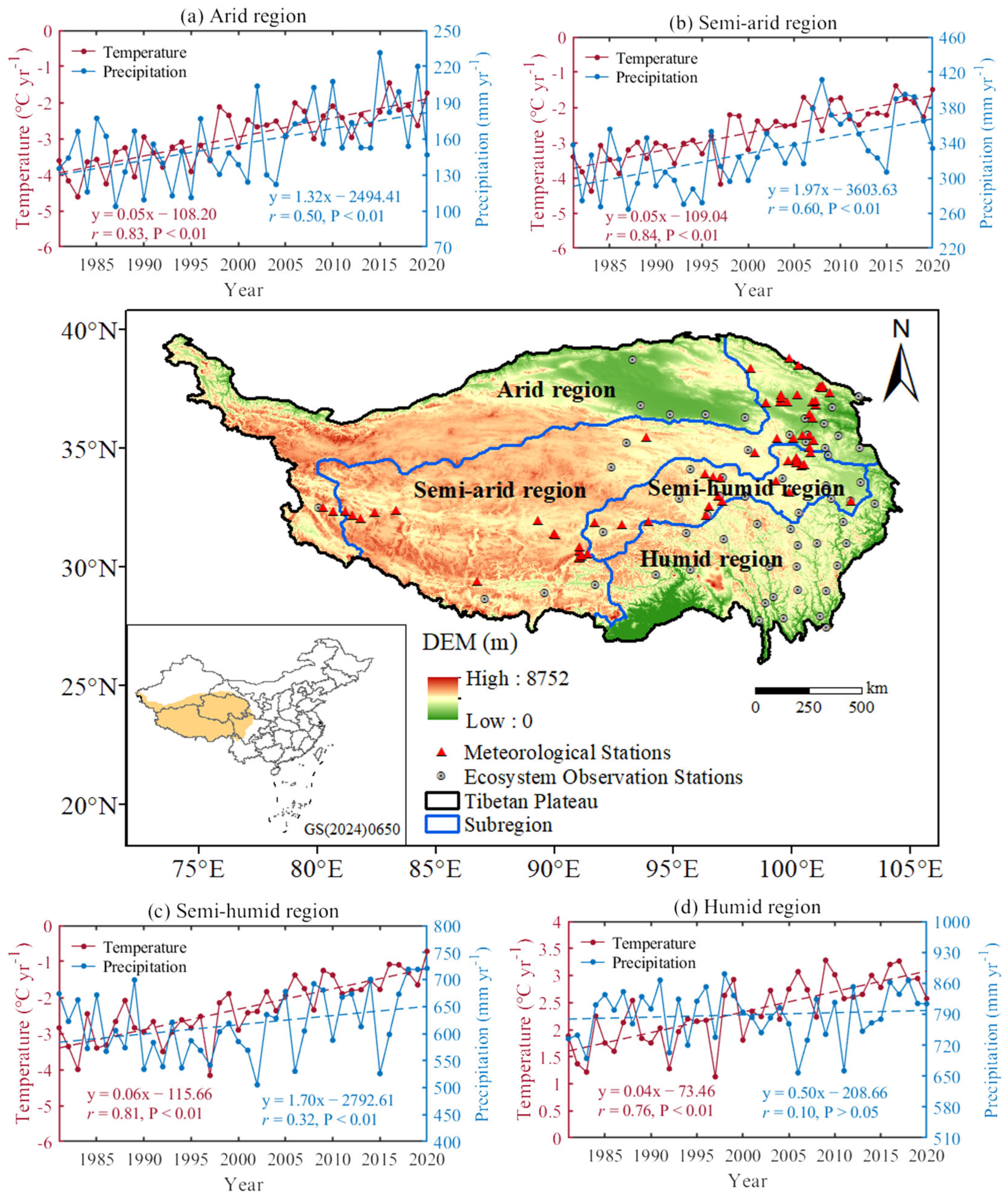
Figure 1. Patterns of wet and dry regions across the TP and interannual variations in key climatic factors within different moisture zones during 1981–2020. Red and blue dashed lines indicate the linear trends of temperature and precipitation, respectively.
Forests 17 00181 g001
Figure 2. Evaluation of LPJ model performance in simulating NPP and ET. (a) Relationship between observed and simulated NPP; (b) relationship between observed and simulated ET. Black dots denote paired observed and simulated values, the solid black line represents the 1:1 line, and the red line indicates the linear regression fit.
Forests 17 00181 g002
Figure 3. Spatial patterns of mean annual NPP and ET across the TP from satellite observations (a,c) and LPJ simulations (b,d) during 1982–2018.
Forests 17 00181 g003
Figure 4. Spatial patterns of temporal trends in NPP (a) and WY (c) across the TP during 1981–2020. Dots denote statistically significant trends (p < 0.05). Panels (b,d) show the longitudinal variations of mean NPP and WY trends estimated using the MMK test, respectively. Shaded areas represent the standard deviation.
Forests 17 00181 g004
Figure 5. Sensitivity of NPP and WY to climatic factors across the TP during 1981–2020. Results are shown for different moisture regions, including arid (I), semi-arid (II), semi-humid (III), humid (IV), and the entire TP (All).
Forests 17 00181 g005
Figure 6. Spatial patterns of mean annual climatic drivers across the TP during 1981–2020.
Forests 17 00181 g006
Figure 7. Spatial pattern of the rate of climate drivers across the TP during 1981–2020. Dots denote statistically significant trends (p < 0.05).
Forests 17 00181 g007
Figure 8. Temporal evolution of annual NPP and associated climatic and hydrological drivers across the TP during 1981–2020. (a) NPP and WY; (b) temperature and precipitation; (c) RAD and VPD; (d) SM. Red and blue dashed lines indicate the linear trends of the corresponding variables.
Forests 17 00181 g008
Figure 9. The q-values of environmental driving factors for NPP derived from the Geodetector analysis across the TP and its moisture subregions.
Forests 17 00181 g009
Figure 10. The q-values of interaction effects among environmental driving factors for NPP derived from the Geodetector interaction detector across the TP and its moisture subregions. Note: “*”and “**” indicate bi-variable-enhanced and nonlinear-enhanced interaction categories, respectively.
Forests 17 00181 g010
Figure 11. Taylor diagrams comparing observed and CMIP6 simulated temperature and precipitation across the TP during 1981–2014. Dotted lines indicate SD; dashed lines indicate centered RMSE differences; and dot-dash lines indicate correlations.
Forests 17 00181 g011
Figure 12. Spatial patterns of change rates in NPP and WY across the TP for the period 2015–2060 under different SSP scenarios. Dots denote statistically significant trends (p < 0.05).
Forests 17 00181 g012
Figure 13. Interannual variations of NPP anomalies (%) across four moisture subregions of the TP during 1981–2060. Shaded areas and grey bars show the mean ± 1 SD of ten CMIP6 models.
Forests 17 00181 g013
Figure 14. Interannual variations of WY anomalies (%) across four moisture subregions of the TP during 1981–2060. Shaded areas and grey bars show the mean ± 1 SD of ten CMIP6 models.
Forests 17 00181 g014
Table 1. Summary of datasets used in this study.
DatePeriodResolutionSource
Temperature, precipitation1981–20200.5° × 0.5°http://data.cma.cn, accessed on 12 January 2024
TerraClimate
(RAD, VPD, and SM)
1981–20201/24°https://www.climatologylab.org, accessed on 21 July 2024
GLASS (NPP, ET)1981–20200.05° × 0.05°http://www.glass.umd.edu/, accessed on 16 May 2024
CRU TS4.07
(cloud cover, humidity)
1981–20200.5° × 0.5°https://crudata.uea.ac.uk/cru/, accessed on 10 February 2024
Atmospheric CO2 concentration1981–2020/https://scrippsco2.ucsd.edu/, accessed on 28 February 2024
Soil data20091 kmhttp://data.tpdc.ac.cn, accessed on 17 January 2024
GCMs data1981–2060/https://esgf-node.llnl.gov/search/cmip6, accessed on 21 September 2024
Table 2. Types of interactions between two driving factors identified by Geodetector.
CriterionInteraction Types
q(Xi∩Xj) < Min(q(Xi), q(Xj))Nonlinear weaken
Min(q(Xi), q(Xj)) < q(Xi∩Xj) < Max(q(Xi), q(Xj))Uni-variable weaken
q(Xi∩Xj) > Max(q(Xi), q(Xj))Bi-variable enhancement
q(Xi∩Xj) = q(Xi) + q(Xj)Independent
q(Xi∩Xj) > q(Xi) + q(Xj)Nonlinear enhancement
Disclaimer/Publisher’s Note: The statements, opinions and data contained in all publications are solely those of the individual author(s) and contributor(s) and not of MDPI and/or the editor(s). MDPI and/or the editor(s) disclaim responsibility for any injury to people or property resulting from any ideas, methods, instructions or products referred to in the content.