Comparative Calculation of Spectral Indices for Post-Fire Changes Using UAV Visible/Thermal Infrared and JL1 Imagery in Jinyun Mountain, Chongqing, China

Abstract

This study used Jilin-1 satellite data and unmanned aerial vehicle (UAV)-collected visible-thermal infrared imagery to calculate twelve spectral indices and evaluate their effectiveness in distinguishing post-fire forest areas and identifying human-altered land-cover changes in Jinyun Mountain, Chongqing. The research goals included mapping wildfire impacts with M-statistic separability, measuring land-cover distinguishability through Jeffries–Matusita (JM) distance analysis, classifying land-cover types using the random forest (RF) algorithm, and verifying classification accuracy. Cumulative human disturbances—such as land clearing, replanting, and road construction—significantly blocked the natural recovery of burn scars, and during long-term human-assisted recovery periods over one year, the Red Green Blue Index (RGBI), Green Leaf Index (GLI), and Excess Green Index (EXG) showed high classification accuracy for six land-cover types: road, bare soil, deadwood, bamboo, broadleaf, and grass. Key accuracy measures showed producer accuracy (PA) > 0.8, user accuracy (UA) > 0.8, overall accuracy (OA) > 90%, and a kappa coefficient > 0.85. Validation results confirmed that visible-spectrum indices are good at distinguishing photosynthetic vegetation, thermal bands help identify artificial surfaces, and combined thermal-visible indices solve spectral confusion in deadwood recognition. Spectral indices provide high-precision quantitative evidence for monitoring post-fire land-cover changes, especially under human intervention, thus offering important data support for time-based modeling of post-fire forest recovery and improvement of ecological restoration plans.

1. Introduction

Wildfire disturbance poses significant challenges to forest management [1]. An accurate assessment of post-fire spectral index dynamics is critical for understanding ecosystem recovery mechanisms and guiding restoration practices [2]. Recent advancements in unmanned aerial vehicle (UAV) and satellite remote sensing technologies have enabled comprehensive characterization of forest fire scars [3], providing essential data to support post-fire reconstruction decisions and management strategy optimization [4,5].

Despite extensive validation of remote sensing spectral indices [6,7], effective tools for analyzing land-cover changes in fire scars—particularly anthropogenically disturbed burned areas—remain limited [8]. Representative indices include the following:

• The Burned Area Index (BAI), integrating visible and near-infrared bands [9,10];
• The Normalized Burn Ratio (NBR), incorporating short-wave infrared [11,12];
• The thermal infrared-enhanced Normalized Burn Ratio (NBRT) [13].

Additionally, spectral indices developed for RGB imagery demonstrate robust capabilities in vegetation identification and land-cover change detection, including the following:

• Simple band ratios (e.g., R/G, G/B) [14,15];
• Complex transformations (e.g., the Excess Green Index [EXG], Green Leaf Index [GLI], Triangular Greenness Index [TGI]) [16].

These RGB-based indices leverage ubiquitous visible-light imagery from multi-source platforms (UAVs, cameras, smartphones) [16], offering distinct operational advantages [17,18].

Fire scar dynamics encompass both natural vegetation recovery [2,19] and anthropogenic activities [8], such as land clearing, road construction, and artificial reforestation. Evaluating these processes requires the integrated application of

• Vegetation indices [19];
• Fire scar indices [11];
• Soil indices [20,21].

Post-fire surface residues progressively degrade due to environmental factors and human intervention [22,23], while concurrent vegetation regeneration drives scar evolution [5]. This regeneration correlates significantly with vegetation-specific spectral indices [24,25]. However, anthropogenic disturbances frequently induce abnormal fluctuations and uncertainties in these indices [26], necessitating optimization through feature transformation, zonal classification, or recalibration [27,28].

This study investigates anthropogenic restoration practices during the forest post-fire recovery process at Jinyun Mountain, Chongqing [19,29]. Using visible-thermal infrared imagery from a DJI Mavic 2 Enterprise Dual (M2D) UAV (was designed/manufactured by DJI Innovations in Shenzhen, China) and contemporaneous Jilin-1 (JL1) satellite data [28,30], we calculated twelve spectral indices to

• Assess accuracy in distinguishing burned areas [31,32];
• Identify anthropogenically disturbed land cover [8,27].

The evaluation encompassed four objectives:

• Delineating fire scars using M-statistic separability metrics [7];
• Quantifying land-cover separability via Jeffries–Matusita (JM) distance analysis [31,33];
• Classifying land cover with random forest (RF) [25,27];
• Validating accuracy [24,31,33].

This study focuses specifically on identifying and analyzing anthropogenic traces left after the fire. It examines their spectral characteristics in RGB bands using UAV imagery and compares them with high-resolution satellite imagery captured during a similar period. The goal is to systematically evaluate how well different spectral indices can distinguish between land-cover types within these altered areas, thereby providing a foundation for more accurate post-fire trace extraction.

2. Materials and Methods

2.1. Overview of Study Area and Technical Workflow

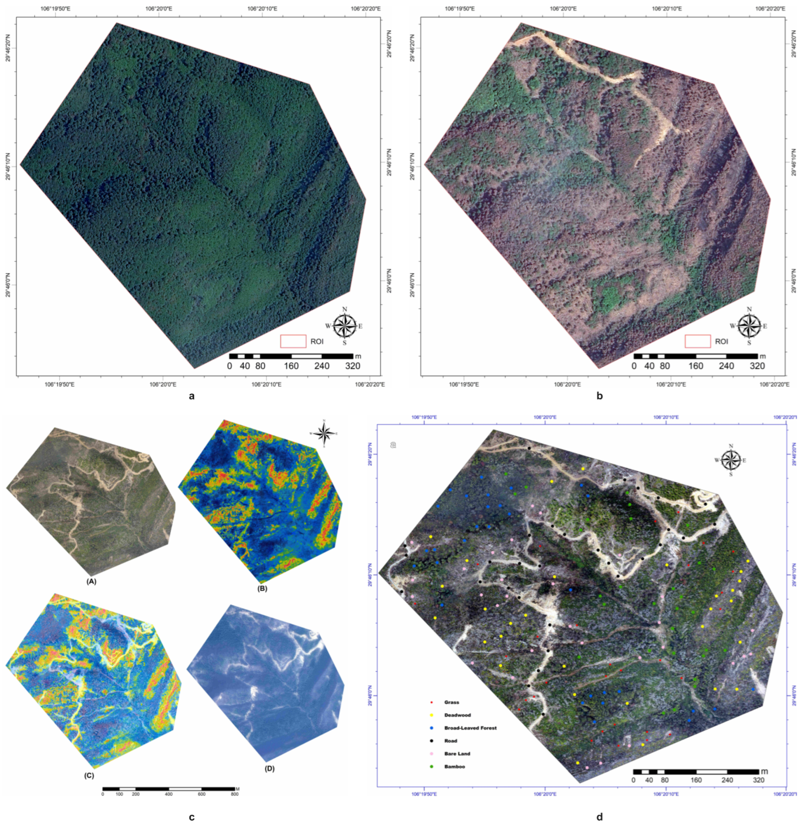
2.1.1. Study Area

The study area comprises the initial ignition zone of a forest fire that occurred from 21 to 26 August 2022 in the Jinyun Mountain Nature Reserve (106°19′–106°23′ E, 29°45′–29°49′ N; Figure 1), Beibei District, Chongqing [19,29]. Characterized by mountainous terrain under a subtropical humid monsoon climate, the reserve exhibits a mean annual temperature of 13.6 °C and annual precipitation of 1100 mm [25,26]. Dominant vegetation includes plantations of Pinus massoniana Lamb. and Cunninghamia lanceolata (Lamb.) Hook., with secondary evergreen broad-leaved forests. The understory is dominated by Lauraceae/Fagaceae-associated bamboos and shrubs, and herbaceous layers consist primarily of Asteraceae, Poaceae, and pteridophytes.

Triggered by temperatures exceeding 40 °C on 21 August 2022, the fire was contained within five days through integrated suppression strategies such as manual firebreak reinforcement, aerial water bombing, and controlled backfiring. Post-fire restoration initiatives involved planting fire-resistant species and enhancing infrastructure resilience, while recovery was monitored via UAV-based vegetation indices [2,20]. During the 2023 restoration programs, over 5000 volunteers planted native saplings across fire-affected zones [25].

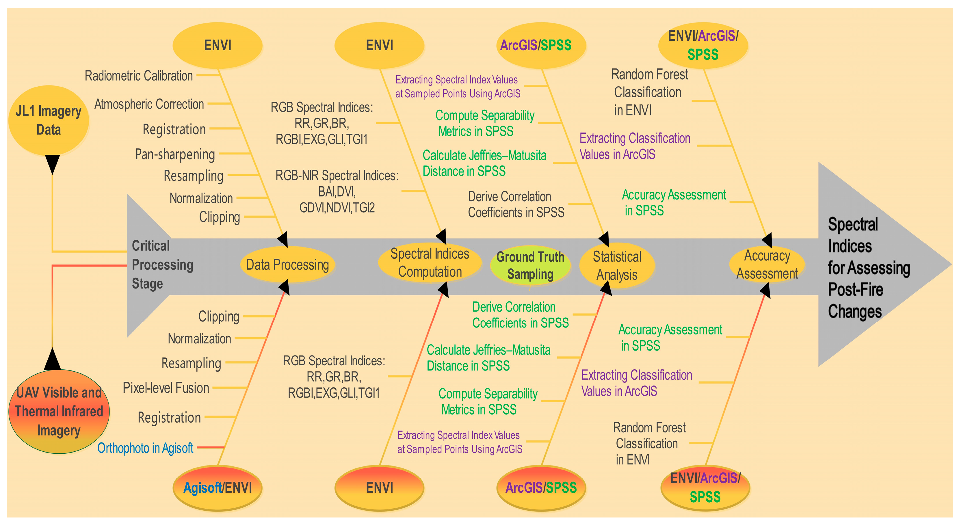
2.1.2. Technical Workflow

The framework (Figure 2) integrates five interconnected modules:

Data acquisition (Section 2.2.1): UAV dual-sensor (visible/thermal infrared) imagery (M2D; 28 December 2023) and JL1 satellite data (0.75 m resolution; 27 November 2023) were simultaneously acquired, supplemented by ground-truth sampling [4,5,20].

Data preprocessing (Section 2.2.2):

JL1 data: Radiometric calibration, atmospheric correction, co-registration, data fusion, resampling, and clipping were performed in ENVI v5.6.2 [6,7,20,34].

UAV data: Visible and thermal imagery were processed in Agisoft Metashape Pro v2.0.3 to generate orthomosaics [6,34], followed by co-registration, thermal-visible fusion, resampling, and clipping in ENVI [7,34].

Spectral index computation (Section 2.3): Spectral indices were calculated using the spectral index toolbox or raster calculator in ENVI [7,20,25,33], and then exported to ArcGIS v10.8.2 for analysis [11,23].

Statistical validation (Section 2.4): Statistical analyses encompassing correlation coefficients, discriminative metrics (M), and Jeffries–Matusita (JM) distance were computed in SPSS v30.0 [9,11,30].

Accuracy assessment (Section 2.5): Classification results from the random forest algorithm in ENVI were exported to ArcGIS for spatial refinement. Producer accuracy (PA), user accuracy (UA), overall accuracy (OA), and the kappa coefficient (kappa) were quantified in SPSS [2,11,23,35].

2.2. Image Data Acquisition and Preprocessing

2.2.1. Image Data Acquisition

At the burn scar site, UAV imagery was acquired on 28 December 2023 using a M2D equipped with visible-light and thermal infrared cameras (iron-red colormap) [14,36], concurrent with ground surveys [37]. A stratified random sampling design established 180 plots (3 m × 3 m) across six land-cover types: roads, bare soil, deadwood, bamboo, broadleaf, and grass (Figure 3d) [16,18,38].

Plot centroids were georeferenced using Trimble GeoXT receivers (<0.1 m horizontal accuracy) [37]. At 10–30 m above each plot centroid, the M2D acquired 6–10 nadir orthorectified images for validation [14,36].

JL1 images were obtained from the Jilin-1 official platform [20,39], with acquisition dates and specifications detailed in

Table 1. UAV and JL1 band information.

Bands	Channels	Wavelength/μm	Spatial Resolution/m	Acquisition Date	Satellite Sensor	Source
Pan		0.45~0.80	0.5/0.75	27 November 2023	JL1GF02B	https://www.jl1mall.com/ (Available from 12 August 2024 to 15 October 2024)
Band1	Blue	0.45~0.51	2/3	12 August 2024	JL1KF01B
Band2	Green	0.51~0.58		6 September 2022	JL1KF01C
Band3	Red	0.63~0.69		3 August 2022
Band4	NIR	0.77~0.895
RGB-V	Red/Green/Blue	0.40~0.70	0.07	28 December 2023	M2D visible sensor	This study
RGB-T	Red/Green/Blue	8~14	0.36	28 December 2023	M2D thermal infrared

-V represents visible light; -T represents thermal infrared. JL1GF02B: 0.75 m; JL1KF01B: 0.5 m; JL1KF01C: 0.5 m.

: 3 August and 6 September 2022 (JL1KF01C, 0.5 m), 27 November 2023 (JL1GF02B, 0.75 m), and 12 August 2024 (JL1KF01B, 0.5 m).

2.2.2. Image Preprocessing

UAV Image Processing: After orthomosaics were generated from quality-controlled UAV images in Agisoft Metashape v2.0.3, standardized ENVI v5.6.2 processing was conducted.

Geometric Registration: Thermal infrared imagery was registered to visible-light imagery as the spatial reference [15,35].

Thermal-Visible Fusion: Thermal infrared and visible red bands were fused using the Gram–Schmidt algorithm [34,40].

Resampling: Spatial resolution was standardized to 0.75 m via bilinear interpolation [23,39].

Data Normalization: The operation b1/255.0 was applied to convert DN values to the [0,1] reflectance range [37].

Cropping: Data were clipped to the study area ROI (Figure 1d) [16,34].

JL1 Satellite Image Processing: The standardized workflow comprised the following:

Radiometric Calibration: DN values were converted to reflectance using sensor-specific calibration coefficients [7,20].

Atmospheric Correction: Scattering/absorption effects were corrected with the FLAASH module (Mid-Latitude Summer model) [11,26].

Geometric Registration: Sub-pixel alignment (RMS < 0.5 pixels) was achieved relative to UAV orthomosaics [37,39].

Spatial Enhancement: Spatial resolution was enhanced through Gram–Schmidt pan-sharpening [26,40].

Resampling: Resolution was unified to 0.75 m via bilinear interpolation [23,39].

Data Normalization: The formula b1/10,000.0 was used to transform DN values into reflectance [20].

Cropping: ROI-based clipping was implemented (Figure 1d and Figure 3) [34].

2.3. Spectral Index Calculation

Resampled imagery was processed in ENVI to calculate spectral indices. UAV imagery spectral indices were computed using the Band Math toolbox ENVI v5.6.2 [5,28]. For JL1 data, the Burned Area Index (BAI), Difference Vegetation Index (DVI), Global DVI (GDVI), Normalized Difference Vegetation Index (NDVI), and Triangular Greenness Index 2 (TGI2) were calculated via the Spectral Index Calculation toolbox [7,24,31,41,42,43]. Remaining indices were computed using the Band Math toolbox [28]. A total of 12 spectral indices were calculated (

Table 2. Expressions for calculating spectral indices.

Index	Abbreviation	Expression	Reference
Red Ratio	RR	$R/(R+G+B)$	[32]
Green Ratio	GR	$G/(R+G+B)$	[32]
Blue Ratio	BR	$B/(R+G+B)$	[32]
Red/Green/Blue Index	RGBI	$(G^2-R\times B)/(G^2+R\times B)$	[25]
Excess Green	EXG	$2\times G-R-B$	[24]
Green Leaf Index	GLI	$\left(2\times G-R-B\right)/\left(2\times G+R+B\right)$	[41]
Triangular Greenness Index 1	TGI1	$G-0.39\times R-0.61\times B$	[44]
Triangular Greenness Index 2	TGI2	$$\begin{gathered} (\left({\lambda }_{RED}-{\lambda }_{BLUE}\right)\times ({\rho }_{RED}-{\rho }_{GREEN}) \\ -({\lambda }_{RED}-{\lambda }_{GREEN})\times ({\rho }_{RED}-{\rho }_{BLUE}))/2 \end{gathered}$$	[42]
Difference Vegetation Index	DVI	${\rho }_{NIR}-{\rho }_{RED}$	[38]
Green Difference Vegetation Index	GDVI	${\rho }_{NIR}-{\rho }_{GREEN}$	[30]
Normalized Difference Vegetation Index	NDVI	${(\rho }_{NIR}-{\rho }_{RED})/{(\rho }_{NIR}+{\rho }_{RED})$	[43]
Burned Area Index	BAI	$1/({(0.1-RED)}^2+{(0.06-NIR)}^2)$	[7]

RED (R), GREEN (G), BLUE (B), and NIR represent the reflectivity or normalized value of the red band, green band, blue band, and near-infrared band; λ represents the wavelength; and ρ represents the reflectivity.

). Pixel-level extraction was performed using ArcGIS [18,29].

2.4. Data Processing and Analysis

2.4.1. Distinguishing Indices

In SPSS, the discrimination index (M) was computed to quantitatively assess the spectral separability for post-fire land-cover classification, defined as [31,33,38]:

$$\mathrm{M}={\displaystyle \frac{\mu -\mu 0}{\sigma +\sigma 0}}$$

(1)

where μ and μ0 are the average spectral indices of the land type and the compared land, respectively, and σ and σ0 are the corresponding standard deviations. The larger the M value is, the easier it is to distinguish the land type from the contrasted land. In this case, M > 1 indicates good discrimination, and M < 1 indicates poor discrimination [9,11,23].

2.4.2. Jeffries–Matusita (JM) Distance

The Jeffries–Matusita (JM) distance is also commonly used to assess the separability of the two classes [11,23,40], which is calculated with Equation (2).

$$\mathrm{JM}=\sqrt{2\left(1-e^{\alpha }\right)}$$

(2)

$$\alpha ={\displaystyle \frac{1}{8}}{\left({\mu }_i-{\mu }_j\right)}^T{\left({\displaystyle \frac{C_i+C_j}{2}}\right)}^{-1}\left({\mu }_i-{\mu }_j\right)+{\displaystyle \frac{1}{2}}\mathit{ln}\left(\left|{\displaystyle \frac{\left|C_i+C_j\right|}{2\sqrt{\left|C_i\right|\times \left|C_j\right|}}}\right|\right)$$

(3)

where i and j are two categories; C is the variance of the categorical eigenvalues; and μ is the mean of the characteristic values of the category. The higher the JM value, the easier it is to distinguish the site features from the forest land. In this case, JM > 1 indicates good separability, and JM < 1 indicates poor separability [11,17].

2.4.3. Relevance

In SPSS, the covariance matrix and correlation coefficient matrix are generated by computing statistical measures for all pixel values derived from the image. This process enables the assessment of the linear correlation between variables using the Pearson correlation coefficient [10,11,37], $r_{xy}$, calculated as follows:

$$r_{xy}={\displaystyle \frac{{\sum }_{i=1}^n\left(x_i-\overline{x}\right)\left(y_i-\overline{y}\right)}{\sqrt{{{\sum }_{i=1}^n\left(x_i-\overline{x}\right)}^2}·\sqrt{{{\sum }_{i=1}^n\left(y_i-\overline{y}\right)}^2}}}$$

(4)

where $x_i$, $y_i$ are the values of two bands; $\overline{x},\overline{y}$ are the averages of the two bands; and $\lambda$ is the total number of pixels in the image.

2.5. Accuracy Evaluation

The random forest classification was performed on spectral indices from 180 field plots (144 training/36 validation) in ENVI v5.6.2 (100 trees, default parameters), with the results extracted to sample points in ArcGIS. SPSS was used to generate a confusion matrix, from which the overall accuracy (OA), kappa coefficient (kappa), producer accuracy (PA; omission error control), and user accuracy (UA; commission error control) were calculated [45].

3. Results

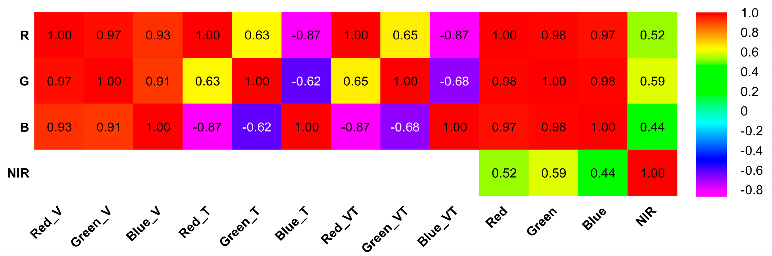
3.1. Spectral Band Comparison

Raw image bands in the study area underwent correlation analysis (Figure 4). For UAV visible bands, there were strong inter-band correlations (r > 0.9) among RGB channels; for UAV thermal band (8–14 μm) pseudocolor (iron-red palette) imagery, the blue channel exhibited negative correlations with the visible red (r = −0.87) and green bands (r = −0.62), where iron-red hues indicate elevated surface temperatures. There were high correlations (r > 0.95) for JL1 visible bands and low correlations (r < 0.6) for JL1 NIR vs. visible bands, enabling optimal band combinations for spectral enhancement.

3.2. Comparison of Distinguishing Indices

The spectral discrimination indices (M) were compared between UAV and JL1 imagery for pre-fire (3 August 2022) and post-fire (6 September 2022) scenarios (

Table 3. Discrimination (M) of different spectral indices.

Index	Pre-Fire (JL1-83)		JL1-96			JL1-27		JL1-812		UAV-V		UAV-T		UAV-VT
	Mean	STD	Mean	STD	M	M83	M96	M83	M96	M83	M96	M83	M96	M83	M96
RR	0.2354	0.0080	0.3394	0.0288	2.8252	2.0791	0.2985	2.4236	0.0723	5.0145	0.1690	0.3745	0.8441	0.1593	0.6919
GR	0.3797	0.0099	0.3342	0.0094	2.3585	1.2249	0.1724	0.8112	1.6797	1.0421	0.5855	0.0296	0.4474	0.1007	0.4061
BR	0.3849	0.0117	0.3264	0.0212	1.7803	1.1318	0.2598	6.4715	2.8322	2.4962	0.5538	0.3049	0.5318	0.1680	0.4228
RGBI	0.2280	0.0380	0.0065	0.0418	2.7736	1.4518	0.1729	0.7546	1.8912	1.2695	0.5819	1.1210	1.8623	0.4743	1.0486
EXG	0.0216	0.0057	0.0000	0.0059	1.8650	0.9334	0.1372	0.7498	1.5413	0.5847	0.8778	0.4910	0.5559	0.4220	0.4863
GLI	0.1007	0.0207	0.0018	0.0210	2.3672	1.2350	0.1652	0.7927	1.7044	1.0505	0.5875	0.0849	0.4079	0.1536	0.3729
TGI1	0.0083	0.0028	0.0004	0.0021	1.6018	0.7240	0.0881	1.2039	1.9514	0.7877	1.0091	0.2650	0.3054	0.2308	0.2709
BAI	38.5388	30.1057	161.2208	86.5482	1.0517	0.0938	1.1439	0.5757	1.4923
DVI	0.2049	0.0681	0.0669	0.0230	1.5156	0.0503	1.1111	0.6005	2.0382
GDVI	0.1826	0.0654	0.0688	0.0253	1.2552	0.0791	1.1287	0.7489	2.1332
NDVI	0.7228	0.0663	0.3115	0.0671	3.0831	0.8030	1.0378	0.0810	2.0397
TGI2	0.6851	0.2523	0.0503	0.1724	1.4947	0.6613	0.0720	1.3304	2.0627

JL1-83: JL1 image acquired on 3 August 2022; JL1-96: JL1 image acquired on 6 September 2022; JL1-27: JL1 image acquired on 27 November 2023; JL1-812: JL1 image acquired on 12 August 2024; UAV-V: UAV visible light imagery; UAV-T: UAV thermal infrared imagery; UAV-VT: fused UAV visible/thermal imagery; Mean: average value; STD: standard deviation; M83: discrimination index M using pre-fire reference (3 August 2022); M96: discrimination index M using post-fire reference (6 September 2022).

). Table 3 reveals three key findings: Immediate post-fire (11 days): Post-fire M values (JL1-96, M83) for all spectral indices exceeded 1, with the NDVI (M = 3.08) demonstrating the highest separability from pre-fire conditions and the BAI (M = 1.05) the lowest. This indicates NDVI is more sensitive to fire-induced vegetation changes. Long-term recovery (>1 year): Human activities (road construction/logging) showed divergent separability between pre- and post-fire baselines. For JL1-27, most indices had M < 1 (except EXG, TGI1, TGI2). Anomaly: Pre-fire M > 1 and post-fire M < 1. Sensor-specific responses: UAV-visible: the EXG (M < 1) showed reduced separability, while others inverted from M > 1 (pre-fire) to M < 1 (post-fire). UAV-thermal: Only the RGBI maintained M > 1 post-fire; the others had M < 1; see Table 3.

3.3. Comparison of Spectral Indices of Different Ground Objects

This study characterizes post-fire land-cover spectra by comparing average spectral index values (

Table 4. Mean spectral index.

Indices	Road	Bare Land	Deadwood	Grass	Bamboo	Broad-Leaved Forest
RR_V	0.372	0.360	0.346	0.359	0.344	0.341
GR_V	0.338	0.335	0.334	0.349	0.378	0.363
BR_V	0.291	0.305	0.320	0.292	0.278	0.296
RGBI_V	0.027	0.012	0.005	0.077	0.197	0.132
GLI_V	0.009	0.004	0.002	0.035	0.096	0.065
EXG_V	0.027	0.008	0.003	0.064	0.164	0.109
TGI1_V	0.033	0.014	0.005	0.042	0.092	0.061
RR_T	0.230	0.311	0.313	0.314	0.079	0.098
GR_T	0.457	0.369	0.414	0.412	0.350	0.285
BR_T	0.313	0.320	0.273	0.274	0.571	0.616
RGBI_T	0.718	0.436	0.542	0.560	0.497	0.220
GLI_T	0.246	0.058	0.156	0.152	0.029	−0.119
EXG_T	0.484	0.157	0.327	0.312	0.073	−0.078
TGI1_T	0.235	0.086	0.178	0.168	−0.022	−0.083
RR_VT	0.335	0.348	0.326	0.329	0.124	0.209
GR_VT	0.382	0.360	0.416	0.399	0.347	0.301
BR_VT	0.283	0.292	0.258	0.273	0.529	0.490
RGBI_VT	0.252	0.260	0.539	0.482	0.370	0.016
GLI_VT	0.104	0.048	0.161	0.129	0.023	−0.079
EXG_VT	0.356	0.140	0.321	0.292	0.055	−0.114
TGI1_VT	0.192	0.085	0.176	0.161	−0.026	−0.092
RR	0.397	0.347	0.340	0.331	0.319	0.315
GR	0.318	0.318	0.316	0.319	0.325	0.321
BR	0.285	0.335	0.345	0.350	0.356	0.363
RGBI	−0.053	−0.069	−0.079	−0.064	−0.034	−0.052
GLI	−0.035	−0.036	−0.040	−0.033	−0.018	−0.028
EXG	−0.028	−0.021	−0.023	−0.018	−0.010	−0.014
TGI1	−0.006	−0.010	−0.012	−0.010	−0.006	−0.009
TGI2	−0.301	−0.873	−1.058	−0.903	−0.620	−0.858
DVI	0.056	0.077	0.073	0.094	0.171	0.153
GDVI	0.107	0.091	0.084	0.100	0.168	0.151
NDVI	0.101	0.185	0.189	0.238	0.389	0.372

_V—visible light; _T—thermal infrared; and _VT—fused visible thermal infrared, which is not marked as JL1.

) from UAV and JL1-27 imagery.

Average EXG-V values for vegetation (bamboo = 0.164, broad-leaved forest = 0.109) significantly exceeded non-vegetation (road = 0.027, bare land = 0.008), confirming visible-light indices’ sensitivity to chlorophyll. EXG-V showed the highest discriminative power for live vegetation. The average RGBI-VT value for deadwood (0.539) was 107% higher than bare land (0.260) and 114% higher than roads (0.252), demonstrating that fused visible-thermal indices improve deadwood discrimination by integrating spectral and thermal features. Average NDVI values showed a strong positive correlation with vegetation cover (bamboo = 0.389, road = 0.101), aligning with ecological expectations. Conversely, indices like TGI2 exhibited universal negative average values (deadwood = −1.058), highlighting the need to optimize index formulas for sensor-specific spectral configurations.

To further explore the characteristics of spectral indices, violin plots (Figure 5) were used to visualize the distribution and central tendency of the data.

Analysis of the violin plots of indices across six types of land cover (road, bare land, deadwood, grass, bamboo, broadleaf) revealed the following key findings:

The RGBI-T of roads shows a right-skewed, compact distribution with a mean of 0.718, significantly higher than those of bamboo (0.497) and broadleaf (0.616), validating the impact of the high thermal emissivity of human-made materials on thermal indices.

Bamboo and broadleaf exhibit left-skewed BR-T distributions (mean values of 0.571 and 0.616, respectively), which are consistent with vegetation’s thermal radiation regulation through canopy transpiration.

For the RGBI-VT of deadwood, the mean (0.539) is 107% higher than that of bare land (0.260), suggesting that classification challenges posed by similar visible spectra can be resolved by integrating spectral and thermal features.

Grass shows a higher EXG-VT distribution dispersion (mean 0.289) than bamboo, reflecting high spectral variability in herbaceous vegetation.

Artificial surfaces (roads) exhibit right-skewed, peaked index distributions, while vegetation indices (e.g., BR-T) are left-skewed. Deadwood and bare land overlap in thermal indices but are separable via fused indices.

Significant inter-class mean differences (e.g., 44.5% between road RGBI-T and bamboo BR-T) provide visual evidence for fine-scale post-fire land-cover classification.

Violin plots effectively characterize the spectral index distributions across various types of land cover, confirming the superiority of thermal infrared indices in identifying artificial surfaces and the value of fused indices in deadwood mapping. This provides critical references for remote sensing-based fine-scale land-cover discrimination.

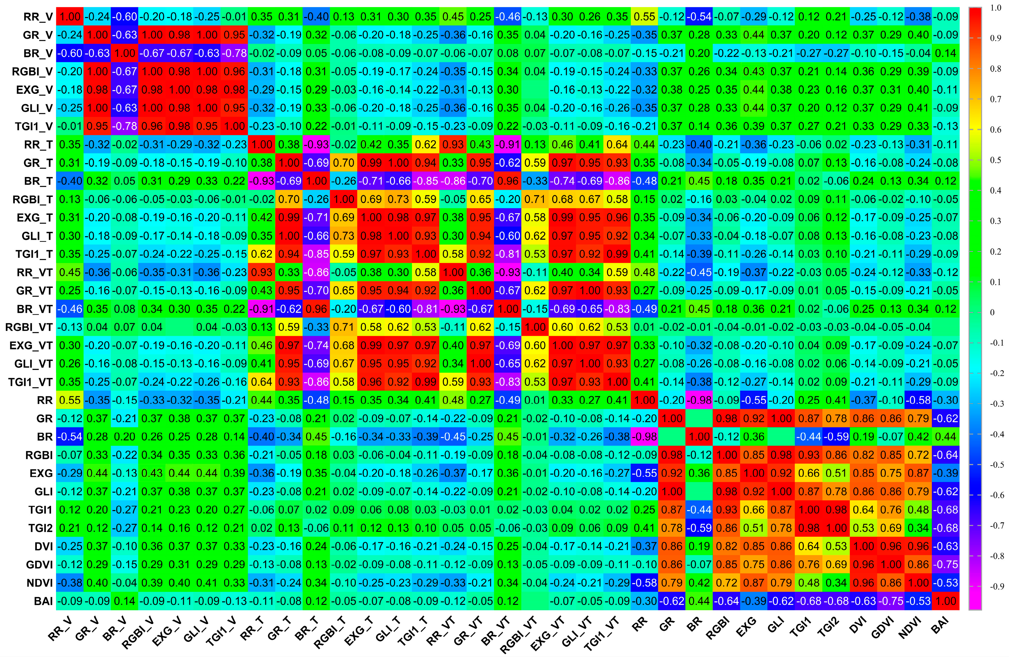
3.4. Correlation of UAVs with JL1-27 Spectral Index

To analyze the correlation between UAV and JL1-27 spectral indices, the correlation coefficients were calculated by statistically analyzing the index values of 180 sample plots (Figure 6).

This correlation matrix heatmap reveals index relationships, supporting the following core findings:

Single-band indices (visible/thermal infrared) show strong positive correlations (redundant functions). Cross-band indices have weak/negative correlations, enabling “spectral complementarity” (e.g., visible + thermal infrared) to enhance classification. This underpins the value of fused indices.

Fused indices (e.g., RGBI-VT) integrate dual-band information. They retain single-band sensitivity and resolve classification challenges for spectrally similar types of land cover (e.g., deadwood vs. bare land), validating their utility.

Special indices (e.g., TGI series) show weak negative correlations with others, adding classification details. However, indices such as TGI2 (with universal negative values) require formula optimization for sensor-specific spectra.

Using cross-band indices (weak correlation), simplifying redundant single-band indices, and leveraging special indices, scientific index combinations boost efficiency and accuracy in post-fire land-cover classification.

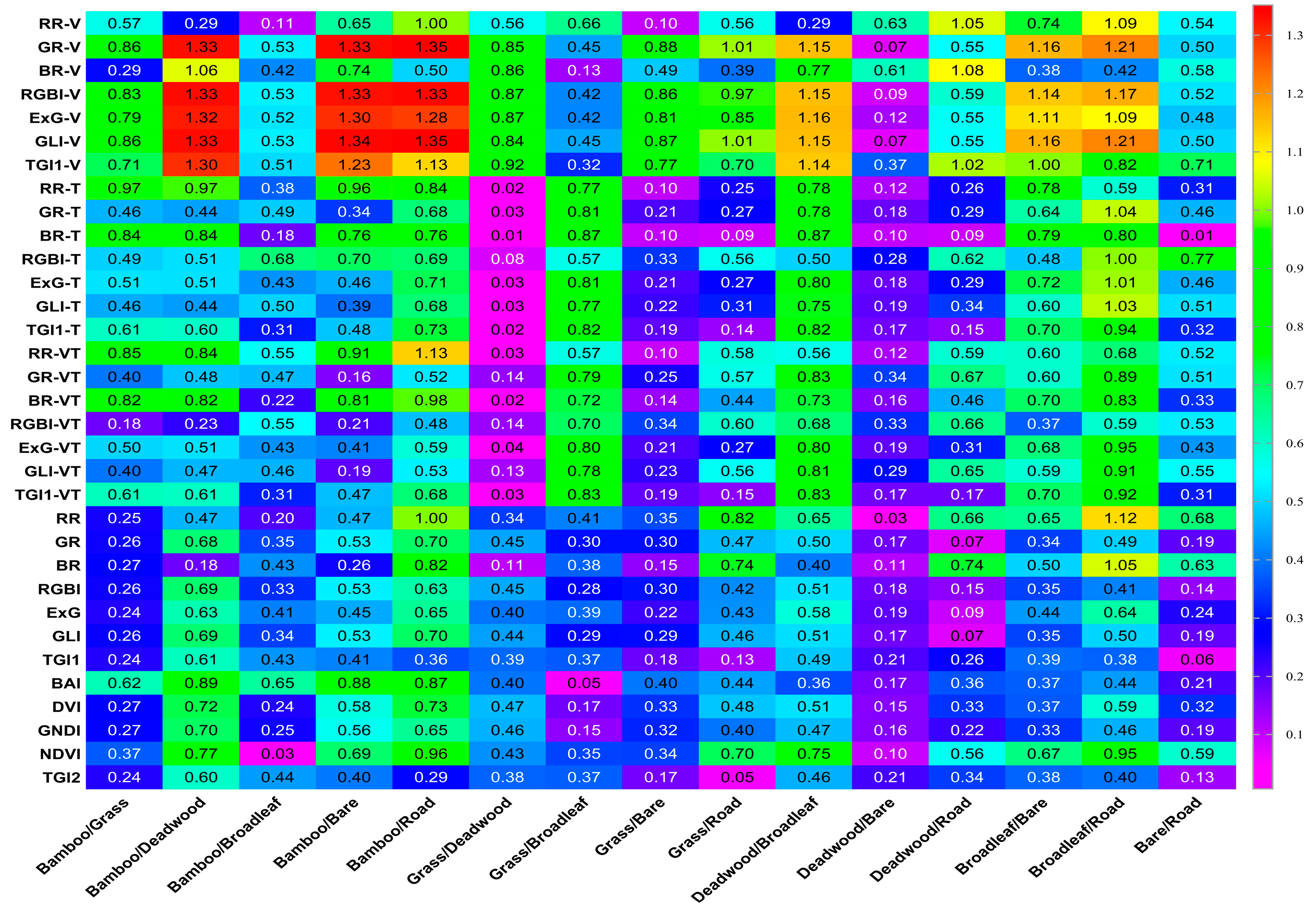
3.5. JM Distance and Spectral Indices

By integrating visible, thermal infrared, and fused spectral indices with original imagery, JM distances were calculated from 180 sample plots to evaluate the classification potential for six land-cover classes: grass, deadwood, bare land, road, bamboo, and broadleaf. To further understand the degree of differentiation of each index for each category, a random forest model was used to randomly select training samples and validation samples from 180 sample plots according to 80–20, of which 144 training samples were used for each land class and 36 validation samples were used to calculate the JM distance.

The heatmap (Figure 7) illustrates how all spectral indices, derived from original imagery, and JM distances quantify the separability of land-cover pairs (such as grass/road and deadwood/bare land). The guide to spectral index performance for land-cover pairs is based on the JM distance (Figure 8).

Thermal and fused indices (e.g., RGB-T, RGB-VT) strongly separate artificial surfaces (roads) from natural covers (grass, broadleaf). They are, thus, effective for identifying human-made areas.

Visible light indices (e.g., RGB-V) are better for distinguishing between vegetation types (grass vs. broadleaf/bamboo). They are, thus, useful for plant classes.

Fused indices (RGB-VT) work for both artificial/natural and vegetation/vegetation pairs. They are helpful for land covers that look similar in single bands (e.g., deadwood vs. bare land).

The JM Distance Spectral Index Ground Object Recognition Evaluation Guide (Figure 8) indicates the following:

Most of the spectral indices of UAV visible light show a large degree of discrimination (JM > 1) in distinguishing between bamboo and deadwood; bamboo and bare soil; bamboo and road; deadwood and broadleaf; broadleaf and bare soil; and broadleaf and road. That is, there is a significant distinction between living vegetation (bamboo, broadleaf) and non-living vegetation (road, deadwood, bare soil), as well as between non-vegetation types.

Most of the thermal infrared spectral indices and the spectral indices obtained by fusing thermal infrared with visible light exhibit a large degree of discrimination (JM > 0.7) in distinguishing between bamboo and road; grass and broadleaf; deadwood and broadleaf; and broadleaf and road. In other words, there is a notable distinction between living vegetation (bamboo, grass, broadleaf) and non-living vegetation (road, deadwood).

Most of the JL1 spectral indices demonstrate a large degree of discrimination (JM > 0.7) in distinguishing between bamboo and deadwood; bamboo and road; and broadleaf and road. That is, there is a significant distinction between living vegetation (bamboo, broadleaf) and non-living vegetation (road, deadwood).

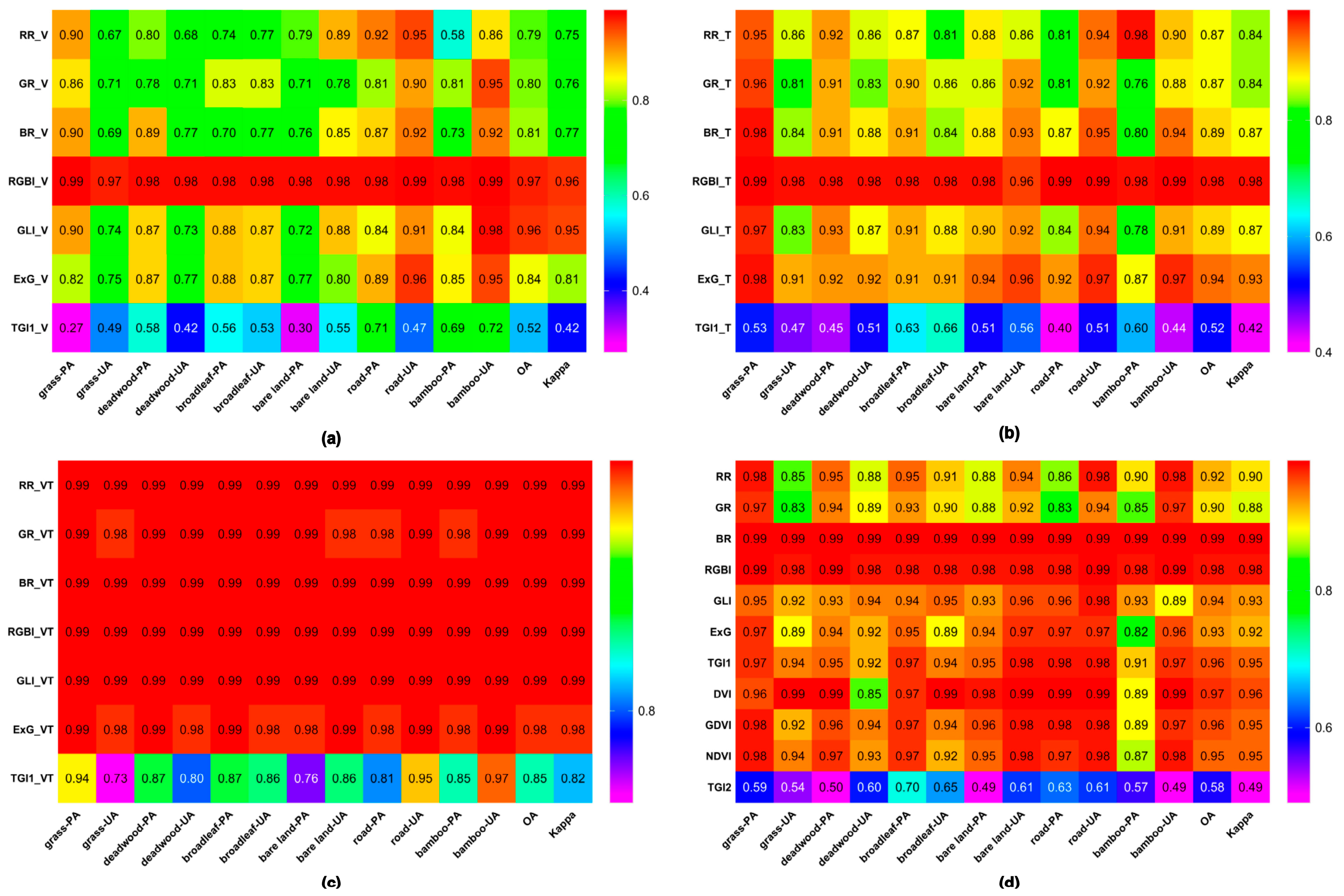
3.6. Accuracy Evaluation

To verify the accuracy of spectral indices, 180 field validation results were analyzed (Figure 9).

For UAV visible light spectral indices, the overall classification accuracy (OA) is close to or exceeds 80%, except for TGI1 (52%). Specifically, the RGBI and GLI exhibit accuracies exceeding 95%.

For UAV thermal infrared spectral indices, the overall classification accuracy is close to or exceeds 90%, except for TGI1 (52%). Notably, the RGBI (98%) and EXG (94%) demonstrate particularly high accuracies.

For JL1 spectral indices, the overall classification accuracy exceeds 90%, except for TGI2 (58%).

Other evaluation metrics (PA, UA, and kappa) show consistent trends with the overall classification accuracy (OA).

4. Discussion

4.1. Differences in the Extraction of Forest Fire Scars at the Pixel Scale Between UAV and JL1 Images

UAV RGB spectral indices demonstrate distinct advantages for vegetation identification, a finding consistent with multiple studies [16,37]. This research further validates their efficacy in distinguishing deadwood from bare ground. Integrating UAV thermal infrared imagery enhances feature differentiation through enriched spectral information, aligning with established thermal applications in forest fire scar analysis [14,36]. Although JL1 high-resolution satellite imagery is limited to four bands (R/G/B/NIR), it enables the extraction of >30 spectral indices from panchromatic (0.5 m/0.75 m) and multispectral (2 m/3 m) data [39]. Further investigation of these indices is warranted to assess their impact on forest fire scar dynamics, particularly deadwood distribution and early-stage natural vegetation recovery [2,14]. Such analysis is critical for optimizing UAV thermal/infrared and high-resolution satellite synergy in forest fire management [35].

4.2. Relationship Between Spectral Indices

UAV RGB bands exhibit autocorrelation, corroborating prior research [16]. Indices derived from these bands similarly display inter-correlation. Vegetation indices designed for plant identification also partially discriminate other land types, with RGB ratio indices demonstrating broad applicability. Thermal infrared pseudocolor gradation [46] significantly influences RGB spectral indices; the iron-red palette optimally represents forest fire scar dynamics, aligning with M2D thermal infrared methodologies [14,36]. In this study, thermal gradation was configured as iron-red, where elevated temperatures increase red values and decrease blue values, while lower temperatures augment blue values. Consequently, blue-band ratios exhibit negative correlations with temperature-sensitive indices.

Beyond pre-fire imagery [35], persistent fire remnants provide effective baselines for change assessment [45]. These exhibit opposing discriminative trends: pre-fire M > 1 versus post-fire M < 1. JL1-812 data revealed pronounced differentiation 11 days post-fire (RR > 1 excepted). UAV visible indices (excluding EXG and TGI1) and thermal/fused RR indices registered M < 1, potentially attributable to resolution disparities: pre-fire (0.5 m), post-fire (0.75 m), UAV visible (0.07 m), and UAV thermal (0.36 m). Resampling to 0.75 m for spatial uniformity may obscure fine-scale changes [34].

4.3. Advantages and Disadvantages of Ground Surveys, Unmanned Aerial Vehicles, and Satellite Imagery

Ground surveys yield precise surface data but are labor-intensive, time-consuming, and costly [38]. UAVs offer operational flexibility yet suffer limited spatial coverage per acquisition [5]. JL1 satellites deliver wide-area high-resolution imagery but lack timely data acquisition [30]. Integrating high-resolution satellites, UAVs, and targeted ground surveys remains the optimal approach for comprehensive forest fire scar assessment [35].

5. Conclusions

In this study, the spectral indices of three living vegetation types (bamboo, broadleaf trees, grass), two non-vegetation classes (roads, bare soil), and deadwood in human-intervened post-fire environments were analyzed using ultra-high-resolution UAV visible/thermal infrared and Jilin-1 satellite data, employing the spectral discrimination index (M), JM distance, and random forest modeling [11,27,31]. The key findings demonstrate significant negative correlations (r > 0.7, p < 0.01) in UAV thermal pseudocolor imagery (iron-red gradation) among low-temperature (blue band), high-temperature (red band), and mid-temperature zones (green band), while JL1 near-infrared (NIR) exhibits a weak correlation with RGB bands (r < 0.6), providing a foundation for novel spectral index construction [16,17,37]. In the early post-fire stage (6 September 2022), all 12 spectral indices outperformed the BAI in separability (M-index) from the pre-fire forest (3 August 2022), with the NDVI achieving peak discrimination (M = 3.08) versus the BAI minimum (M = 1.05) [12,31]. During human-managed recovery (>1 year post 27 November 2023), visible light indices achieved a JM > 0.5 across six land-cover classes with critical distinction (JM > 1) between living vegetation (bamboo/broadleaf) and non-vegetation (roads/deadwood/bare soil), while thermal/visible fusion enhanced deadwood recognition accuracy by 107%, with optimal combinations yielding an overall accuracy of >90% (kappa > 0.85) [14,25,36]. Field validation confirms that pre-/post-fire separability (M-index) benchmarks detect latent land-cover transitions: a low M relative to pre-fire indicates living vegetation recovery, whereas a low M relative to early post-fire suggests non-vegetation dominance, with UAV dual-camera (visible/thermal) imagery demonstrating superior transitional-state sensitivity [24,39]. Correlating UAV-satellite spectral indices is critical for quantifying anthropogenic impacts (road engineering, deadwood removal, replanting) on vegetation reassembly, forest thermal/hydrological rebalancing, and landscape resilience trajectories [19,29,32].

References

1. Han, Y.; Zheng, C.; Liu, X.; Tian, Y.; Dong, Z. Burned Area and Burn Severity Mapping with a Transformer-Based Change Detection Model. IEEE J. Sel. Top. Appl. Earth Obs. Remote Sens. 2024, 17, 13866–13880. [Google Scholar] [CrossRef]
2. Zhang, L.; Wang, M.; Fu, Y.; Ding, Y. A Forest Fire Recognition Method Using UAV Images Based on Transfer Learning. Forests 2022, 13, 975. [Google Scholar] [CrossRef]
3. Xu, Y.; Li, J.; Zhang, F. A UAV-Based Forest Fire Patrol Path Planning Strategy. Forests 2022, 13, 1952. [Google Scholar] [CrossRef]
4. Li, X.; Gao, H.; Zhang, M.; Zhang, S.; Gao, Z.; Liu, J.; Sun, S.; Hu, T.; Sun, L. Prediction of Forest Fire Spread Rate Using UAV Images and an LSTM Model Considering the Interaction between Fire and Wind. Remote Sens. 2021, 13, 4325. [Google Scholar] [CrossRef]
5. Larrinaga, A.R.; Brotons, L. Greenness Indices from a Low-Cost UAV Imagery as Tools for Monitoring Post-Fire Forest Recovery. Drones 2019, 3, 6. [Google Scholar] [CrossRef]
6. Guimaraes, N.; Padua, L.; Marques, P.; Silva, N.; Peres, E.; Sousa, J.J. Forestry Remote Sensing from Unmanned Aerial Vehicles: A Review Focusing on the Data, Processing and Potentialities. Remote Sens. 2020, 12, 1046. [Google Scholar] [CrossRef]
7. Chuvieco, E.; Martín, M.P.; Palacios, A. Assessment of different spectral indices in the red-near-infrared spectral domain for burned land discrimination. Int. J. Remote Sens. 2002, 23, 5103–5110. [Google Scholar] [CrossRef]
8. Fraser, R.H.; van der Sluijs, J.; Hall, R.J. Calibrating Satellite-Based Indices of Burn Severity from UAV-Derived Metrics of a Burned Boreal Forest in NWT, Canada. Remote Sens. 2017, 9, 279. [Google Scholar] [CrossRef]
9. Quintano, C.; Fernandez-Manso, A.; Stein, A.; Bijker, W. Estimation of area burned by forest fires in Mediterranean countries: A remote sensing data mining perspective. For. Ecol. Manag. 2011, 262, 1597–1607. [Google Scholar] [CrossRef]
10. Perez, C.C.; Olthoff, A.E.; Hernandez-Trejo, H.; Rullan-Silva, C.D. Evaluating the best spectral indices for burned areas in the tropical Pantanos de Centla Biosphere Reserve, Southeastern Mexico. Remote Sens. Appl. Soc. Environ. 2022, 25, 100664. [Google Scholar] [CrossRef]
11. Pacheco, A.d.P.; da Silva, J.A., Jr.; Ruiz-Armenteros, A.M.; Henriques, R.F.F.; Santos, I.d.O. Analysis of Spectral Separability for Detecting Burned Areas Using Landsat-8 OLI/TIRS Images under Different Biomes in Brazil and Portugal. Forests 2023, 14, 663. [Google Scholar] [CrossRef]
12. Ji, X.; Zhou, Z.; Gouda, M.; Zhang, W.; He, Y.; Ye, G.; Li, X. A novel labor-free method for isolating crop leaf pixels from RGB imagery: Generating labels via a topological strategy. Comput. Electron. Agric. 2024, 218, 108631. [Google Scholar] [CrossRef]
13. Roy, D.R.; Boschetti, L.; Trigg, S.N. Remote sensing of fire severity: Assessing the performance of the normalized Burn ratio. IEEE Geosci. Remote Sens. Lett. 2006, 3, 112–116. [Google Scholar] [CrossRef]
14. Burnett, J.D.; Wing, M.G. A low-cost near-infrared digital camera for fire detection and monitoring. Int. J. Remote Sens. 2018, 39, 741–753. [Google Scholar] [CrossRef]
15. Kedia, A.C.; Kapos, B.; Liao, S.; Draper, J.; Eddinger, J.; Updike, C.; Frazier, A.E. An Integrated Spectral-Structural Workflow for Invasive Vegetation Mapping in an Arid Region Using Drones. Drones 2021, 5, 19. [Google Scholar] [CrossRef]
16. Trencanova, B.; Proenca, V.; Bernardino, A. Development of Semantic Maps of Vegetation Cover from UAV Images to Support Planning and Management in Fine-Grained Fire-Prone Landscapes. Remote Sens. 2022, 14, 1262. [Google Scholar] [CrossRef]
17. Mpakairi, K.S.; Kadzunge, S.L.; Ndaimani, H. Testing the utility of the blue spectral region in burned area mapping: Insights from savanna wildfires. Remote Sens. Appl. Soc. Environ. 2020, 20, 100365. [Google Scholar] [CrossRef]
18. Xiao, W.; Deng, X.; He, T.; Guo, J. Using POI and time series Landsat data to identify and rebuilt surface mining, vegetation disturbance and land reclamation process based on Google Earth Engine. J. Environ. Manag. 2023, 327, 116920. [Google Scholar] [CrossRef]
19. Ji, S.; Wang, Y.; He, L.; Zhang, Z.; Meng, F.; Li, X.; Chen, Y.; Wang, D.; Gong, Z. Greenhouse gas emission in the whole process of forest fire including rescue: A case of forest fire in Beibei District of Chongqing. Environ. Sci. Pollut. Res. 2023, 30, 113105–113117. [Google Scholar] [CrossRef]
20. Fu, B.; Zuo, P.; Liu, M.; Lan, G.; He, H.; Lao, Z.; Zhang, Y.; Fan, D.; Gao, E. Classifying vegetation communities karst wetland synergistic use of image fusion and object-based machine learning algorithm with Jilin-1 and UAV multispectral images. Ecol. Indic. 2022, 140, 108989. [Google Scholar] [CrossRef]
21. Beltran-Marcos, D.; Suarez-Seoane, S.; Fernandez-Guisuraga, J.M.; Fernandez-Garcia, V.; Marcos, E.; Calvo, L. Relevance of UAV and sentinel-2 data fusion for estimating topsoil organic carbon after forest fire. Geoderma 2023, 430, 116290. [Google Scholar] [CrossRef]
22. Udelhoven, T. TimeStats: A Software Tool for the Retrieval of Temporal Patterns from Global Satellite Archives. IEEE J. Sel. Top. Appl. Earth Obs. Remote Sens. 2011, 4, 310–317. [Google Scholar] [CrossRef]
23. Wu, B.; Zheng, H.; Xu, Z.; Wu, Z.; Zhao, Y. Forest Burned Area Detection Using a Novel Spectral Index Based on Multi-Objective Optimization. Forests 2022, 13, 1787. [Google Scholar] [CrossRef]
24. Woebbecke, D.M.; Meyer, G.E.; Vonbargen, K.; Mortensen, D.A. Color indexes for weed identification under various soil, residue, and lighting conditions. Trans. ASAE 1995, 38, 259–269. [Google Scholar] [CrossRef]
25. Bendig, J.; Yu, K.; Aasen, H.; Bolten, A.; Bennertz, S.; Broscheit, J.; Gnyp, M.L.; Bareth, G. Combining UAV-based plant height from crop surface models, visible, and near infrared vegetation indices for biomass monitoring in barley. Int. J. Appl. Earth Obs. Geoinf. 2015, 39, 79–87. [Google Scholar] [CrossRef]
26. Ma, D.; Wang, Q.; Huang, Q.; Lin, Z.; Yan, Y. Spatio-Temporal Evolution of Vegetation Coverage and Eco-Environmental Quality and Their Coupling Relationship: A Case Study of Southwestern Shandong Province, China. Forests 2024, 15, 1200. [Google Scholar] [CrossRef]
27. Kaufman, Y.J.; Remer, L.A. Detection of forests using mid-IR reflectance: An application for aerosol studies. IEEE Trans. Geosci. Remote Sens. 1994, 32, 672–683. [Google Scholar] [CrossRef]
28. Hao, P.; Zhan, Y.; Wang, L.; Niu, Z.; Shakir, M. Feature Selection of Time Series MODIS Data for Early Crop Classification Using Random Forest: A Case Study in Kansas, USA. Remote Sens. 2015, 7, 5347–5369. [Google Scholar] [CrossRef]
29. Zhao, Y.; Huang, Y.; Sun, X.; Dong, G.; Li, Y.; Ma, M. Forest Fire Mapping Using Multi-Source Remote Sensing Data: A Case Study in Chongqing. Remote Sens. 2023, 15, 2323. [Google Scholar] [CrossRef]
30. Sripada, R.P. Determining In-Season Nitrogen Requirements for Corn Using Aerial Color-Infrared Photography. Ph.D. Thesis, North Carolina State University, Raleigh, NC, USA, 2005. [Google Scholar]
31. Vargas-Sanabria, D.; Campos-Vargas, C. Multitemporal comparison of burned areas in a tropical dry forest using the burned area index (BAI). Rev. For. Mesoam. Kuru-Rfmk 2020, 17, 29–36. [Google Scholar] [CrossRef]
32. Richardson, A.D.; Jenkins, J.P.; Braswell, B.H.; Hollinger, D.Y.; Ollinger, S.V.; Smith, M.-L. Use of digital webcam images to track spring green-up in a deciduous broadleaf forest. Oecologia 2007, 152, 323–334. [Google Scholar] [CrossRef] [PubMed]
33. Pereira, J.M.C.; Mota, B.; Privette, J.L.; Caylor, K.K.; Silva, J.M.N.; Sá, A.C.L.; Ni-Meister, W. A simulation analysis of the detectability of understory burns in miombo woodlands. Remote Sens. Environ. 2004, 93, 296–310. [Google Scholar] [CrossRef]
34. Carvajal-Ramirez, F.; Marques da Silva, J.R.; Aguera-Vega, F.; Martinez-Carricondo, P.; Serrano, J.; Jesus Moral, F. Evaluation of Fire Severity Indices Based on Pre- and Post-Fire Multispectral Imagery Sensed from UAV. Remote Sens. 2019, 11, 993. [Google Scholar] [CrossRef]
35. Padua, L.; Guimaraes, N.; Adao, T.; Sousa, A.; Peres, E.; Sousa, J.J. Effectiveness of Sentinel-2 in Multi-Temporal Post-Fire Monitoring When Compared with UAV Imagery. ISPRS Int. J. Geo-Inf. 2020, 9, 225. [Google Scholar] [CrossRef]
36. Hendel, I.-G.; Ross, G.M. Efficacy of Remote Sensing in Early Forest Fire Detection: A Thermal Sensor Comparison. Can. J. Remote Sens. 2020, 46, 414–428. [Google Scholar] [CrossRef]
37. de Jesus Marcial-Pablo, M.; Gonzalez-Sanchez, A.; Ivan Jimenez-Jimenez, S.; Ernesto Ontiveros-Capurata, R.; Ojeda-Bustamante, W. Estimation of vegetation fraction using RGB and multispectral images from UAV. Int. J. Remote Sens. 2019, 40, 420–438. [Google Scholar] [CrossRef]
38. Tucker, C.J. Red and photographic infrared linear combinations for monitoring vegetation. Remote Sens. Environ. 1979, 8, 127–150. [Google Scholar] [CrossRef]
39. Sun, J.; Zhu, R.; Gong, J.; Qu, C.; Guo, F. Cross-Comparison Between Jilin-1GF03B and Sentinel-2 Multi-Spectral Measurements and Phenological Monitors. IEEE Access 2024, 12, 43540–43551. [Google Scholar] [CrossRef]
40. Zhang, X.; Sun, Y.; Shang, K.; Zhang, L.; Wang, S. Crop Classification Based on Feature Band Set Construction and Object-Oriented Approach Using Hyperspectral Images. IEEE J. Sel. Top. Appl. Earth Obs. Remote Sens. 2016, 9, 4117–4128. [Google Scholar] [CrossRef]
41. Louhaichi, M.; Borman, M.M.; Johnson, D.E. Spatially located platform and aerial photography for documentation of grazing impacts on wheat. Geocarto Int. 2001, 16, 65–70. [Google Scholar] [CrossRef]
42. Hunt, E.R., Jr.; Daughtry, C.S.T.; Eitel, J.U.H.; Long, D.S. Remote sensing leaf chlorophyll content using a visible band index. Agron. J. 2011, 103, 1090–1099. [Google Scholar] [CrossRef]
43. Rouse, J.W.; Haas, R.H.; Schell, J.A.; Deering, D.W. Monitoring vegetation systems in the great plains with ERTS. In Proceedings of the 3rd Earth Resources Technology Satellite Symposium, Washington, DC, USA, 10–14 December 1973. [Google Scholar]
44. Hunt, E.R., Jr.; Doraiswamy, P.C.; McMurtrey, J.E.; Daughtry, C.S.T.; Perry, E.M.; Akhmedov, B. A visible band index for remote sensing leaf chlorophyll content at the canopy scale. Int. J. Appl. Earth Obs. Geoinf. 2013, 21, 103–112. [Google Scholar] [CrossRef]
45. Bourgoin, C.; Betbeder, J.; Couteron, P.; Blanc, L.; Dessard, H.; Oszwald, J.; Le Roux, R.; Cornu, G.; Reymondin, L.; Mazzei, L.; et al. UAV-based canopy textures assess changes in forest structure from long-term degradation. Ecol. Indic. 2020, 115, 106386. [Google Scholar] [CrossRef]
46. Alpar, O.; Krejcar, O. Quantization and Equalization of Pseudocolor Images in Hand Thermography. In Bioinformatics and Biomedical Engineering, Proceedings of the IWBBIO 2017, Granada, Spain, 26–28 April 2017, Part I; Rojas, I., Ortuno, F., Eds.; Lecture Notes in Bioinformatics; Springer: Cham, Switzerland, 2017; Volume 10208, pp. 397–407. [Google Scholar]
Figure 1. Location maps: (a) within China; (b) Chongqing; (c) Jinyun Mountain Nature Reserve; (d) the Region of Interest (ROI).
Forests 16 01147 g001
Figure 2. Spectral analysis workflow.
Forests 16 01147 g002
Figure 3. UAV and JL1 imagery. (a) JL1 (3 August 2022); (b) JL1 (6 September 2022); (c) (28 December 2023); (A) UAV visible; (B) UAV thermal; (C) UAV fusion; (D) JL1 (27 November 2023); (d) sample points.
Forests 16 01147 g003
Figure 4. Band correlation. R—red band; G—green band; B—blue band; NIR—near-infrared band; _V—visible light; _T—thermal infrared; and _VT—fused visible thermal infrared, which is not marked as JL1.
Forests 16 01147 g004
Figure 5. Spectral index violin line. (a) _V—visible light; (b) _T —thermal infrared; and (c) _VT—fused visible thermal infrared, (d) which is not marked as JL1.
Forests 16 01147 g005
Figure 6. Correlation of spectral indices. _V—visible light; _T—thermal infrared; and _VT—fused visible thermal infrared, which is not marked as JL1.
Forests 16 01147 g006
Figure 7. JM distance of land-cover pairs for all spectral indices derived from original imagery. RGB-V: Visible Light Image; Index-V: Visible Light Spectral Index Set; RGB-T: Thermal Infrared Image; Index-T: Thermal Infrared Spectral Index Set; RGB-VT: Thermal Infrared Fusion Image; Index-VT: Thermal Infrared Fusion Spectral Index Set; JL1: JL1 Multispectral Image (27 November 2023); JL1Index: JL1 Spectral Index Set (27 November 2023).
Forests 16 01147 g007
Figure 8. Spectral index performance guide for land-cover pairs based on JM distance. _V—visible light; _T—thermal infrared; and _VT—fused visible thermal infrared, which is not marked as JL1.
Forests 16 01147 g008
Figure 9. Evaluation of spectrum indices classification accuracy. (a) Visible light; (b) thermal infrared; (c) thermal-visible fusion; (d) jl1. _V—visible light; _T—thermal infrared; _VT—thermal-visible fusion, which is not marked as JL1.
Forests 16 01147 g009