Rapid Large-Scale Monitoring of Pine Wilt Disease Using Sentinel-1/2 Images in GEE

Abstract

Pine wilt disease (PWD) is a severe forest disease caused by the infestation of pine wood nematodes. Due to its short disease cycle and strong transmission ability, it has caused significant damage to China’s forestry resources. To achieve large-scale monitoring of PWD, this study utilized machine learning/deep learning algorithms with Sentinel-1/2 images in the Google Earth Engine cloud platform to implement province-wide PWD monitoring in Anhui Province, China. The study also analyzed the spatial distribution of PWD in Anhui Province from two perspectives—spatiotemporal patterns and influencing factors—aiming to investigate the spatiotemporal evolution patterns and the impact of influencing factors on the occurrence of PWD. The results show that (1) the random forest model exhibited the strongest performance, followed by the CNN model, while the DNN model performed the worst. Using the RF model to monitor PWD and calculate the affected area in Anhui Province from 2019 to 2024 yielded errors within 30% compared to official statistics. (2) PWD in Anhui Province showed a clear clustering trend, with global Moran’s indices all exceeding 0.79 from 2019 to 2024. The LISA map revealed a spread pattern from south to north and from west to east. (3) Topographic and temperature factors had the greatest influence on PWD distribution. SHAP analysis indicated that topographic and climatic factors were the primary drivers of PWD-affected areas, with slope and temperature being the two most significant contributing factors. This study helps to rapidly and accurately identify outbreak areas during epidemics and enables precise quarantine measures and targeted control efforts.

1. Introduction

Pine wilt disease (PWD) is a forest disease transmitted by insect vectors and currently ranks among the most devastating forest diseases in China [1,2]. PWD was first detected in Nanjing, Jiangsu Province, China, in 1982. Characterized by rapid spread and being very difficult to control, the early and accurate identification of infected pine trees serves as a critical measure to prevent epidemic expansion [3].

In recent years, the development of remote sensing technology has provided crucial support for early monitoring of PWD [4], with research primarily focusing on the following two aspects: PWD characteristic studies and extraction algorithms. Early research on PWD characteristics mainly concentrated on physicochemical property changes and morphological alterations in infected trees, such as reduced water content, decreased chlorophyll concentration, and the gradual discoloration of canopies to reddish-brown. Traditional methods for identifying infected trees relied heavily on manual field surveys, which often missed optimal monitoring windows and subsequently increased control costs. Currently, remote sensing has emerged as a mainstream approach for detecting infected trees. Consequently, PWD characteristic research has increasingly focused on spectral feature variations caused by infection and the derived remote sensing indices. Following PWD infection, pine trees undergo significant physiological and biochemical changes [1], including chlorophyll degradation, water loss, and canopy color alteration [5]. Remote sensing vegetation indices have proven effective in distinguishing infected from healthy trees by capitalizing on these physicochemical changes, particularly reduced water content and altered canopy color, thereby achieving superior monitoring results [6]. Additionally, texture features and radar data have been employed for PWD identification [7,8]. For instance, Wang et al. achieved superior results using LiDAR point cloud data compared to hyperspectral imaging, and the fusion of LiDAR point clouds with hyperspectral data can accurately reflect the distribution of individual trees and their infection status [2,9]. Similarly, Yu et al. achieved better monitoring results by combining airborne LiDAR data with hyperspectral data compared to using either dataset alone, with LiDAR proving particularly effective in identifying deadwood [10].

Current forest remote sensing monitoring methods can be categorized into the following five major types: mathematical statistics, geostatistics, machine learning [11], expert systems, and fuzzy mathematics [12,13]. While these approaches have been extensively studied at regional scales, they still exhibit limitations. To address these challenges effectively, Hinton proposed the concept of deep learning [14]. PWD monitoring can be classified into scene-level, object-level, and pixel-level monitoring. For instance, Tao et al. conducted scene-level PWD remote sensing monitoring using deep learning techniques [15], comparing the performance of AlexNet, GoogLeNet, and template matching (TM) methods in detecting dead pine trees. Their findings demonstrated that convolutional neural networks significantly outperformed traditional TM methods in recognition accuracy. Object detection algorithms primarily fall into two categories: single-stage detection algorithms based on regression concepts and two-stage detection algorithms based on region proposal classification approaches [16,17]. Researchers like Li et al. designed a lightweight three-layer output YOLOv4-Tiny network architecture [18]. By reducing model complexity, this approach significantly improved computational efficiency while maintaining detection performance, achieving satisfactory recognition results. Park et al. developed an improved Faster R-CNN detection model based on the VGG-16 backbone architecture integrated with a Region Proposal Network (RPN) [19]. By optimizing the collaborative mechanism between feature extraction and region proposal, this model achieved high monitoring accuracy in diseased tree localization tasks. In the field of pixel-level monitoring of pine wilt disease, semantic segmentation methods have become mainstream research approaches due to their efficiency and practicality [20,21,22]. Yu et al. [23] introduced a 3D convolutional neural network (3D-CNN) with enhanced residual structures (3D-RsCNN) in their research. They found that even with a significantly reduced training dataset, 3D-RsCNN maintained high recognition accuracy, demonstrating strong robustness and generalization capabilities. To address the efficiency limitations of traditional standalone remote sensing image processing, Google Earth Engine (GEE) emerged as a revolutionary cloud computing platform. By integrating computing resources from millions of servers worldwide, GEE has significantly improved the speed and scale of remote sensing data processing, while providing reliable technical support for the spatiotemporal visualization analysis of long-term sequences [24,25]. The advent of GEE has opened new technical pathways for forest pest and disease research in China, particularly in advancing remote sensing monitoring methods for pine wilt disease.

Current remote sensing monitoring research on PWD remains largely focused on small-scale regions or sample-level analyses. Traditional local computing models face efficiency bottlenecks when processing large-scale remote sensing data, making it difficult to meet the demands for rapid processing and dynamic monitoring at provincial or even national scales. Against this backdrop, systematically understanding the spatiotemporal evolution patterns and key influencing factors of PWD from a large-scale perspective has become a critical step in enhancing the scientific rigor and foresight of prevention and control strategies [26].

This study, based on multi-source remote sensing data and various machine learning methods, systematically evaluates and analyzes the spatiotemporal distribution characteristics, transmission trends, and influencing factors of pine wilt disease in Anhui Province. By integrating the high-performance computing capabilities of cloud platforms, such as Google Earth Engine, a province-scale remote sensing monitoring system for pine wilt disease was constructed, enabling the rapid identification and precise extraction of infected areas. The findings of this study provide valuable insights and references for the application of medium-resolution imagery in the monitoring of pine wilt disease. The technical route of this study is illustrated in Figure 1.

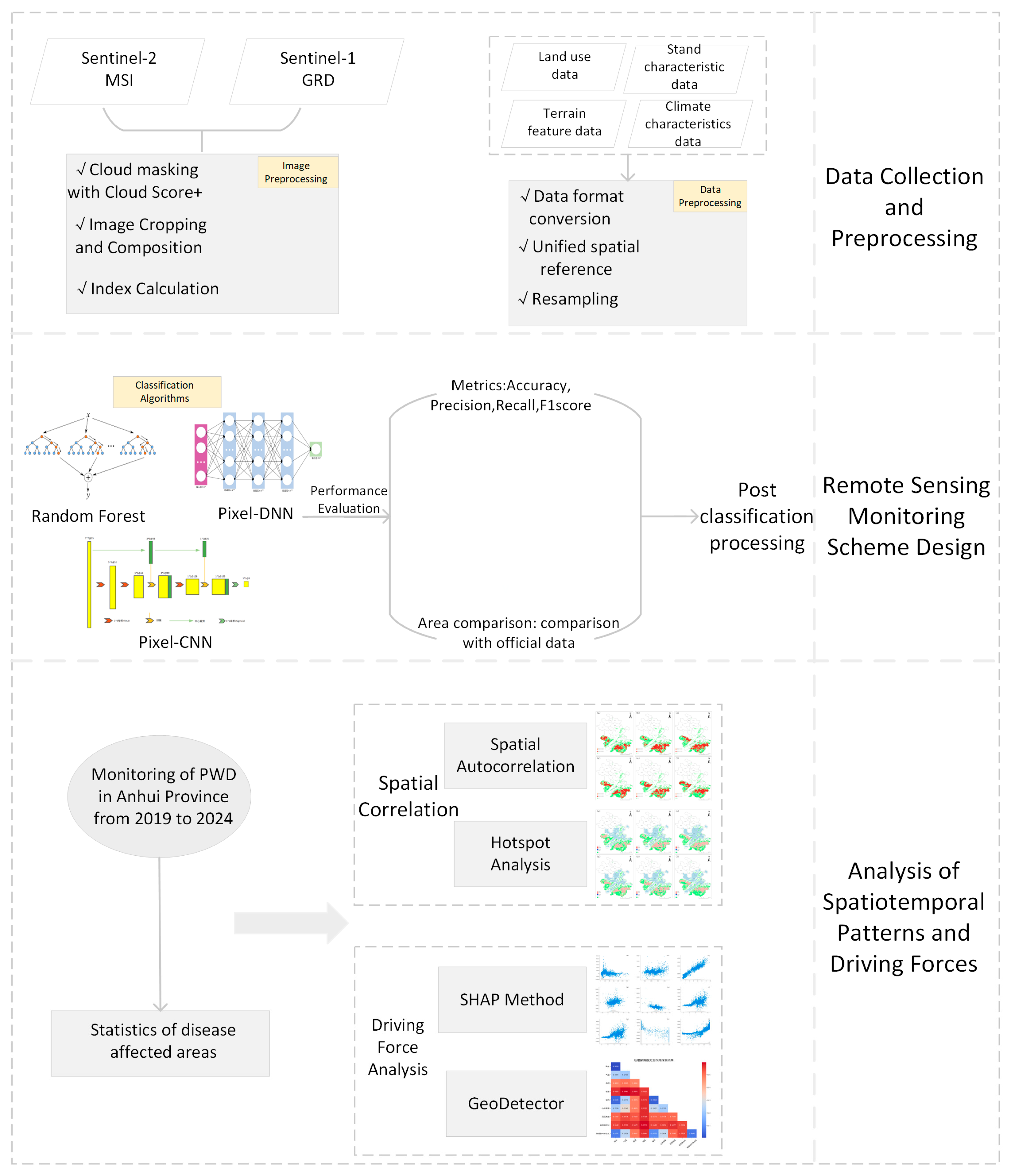
2. Materials and Methods

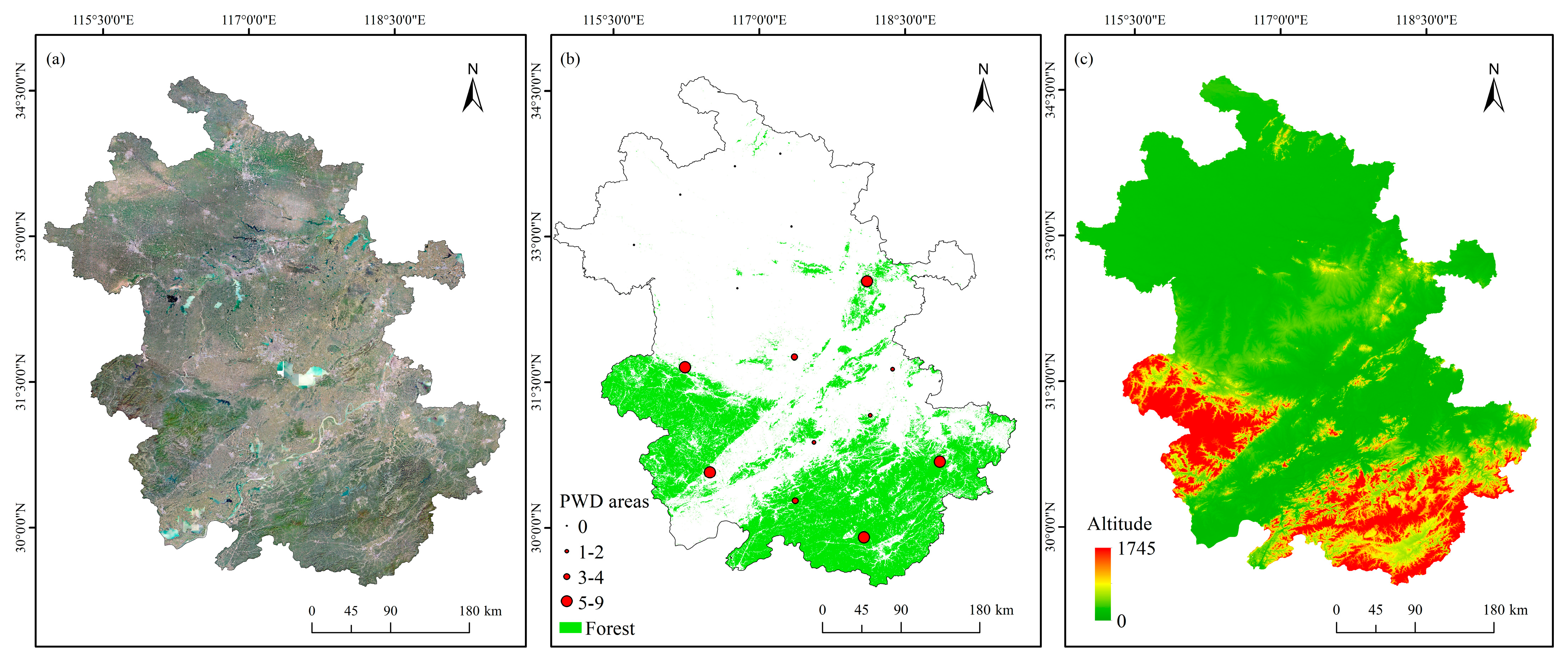
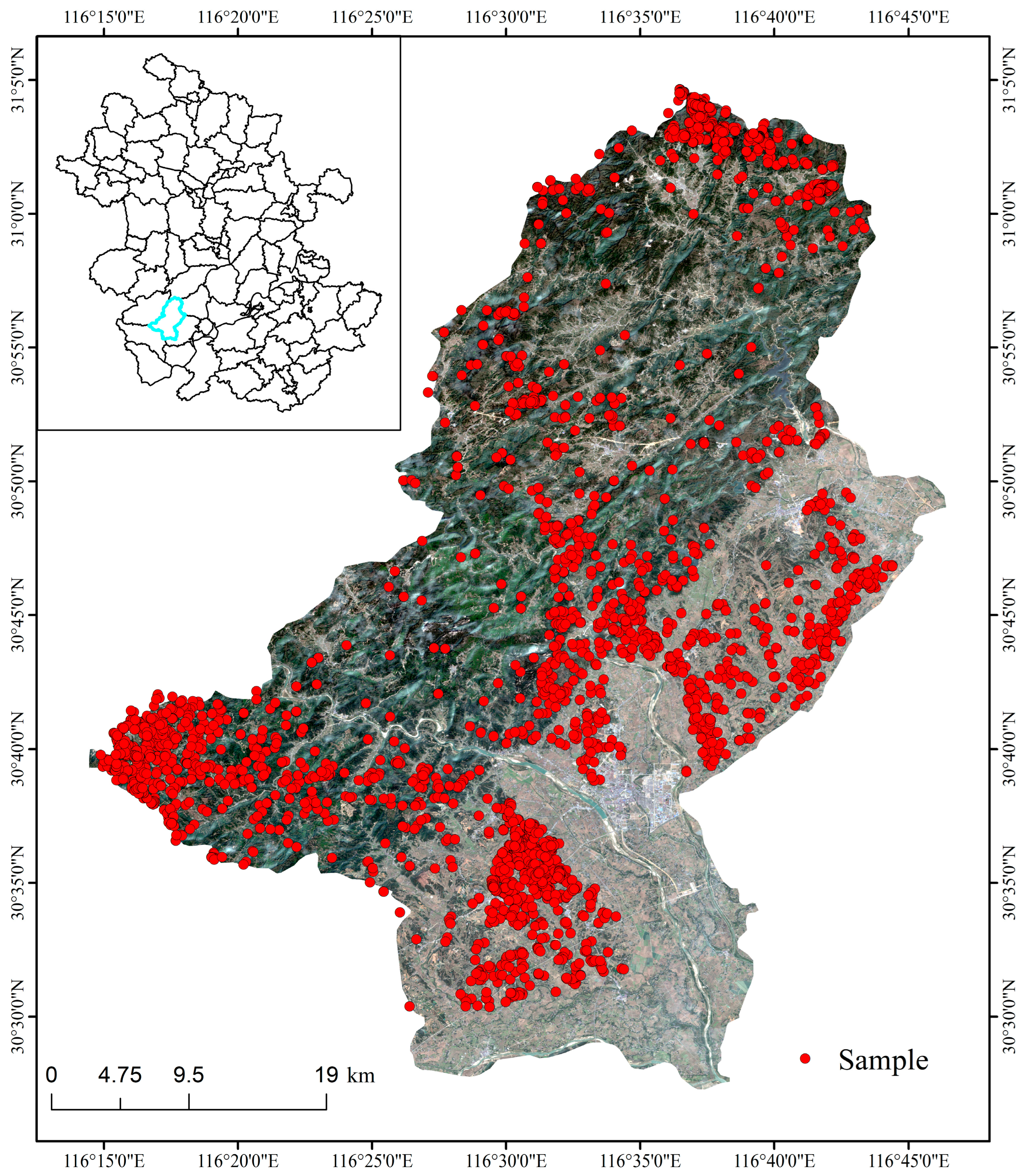
2.1. Study Area

Anhui Province, located in East China, comprises 16 prefecture-level administrative units as of December 2022. The province boasts abundant forest resources, with woodland areas covering nearly one-third of its total territory, primarily concentrated in the mountainous regions of southern Anhui and the Dabie Mountains [27]. During the 13th Five-Year Plan period, Anhui’s forest coverage rate reached 30.22%, with coniferous forests accounting for 27.29% of the total woodland area. Due to its rich forest resources, Anhui Province has long been affected by pine wilt disease. The province currently has 49 PWD epidemic zones, mainly distributed across southern Anhui region (Figure 2).

To meet the sample requirements for subsequent deep learning research, this study selected Qianshan City as a representative study area for PWD remote sensing monitoring. Qianshan City is situated in the southwestern part of Anhui Province, spanning 30°27′ to 31°04′ north latitude and 116°14′ to 116°46′ east longitude. Located on the southeastern foothills of the Dabie Mountains, the terrain exhibits a step-like distribution pattern, gradually descending from northwest to southeast. The region features diverse ecological types with a high forest coverage rate of 39%, characterized by contiguous woodland areas and relatively stable ecosystem structures. As one of the areas most severely affected by pine wilt disease in Anhui Province, Qianshan City has experienced repeated outbreaks over the years. During the autumn of 2021, field investigations yielded 3923 infected pine tree samples (Figure 3). Each sample contains detailed information including serial numbers, township locations, GPS coordinates, and field observation notes, providing high-quality data support for remote sensing model training and validation. The optimal model parameters obtained from this study area were subsequently applied to province-wide homologous remote sensing data to generate a spatial distribution map of PWD across the entire province.

2.2. Data Sources and Preprocessing

2.2.1. Remote Sensing Imagery Data and Sample Preparation

This study selects Sentinel-2A imagery as the primary data source for monitoring pine wilt disease, utilizing 12 spectral bands (B1 to B12) as the main input features [28]. The outbreak period of PWD predominantly occurs during autumn (September to November), representing the optimal monitoring window. To mitigate the impact of clouds and cloud shadows on image quality, we implemented a joint cloud removal approach combining Sentinel-2A’s QA band with the Cloud Score+ dataset. In accordance with the official recommendation, this study adopts a cloud threshold of 0.64 to facilitate effective cloud removal [29].

Sentinel-1 offers four imaging modes, three data product types, and four polarization modes. Based on a review of historical literature and the actual geographical characteristics of the study area [30], this study selects the interferometric wide swath (IW) mode as the imaging mode. For polarization, both VV (vertical–vertical) and VH (vertical–horizontal) polarization modes were chosen to fully utilize the sensitivity of different polarization information to surface features.

The first step involves unifying the coordinate reference systems between the sample data and image data before performing image overlay to create the infected tree sample set. To balance sample categories, this study selected some healthy tree samples to expand the sample set and prevent model overfitting. The sampleRegions() function was used to associate the spectral information of the images with the geographical locations of the sample points, generating training samples containing spectral features and category labels. The dataset was then split into training and validation sets at a 7:3 ratio. To support subsequent deep learning model training, tile samples were further prepared.

2.2.2. Influencing Factors

To investigate the relationship between precipitation and pine wilt disease distribution, this study selected precipitation and temperature data as driving factors [6]. We utilized China’s 1 km-resolution monthly precipitation dataset and monthly mean temperature dataset for September and October 2021 [26], with validation performed using data from 496 independent meteorological observation stations.

Tree characteristics included tree height, natural/plantation forest distribution, and woodland categories. Among these, the ETH Global Tree height Dataset was generated using multi-temporal Sentinel-2 multispectral imaging satellite data combined with deep learning methods and can be directly accessed and analyzed on GEE [31].

The Global Natural/Planted Forest Dataset (GNPFD) was developed using Landsat imagery from 1985 to 2021 as primary data sources. This dataset employed a random forest model integrated with multi-source auxiliary data to generate global distribution maps of planted and natural forests for 2021. Training samples were created through change detection algorithms analyzing disturbance frequency and time-series variations between 1985 and 2021, enabling the production of global forest-type maps spanning 1985–2020.

The MCD12Q1.061 dataset (https://lpdaac.usgs.gov/products/mcd12q1v061/, accessed on 6 June 2025) incorporates the Annual International Geosphere–Biosphere Programme (IGBP) classification scheme. This comprehensive system categorizes global land cover into 17 primary classes, with forest ecosystems further classified into evergreen needleleaf forests, evergreen broadleaf forests, deciduous needleleaf forests, deciduous broadleaf forests, and mixed forests. For topographic analysis, this study utilized the Shuttle Radar Topography Mission (SRTM) data, selected for its high precision (30 m resolution) and global coverage.

The ESRI Land Cover Dataset demonstrates an annual classification accuracy exceeding 75% for land use categories. This study utilized this dataset to extract annual forest cover extents across Anhui Province from 2019 to 2023, employing mask techniques to exclude monitoring values outside these designated forest areas. Furthermore, the Dynamic World dataset was incorporated to delineate Anhui Province’s 2024 forest coverage. Through integration with PWD monitoring results, this approach enabled the systematic elimination of detection outcomes falling outside forested boundaries, ensuring spatial accuracy in disease distribution mapping.

2.3. Methods

2.3.1. Feature Settings

• Training samples and validation samples production

First, unify the coordinate reference systems of the sample data and the image data by adopting the WGS84 geographic coordinate system to avoid spatial deviations caused by inconsistent coordinate systems. Then, overlay the sample points with high-resolution satellite imagery, and after removing scattered diseased tree samples, load the remaining samples along with Sentinel-2 satellite imagery into the same layer. A new diseased tree sample set is reconstructed based on the pixel centers where the diseased trees are located. To balance the sample categories, this study selected a portion of healthy tree samples to expand the sample set, ensuring category balance within the sample set and preventing the model from overfitting [32].

On the Google Earth Engine platform, the sampleRegions() function is used to extract the pixel values corresponding to the sample point locations and assign them to the sample points. This function spatially matches the spectral information from the image data with the geographic locations of the sample points, generating a training sample dataset that includes spectral features and class labels. Subsequently, the data is exported as a CSV file to serve as sample data for subsequent model training. The sample data is then split into training and validation sets in a 7:3 ratio.

To support the training of subsequent deep learning models, it is necessary to further produce sample patches. First, based on the latitude and longitude coordinates in the CSV file, the GDAL library is used to convert them into row and column numbers in the imagery. This step ensures the spatial consistency between sample points and image data by leveraging the mapping relationship between geographic coordinates and image coordinates. Next, a 7 × 7-pixel sample patch is cropped with the sample point as the center. This patch size provides sufficient local spatial information for the deep learning model, while avoiding redundant computation caused by excessively large patches. The cropped sample patches will serve as model inputs for training and validation. The category labels in the CSV file correspond to the class information of the sample patches. Subsequently, based on the geotransform, the row and column numbers of the patches are converted back into latitude and longitude coordinates, ultimately generating a sample patch dataset with spatial information. The generation of sample patches can provide local spatial context information for deep learning models such as convolutional neural networks.

2.

Original Feature Construction

This study constructs the feature set from two aspects—spectral features and radar features. In PWD monitoring, infection causes physiological changes in trees, leading to alterations in spectral reflectance curves [33]. These differences can be leveraged for PWD detection. Based on Sentinel-2 satellite bands, this study selects 10 m-resolution and 20 m-resolution bands for the original feature set to facilitate subsequent analysis.

For radar features, Sentinel-1 data was used as the primary source [34]. Due to Sentinel-1’s ascending and descending orbit configurations, initial filtering and statistical analysis were performed in GEE based on the study area. Since ascending orbit images dominated the dataset, this study exclusively used Sentinel-1 ascending orbit data as the radar source, with VV and VH polarizations selected as the key band features. In this study, the SAR variables correspond to the sigma naught (σ⁰) backscatter coefficients provided by Sentinel-1 in the VV and VH polarizations. As the original data is in decibel (dB) units in GEE, it was converted to linear power units prior to processing. To ensure consistent spatial resolution, the resample function is used in GEE to resample the spatial resolution of Sentinel-1 to match that of Sentinel-2, using the bilinear sampling method.

Due to the significant impact of extensive speckle noise in SAR images on both image quality and the accuracy of subsequent analyses, this study employs the refined Lee filter algorithm to denoise the Sentinel-1 images [35]. The refined Lee filter employs multiple moving window sizes to enhance speckle reduction, while preserving image details. Specifically, a 3 × 3 window is utilized for computing local statistics, such as mean and variance. A 7×7 sampling window is applied to estimate local noise and determine gradient directions, which guide the directional filtering process. Finally, a set of 7 × 7 directional windows (rectangular and diagonal) is employed to compute directionally adaptive mean and variance values, ensuring edge preservation and improved speckle suppression. This algorithm improves upon the traditional Lee Filter by introducing an edge detection mechanism, dynamically adjusting window sizes, and optimizing the noise model [35].

In the monitoring of pine wilt disease, remote sensing indices enhance the contrast between infected and healthy trees by combining different feature information to highlight distinguishing characteristics. Based on extensive prior research, a total of 38 features were selected for modeling in this study. These include 10 spectral bands from Sentinel-2 (B2–B8, B8A, B11, and B12), 2 radar backscatter coefficients from Sentinel-1 (VV and VH), and 26 optical remote sensing indices (

Table 1. The 26 optical remote sensing indices derived from Sentinel-2 images.

Index Name	Calculation Formula	Reference
GNDVI	${\displaystyle \frac{\mathrm{B}8-\mathrm{B}3}{\mathrm{B}8+\mathrm{B}3}}$	[36]
SAVI	${\displaystyle \frac{\left(\mathrm{B}8-\mathrm{B}4\right)\left(1+\mathrm{L}\right)}{\left(\mathrm{B}8+\mathrm{B}4+\mathrm{L}\right)}}$	[36]
RGI	${\displaystyle \frac{\mathrm{B}4}{\mathrm{B}3}}$	[36]
MSR2	${\displaystyle \frac{\left(\frac{\mathrm{B}8}{\mathrm{B}4}-1\right)}{\sqrt{\frac{\mathrm{B}8}{\mathrm{B}4}+1}}}$	[36]
NDVIgreen	${\displaystyle \frac{\mathrm{B}3-\mathrm{B}4}{\mathrm{B}3+\mathrm{B}4}}$	[37]
NDVInir	${\displaystyle \frac{\mathrm{B}8\mathrm{A}-\mathrm{B}4}{\mathrm{B}8\mathrm{A}+\mathrm{B}4}}$	[37]
NDVIswir	${\displaystyle \frac{\mathrm{B}8\mathrm{A}-\mathrm{B}11}{\mathrm{B}8\mathrm{A}+\mathrm{B}11}}$	[37]
REIP	$700+40\times {\displaystyle \frac{\left(\frac{\mathrm{B}4+\mathrm{B}7}{\mathrm{B}2}-\mathrm{B}5\right)}{\left(\mathrm{B}6-\mathrm{B}5\right)}}$	[37]
TCG	$0.2848\times \mathrm{B}2-0.2453\times \mathrm{B}3-0.5436\times \mathrm{B}4+0.7243\times \mathrm{B}8\mathrm{A}+0.0840\times \mathrm{B}11-0.18\times \mathrm{B}12$	[37]
TCW	$0.1509\times B2+0.1973\times \mathrm{B}3+0.3279\times \mathrm{B}4+0.3406\times \mathrm{B}8-0.7112\times \mathrm{B}11-0.4572\times \mathrm{B}12$	[37]
BWDRVI	${\displaystyle \frac{0.1\times \mathrm{B}8-\mathrm{B}2}{0.1\times \mathrm{B}8+\mathrm{B}2}}$	[38]
GLI	${\displaystyle \frac{2\times \mathrm{B}3-\mathrm{B}4-\mathrm{B}2}{2\times \mathrm{B}3+\mathrm{B}4+\mathrm{B}2}}$	[38]
NDVIre	${\displaystyle \frac{\mathrm{B}5-\mathrm{B}4}{\mathrm{B}5+\mathrm{B}4}}$	[38]
SLAVI	${\displaystyle \frac{\mathrm{B}8}{\mathrm{B}4+\mathrm{B}11}}$	[38]
NDMI	${\displaystyle \frac{\mathrm{B}8-\mathrm{B}11}{\mathrm{B}8+\mathrm{B}11}}$	[39]
NBR	${\displaystyle \frac{\mathrm{B}8-\mathrm{B}12}{\mathrm{B}8+\mathrm{B}12}}$	[39]
DSWI	${\displaystyle \frac{\mathrm{B}8+\mathrm{B}3}{\mathrm{B}11+\mathrm{B}4}}$	[40]
RDVI	${\displaystyle \frac{\mathrm{B}8-\mathrm{B}4}{\sqrt{\mathrm{B}8+\mathrm{B}4}}}$	[40]
Ndre1	${\displaystyle \frac{\mathrm{B}8\mathrm{A}-\mathrm{B}5}{\mathrm{B}8\mathrm{A}+\mathrm{B}5}}$	[3]
Ndre2	${\displaystyle \frac{\mathrm{B}8\mathrm{A}-\mathrm{B}6}{\mathrm{B}8\mathrm{A}+\mathrm{B}6}}$	[3]
Ndre3	${\displaystyle \frac{\mathrm{B}8\mathrm{A}-\mathrm{B}7}{\mathrm{B}8\mathrm{A}+\mathrm{B}7}}$	[3]
RVSI	${\displaystyle \frac{\mathrm{B}5+\mathrm{B}7}{2}}-\mathrm{B}6$	[3]
GARI	${\displaystyle \frac{\mathrm{B}8-\left(\mathrm{B}3-1.7\times \left(\mathrm{B}2-\mathrm{B}4\right)\right)}{\mathrm{B}8+\left(\mathrm{B}3-1.7\times \left(\mathrm{B}2-\mathrm{B}4\right)\right)}}$	[38]
ARI	${\displaystyle \frac{1}{\mathrm{B}3}}-{\displaystyle \frac{1}{\mathrm{B}5}}$	[3]
PBI	${\displaystyle \frac{\mathrm{B}8\mathrm{A}}{\mathrm{B}3}}$	[3]
MNDWI	${\displaystyle \frac{\left(\mathrm{B}3-\mathrm{B}11\right)}{\left(\mathrm{B}3+\mathrm{B}11\right)}}$	[40]

).

3.

The Recursive Feature Elimination

The recursive feature elimination (RFE) algorithm is a feature selection method that recursively removes the least important features to identify the optimal feature subset [41]. To reduce feature redundancy and accelerate model training, this study employed recursive feature elimination (RFE) to decrease the number of features. The results showed that the number of features was reduced from 38 to 25, eliminating a total of 13 features. The final features used for modeling were B2, B3, B4, B5, B6, B8, B8A, B12, NDVIgreen, SAVI, RVSI, NDVIre1, TCG, TCW, BWDRVI, GLI, NDMI, GNDVI, RGI, REIP, SLAVI, NBR, DSWI, GARI, and PBI.

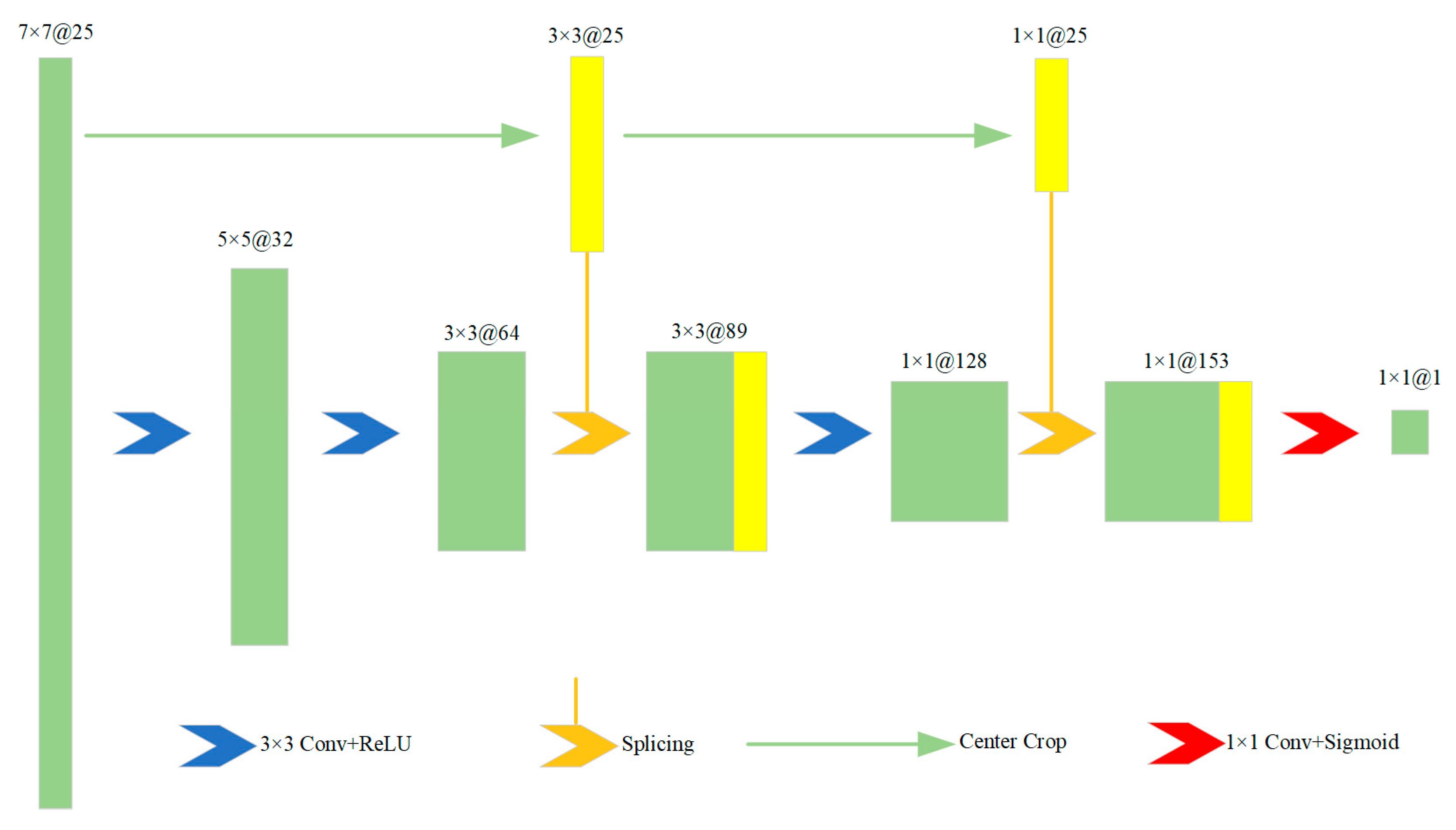
2.3.2. Monitoring Models

1.

Convolutional Neural Network Model

Convolutional neural networks (CNN), as regularized feedforward neural networks with strong representational capabilities in deep learning, demonstrate remarkable advantages in image feature learning and pattern recognition through their unique local connectivity and weight-sharing mechanisms [42]. This network architecture achieves hierarchical abstraction from low-level visual features to high-level semantic features through cascaded feature extraction modules. Its typical structure consists of an input layer, convolutional layers, pooling layers, and fully connected layers, forming a modular processing pipeline where nonlinear transformations and parameter optimization between layers establish an end-to-end feature learning system.

In this study, a pixel-based CNN model (Figure 4) was constructed using the PyTorch (version 2.0.0)deep learning framework [43] with CUDA 11.8 support. The model takes a 7 × 7@25 image patch as input (where 25 denotes the number of features). After two rounds of 3 × 3 convolution, the feature map size reduces to 3 × 3@64. This output is then concatenated with the central 3 × 3 region of the input image, resulting in a 3 × 3@89 feature map. Subsequent convolution and concatenation operations further transform the dimensions to 1 × 1@153. Finally, a 1 × 1 convolution and Sigmoid activation function are applied to determine the class probability of the central pixel. The loss is computed based on the label value and predicted probability. During training, the batch size was set to 64 with 150 iterations. Adam was ultimately selected as the optimizer with a learning rate of 1e-3. The loss function used is BCELoss. An early stopping mechanism is employed; if the validation loss does not decrease for more than 15 consecutive epochs, the training will be stopped.

2.

Deep Neural Network Model

Deep neural network (DNN) is a feedforward neural network featuring multiple layers of nonlinear transformations [44].

The core concept of DNN lies in its hierarchical abstraction of data features, enabling the automatic learning of complex patterns from raw data. Capable of extracting deep feature representations from vast amounts of unlabeled data, DNN demonstrates exceptional performance in processing image, audio, and text data. In this study, a pixel-based DNN model (Figure 5) was implemented using the PyTorch (version 2.0.0) deep learning framework [43] with CUDA 11.8 support. The model architecture consists of one input layer with 25 neurons, three hidden layers with 128, 256, and 512 neurons, respectively, and one output layer with 1 neuron. The training parameter configuration remains consistent with that of the pixel-based CNN model.

3.

Random Forest Model

Random forest (RF) is an ensemble learning method that enhances model accuracy and controls overfitting by constructing multiple decision trees and combining their predictions [45,46]. During training, the algorithm generates numerous decision trees, with each tree trained on a bootstrap sample (sampling with replacement) from the original dataset. At each node, only a randomly selected subset of features is considered for splitting. The final prediction is determined through majority voting across all trees. As a result, the random forest model exhibits strong generalization capability, suitability for high-dimensional data, high accuracy, and robust performance. Due to these advantages, it is widely applied to both classification and regression problems [47]. On the Google Earth Engine (https://earthengine.google.com/, accessed on 6 June 2025 ) platform, the ee.Classifier.smileRandomForest() function is used to build a random forest model. The optimal classifier is obtained by dynamically adjusting the following two key parameters: numberOfTrees and minLeafPopulation [48]. The former represents the number of decision trees to be created, while the latter controls the minimum number of samples required at each leaf node, thereby influencing the model’s complexity and degree of fitting. Based on the results of multiple experiments, this paper sets the numberOfTrees to 300 and the minLeafPopulation to 3.

4.

Accuracy Metrics Evaluation and Classification Processing

To evaluate model performance quantitatively, this study adopts four accuracy metrics—accuracy, precision, recall, and F1-score [49,50]—computed as follows:

$$Accuracy={\displaystyle \frac{TP+TN}{TP+TN+FP+FN}}$$

(1)

$$Precision={\displaystyle \frac{TP}{TP+FP}}$$

(2)

$$\mathrm{Re}call={\displaystyle \frac{TP}{TP+FN}}$$

(3)

$$F1-score={\displaystyle \frac{2\times Precision\times \mathrm{Re}call}{Precision+\mathrm{Re}call}}$$

(4)

In the above formulas, TP (true positive) represents cases where the model predicts “true”, and the label value is also “true”; FP (false positive) represents cases where the model predicts “true”, but the label value is “false”; FN (false negative) represents cases where the model predicts “false”, but the label value is “true”; and TN (true negative) represents cases where the model predicts “false”, and the label value is also “false”. In this study, “true” refers to pine trees infected with pine wilt disease, while “false” refers to non-infected pine trees.

To further optimize the accuracy of identifying pine wilt disease-infected trees, this study extracted forest land data from land use data as a mask. The classification results were then masked and extracted using the forest land data, removing parts of the classification results that did not belong to forested areas, thereby ensuring the accuracy of the classification results. To validate the model’s performance at the provincial scale, this study collected data on pine wilt disease epidemic areas in Anhui Province from 2019 to 2021, provided by the forestry department of Anhui Province, and compared them with the monitoring results of this study to verify the performance of the algorithm used.

2.3.3. Spatiotemporal Pattern Analysis

1.

Spatial autocorrelation analysis

Spatial autocorrelation analysis is commonly used to assess the correlation between spatial data, measuring whether data values distributed across different geographic locations are interrelated [51,52]. In this study, Moran’s I index was employed to evaluate the spatial patterns and characteristics of pine wilt disease distribution in Anhui Province.

Moran’s I index is further divided into global Moran’s I and local Moran’s I. The formula for calculating the global Moran’s I index is as follows:

$$I={\displaystyle \frac{n{\displaystyle \sum _{i=1}^n{\displaystyle \sum _{j=1}^n{w}_{ij}\left(y_i-\overline{y}\right)\left(y_j-\overline{y}\right)}}}{\left({\displaystyle \sum _{i=1}^n{\displaystyle \sum _{j=1}^n{w}_{ij}}}\right){\displaystyle \sum _{i=1}^n{\left(y_i-\overline{y}\right)}^2}}}$$

(5)

where n is the number of spatial data, $y_i$ and $y_j$ are the attribute values of the object at points i and j, $\overline{y}$ is the average value of $y_i$ and $y_j$, and the spatial weight matrix $w_{ij}$ represents the connection relationship between the spatial objects at point i and j. If the data values of adjacent locations tend to be similar, there is a positive spatial autocorrelation. If the data values of adjacent locations tend to be different, there is a negative spatial autocorrelation. If there is no obvious pattern, then the data may be randomly distributed.

This study employs the global Moran’s I to analyze spatial clustering characteristics and local Moran’s I to measure spatial correlations among observed values.

2.

High/Low Clustering and Hot Spot Analysis

High/low clustering analysis is a statistical method used to identify whether spatial data exhibits clustering of high or low values [53]. It reveals whether high or low values in a given spatial distribution are more likely to cluster together than would be expected under random conditions. Since high/low clustering is an inferential statistical method, the results are interpreted under the null hypothesis. If the p-value is sufficiently small and statistically significant, the null hypothesis can be rejected. Upon rejecting the null hypothesis, a positive z-score indicates that the spatial data exhibits clustering of high values across the study area, while a negative z-score suggests clustering of low values.

Hot spot analysis is a statistical method used to identify significant spatial clusters of high values (hot spots) or low values (cold spots) in geospatial data [54]. By evaluating the relationship between each location and its neighboring areas, it determines which regions exhibit statistically significant hot spots or cold spots. Hot spot analysis focuses more on identifying specific hot and cold spots and assessing their statistical significance; whereas, high/low clustering is better suited for describing the overall trend of high or low value aggregation across the entire study area. In this study, the high/low clustering and hot spot analysis tools in ArcGIS Pro were used to conduct high/low clustering and hot spot analyses for pine wilt disease in Anhui Province.

2.3.4. Driving Factor Analysis

1.

SHAP contribution analysis

SHAP is a method used to interpret the predictions of machine learning models [55]. Based on the concept of Shapley values from game theory, it provides a way to measure the contribution of each feature to individual predictions, offering precise feature importance scores and revealing interactions between features.

This study employs the SHAP method to assess the influence of various factors on pine wilt disease. First, a 5 km × 5 km fishing net grid was generated within the study area, and the statistical values of influencing factors and the infected area within each grid cell were calculated. Next, the statistical values of the influencing factors were used as independent variables, and the infected area as the dependent variable to construct a random forest regression model. Then, the Python SHAP library (version 0.41.0) was utilized to compute the SHAP values for each feature. SHAP values reflect the contribution of each feature to the model’s predictions—positive values indicate a positive influence on the prediction outcome, while negative values signify a negative influence.

2.

Geodetector

The Geodetector is a spatial statistical method used to analyze spatial differentiation and identify influencing factors, primarily employed to explore the spatial heterogeneity of geographical phenomena and determine which factors significantly contribute to such heterogeneity [56]. The Geodetector has the following four main functions: differentiation detection, factor detection, risk detection, and interaction detection. The factor detector assesses the influence of each factor on the non-grain conversion of cropland, represented by the q-value. A higher q-value indicates a stronger explanatory power of the factor on the incidence area of pine wilt disease, while a lower value suggests a weaker explanatory power. The p-value is used to determine whether the explanatory power is statistically significant.

This study utilized the Geodetector to analyze the main influencing factors and interaction characteristics of pine wilt disease in Anhui Province in 2021. Climate-related factors included precipitation and temperature (2 factors), tree characteristics included natural forest area, tree height, and evergreen coniferous forest area (3 factors), and topographic features included elevation, slope, and aspect (3 factors). These nine influencing factors were treated as independent variables Xi (I = 1, 2, 3, …, 9), with the affected area of pine wilt disease as the dependent variable Y, to analyze the main influencing factors and interaction characteristics of pine wilt disease in Anhui Province in 2021. To ensure the proper operation of the Geodetector, the influencing factor data was first classified into six categories using the natural breaks method. A 5 km × 5 km fishing net was created in ArcGIS, and after removing outliers, the Geodetector was applied to perform differentiation detection, factor detection, and interaction detection.

3. Results and Discussion

3.1. Model Performance of Different Remote Sensing Monitoring Models

The experimental results (

Table 2. Model performance of different models.

Model	Accuracy	Precision	Recall	F1-Score
Pixel-DNN	0.691	0.656	0.720	0.686
Pixel-CNN	0.743	0.733	0.759	0.746
RF	0.789	0.779	0.805	0.791

) show that among the three models, the random forest model performs the best, with accuracy, precision, recall, and F1-score of 0.789, 0.778, 0.805, and 0.791, respectively. The CNN model comes next, achieving accuracy, precision, recall, and F1-score of 0.743, 0.733, 0.759, and 0.746, respectively. The DNN model performs the worst, with accuracy, precision, recall, and F1-score of 0.691, 0.656, 0.720, and 0.686, respectively.

The experimental results (Table 2) indicate that the CNN model did not outperform traditional machine learning models, which may be attributed to the small sample dataset, limited information from surrounding pixels, and the relatively simple structure of the deep learning model.

Although this study collected over 3900 field samples of diseased trees, many of them were isolated individual trees. In the remote sensing images, the pixels corresponding to these individual trees predominantly exhibited characteristics of healthy trees rather than infected ones, necessitating their exclusion from subsequent training. Additionally, due to the 10 m resolution limitation of Sentinel-2 imagery, a single pixel often contained multiple diseased tree samples, further reducing the effective sample size. As a result, the final training dataset in this study comprised only 623 samples. Deep learning models typically require large-scale training datasets to uncover underlying patterns in the data; whereas, machine learning models are less demanding in terms of sample size. This explains why the random forest model in this study outperformed both the CNN and DNN models.

The CNN model primarily relies on operations such as convolution and pooling to fully utilize the feature information of surrounding pixels for image classification. In this study, the CNN model used the features of seven neighboring pixels to determine the class of the central pixel. However, due to the low spatial resolution of the imagery employed, some sample patches contained fewer pixels representing pine wilt disease compared to those representing healthy trees. This imbalance hindered the model’s ability to learn relevant features from the data, thereby reducing its performance. In contrast, machine learning models classify based on individual pixels and do not need to account for surrounding pixel information. As a result, they avoid interference from healthy tree pixels, which in turn enhances their classification performance.

The deep learning models used in this study adopted a relatively simple architecture with insufficient complexity, making them prone to overfitting during training—performing well on the training set but poorly on the test set. In contrast, the random forest model mitigates overfitting risks by integrating multiple decision trees, thereby exhibiting stronger generalization capability. Considering these factors collectively, the random forest model outperformed both the CNN and DNN models in this study.

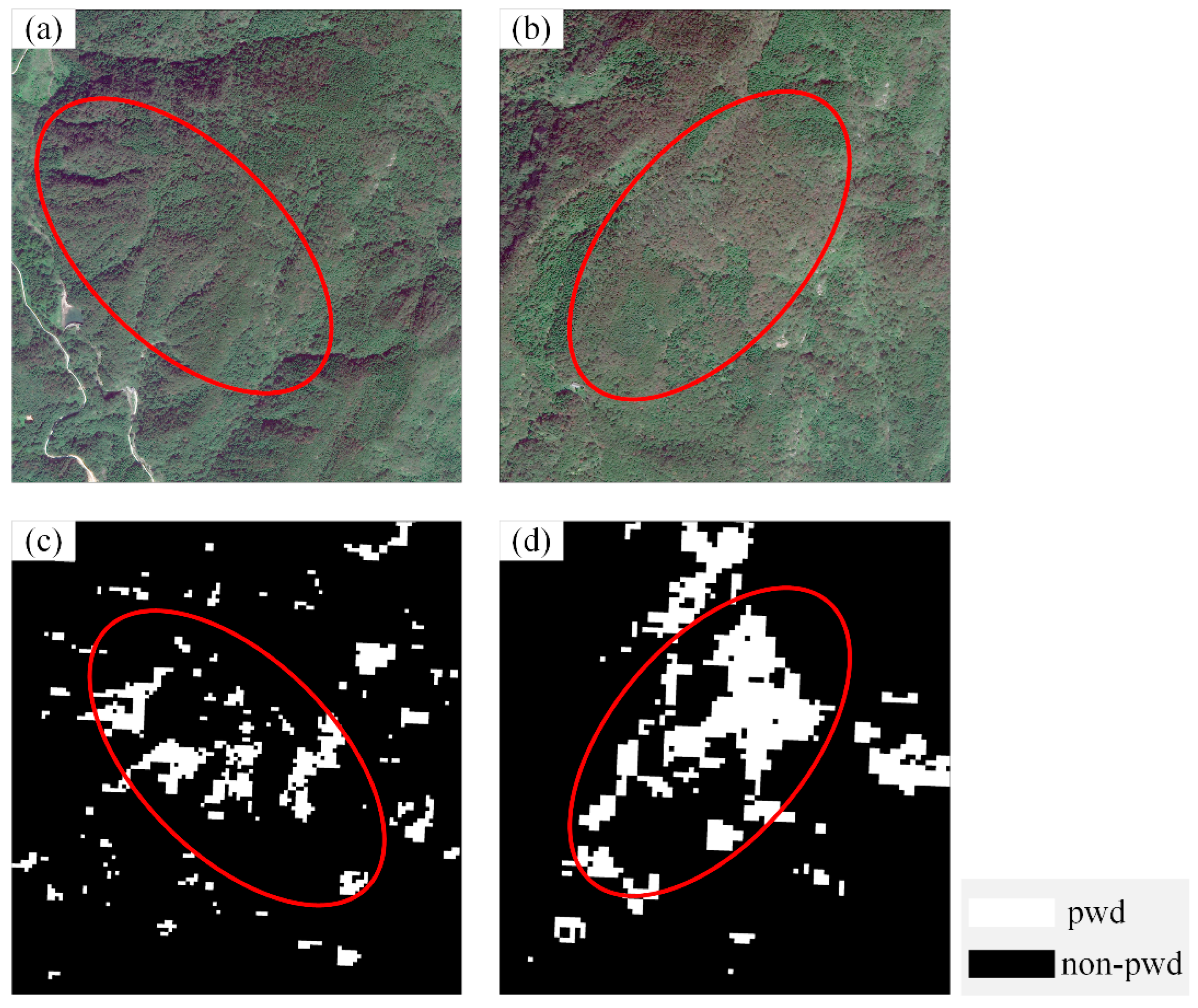
3.2. Accuracy Validation of the Optimal Classification Model

Based on the random forest model, this study calculated the annual infected area of pine wilt disease from 2019 to 2024 (Figure 6) and compared the results with official statistical data from 2019 to 2021 (

Table 3. Comparison of monitored areas of PWD from 2019 to 2021 (ha).

Year	Statistical Area	Monitored Area	Monitoring Error
2019	110,000	137,765	25.24%
2020	101,333	124,358	22.72%
2021	92,700	115,273	24.35%

). The monitoring area errors were 25.24%, 22.72%, and 24.35%, respectively—all within an acceptable 30% margin—indicating that the monitoring results can serve as a reliable basis for subsequent analysis.

The primary reason for the larger monitored area compared to official statistics lies in different methodological approaches. This study used 10 m resolution pixels as basic statistical units. During the research process, if any infected trees were present within a pixel, the entire pixel was classified as infected. Moreover, the spatial distribution of pine wilt disease often shows heterogeneity, with some areas containing sporadically distributed infected trees—a pattern that tends to be magnified in pixel-level statistics. While this approach provides more comprehensive spatial representation of disease distribution, it inevitably leads to overestimation compared to actual infected areas. In contrast, official statistics likely employed more precise field survey methods or different statistical criteria, resulting in relatively smaller infected areas. The observed errors (Table 3) remain within acceptable limits for 10 m resolution imagery data.

Based on the overall spatial distribution characteristics of pine wilt disease in the study area, this research selected monitoring results from two typical outbreak zones in Qianshan City for a visualization comparison with high-resolution imagery (Figure 7). As shown in the figure below, the monitoring method demonstrates significant advantages in identifying large-scale, contiguous infected pine trees. This is because such extensive infected areas exhibit distinct spectral feature changes in satellite imagery, enabling effective detection.

However, the study also revealed certain limitations in detecting small-scale, individual infected trees. This primarily occurs because single infected trees have relatively small canopies, and their characteristic features are often obscured by the shading effect of surrounding healthy trees, making it difficult to form noticeable spectral differences in medium-resolution satellite imagery. Additionally, the model tends to confuse mountainous shadow areas with infected zones. This misclassification arises because shadow regions present similar spectral and texture features to those of contiguous infected trees, making them difficult to distinguish. To address this issue, land use products were employed to extract corresponding annual forest coverage, and mask technology was applied to exclude non-forest areas from monitoring results. The ESRI Land Cover product was used for 2019–2023, while the Dynamic World product was adopted for 2024, ensuring the accuracy of identification results.

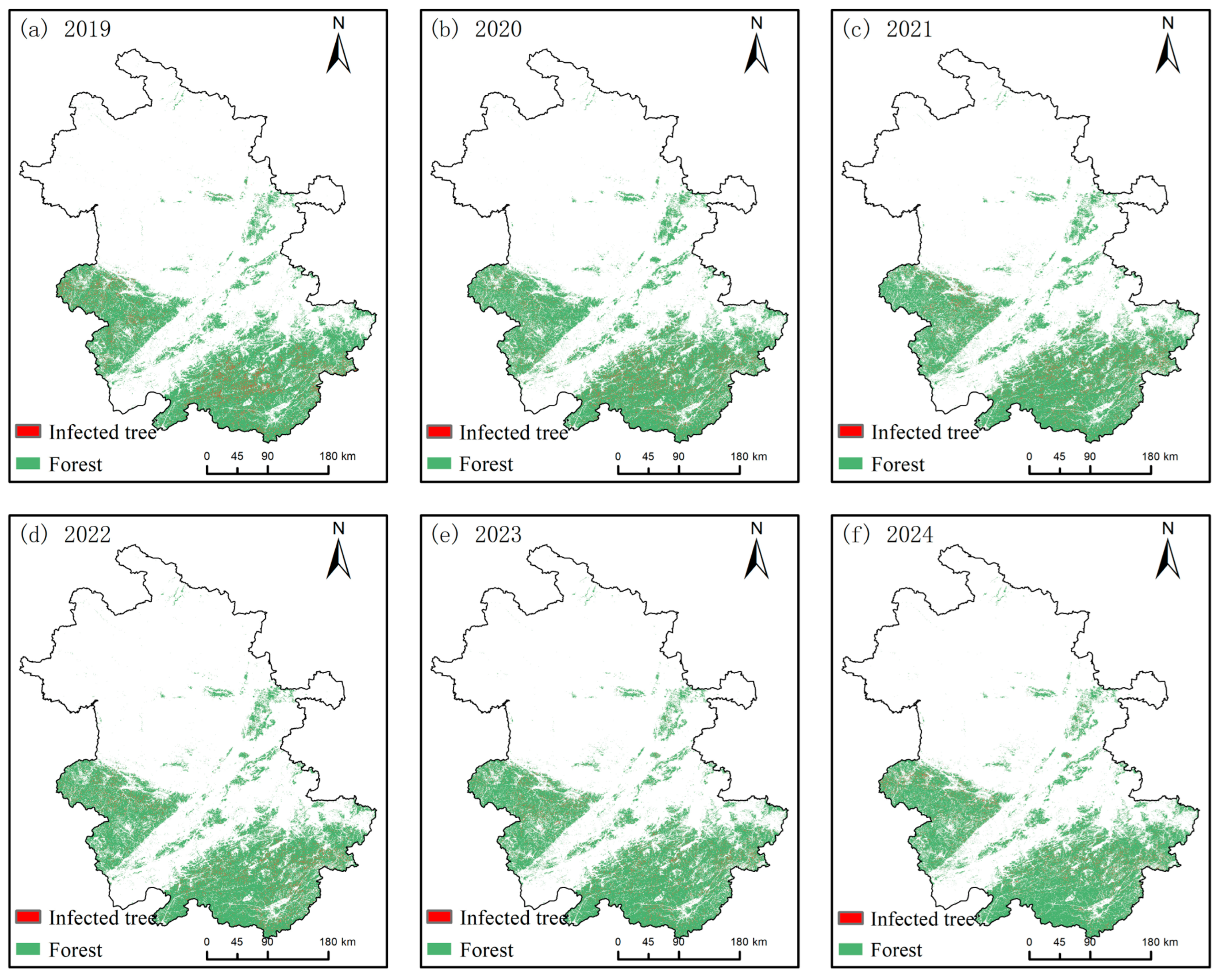
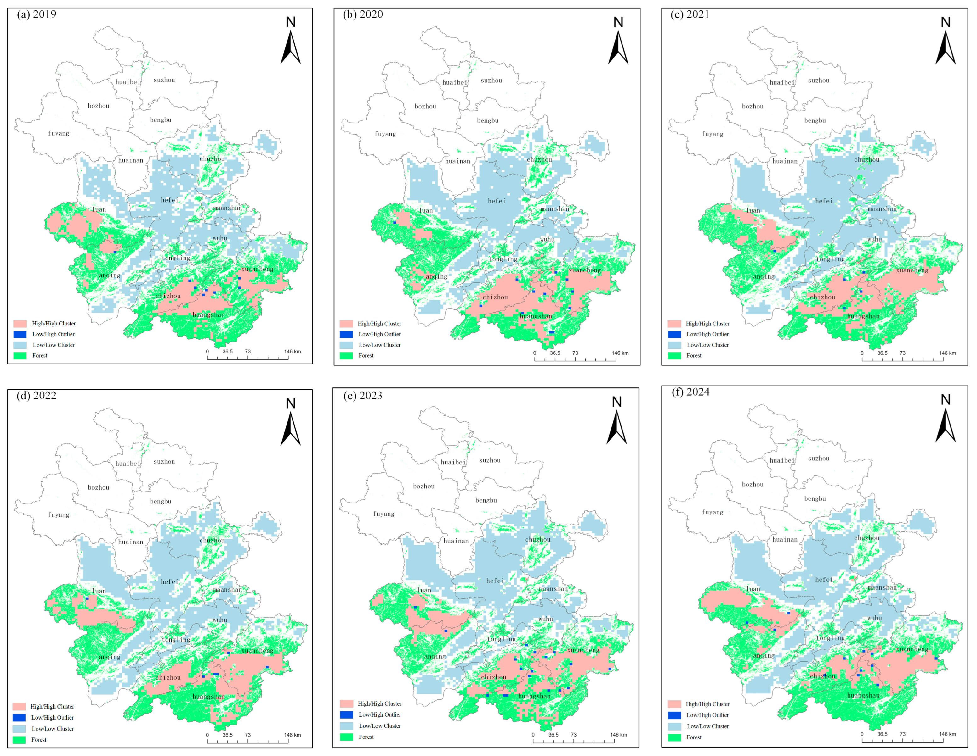
3.3. Spatiotemporal Dynamics of Pine Wilt Disease in Anhui Province

Analysis of pine wilt disease incidence statistics in Anhui Province from 2019 to 2024 reveals a consistent annual decline in affected areas. The infected area decreased from 137,765 hectares in 2019 to 88,443 hectares in 2024, representing a total reduction of 49,322 hectares (35.80%). The most significant single-year reduction occurred in 2020, with a decrease of 13,407 hectares. This sustained reduction in disease prevalence is closely associated with the province’s implementation of scientific prevention and control strategies since 2017. The comprehensive adoption of the Forest Chief System, coupled with precise and systematic management measures, has effectively curbed the spread of pine wilt disease.

The annual global Moran’s I index values (

Table 4. Global Molan index of pine wood nematode disease in Anhui Province from 2019 to 2024.

Year	Global Moran’s I	Z-Score	p-Value
2019	0.798	75.279	0
2020	0.850	80.113	0
2021	0.820	77.198	0
2022	0.840	79.212	0
2023	0.807	76.077	0

) demonstrate consistently high spatial autocorrelation, with all years except 2019 exceeding 0.8. These results indicate strongly positive spatial dependence in disease distribution, where adjacent or proximate areas exhibit similar infection probabilities, reflecting a highly clustered pattern. The peak value of 0.850 in 2020 particularly underscores the pronounced spatial dependency in the transmission trends and distribution characteristics of pine wilt disease.

At the 95% significance level, the LISA cluster maps of pine wilt disease occurrence areas from 2019 to 2024 (Figure 8) are presented as follows. In 2019, the spatial distribution of pine wilt disease in Anhui Province was primarily characterized by “High–High” and “Low–Low” clustering patterns. The “High–High” clusters were predominantly located in western and southern regions of the province, while the “Low–Low” clusters were mainly distributed in central and eastern areas, which generally exhibited milder epidemic conditions and might represent potential zones for disease spread. By 2020, a noticeable spatial transition was observed, with decreasing “High–High” clusters in western Anhui and increasing clusters in southern regions. This spatial shift suggests a potential disease migration from western to southern areas, likely attributable to several factors including climatic conditions, the distribution of pine forest resources, and regional variations in control measures. The humid climate and abundant pine resources in southern Anhui may have created favorable conditions for disease transmission. During 2021–2023, the “High–High” clusters showed a gradual northward shifting trend. In 2024, these high-incidence clusters became primarily concentrated in the following three cities: Lu’an, Xuancheng, and Chizhou. This spatial evolution may be associated with both the progressive implementation of control measures and natural disease diffusion patterns. As disease prevention efforts intensified in western and southern regions, the pathogen likely expanded into comparatively less protected northern areas. Furthermore, the distribution of pine resources and climatic conditions in northern regions may have provided new suitable environments for disease propagation.

Analysis of the high–low clustering results for pine wilt disease in Anhui Province from 2019 to 2024 (

Table 5. High–low clustering results of pine wood nematode disease in Anhui Province from 2019 to 2021.

Year	Observed Value	Expected Value	Z-Score	p-Value	Clustering Pattern
2019	0.000863	0.0002	75.091	0	High Clustering
2020	0.000659	0.0002	79.752	0	High Clustering
2021	0.000682	0.0002	76.902	0	High Clustering
2022	0.000711	0.0002	78.896	0	High Clustering
2023	0.000589	0.0002	75.755	0	High Clustering
2024	0.000667	0.0002	76.951	0	High Clustering

) reveals that the spatial distribution of the disease exhibited a statistically significant high-clustering pattern across all study years.

The local hotspot analysis results (Figure 9) reveal significant spatial–temporal variations in the distribution of pine wilt disease from 2019 to 2024. During 2019–2022, high-value clusters of pine wilt disease were primarily concentrated in western and southeastern regions of Anhui Province. However, in 2023 and 2024, sporadic disease outbreaks emerged in central areas, including Hefei and Chuzhou cities. This spatial pattern shift indicates an ongoing expansion of pine wilt disease from its traditional endemic zones in western/southeastern regions towards central parts of the province.

According to the analysis results of LISA agglomeration map in 2024 (Figure 8), the “high–high” spatial clustering of pine wood nematode disease in Anhui Province is mainly concentrated in the following three cities: Lu’an, Xuancheng and Chizhou. These areas have long been areas with high incidence of pine wood nematode disease, which may be related to the abundant pine forest resources, suitable climatic conditions for disease transmission, and historical epidemic accumulation. However, it is worth noting that in the central part of Anhui Province, especially in Hefei and Chuzhou, there is also a “high–high” spatial clustering phenomenon. This confirmed that the spatial distribution of pine wood nematode disease in Anhui Province was changing significantly, from a single-point concentrated outbreak trend to a multi-point diffusion outbreak trend.

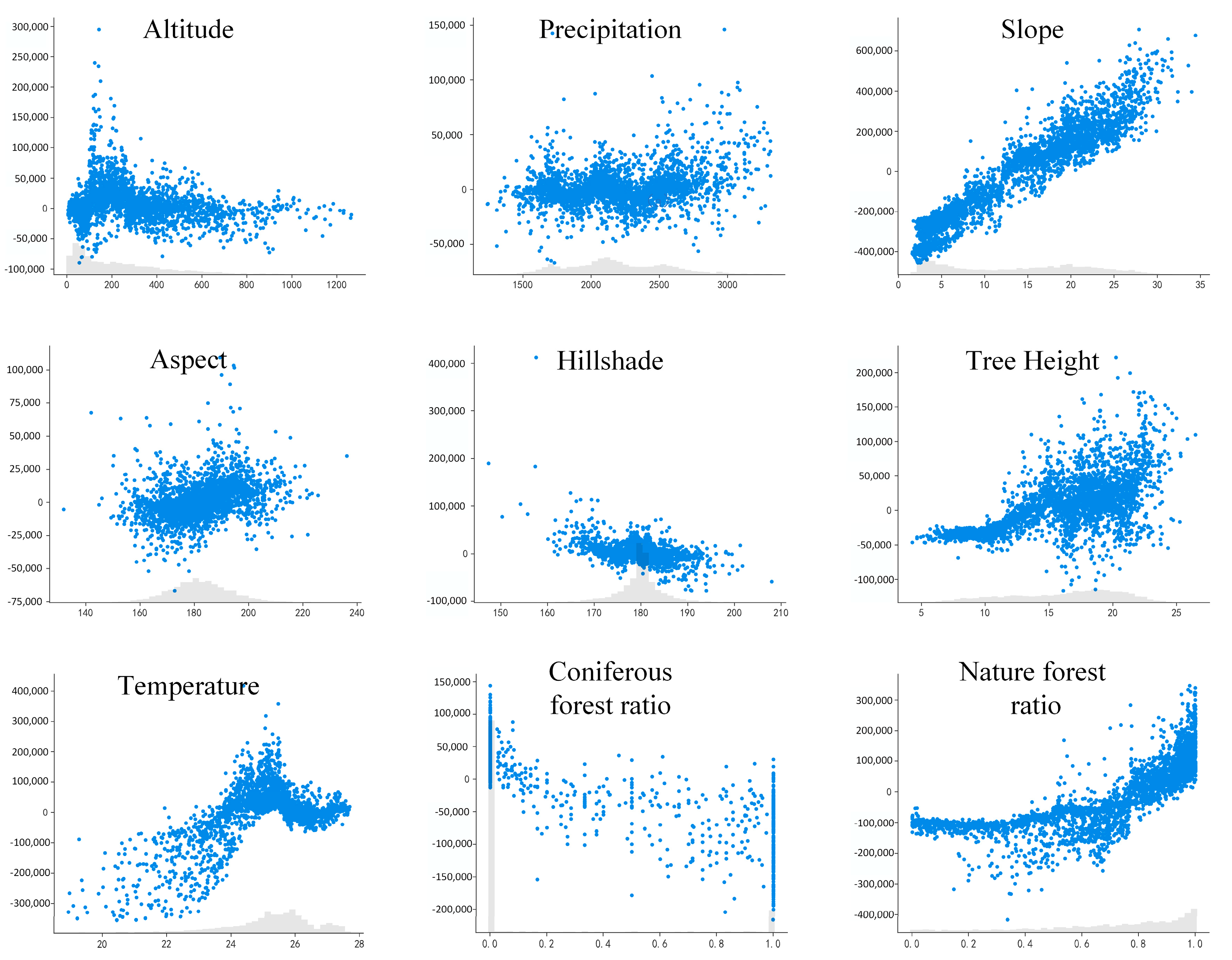
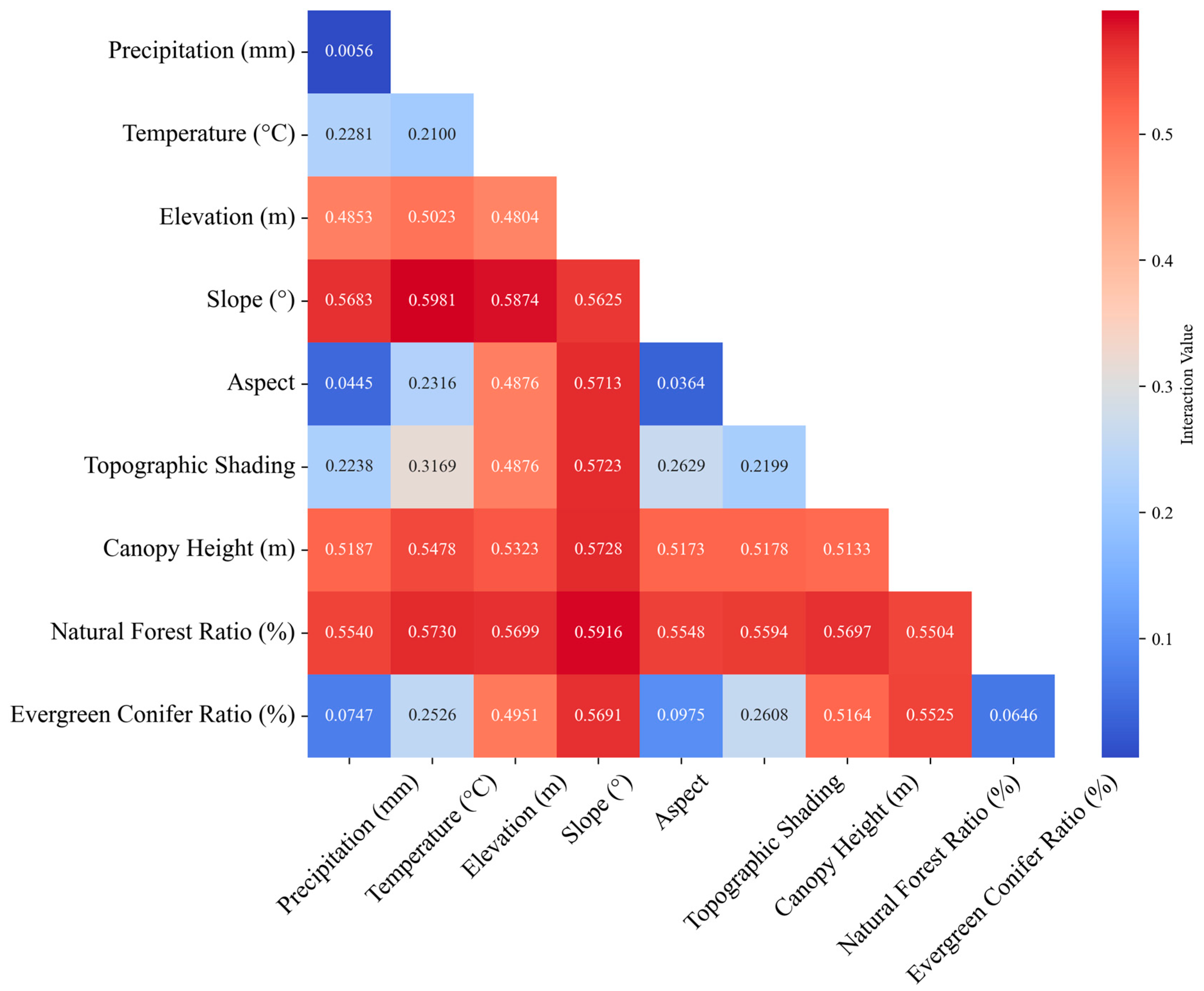
3.4. Driving Factors Analysis of Pine Wilt Disease in Anhui Province

According to the contribution degree of SHAP, the three largest contributories to the distribution of pine wood nematode disease were slope, natural forest percentage, and temperature, and the three smallest were precipitation, mountain shade, and slope aspect. Among them, the larger the slope, the greater the SHAP value, which indicates that the slope has a positive contribution to the distribution of pine wood nematode disease. From the perspective of the proportion of natural forests, the higher the proportion of natural forests, the greater the positive contribution to pine wood nematodes, which indicated that the ability of natural forests to resist pine wood nematode disease was weaker than that of plantations. Plantations, on the other hand, usually have a single tree species and dense pine trees, which have a low risk of initial infection despite the rapid transmission rate. The temperature factor is that when the temperature is moderate, the positive contribution value to the pine wood nematode is larger, because the pine wood nematode is active frequently at moderate temperature, the reproduction and development speed is accelerated, and it is easier to spread and spread in the host, resulting in the rapid spread of the disease.

According to the scatter plot results (Figure 10), the SHAP of temperature on pine wood nematode disease experienced a process of first rising and then decreasing, reaching the peak value of SHAP value at about 25°, and the lowest contribution to pine wood nematode disease at about 20° was negative, so it can be considered that 20° can effectively inhibit the occurrence of pine wood nematode disease, and 25 degrees is the best suitable temperature for pine wood nematode disease. There was a small peak at about 20–25 m in tree height, which indicated that there was a certain relationship between tree height and the occurrence of pine wood nematode disease. However, the percentage of natural forest showed a continuous upward trend; that is, the larger the proportion of natural forest, the higher the positive contribution to pine wood nematode disease.

In this study, Geodetector was used to analyze the distribution area of pine wood nematode disease in Anhui Province, and nine influencing factors in three aspects were used to analyze the influence. The experimental results show that the explanatory power of the slope factor and the temperature factor is the highest, which is 0.5981. These results indicated that climatic factors and natural conditions had the most significant impact on the distribution of pine wood nematode disease in Anhui Province.

According to the results (Figure 11), the explanatory power of each influencing factor increased after interaction. The explanatory power of the temperature factor and precipitation factor was 0.2281, up 0.0181, which indicated that the combination of temperature and precipitation had a synergistic effect on the distribution of pine wood nematode disease, and the suitable temperature and humidity conditions may provide a favorable environment for the reproduction and spread of pine wood nematode, especially in the area with suitable slope, this interaction may further aggravate the spread of the disease, the explanatory power of elevation factor and temperature factor was 0.5023, up 0.0219, the explanatory power of slope factor and temperature factor was 0.5981, up 0.0356, and the slope not only directly affected the distribution of pine wood nematode disease. It also indirectly affects the spread of the disease through the interaction with air temperature, and in areas with suitable slopes and climatic conditions, pine wood nematodes may reproduce faster, thereby increasing the area of infected trees. The explanatory power of the slope aspect factor was 0.5713, up 0.5349, the explanatory power of the hill shade factor was 0.5723, up 0.3524, and the explanatory power of tree height factor and slope factor was 0.5728, up 0.0595. In areas with suitable slopes, the higher canopy may provide more habitat and breeding space for pine wood nematodes. The explanatory power of the natural forest area factor and slope factor was 0.5916, which increased by 0.0412, and the explanatory power of evergreen coniferous forest area factor and slope factor was 0.5691, up by 0.5045. Evergreen coniferous forests are often the main reservoir of pine wood nematode disease, and areas with suitable slopes may provide more favorable conditions for the spread of the disease.

4. Conclusions

The main conclusions are summarized in the following three aspects: (1) This study employed three monitoring models (pixel-CNN, pixel-DNN, and RF) to detect pine wilt disease in Anhui Province, revealing that the RF model performed the strongest, followed by the CNN model, while the DNN model had the weakest performance. This indicates that the RF model can effectively identify infected trees using medium-resolution satellite imagery. (2) Pine wilt disease in Anhui Province exhibits a significant clustering trend. (3) SHAP analysis indicates that topographic and climatic factors are the primary drivers of the disease’s spread, with slope and temperature being the two most influential variables. Future research could incorporate multi-temporal imagery data to monitor forest areas across different seasons and months, uncovering the intrinsic temporal patterns of pine wilt disease to achieve early-stage detection. Generally, the provincial-scale monitoring approach developed in this study can assist the relevant authorities in rapidly and accurately identifying outbreak areas during epidemics, enabling more precise quarantine measures and targeted control efforts.

References

1. Hou, Y.; Ding, Y. Dynamic analysis of pine wilt disease model with memory diffusion and nonlocal effect. Chaos Solitons Fractals 2024, 179, 114480. [Google Scholar] [CrossRef]
2. Wang, G.; Aierken, N.; Chai, G.; Yan, X.; Chen, L.; Jia, X.; Wang, J.; Huang, W.; Zhang, X. A novel BH3DNet method for identifying pine wilt disease in Masson pine fusing UAS hyperspectral imagery and LiDAR data. Int. J. Appl. Earth Obs. Geoinf. 2024, 134, 104177. [Google Scholar] [CrossRef]
3. Li, N.; Huo, L.; Zhang, X. Using only the red-edge bands is sufficient to detect tree stress: A case study on the early detection of PWD using hyperspectral drone images. Comput. Electron. Agric. 2024, 217, 108665. [Google Scholar] [CrossRef]
4. Zang, Z.; Wang, G.; Lin, H.; Luo, P. Developing a spectral angle based vegetation index for detecting the early dying process of Chinese fir trees. ISPRS J. Photogramm. Remote Sens. 2021, 171, 253–265. [Google Scholar] [CrossRef]
5. Pan, J.; Ye, X.; Shao, F.; Liu, G.; Liu, J.; Wang, Y. Impacts of pine species, infection response, and data type on the detection of Bursaphelenchus xylophilus using close-range hyperspectral remote sensing. Remote Sens. Environ. 2024, 315, 114468. [Google Scholar] [CrossRef]
6. Jung, J.-M.; Yoon, S.; Hwang, J.; Park, Y.; Lee, W.-H. Analysis of the spread distance of pine wilt disease based on a high volume of spatiotemporal data recording of infected trees. For. Ecol. Manag. 2024, 553, 121612. [Google Scholar] [CrossRef]
7. Zhang, R.; Xia, L.; Chen, L.; Xie, C.; Chen, M.; Wang, W. Recognition of wilt wood caused by pine wilt nematode based on U-Net network and unmanned aerial vehicle images. Trans. Chin. Soc. Agric. Eng 2020, 36, 61–68. [Google Scholar]
8. Li, X.; Liu, Y.; Huang, P.; Tong, T.; Li, L.; Chen, Y.; Hou, T.; Su, Y.; Lv, X.; Fu, W. Integrating Multi-Scale Remote-Sensing Data to Monitor Severe Forest Infestation in Response to Pine Wilt Disease. Remote Sens. 2022, 14, 5164. [Google Scholar] [CrossRef]
9. Zhao, X.; Qi, J.; Xu, H.; Yu, Z.; Yuan, L.; Chen, Y.; Huang, H. Evaluating the potential of airborne hyperspectral LiDAR for assessing forest insects and diseases with 3D Radiative Transfer Modeling. Remote Sens. Environ. 2023, 297, 113759. [Google Scholar] [CrossRef]
10. Yu, R.; Luo, Y.; Zhou, Q.; Zhang, X.; Wu, D.; Ren, L. A machine learning algorithm to detect pine wilt disease using UAV-based hyperspectral imagery and LiDAR data at the tree level. Int. J. Appl. Earth Obs. Geoinf. 2021, 101, 102363. [Google Scholar] [CrossRef]
11. Oide, A.H.; Nagasaka, Y.; Tanaka, K. Performance of machine learning algorithms for detecting pine wilt disease infection using visible color imagery by UAV remote sensing. Remote Sens. Appl. Soc. Environ. 2022, 28, 100869. [Google Scholar] [CrossRef]
12. Iordache, M.-D.; Mantas, V.; Baltazar, E.; Pauly, K.; Lewyckyj, N. A Machine Learning Approach to Detecting Pine Wilt Disease Using Airborne Spectral Imagery. Remote Sens. 2020, 12, 2280. [Google Scholar] [CrossRef]
13. Abdel-Rahman, E.M.; Mutanga, O.; Adam, E.; Ismail, R. Detecting Sirex noctilio grey-attacked and lightning-struck pine trees using airborne hyperspectral data, random forest and support vector machines classifiers. ISPRS J. Photogramm. Remote Sens. 2014, 88, 48–59. [Google Scholar] [CrossRef]
14. LeCun, Y.; Bengio, Y.; Hinton, G. Deep learning. Nature 2015, 521, 436–444. [Google Scholar] [CrossRef]
15. Tao, H.; Cunjun, L.; Dan, Z.; Shiqing, D.; Haitang, H.; Xinluo, X.; Jing, W. Deep learning-based dead pine tree detection from unmanned aerial vehicle images. Int. J. Remote Sens. 2020, 41, 8238–8255. [Google Scholar] [CrossRef]
16. Deng, X.; Tong, Z.; Lan, Y.; Huang, Z. Detection and Location of Dead Trees with Pine Wilt Disease Based on Deep Learning and UAV Remote Sensing. AgriEngineering 2020, 2, 294–307. [Google Scholar] [CrossRef]
17. Li, H.; Chen, L.; Yao, Z.; Li, N.; Long, L.; Zhang, X. Intelligent Identification of Pine Wilt Disease Infected Individual Trees Using UAV-Based Hyperspectral Imagery. Remote Sens. 2023, 15, 3295. [Google Scholar] [CrossRef]
18. Li, F.; Liu, Z.; Shen, W.; Wang, Y.; Wang, Y.; Ge, C.; Sun, F.; Lan, P. A Remote Sensing and Airborne Edge-Computing Based Detection System for Pine Wilt Disease. IEEE Access 2021, 9, 66346–66360. [Google Scholar] [CrossRef]
19. Park, H.G.; Yun, J.P.; Kim, M.Y.; Jeong, S.H. Multichannel Object Detection for Detecting Suspected Trees With Pine Wilt Disease Using Multispectral Drone Imagery. IEEE J. Sel. Top. Appl. Earth Obs. Remote Sens. 2021, 14, 8350–8358. [Google Scholar] [CrossRef]
20. Wang, J.; Zhao, J.; Sun, H.; Lu, X.; Huang, J.; Wang, S.; Fang, G. Satellite Remote Sensing Identification of Discolored Standing Trees for Pine Wilt Disease Based on Semi-Supervised Deep Learning. Remote Sens. 2022, 14, 5936. [Google Scholar] [CrossRef]
21. He, X.; Zhou, Y.; Zhao, J.; Zhang, D.; Yao, R.; Xue, Y. Swin Transformer Embedding UNet for Remote Sensing Image Semantic Segmentation. IEEE Trans. Geosci. Remote Sens. 2022, 60, 4408715. [Google Scholar] [CrossRef]
22. Lee, M.-G.; Cho, H.-B.; Youm, S.-K.; Kim, S.-W. Detection of Pine Wilt Disease Using Time Series UAV Imagery and Deep Learning Semantic Segmentation. Forests 2023, 14, 1576. [Google Scholar] [CrossRef]
23. Yu, R.; Luo, Y.; Li, H.; Yang, L.; Huang, H.; Yu, L.; Ren, L. Three-Dimensional Convolutional Neural Network Model for Early Detection of Pine Wilt Disease Using UAV-Based Hyperspectral Images. Remote Sens. 2021, 13, 4065. [Google Scholar] [CrossRef]
24. Long, L.; Chen, Y.; Song, S.; Zhang, X.; Jia, X.; Lu, Y.; Liu, G. Remote Sensing Monitoring of Pine Wilt Disease Based on Time-Series Remote Sensing Index. Remote Sens. 2023, 15, 360. [Google Scholar] [CrossRef]
25. Tamiminia, H.; Salehi, B.; Mahdianpari, M.; Quackenbush, L.; Adeli, S.; Brisco, B. Google Earth Engine for geo-big data applications: A meta-analysis and systematic review. ISPRS J. Photogramm. Remote Sens. 2020, 164, 152–170. [Google Scholar] [CrossRef]
26. Peng, S.; Ding, Y.; Liu, W.; Li, Z. 1 km monthly temperature and precipitation dataset for China from 1901 to 2017. Earth Syst. Sci. Data 2019, 11, 1931–1946. [Google Scholar] [CrossRef]
27. Xu, Q.; Zhang, X.; Li, J.; Ren, J.; Ren, L.; Luo, Y. Pine Wilt Disease in Northeast and Northwest China: A Comprehensive Risk Review. Forests 2023, 14, 174. [Google Scholar] [CrossRef]
28. Konapala, G.; Kumar, S.V.; Khalique Ahmad, S. Exploring Sentinel-1 and Sentinel-2 diversity for flood inundation mapping using deep learning. ISPRS J. Photogramm. Remote Sens. 2021, 180, 163–173. [Google Scholar] [CrossRef]
29. Pasquarella, V.J.; Brown, C.F.; Czerwinski, W.; Rucklidge, W.J. Comprehensive quality assessment of optical satellite imagery using weakly supervised video learning. In Proceedings of the IEEE/CVF Conference on Computer Vision and Pattern Recognition, Vancouver, BC, Canada, 17–24 June 2023; pp. 2125–2135. [Google Scholar]
30. Zhao, F.; Sun, R.; Zhong, L.; Meng, R.; Huang, C.; Zeng, X.; Wang, M.; Li, Y.; Wang, Z. Monthly mapping of forest harvesting using dense time series Sentinel-1 SAR imagery and deep learning. Remote Sens. Environ. 2022, 269, 112822. [Google Scholar] [CrossRef]
31. Wu, Z.; Zhang, C.; Gu, X.; Duporge, I.; Hughey, L.F.; Stabach, J.A.; Skidmore, A.K.; Hopcraft, J.G.C.; Lee, S.J.; Atkinson, P.M.; et al. Deep learning enables satellite-based monitoring of large populations of terrestrial mammals across heterogeneous landscape. Nat. Commun. 2023, 14, 3072. [Google Scholar] [CrossRef]
32. Huang, J.; Lu, X.; Chen, L.; Sun, H.; Wang, S.; Fang, G. Accurate Identification of Pine Wood Nematode Disease with a Deep Convolution Neural Network. Remote Sens. 2022, 14, 913. [Google Scholar] [CrossRef]
33. Wang, S.; Cao, X.; Wu, M.; Yi, C.; Zhang, Z.; Fei, H.; Zheng, H.; Jiang, H.; Jiang, Y.; Zhao, X.; et al. Detection of Pine Wilt Disease Using Drone Remote Sensing Imagery and Improved YOLOv8 Algorithm: A Case Study in Weihai, China. Forests 2023, 14, 2052. [Google Scholar] [CrossRef]
34. Solórzano, J.V.; Mas, J.F.; Gao, Y.; Gallardo-Cruz, J.A. Land Use Land Cover Classification with U-Net: Advantages of Combining Sentinel-1 and Sentinel-2 Imagery. Remote Sens. 2021, 13, 3600. [Google Scholar] [CrossRef]
35. Yang, F.; Zeng, Z. Refined fine-scale mapping of tree cover using time series of Planet-NICFI and Sentinel-1 imagery for Southeast Asia (2016–2021). Earth Syst. Sci. Data 2023, 15, 4011–4021. [Google Scholar] [CrossRef]
36. Mantas, V.; Fonseca, L.; Baltazar, E.; Canhoto, J.; Abrantes, I. Detection of Tree Decline (Pinus pinaster Aiton) in European Forests Using Sentinel-2 Data. Remote Sens. 2022, 14, 2028. [Google Scholar] [CrossRef]
37. Bárta, V.; Lukeš, P.; Homolová, L. Early detection of bark beetle infestation in Norway spruce forests of Central Europe using Sentinel-2. Int. J. Appl. Earth Obs. Geoinf. 2021, 100, 102335. [Google Scholar] [CrossRef]
38. Kuang, J.; Yu, L.; Zhou, Q.; Wu, D.; Ren, L.; Luo, Y. Identification of Pine Wilt Disease-Infested Stands Based on Single- and Multi-Temporal Medium-Resolution Satellite Data. Forests 2024, 15, 596. [Google Scholar] [CrossRef]
39. Meng, R.; Gao, R.; Zhao, F.; Huang, C.; Sun, R.; Lv, Z.; Huang, Z. Landsat-based monitoring of southern pine beetle infestation severity and severity change in a temperate mixed forest. Remote Sens. Environ. 2022, 269, 112847. [Google Scholar] [CrossRef]
40. Tong, T.; Simei, L.; Linyuan, L.; Tao, L.; Huaguo, H. Remote sensing recognition of pine wilt disease in Pinus massoniana forest combined with microwave and optical time-series images. J. Beijing For. Univ. 2024, 46, 40–52. [Google Scholar]
41. Yan, K.; Zhang, D. Feature selection and analysis on correlated gas sensor data with recursive feature elimination. Sens. Actuators B Chem. 2015, 212, 353–363. [Google Scholar] [CrossRef]
42. Caraballo-Vega, J.A.; Carroll, M.L.; Neigh, C.S.R.; Wooten, M.; Lee, B.; Weis, A.; Aronne, M.; Alemu, W.G.; Williams, Z. Optimizing WorldView-2, -3 cloud masking using machine learning approaches. Remote Sens. Environ. 2023, 284, 113332. [Google Scholar] [CrossRef]
43. Li, K.; Wang, J.; Yao, J. Effectiveness of machine learning methods for water segmentation with ROI as the label: A case study of the Tuul River in Mongolia. Int. J. Appl. Earth Obs. Geoinf. 2021, 103, 102497. [Google Scholar] [CrossRef]
44. Aravena Pelizari, P.; Geiß, C.; Groth, S.; Taubenböck, H. Deep multitask learning with label interdependency distillation for multicriteria street-level image classification. ISPRS J. Photogramm. Remote Sens. 2023, 204, 275–290. [Google Scholar] [CrossRef]
45. Ebrahimy, H.; Mirbagheri, B.; Matkan, A.A.; Azadbakht, M. Per-pixel land cover accuracy prediction: A random forest-based method with limited reference sample data. ISPRS J. Photogramm. Remote Sens. 2021, 172, 17–27. [Google Scholar] [CrossRef]
46. Breiman, L. Random Forests. Mach. Learn. 2001, 45, 5–32. [Google Scholar] [CrossRef]
47. Li, X.; Tong, T.; Luo, T.; Wang, J.; Rao, Y.; Li, L.; Jin, D.; Wu, D.; Huang, H. Retrieving the Infected Area of Pine Wilt Disease-Disturbed Pine Forests from Medium-Resolution Satellite Images Using the Stochastic Radiative Transfer Theory. Remote Sens. 2022, 14, 1526. [Google Scholar] [CrossRef]
48. Wang, M.; Mao, D.; Wang, Y.; Xiao, X.; Xiang, H.; Feng, K.; Luo, L.; Jia, M.; Song, K.; Wang, Z. Wetland mapping in East Asia by two-stage object-based Random Forest and hierarchical decision tree algorithms on Sentinel-1/2 images. Remote Sens. Environ. 2023, 297, 113793. [Google Scholar] [CrossRef]
49. Wieland, M.; Martinis, S.; Kiefl, R.; Gstaiger, V. Semantic segmentation of water bodies in very high-resolution satellite and aerial images. Remote Sens. Environ. 2023, 287, 113452. [Google Scholar] [CrossRef]
50. Ren, D.; Li, M.; Hong, Z.; Liu, L.; Huang, J.; Sun, H.; Ren, S.; Sao, P.; Wang, W.; Zhang, J. MASFNet: Multi-level attention and spatial sampling fusion network for pine wilt disease trees detection. Ecol. Indic. 2025, 170, 113073. [Google Scholar] [CrossRef]
51. Lu, X.; Huang, J.; Li, X.; Fang, G.; Liu, D. The interaction of environmental factors increases the risk of spatiotemporal transmission of pine wilt disease. Ecol. Indic. 2021, 133, 108394. [Google Scholar] [CrossRef]
52. Zhang, B.; Ye, H.; Lu, W.; Huang, W.; Wu, B.; Hao, Z.; Sun, H. A Spatiotemporal Change Detection Method for Monitoring Pine Wilt Disease in a Complex Landscape Using High-Resolution Remote Sensing Imagery. Remote Sens. 2021, 13, 2083. [Google Scholar] [CrossRef]
53. Lee, T.; Kim, J. Rapid spread and high prevalence of the pine wilt disease around wildfire areas. Trees For. People 2025, 20, 100805. [Google Scholar] [CrossRef]
54. Ikegami, M.; Jenkins, T.A.R. Estimate global risks of a forest disease under current and future climates using species distribution model and simple thermal model—Pine Wilt disease as a model case. For. Ecol. Manag. 2018, 409, 343–352. [Google Scholar] [CrossRef]
55. Li, Z. Extracting spatial effects from machine learning model using local interpretation method: An example of SHAP and XGBoost. Comput. Environ. Urban Syst. 2022, 96, 101845. [Google Scholar] [CrossRef]
56. Wang, J.F.; Li, X.H.; Christakos, G.; Liao, Y.L.; Zhang, T.; Gu, X.; Zheng, X.Y. Geographical Detectors-Based Health Risk Assessment and its Application in the Neural Tube Defects Study of the Heshun Region, China. Int. J. Geogr. Inf. Sci. 2010, 24, 107–127. [Google Scholar] [CrossRef]
Figure 1. Research workflow.
Forests 16 00981 g001
Figure 2. Location map of Anhui province. (a) shows the satellite image of Anhui Province, (b) shows the forest distribution of Anhui Province and the number of district-level epidemic zones in each prefecture-level administrative unit in 2022, and (c) is a topographic elevation map of Anhui Province.
Forests 16 00981 g002
Figure 3. Location of the representative study area and sampling sites.
Forests 16 00981 g003
Figure 4. Pixel-CNN model diagram.
Forests 16 00981 g004
Figure 5. Pixel-DNN model diagram. Red indicates the original features, blue represents the hidden layers, green denotes the output layer, and R indicates the number of neurons.
Forests 16 00981 g005
Figure 6. Monitoring of pine wilt disease from 2019 to 2024.
Forests 16 00981 g006
Figure 7. Local details display. (a,b) are BJ satellite images, while (c,d) show the monitoring results obtained in this study.
Forests 16 00981 g007
Figure 8. Local Moran’s I Results in Anhui Province from 2019 to 2024. (af) correspond to the years 2019 through 2024, respectively.
Forests 16 00981 g008
Figure 9. Analysis of hot spots of PWD in Anhui Province from 2019 to 2024, (af) correspond to the years 2019 through 2024, respectively.
Forests 16 00981 g009
Figure 10. SHAP analyzes scatter plots.
Forests 16 00981 g010
Figure 11. Display of interactive results of geographical detectors.
Forests 16 00981 g011