Study on Forest Growing Stock Volume in Kunming City Considering the Relationship Between Stand Density and Allometry

Abstract

Forest growing stock volume (GSV) is a fundamental indicator for assessing the status of forest resources. It reflects forest carbon storage levels and serves as a key metric for evaluating the carbon sequestration capacity of forest ecosystems, thereby playing a crucial role in supporting national “dual-carbon” objectives. Traditional allometric models typically estimate GSV using tree species, diameter at breast height (DBH), and canopy height. However, at larger spatial scales, these models often neglect stand density, resulting in substantial estimation errors in regions characterized by significant density variability. To enhance the accuracy of large-scale GSV estimation, this study incorporates high-resolution, spatially continuous forest structural parameters—including dominant tree species, stand density, canopy height, and DBH—extracted through the synergistic utilization of active (e.g., Sentinel-1 SAR, ICESat-2 photon data) and passive (e.g., Landsat-8 OLI, Sentinel-2 MSI) multi-source remote sensing data. Within an allometric modeling framework, stand density is introduced as an additional explanatory variable. Subsequently, GSV is modeled in a stratified manner according to tree species across distinct ecological zones within Kunming City. The results indicate that: (1) the total estimated GSV of Kunming City in 2020, based on remote sensing imagery and second-class forest inventory data collected in the same year, was 1.01 × 10⁸ m³, which closely aligns with contemporaneous statistical records. The model yielded an R² of 0.727, an RMSE of 537.566 m³, and a MAE of 239.767 m³, indicating a high level of overall accuracy when validated against official ground-based inventory plots organized by provincial and municipal forestry authorities; (2) the incorporation of the dynamic stand density parameter significantly improved model performance, which elevated R² from 0.565 to 0.727 and significantly reduced RMSE. This result confirms that stand density is a critical explanatory factor; and (3) GSV exhibited pronounced spatial heterogeneity across both tree species and administrative regions, underscoring the spatial structural variability of forests within the study area.

1. Introduction

In response to global climate change, China has proposed “dual-carbon” goals aimed at achieving carbon peaking and carbon neutrality [1]. Forests, serving as major carbon reservoirs, comprise over 86% of the global vegetation carbon pool [2], thereby playing a pivotal role in the global carbon cycle [3]. Growing stock volume (GSV) is closely correlated with forest carbon storage [4] and is widely recognized as a key indicator for assessing the carbon sequestration potential of forest ecosystems [5]. Accurate quantification of GSV is thus essential for characterizing the spatial distribution of forest carbon and monitoring its temporal dynamics [6].

At present, methods for estimating GSV primarily encompass remote sensing-based approaches and ground-based surveys. Remote sensing-based estimation typically utilizes regression-based modeling, in which remote sensing-derived features act as independent variables and GSV as the dependent variable, to develop nonlinear models for volume prediction [7,8]. These features may be extracted from either single-source imagery or the fusion of multiple remote sensing datasets [9,10]. Most existing approaches are data-driven, with model accuracy heavily reliant on effective feature selection. Although these methods demonstrate strong regional applicability, their temporal and spatial robustness is often constrained. Factors such as seasonal variation and sensor observation conditions can substantially affect feature consistency, often resulting in models with limited interpretability [5,11,12].

In China’s national forest resource inventories, the estimation of GSV predominantly relies on province-level calculations derived from standard timber volume tables or species-specific volume equations issued by forestry authorities. These conventional methods require manual measurement of key variables, including DBH, canopy height, and number of trees per hectare of dominant species, and typically apply allometric models to estimate stand volume [13]. Owing to its dependence on a limited set of readily measurable variables, the allometric model effectively avoids destructive sampling and minimizes direct disturbance to forest stands. Consequently, it has become a widely adopted and pragmatic approach for estimating forest ecosystem attributes [14]. Previous studies have shown that allometric models are frequently applied in ecological research to characterize power-law scaling relationships among various structural attributes of organisms [15,16,17,18]. In forest biomass estimation, these models are widely employed to establish theoretical relationships between structural parameters—such as DBH, canopy height, and crown diameter—and biomass, thereby providing a robust basis for resource assessments [19,20,21]. Although these models yield high estimation accuracy at local scales, their application at broader regional levels is constrained by factors such as limited plot representativeness, sparse spatial sampling, and restricted scalability.

The integration of remote sensing-based approaches with allometric models derived from small-scale field samples holds substantial potential for achieving high-accuracy GSV estimation across regional to large spatial scales. Allometric models are typically developed using field-measured tree attributes, including DBH and canopy height. Given their dependence on ground-based data, these models are primarily applied to localized estimations of forest volume or biomass. Notably, stand density is a critical ecological variable that influences both the spatial distribution and dynamic development of forest volume [22,23].

Previous studies have indicated that in structurally complex and species-diverse forests, omitting stand density from estimation models may result in biomass or volume errors ranging from 30% to 50% [24,25]. However, accurately mapping stand density across large spatial extents remains a significant challenge. A commonly adopted approach involves extrapolating small-scale plot-level data to broader spatial domains using probabilistic sampling techniques. Nonetheless, when sample sizes are insufficient or unrepresentative, the accuracy of stand density estimation may decline substantially, thereby increasing uncertainty in GSV estimation at the regional scale [26]. Conventional stand density estimation primarily depends on manual ground-based plot surveys which, although highly accurate, are limited by low operational efficiency and high labor costs, thereby rendering them unsuitable for timely monitoring of forest density at regional scales [27]. Light Detection and Ranging (LiDAR), an active remote sensing technology, provides high-resolution structural information at fine spatial scales. It facilitates individual tree detection and counting, thereby substantially enhancing the accuracy of stand density estimation in localized areas [28]. However, the high cost of LiDAR equipment and data acquisition, combined with its limited spatial coverage, restricts its applicability to large-scale stand density assessments. In contrast, medium- to high-resolution microwave and optical remote sensing imagery has emerged as a primary data source for large-scale stand density estimation, owing to its extensive spatial coverage and frequent temporal resolution [29,30].

In summary, this study proposes a regional-scale GSV estimation model (with the study area covering Kunming City, totaling approximately 1,081,700 ha) that incorporates stand density characteristics into the allometric framework. The objective is to mitigate systematic errors caused by the omission of stand density in conventional models and to enhance the accuracy of large-scale GSV estimation. The principal contributions of this study are as follows: (1) integration of multi-source datasets—including Ice, Cloud, and land Elevation Satellite 2 (ICESat–2), optical and microwave remote sensing, and ground-based survey data to derive spatially continuous forest structural parameters, including dominant tree species, stand density, canopy height, and DBH; (2) development of a GSV estimation model incorporating stand density information, stratified by dominant tree species, and its application for high-precision volume estimation across the study area; and (3) analysis of spatial distribution patterns of GSV across various tree species and administrative units.

2. Study Area and Data

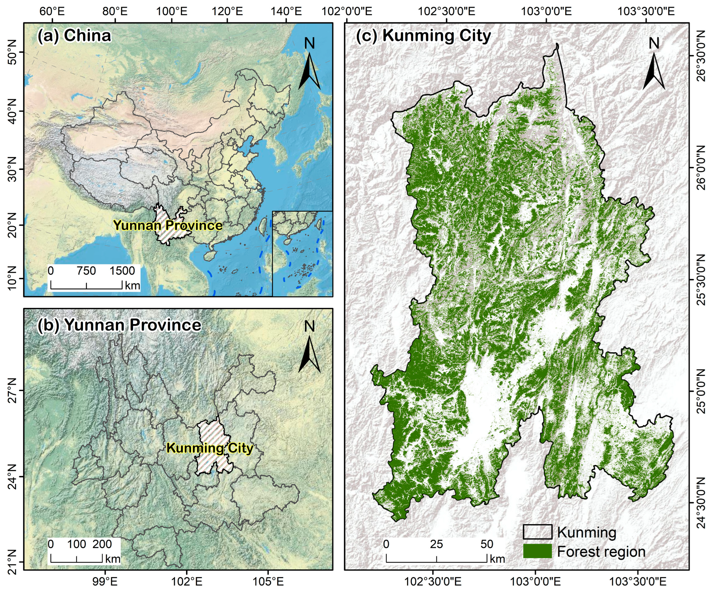
2.1. Overview of the Study Area

Kunming City is situated between 102°10′–103°40′ E and 24°23′–26°22′ N (Figure 1), in the central part of the Yunnan–Guizhou Plateau in southwestern China. With a total area of 21,012.54 km², it serves as the capital of Yunnan Province and the core of the Central Yunnan Urban Agglomeration. Kunming experiences a subtropical plateau monsoon climate, characterized by an average annual temperature of 15 °C and annual precipitation of approximately 1031 mm. Owing to its mild and pleasant climate, the city is often referred to as the “Spring City”. More than 80% of the city’s total area is mountainous. The average elevation of Kunming is approximately 1891 m, with substantial variation across its administrative territory—ranging from a minimum elevation of 746 m to a maximum of 4223 m. According to forest resource monitoring data from 2020, Kunming had a forested area of 10,817 km², corresponding to a forest cover rate of 51.42%. The city’s forest composition is highly diverse, including both natural and plantation forests dominated by species such as Pinus yunnanensis, Quecus spp., Pinus armandii, alder (Alnus spp.), eucalyptus (Eucalyptus spp.), Chinese fir (Cunninghamia lanceolata), poplar (Populus spp.), and walnut (Juglans spp.), alongside other coniferous, broadleaf, and arbor-based economic forests [31].

2.2. Data and Preprocessing

2.2.1. Satellite LiDAR Data

The Advanced Terrain Laser Altimeter System (ATLAS) onboard ICESat-2 utilizes micro-pulse, multi-beam, photon-counting LiDAR technology. It emits laser pulses with a wavelength of 532 nm at a frequency of 10 kHz, generating one pulse approximately every 0.7 m along the ground track. After spectroscopic processing, the laser pulses are divided into three pairs of six beams. The spacing between beam pairs in the cross-track direction is 3.3 km. Each beam pair consists of a strong beam and a weak beam, with an energy ratio of 4:1, and the distance between the two beams in a pair is 90 m. The satellite operates at an altitude of approximately 500 km, with an orbital inclination of 92°, providing global observation coverage between 88° S and 88° N and a revisit period of 91 days [32].

In this study, ICESat-2 data were used to extract discrete measurements of forest canopy height within the study area. Due to the considerable challenges faced by the Level-3 ATL08 product in densely forested, mountainous regions with high canopy closure, this study employed the Level-2 ATL03 product instead. A terrain-adaptive canopy height extraction method, as proposed by Huang et al. [33], was applied to retrieve accurate canopy height information. The extracted canopy height data were subsequently used as training samples to develop and apply an extrapolation model for mapping spatially continuous forest canopy height across the entire study area. The ICESat-2 ATL03 data are publicly available from the official website: https://nsidc.org/data/icesat-2/products (accessed on 23 May 2025).

2.2.2. Optical and Microwave Remote Sensing Data

To enable the spatially continuous retrieval of forest structural parameters, including tree species, stand density, canopy height, and DBH, satellite remote sensing data and their derived products were selected as predictor variables for the extrapolation models. Optical and microwave remote sensing datasets for the year 2020 were obtained from Google Earth Engine (GEE), including imagery from Landsat-8 OLI, Sentinel-1, and Sentinel-2. To represent annual forest conditions, median composite imagery for the year 2020 was generated in GEE to reduce the impact of outliers and cloud contamination. To ensure data quality and temporal consistency, only scenes with cloud cover of less than 10% and acquisition dates closely aligned with ICESat-2 observations were retained.

2.2.3. Optical Remote Sensing Data Derivative Products

This study employed a suite of satellite remote sensing-derived products, including vegetation indices derived from Landsat 8 imagery and global land cover datasets. Given the substantial influence of climatic and geographic conditions on forest growth [34,35], a high-resolution Digital Elevation Model (DEM) from the Shuttle Radar Topography Mission (SRTM) was incorporated to extract topographic variables, such as slope and aspect, for characterizing terrain-related variability in forest structure. In addition, climatic variables, including annual mean temperature and precipitation, were obtained from the WorldClim-2 climate dataset.

2.2.4. Forest Resource Survey Data

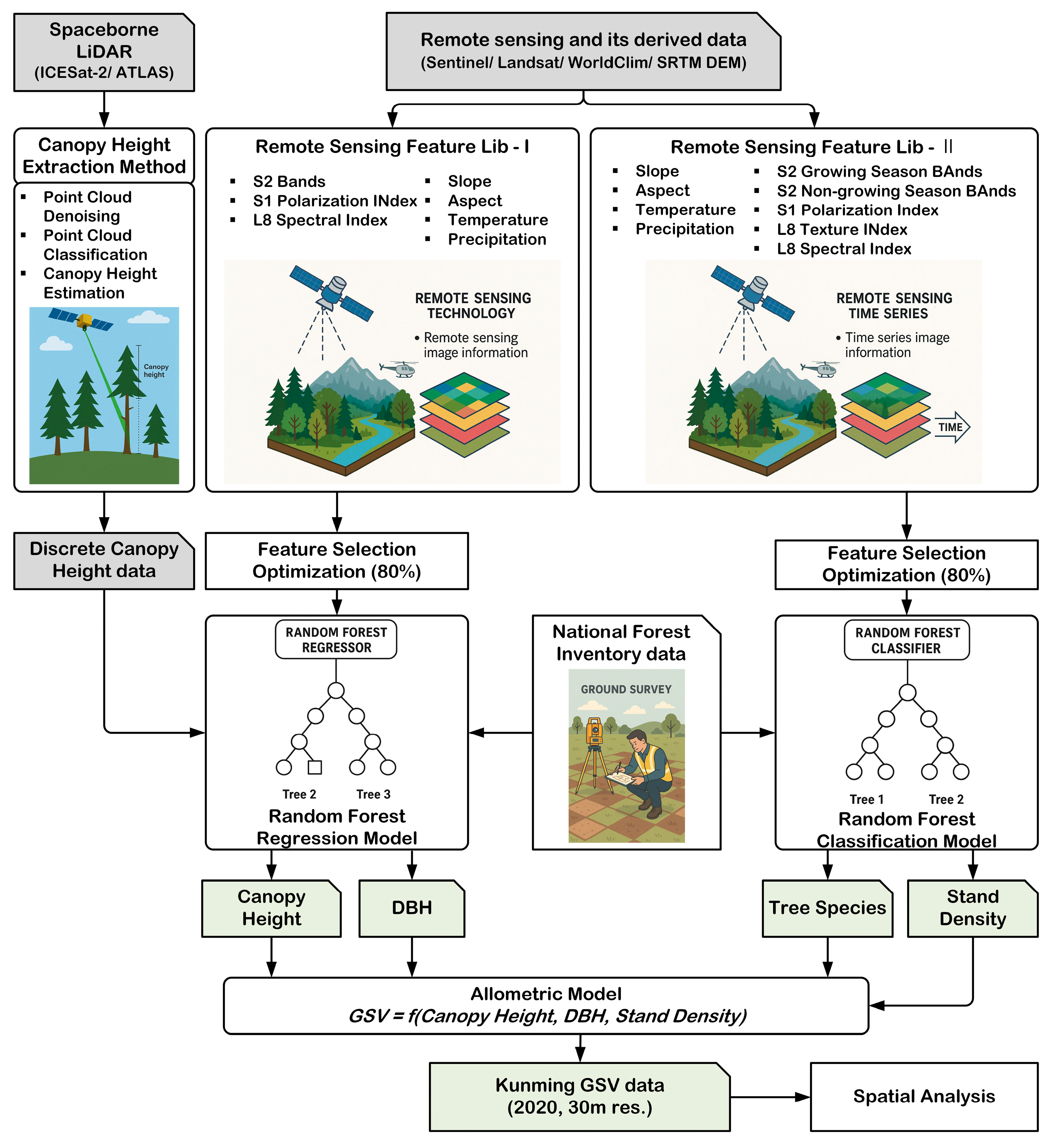
The second-class forest inventory plots used in this study followed the national forest inventory protocol and were established as fixed-area sample plots. In the field, DBH was measured at 1.3 m above ground using diameter tapes, while tree height and stand age were determined using hypsometers and expert knowledge of site history. GSV was calculated based on species-specific allometric equations following the national standard (LY/T 2102-2013) [36], and the number of trees per hectare was derived from stem counts standardized to the plot area. These field-measured attributes served as reference data for model calibration and validation.

Summary statistics of the key stand structural variables used in this study are presented in

Table 1. Summary of key stand attributes derived from second-class forest inventory plots.

Measured Parameters	Unit	Sample Count	Mean	SD	Min	Max	Median
Stand density	trees/pixel	42,834	101.18	45.37	5.22	199.98	98.46
DBH	cm	48,438	10.32	6.24	0.10	52.00	10.00
Canopy height	m	98	11.29	4.03	1.28	20.90	12.00
GSV	m3/ha	48,438	58.09	32.65	1.00	333.90	55.60

. The dataset covers a wide range of stand conditions, with stand density varying from 5.22 to 199.98 trees per pixel, and GSV values ranging from 1.00 to 333.90 m³/ha.

3. Research Methods

This study focuses on the quantitative estimation of growing stock volume (GSV) in Kunming City: (1) extraction of high-accuracy vegetation height samples from ICESat-2/ATLAS photon point clouds using a terrain-adaptive parameterization method, followed by integration with national forest inventory data to construct a robust forest structural parameter sample library encompassing canopy height, DBH, dominant tree species distribution, and stratified stand density classes; (2) implementation of feature engineering based on SAR imagery, optical satellite data, climatic, and topographic variables to identify the most relevant predictors of forest structural parameters. These features, in conjunction with the sample library, are used to train machine learning-based extrapolation models for generating spatially continuous maps of forest structural attributes; and (3) integration of canopy height, DBH, and stand density, together with species-specific allometric equations, to model forest stock volume, thereby enabling accurate estimation and spatial pattern analysis of GSV across the study area. The overall technical workflow of the study is illustrated in Figure 2.

3.1. Forest Structural Parameter Inversion

The forest structural parameters retrieved in this study include dominant tree species, stand density, canopy height, and DBH. Previous studies have demonstrated the effectiveness of integrating multi-source remote sensing data for regional-scale forest structural estimation [37]. Dominant tree species and stand density were classified using random forest classification models, whereas canopy height and DBH were mapped using random forest regression models. A range of feature variables was extracted (

Table 2. Classification feature set of dominant tree species and forest density.

Feature Name	Feature Type and Resolution	Time	Feature Source
VV, VH	Polarization indices, 30 m	Jan–Dec 2020	Sentinel-1
Blue(B2), Green (B3), Red (B4), VRE1 (B5), VRE2 (B6), VRE3 (B7), NIR (B8), VRE4 (B8A), SWIR1 (B11), SWIR2 (B12)	Spectral bands, 30 m	Mar–Sep 2020	Sentinel-2
		Jan–Dec 2020
L8_Second Moment, L8_Entropy, L8_Dissimilarity, L8_Homogeneity, L8_Contrast, L8_Variance, L8_Correlation, L8_Mean	Texture features, 30 m	Sep–Dec 2020	Landsat-8 (by GLCM)
Temperature, Precipitation	Climatic variables, 30 m	2020	WorldClim-2
Elevation, Slope, Aspect	Topographic indices, 30 m	2020	SRTM DEM

and

Table 3. Canopy height and DBH inversion feature set.

Feature Name	Feature Type and Resolution	Time	Feature Source
VV, VH	Polarization indices, 30 m	Jan–Dec 2020	Sentinel-1
Blue(B2), Green (B3), Red (B4), VRE1 (B5), VRE2 (B6), VRE3 (B7), NIR (B8), VRE4 (B8A), SWIR1 (B11), SWIR2 (B12)	Spectral bands, 30 m	Jan–Dec 2020	Sentinel-2
Blue (B2), Green (B3), Red (B4), VRE1 (B5), VRE2 (B6), VRE3 (B7)	Spectral bands, 30 m	Jan–Dec 2020	Landsat-8
L8_RVI (Ratio Vegetation Index), L8_EVI (Enhanced Vegetation Index), L8_NDRE (Normalized Difference Red Edge Index), L8_Ch1NDI (Chlorophyll Normalized Difference Index), L8_DVI (Difference Vegetation Index), L8_NDVI (Normalized Difference Vegetation Index), L8_FDI (Flood Disaster Index), L8_MNDWI (Modified Normalized Difference Water Index), L8_NDWI (Normalized Difference Water Index), L8_NDBI (Normalized Difference Built-up Index), L8_SAVI (Soil-Adjusted Vegetation Index)	Vegetation indices, 30 m
Temperature, Precipitation	Climatic variables, 30 m	2020	WorldClim-2
Elevation, Slope, Aspect	Topographic indices, 30 m	2020	SRTM DEM

), including polarization in-dices derived from Sentinel-1 data, spectral bands from Sentinel-2 and Landsat 8, along with derived vegetation and texture indices. Additionally, topographic indices were generated from DEM data, while climatic variables were obtained from the WorldClim-2 dataset. Different tree species exhibit variation in growth cycles and phenological behavior, with certain species displaying distinct seasonal phenological traits that facilitate classification [38]. In addition, phenological characteristics are linked to tree growth rates and health conditions, which may influence the classification of stand density. High-density stands often exhibit distinctive phenological signatures that reflect their growth status and ecological adaptability [39]. Accordingly, a diverse set of feature variables was selected to support both classification and regression modeling tasks in this study.

3.1.1. Dominant Tree Species and Stand Density Classification

The classification of dominant tree species was based on statistical summaries from the National Forest Inventory and the forest type classification standards outlined in the Technical Regulations for Continuous Forest Inventory (GB/T 38590—2020). Accordingly, the dominant species (or species groups) in the study area were classified into six categories: Pinus yunnanensis, Quercus, Pinus armandii, hard broadleaf species, soft broadleaf species, and other species. In this study, broadleaf species were categorized into two functional groups based on wood hardness: softwood broadleaf species (e.g., willow, Chinese tallow, toon) and hardwood broadleaf species (e.g., oak, elm, Zelkova). This classification follows the conventional grouping used in the national forest inventory to reflect physiological and structural differences. The random forest classification model was constructed as follows:

$$R{F}_{classifier}=Bagging\left({\left\{T_i\left(X_{train}, Y_{train}\right)\right\}}_{i=1}^n, Bootstrap, OOB\right)$$

(1)

where $T_i$ denotes the i-th decision tree; $X_{train}$ is the training data matrix comprising all predictor variables (Table 2); $Y_{train}$ represents the corresponding target variable (tree species class or stand density level); and n is the number of decision trees (ntree), which was set to 100 in this study. The Bootstrap procedure refers to a resampling method in which 80% of the training samples are randomly selected with replacement to construct individual tree subsets. The remaining 20%, referred to as Bootstrap Out-of-Bag (OOB) samples, are used for internal model validation. To enhance the performance of the random forest classification model, the IncNodePurity metric was used to evaluate feature importance. The top 80% of ranked features were retained for final model training [40].

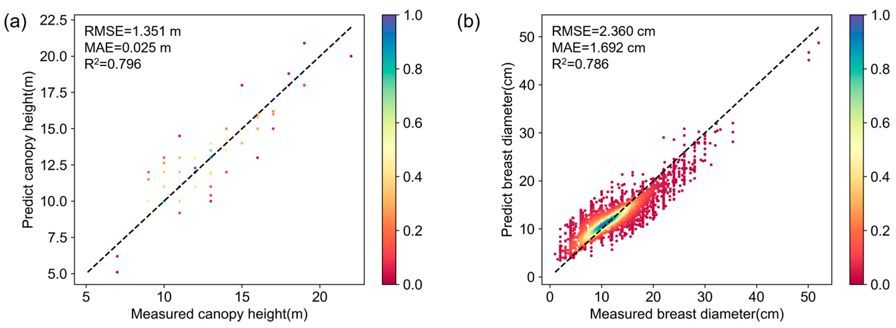
3.1.2. Canopy Height and DBH Inversion

Given that interannual phenological variation has limited influence on canopy height and DBH, phenology-related variables were excluded from the modeling process to avoid feature redundancy. In previous studies, DBH has often been estimated using linear regression based on canopy height. However, the relationship between these two parameters tends to be nonlinear across different forest age stages, potentially introducing estimation errors [41]. Therefore, in this study, canopy height and DBH were modeled independently. The random forest regression model is defined as follows:

$$R{F}_{regressor}=Bagging\left({\left\{T_i\left(X_{train}, Y_{train}\right)\right\}}_{i=1}^n, Bootstrap, OOB\right)$$

(2)

where the target variable refers to continuous values (e.g., canopy height or DBH), and the number of decision trees n was set to 100 in this study.

3.2. Construction of Forest Volume Estimation Model

Allometric models are typically classified into univariate, bivariate, and multivariate forms [42]. Univariate models commonly use DBH as the sole predictor, whereas bivariate models typically incorporate both DBH and canopy height as explanatory variables [43,44]. Previous studies have shown that bivariate models generally yield higher estimation accuracy than univariate models and exhibit broader applicability across various forest types [45]. The allometric model is defined as follows:

$$Y=a{X}^b$$

(3)

where Y represents the dependent variable, such as tree biomass, height, or crown diameter; X denotes the explanatory variable, such as DBH or tree age; and a and b are regression coefficients, representing the scaling constant and the allometric exponent, respectively.

Equation (4) was selected for GSV estimation because it incorporates both DBH and canopy height, which are widely recognized as the most influential structural attributes in forest volume modeling. This multivariate allometric formulation improves the accuracy and generalizability of the estimation compared to univariate models. The model structure and parameterization follow the national standard GB/T 43648–2024: Biomass Models and Carbon Accounting Parameters for Major Tree Species, with species-specific coefficients listed in

Table 4. Allometric model parameters.

Tree Species (Group)	Applicable Conditions	Model Parameters
		a	b	c
Pinus yunnanensis (PY)	DBH < 5 cm	$9.653\times {10}^{-5}$	1.8886	0.79242
	DBH ≥ 5 cm
Pinus armandii (PA)	DBH < 5 cm	$1.4091\times {10}^{-5}$	1.44888	0.90485
	DBH ≥ 5 cm	$9.653\times {10}^{-5}$	1.9114	0.90485
Quercus (QU)	DBH < 5 cm	$1.2939\times {10}^{-4}$	1.48879	0.92394
	DBH ≥ 5 cm	$6.663\times {10}^{-5}$	1.90118	0.92394
Hardwood species (HS)	DBH < 5 cm	$9.033\times {10}^{-5}$	1.49254	1.1359
	DBH ≥ 5 cm	$6.585\times {10}^{-5}$	1.68893	1.1359
Softwood species (SS)	DBH < 5 cm	$7.611\times {10}^{-5}$	1.7653	0.94759
	DBH ≥ 5 cm	$6.175\times {10}^{-5}$	1.89521	0.94759
Other species (OS)	DBH < 5 cm	$1.856\times {10}^{-5}$	1.21398	0.99776
	DBH ≥ 5 cm	$6.799\times {10}^{-5}$	1.83798	0.99776

. Building upon this bivariate allometric model, the present study further incorporates stand density as a correction factor to construct a regional-scale GSV estimation model.

Stand structure refers to the spatial arrangement and physical characteristics of trees within a forest, including attributes such as tree density, species composition, vertical stratification, and DBH distribution. These structural features have a direct influence on the accuracy of canopy height retrieval from remote sensing data. In multi-layered or heterogeneous forests, laser signals may interact with sub-canopy layers or intermediate crowns, potentially causing underestimation of true canopy top height. Since canopy height serves as a key input in allometric equations for GSV estimation, such inaccuracies can propagate through the model and negatively impact volume predictions. Therefore, integrating stand structure as an explanatory factor not only accounts for spatial heterogeneity but also improves the robustness and reliability of GSV modeling across diverse forest conditions.

The final GSV estimation model, integrating stand structure, is expressed as follows:

$$V_{avg}=a\times DB{H}^b\times H^c$$

(4)

$$V_{total}=V_{avg}\times SD$$

(5)

where DBH denotes diameter at breast height, and H represents canopy height; a, b, and c are model parameters. SD refers to stand density, defined as the number of trees per 900 m² pixel (trees/pixel). These values were estimated using predictive models based on remote sensing features, which provide mean structural attributes for each pixel. $V_{avg}$ represents the estimated average forest stock volume per pixel, and $V_{total}$ denotes the total forest stock volume within the pixel.

3.3. Accuracy Validation

The accuracy of the retrieved forest structural parameters was assessed using independent validation datasets. These datasets were primarily derived from ground-based measurements and national forest inventory records. For tree species classification, stand density, DBH, and GSV, 20% of the inventory samples—randomly selected and excluded from model construction—were used for accuracy assessment. As the inventory data did not include canopy height measurements, the accuracy of canopy height retrieval was evaluated using 98 ground-measured field plots, each measuring 30 × 30 m.

(1) The classification accuracy of stand density and dominant tree species was evaluated using confusion matrix analysis, a widely adopted method for accuracy assessment. A confusion matrix was constructed using randomly selected validation samples to evaluate classification performance. Four commonly used metrics were calculated: overall accuracy (OA), producer’s accuracy (PA), user’s accuracy (UA), and the Kappa coefficient.

$$OA={\displaystyle \frac{T{P}_{all}}{P_{all}}}\times 100\%$$

(6)

$$U{A}_{i- tree}={\displaystyle \frac{T{P}_{i- tree}}{P_{i- tree}}}\times 100\%$$

(7)

$$P{A}_{i- tree}={\displaystyle \frac{T{P}_{i- tree}}{C_{i- tree}}}\times 100\%$$

(8)

where $T{P}_{all}$ represents the total number of correctly classified LULC samples; $P_{all}$ is the total number of LULC validation samples. $i-tree$ denotes the i-th tree species category; $T{P}_{i-tree}$ refers to the number of pixels correctly classified as the i-th tree species; $P_{i-tree}$ is the total number of pixels predicted as the i-th tree species; and $C_{i-tree}$ is the total number of reference (validation) pixels for the i-th tree species.

(2) The retrieval accuracy of canopy height, DBH, and GSV was evaluated using three statistical metrics [46]: the coefficient of determination (R²), root mean square error (RMSE), and mean absolute error (MAE). RMSE quantifies the magnitude of overall prediction errors and disproportionately penalizes large deviations, making it highly sensitive to outliers. In contrast, MAE offers a more robust and stable measure of model performance, as it treats all deviations equally and is less influenced by extreme values. The combined use of RMSE and MAE thus provides a more comprehensive and balanced assessment of model accuracy, particularly in heterogeneous forest environments where outlier effects may be present. The corresponding formulas for these metrics are defined as follows:

$$R^2=1-{\displaystyle \frac{\underset{n}{\stackrel{i=1}{\Sigma }}{\left(y_i-{\widehat{y}}_i\right)}^2}{\underset{n}{\stackrel{i=1}{\Sigma }}{\left(y_i-\overline{y}\right)}^2}}$$

(9)

$$RMSE=\sqrt{{\displaystyle \frac{1}{n}}\underset{n}{\stackrel{i=1}{\Sigma }}{\left(y_i-{\widehat{y}}_i\right)}^2}$$

(10)

$$MAE={\displaystyle \frac{1}{n}}\underset{n}{\stackrel{i=1}{\Sigma }}\left|\left(y_i-{\widehat{y}}_i\right)\right|$$

(11)

where n denotes the number of samples; $y_i$ represents the observed (measured) value; ${\widehat{y}}_i$ is the predicted value; and $\overline{y}$ indicates the arithmetic mean of the observed values.

4. Results

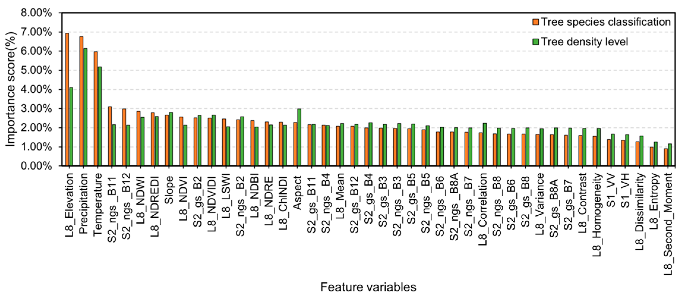
4.1. Feature Importance Results

Given the stochastic nature of the Random Forest algorithm, the mean of IncNodePurity values derived from multiple runs was used as the basis for feature importance ranking in this study. To improve model stability and interpretability, the top 80% of features—ranked by their average IncNodePurity—were selected for model development. This selection was further refined using recursive feature elimination (RFE), ensuring that the most informative variables were retained while minimizing redundancy.

As illustrated in Figure 3, elevation and precipitation consistently emerged as the most important predictors for both tasks, underscoring the strong influence of topographic and climatic conditions on forest structural and compositional variability. In the species classification task, spectral bands from Sentinel-2 (e.g., B11, B12) and vegetation indices such as NDVI and NDWI showed high importance, particularly for broadleaf species. For stand density classification, red-edge indices such as NDRE and ChINDI exhibited greater influence, reflecting their sensitivity to canopy closure and biomass variability.

To further investigate species-specific differences in variable importance, Figure 4 presents the results of feature importance analysis for two regression tasks, tree height prediction (Figure 4a) and DBH estimation (Figure 4b), across multiple tree species. For tree height prediction, topographic variables—especially slope, aspect, and elevation—were consistently ranked among the top predictors across species, particularly for Pinus yunnanensis and Pinus armandii. Climatic factors such as temperature and precipitation also contributed moderately. In contrast, soft broadleaf species demonstrated relatively higher sensitivity to spectral indices, such as NDVI and NDWI, suggesting a closer relationship between canopy reflectance characteristics and height in these species.

In the DBH estimation task, temperature was identified as the most dominant predictor, especially for the “Other tree species” group, where its importance score exceeded 60%. Precipitation also contributed notably for certain broadleaf species. However, spectral bands and vegetation indices generally showed lower importance for DBH estimation compared to their roles in tree height prediction.

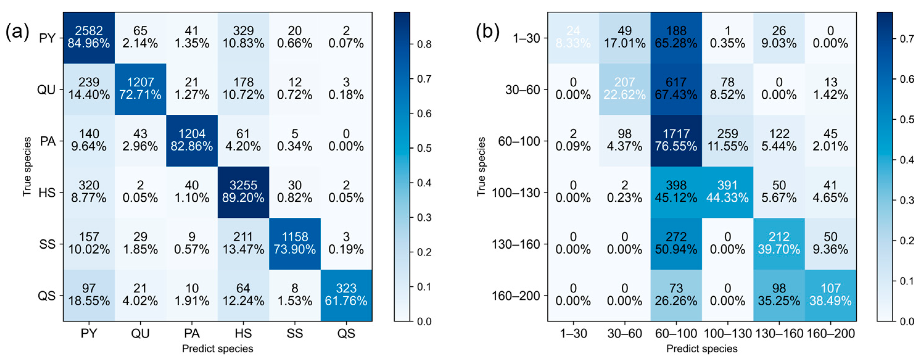
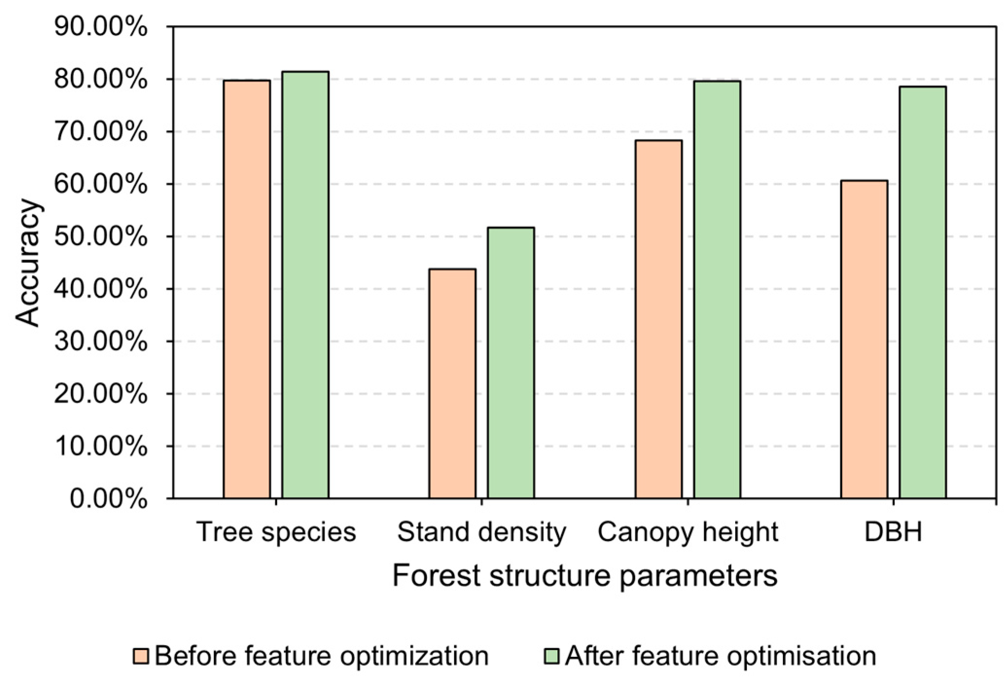
4.2. Accuracy of Results

The retrieval results for dominant tree species, stand density, canopy height, DBH, and GSV were systematically validated for accuracy. Figure 5 presents the classification accuracy for dominant tree species and stand density levels. In Figure 5a, the OA for dominant tree species classification is 81.45%, whereas in Figure 5b, the OA for stand density level classification is 51.74%. Figure 4 illustrates the retrieval accuracy for canopy height and DBH. In Figure 6a, the canopy height model achieved an R² of 0.796, a RMSE of 1.3506 m, and a MAE of 0.9247 m. In Figure 6b, the DBH model yielded an R² of 0.786, a RMSE of 1.6917 cm, and a MAE of 2.3600 cm.

The predicted GSV values were evaluated using independent validation samples, as shown in Figure 7, and the results demonstrated high reliability. The R² was 0.727, with a RMSE of 537.566 m³ and a MAE of 239.767 m³. The predicted GSV values ranged from 0.021 m³ to 189.78 m³, with an average of 8.89 m³ per pixel. Although the predictions tend to be slightly higher than the measured values—particularly at higher stock volumes—the alignment with the 1:1 reference line suggests no substantial systematic bias. This overestimation is a common effect in high-biomass regions, often due to canopy saturation in remote sensing data. Nevertheless, the relatively strong R² value indicates that the model effectively captures the spatial variability and structural patterns of forest stock volume, confirming its robustness and general applicability.

To further evaluate model performance, the estimated total GSV for Kunming City in 2020 was compared with the estimate reported by Wu et al. [47], which was approximately 1.072 × 10⁸ m³. That reference was derived from forest inventory and monitoring data collected during the 13th Five-Year Plan period (2016–2020). Given that our analysis focuses specifically on 2020 conditions, both estimates are temporally consistent. The small discrepancy between them further supports the reliability and accuracy of the model presented in this study.

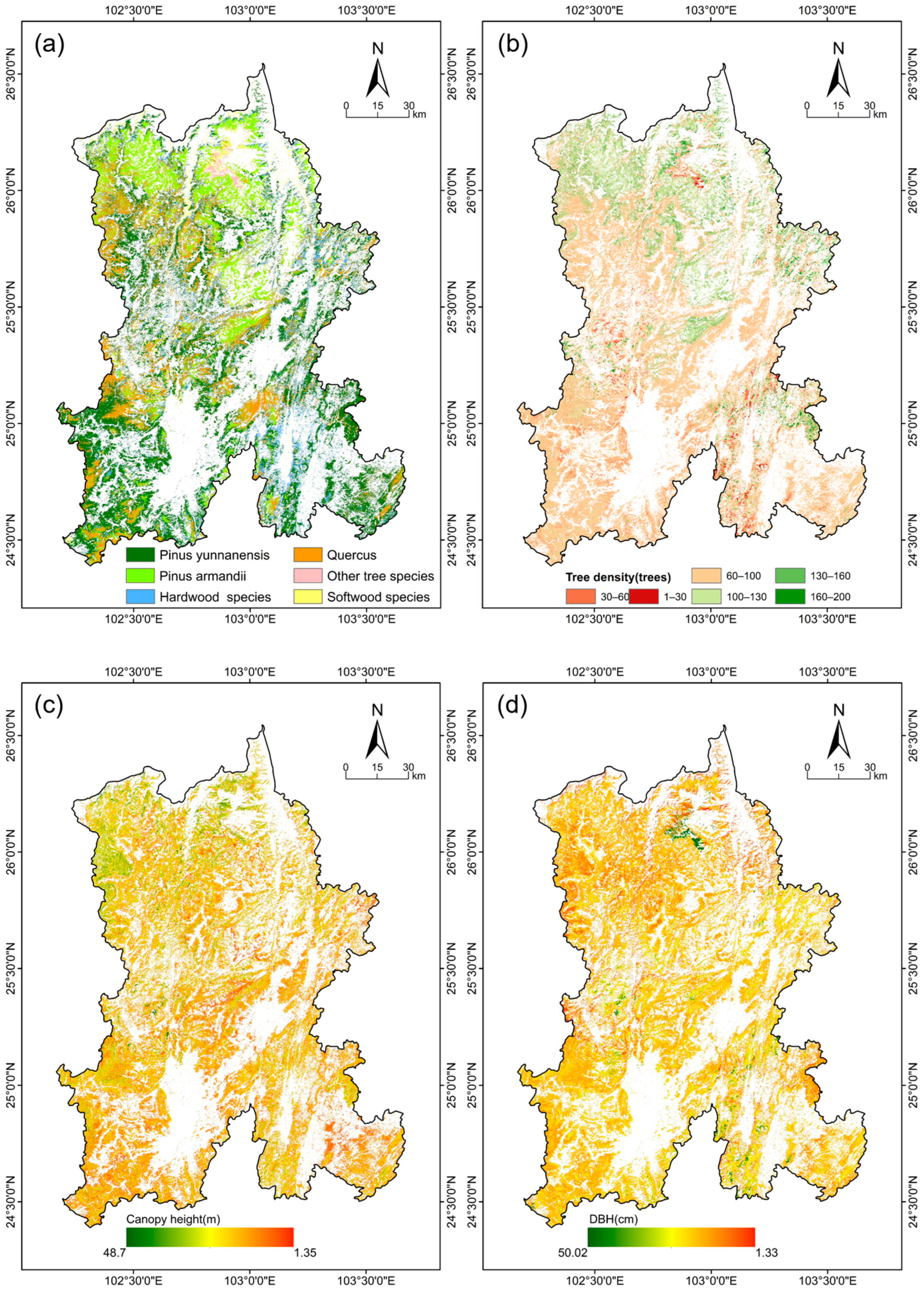
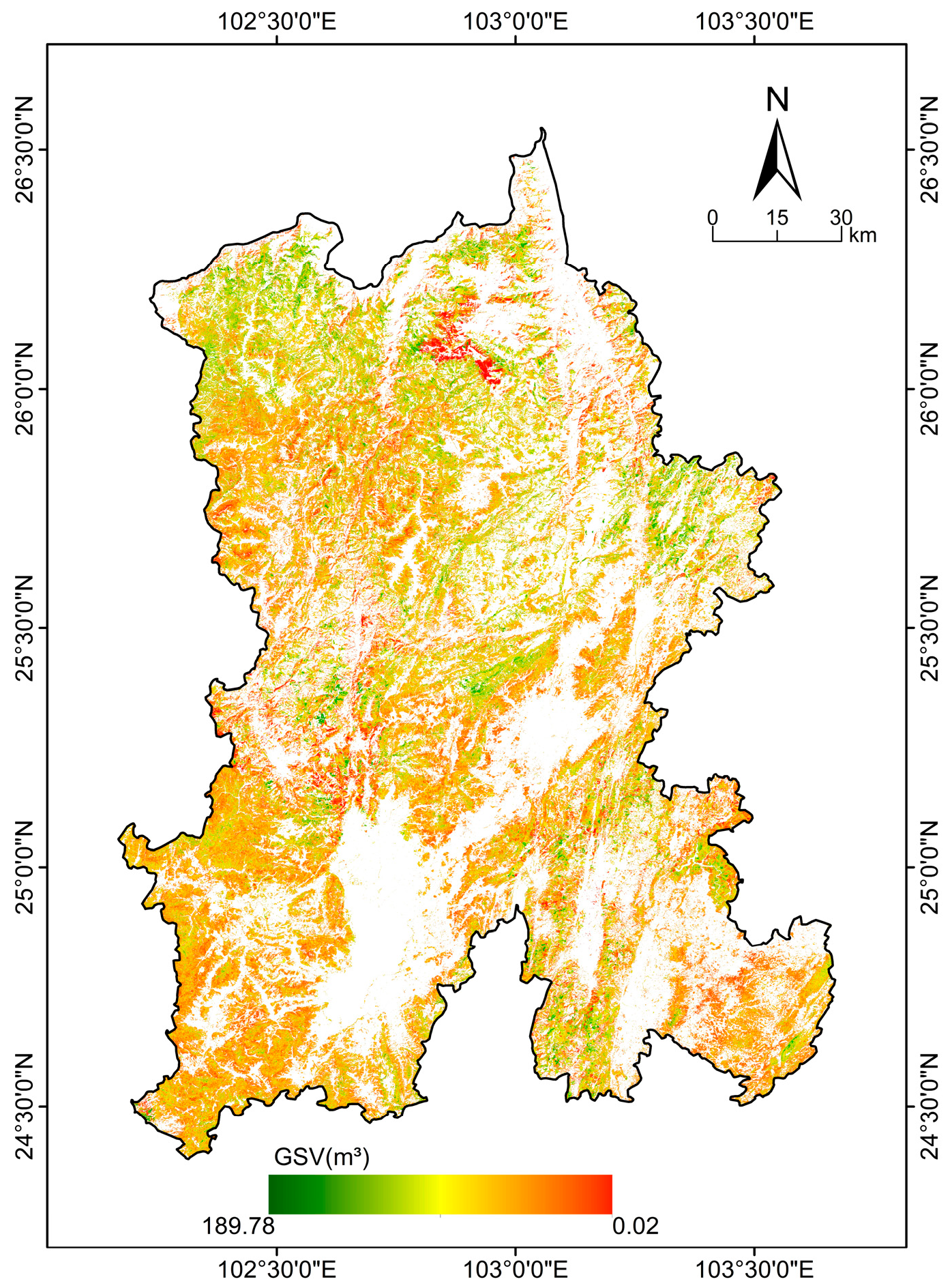
4.3. Forest Structure Parameters and GSV Spatial Continuous Mapping

To construct the classification and regression models, the most relevant image-derived features were selected based on their importance scores. For the classification of dominant tree species and stand density levels, the top 80% of variables ranked by IncNodePurity were selected from Table 2. For the regression of canopy height and DBH, the top 80% of features were similarly selected from Table 3. This approach ensured that only the most informative predictors were used for each specific modeling task. Figure 8a illustrates the spatial distribution and area proportions of the six dominant tree species in Kunming City. Pinus yunnanensis exhibited the widest distribution, accounting for 42.78% of the forested area, followed by Quercus (20.23%), Pinus armandii (17.31%), hard broadleaf species (14.82%), soft broadleaf species (3.92%), and other species (1.15%). Due to variations in site conditions, the same species tend to cluster in localized regions, whereas different species exhibit distinct spatial differentiation. Figure 8b shows that stand density is generally higher in the northern part of Kunming than in the south, primarily because the northern region is mountainous, whereas the southern region is dominated by urban and built-up land. Figure 8c presents the canopy height map predicted using a random forest model based on selected optimal feature variables. The predicted canopy height ranges from 1.35 to 48.7 m, with an average of 15.96 m. Higher canopy heights are observed in the northeastern region, and the overall spatial pattern exhibits a gradual increase from the central area toward the periphery. Figure 8d displays the predicted DBH values, ranging from 1.33 to 50.02 cm, with an average of 11.94 cm.

Based on the model incorporating stand density, the GSV in Kunming City was estimated. The spatial distribution of GSV is illustrated in Figure 9. Statistical analysis indicates that the total GSV in Kunming is approximately 1.01 × 10⁸ m³. The spatial distribution is relatively heterogeneous, exhibiting pronounced regional disparities.

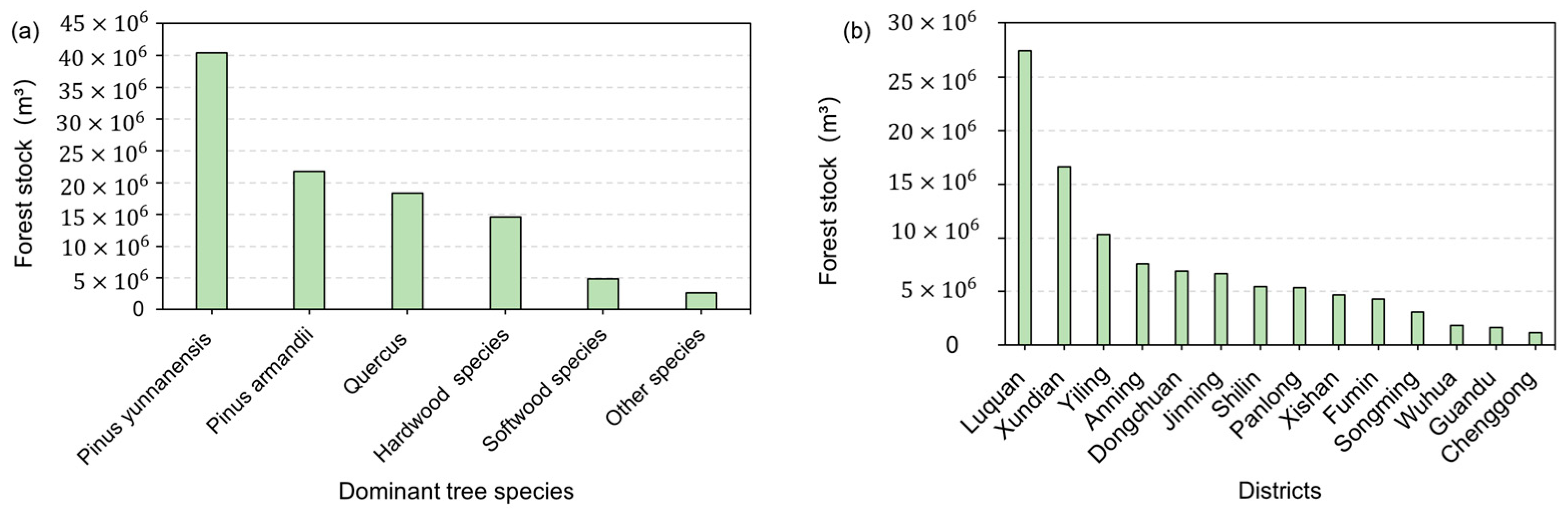
4.4. Spatial Analysis of GSV

As shown in Figure 10, the spatial distribution of GSV in Kunming City was analyzed at both the species and administrative (county/district) levels. Figure 10a presents the distribution of stock volume by tree species. Pinus yunnanensis accounted for the largest share, with 40.40 × 10⁶ m³ (39.34%), followed by Pinus armandii (21.23%), Quercus spp. (17.90%), hard broadleaf species (14.27%), soft broadleaf species (4.69%), and other species (2.58%). Figure 10b illustrates the distribution across 14 counties and districts within Kunming. The highest growing stock volume was found in Luquan Yi and Miao Autonomous County, with 27.45 × 10⁶ m³ (26.68%), followed by Xundian Hui and Yi Autonomous County, with 16.61 × 10⁶ m³ (16.15%). The lowest volume was observed in Chenggong District, totaling only 1.14 × 10⁶ m³ (1.11%).

5. Discussion

5.1. Feature Selection of Model Variables

Previous studies have demonstrated the considerable potential of multi-source remote sensing features in estimating forest structural parameters [48]. In this study, variables derived from spaceborne LiDAR, optical, and microwave sensors were integrated into machine learning models to retrieve forest structural attributes. However, not all input features contribute positively to model performance—redundant or irrelevant variables may introduce noise, increase model complexity, and lead to overfitting [48]. Therefore, feature selection is critical for enhancing both the accuracy and stability of predictive models, as shown in Figure 11, where accuracy significantly increases across all forest structure parameters after feature optimization. From a methodological perspective, the influence of feature selection differs depending on the forest parameter being estimated. For species classification tasks, features related to topography and reflectance—such as elevation, slope, NDVI, and shortwave infrared bands—are particularly relevant, likely due to their ability to capture species-specific ecological niches and canopy spectral responses. In contrast, the estimation of structural parameters such as DBH and canopy height benefits more from moisture-sensitive indices (e.g., NDVI), red-edge bands, and climatic variables, which are more directly linked to biomass accumulation and growth conditions. These distinctions emphasize the importance of aligning feature selection strategies with the ecological processes underlying each modeling objective, rather than applying a one-size-fits-all approach.

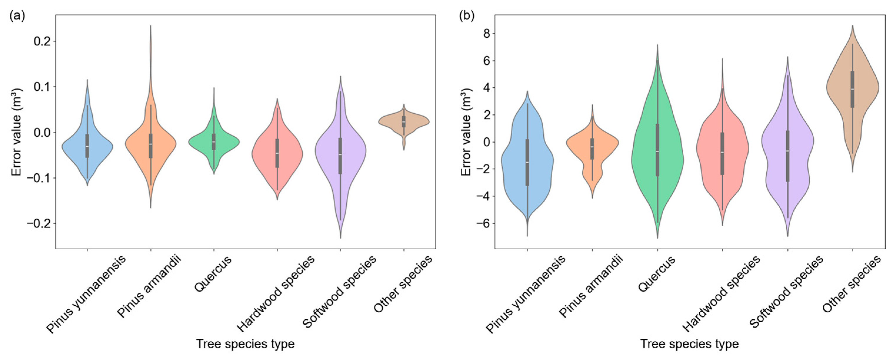
5.2. Impact of Stand Density on GSV Estimation

As shown in

Table 5. Comparison of model accuracy for GSV estimation with and without incorporating stand density (SD) at the pixel level.

Data	R2
Average stock volume (No SD)	0.565
Total stock volume (Increase SD)	0.727

Note. The “Average stock volume (No SD)” model estimates per-tree growing stock volume at the pixel level without incorporating stand density. The “Total stock volume (Increase SD)” model calculates total pixel-level stock volume by multiplying the average stock volume by the estimated stand density (trees per pixel).

, stand density—serving as a key indicator of tree competition and spatial structural characteristics—can significantly enhance the stability and adaptability of allometric models under varying stand conditions.

Previous studies have demonstrated the benefits of incorporating stand density as a predictor variable in remote sensing-based forest inventory models. For example, Li et al. [49] incorporated stand density into GSV estimation models and observed a substantial improvement in model performance, with R² exceeding 0.979—markedly higher than those of models excluding the density variable. Similarly, Domke et al. [50] emphasized that neglecting the effects of stand structural degradation or declining density may lead to systematic overestimation of forest biomass and carbon stocks. Therefore, incorporating stand density into allometric models for regional-scale GSV estimation holds considerable theoretical and practical significance.

As shown in Figure 12, Figure 12a,b illustrates the distribution of estimation errors across different tree species for the traditional isokinetic growth model and the improved model incorporating the stand density parameter, respectively. Figure 12a shows that the traditional model exhibits biased estimation errors and large fluctuations for several species, particularly soft broadleaf species and Quercus spp., where the error distributions are notably asymmetric and the estimation accuracy is unstable. With the introduction of the stand density parameter, the improved model shown in Figure 12b exhibits significantly more convergent estimation error distributions across all species. Overall symmetry improved and the fluctuation range decreased, particularly for Pinus yunnanensis and other species, which showed a marked improvement in accuracy. Although the total GSV of some species still shows a relatively wide error range, the incorporation of stand density significantly improved the overall estimation pattern, yielding more symmetric error distributions and reducing extreme values—particularly for Pinus yunnanensis and other dominant species.

Stand density (SD) is a fundamental structural parameter that influences GSV and above-ground biomass (AGB) by affecting canopy closure, tree competition, and vertical structure. Its importance is especially evident in heterogeneous forests, where structural variability arises from species composition, stand age, and disturbance history. Incorporating SD into remote sensing-based models has been shown to significantly improve estimation accuracy and ecological relevance. Prior studies have reported strong correlations between SD and biomass estimates (e.g., R² = 0.910 in tropical forests; Wassihun et al. [51]), and have demonstrated that SD enhances the stability and generalizability of machine learning models across diverse forest types and regions (Fassnacht et al. [52]; Chen et al. [53]; Lehmann et al. [54]).

In our study, pixel-level SD, derived from national forest inventory data, was dynamically integrated into a random forest framework for regional-scale GSV estimation. This spatially explicit modeling strategy overcomes the limitations of generalized allometric models and effectively mitigates the mixed-pixel effects commonly encountered in remote sensing imagery, where forest and non-forest land covers coexist within a single pixel [55]. By incorporating SD, the model suppresses spectral interference from non-forest elements such as shrubs, grasslands, or bare ground, thereby improving the reliability of volume estimates. Moreover, the inclusion of SD enables the model to capture structural dynamics such as the self-thinning process observed in natural forest development, where stand density typically decreases with forest age while average biomass per tree increases [56,57,58]. Accounting for these age-related variations enhances the ecological realism of the model and contributes to improved estimation performance. As demonstrated in Table 5, this approach yielded a substantial gain in predictive accuracy, with the R² increasing from 0.565 to 0.727. These results reinforce the dual role of SD—as both a structural descriptor and a critical explanatory variable—in enhancing model performance for large-scale forest stock assessments.

6. Conclusions

The GSV estimation model developed in this study, which incorporates stand density, demonstrated satisfactory accuracy when applied to Kunming City. The key findings are as follows:

(1)

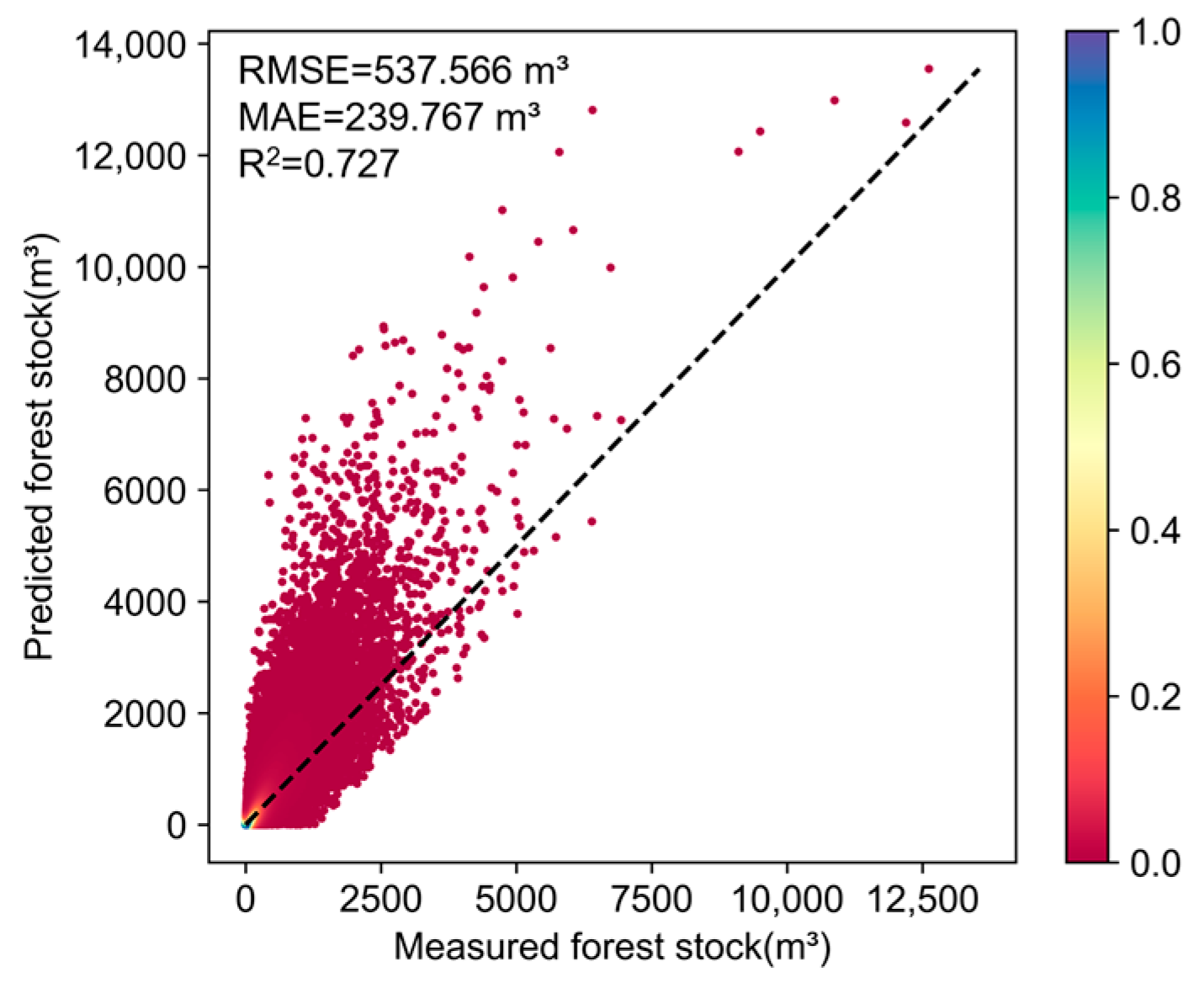
The total GSV in Kunming was estimated at 1.01 × 10⁸ m³. Validation against national forest inventory data confirmed the reliability of the results (R² = 0.727);

(2)

The integration of stand density into the GSV estimation model significantly improved overall accuracy. Specifically, it elevated R² from 0.565 to 0.727 and notably reduced the RMSE and MAE values. This result highlights the critical role of stand density as an explanatory variable, particularly in heterogeneous forest environments, and supports its inclusion to enhance model robustness at large scales;

(3)

Spatial analyses at both the species and administrative levels revealed significant heterogeneity in GSV distribution. This study provides a novel technical approach for supporting national forest inventory efforts and offers a cost-effective, efficient, and accurate method for regional GSV estimation. It also provides valuable decision-making support for forest resource management in Kunming City.

Although key variables were identified through feature importance analysis, further optimization of the feature selection process remains warranted. Future studies may incorporate methods such as L1 regularization or principal component analysis (PCA) to mitigate the effects of multicollinearity. With ongoing advancements in remote sensing and phenological observation technologies, the use of high-resolution time-series data is expected to further enhance model performance. In addition, to address error accumulation in GSV estimation, greater emphasis should be placed on data quality control and model parameter optimization to reduce the influence of uncertainty on final outcomes.

References

1. Sun, L.L.; Cui, H.J.; Ge, Q.S. Will China achieve its 2060 carbon neutral commitment from the provincial perspective? Adv. Clim. Change Res. 2022, 13, 169–178. [Google Scholar] [CrossRef]
2. Guohua, L.; Bojie, F.; Jingyun, F. Carbon dynamics of Chinese forests and its contribution to global carbon balance. Acta Ecol. Sin. 2000, 20, 732–740. [Google Scholar]
3. Pan, Y.; Birdsey, R.A.; Fang, J.; Houghton, R.; Kauppi, P.E.; Kurz, W.A.; Phillips, O.L.; Shvidenko, A.; Lewis, S.L.; Canadell, J.G.; et al. Daniel Hayes, A Large and Persistent Carbon Sink in the World’s Forests. Science 2011, 333, 988–993. [Google Scholar] [CrossRef] [PubMed]
4. Somogyi, Z.; Teobaldelli, M.; Federici, S.; Matteucci, G.; Pagliari, V.; Grassi, G.; Seufert, G. Allometric biomass and carbon factors database. Ifor.-Biogeosci. For. 2008, 1, 107–113. [Google Scholar] [CrossRef]
5. Hu, Y.; Xu, X.; Wu, F.; Sun, Z.; Xia, H.; Meng, Q.; Huang, W.; Zhou, H.; Gao, J.; Li, W.; et al. Estimating Forest Stock Volume in Hunan Province, China, by Integrating In Situ Plot Data, Sentinel-2 Images, and Linear and Machine Learning Regression Models. Remote Sens. 2020, 12, 186. [Google Scholar] [CrossRef]
6. Santoro, M.; Beaudoin, A.; Beer, C.; Cartus, O.; Fransson, J.E.S.; Hall, R.J.; Pathe, C.; Schmullius, C.; Schepaschenko, D.; Shvidenko, A.; et al. Forest growing stock volume of the northern hemisphere: Spatially explicit estimates for 2010 derived from Envisat ASAR. Remote Sens. Environ. 2015, 168, 316–334. [Google Scholar] [CrossRef]
7. Liu, M.Y.; Nie, S.; Wang, C.; Xi, X.; Cheng, F.; Feng, B. Forest stock volume inversion based on ICESat-2 and Sentinel-2A data. Remote Sens. Nat. Resour. 2024, 36, 210–216. [Google Scholar] [CrossRef]
8. Ma, T.; Hu, Y.; Wang, J.; Beckline, M.; Pang, D.; Chen, L.; Ni, X.; Li, X. A Novel Vegetation Index Approach Using Sentinel-2 Data and Random Forest Algorithm for Estimating Forest Stock Volume in the Helan Mountains, Ningxia, China. Remote Sens. 2023, 15, 1853. [Google Scholar] [CrossRef]
9. Li, W.; Niu, Z.; Shang, R.; Qin, Y.; Wang, L.; Chen, H. High-resolution mapping of forest canopy height using machine learning by coupling ICESat-2 LiDAR with Sentinel-1, Sentinel-2 and Landsat-8 data. Int. J. Appl. Earth Obs. Geoinf. 2020, 92, 102163. [Google Scholar] [CrossRef]
10. Huang, X.; Cheng, F.; Wang, J.; Yi, B.; Bao, Y. Comparative study on remote sensing methods for forest height mapping in complex mountainous environments. Remote Sens. 2023, 15, 2275. [Google Scholar] [CrossRef]
11. Astola, H.; Häme, T.; Sirro, L.; Molinier, M.; Kilpi, J. Comparison of Sentinel-2 and Landsat 8 imagery for forest variable prediction in boreal region. Remote Sens. Environ. 2019, 223, 257–273. [Google Scholar] [CrossRef]
12. Ding, X.Y.; Chen, E.X.; Zhao, L.; Fan, Y.; Xu, K.; Ma, Y. An allometrie method for estimating above ground biomass based on airbore LiDAR and spaceborne multispectral data. Remote Sens. Nat. Resour. 2024, 3, 1–10. Available online: https://link.cnki.net/urlid/10.1759.p.20240731.1702.014 (accessed on 23 May 2025).
13. Luo, Y.; Lin, G.; Song, Y.; Shi, K.; Xu, J. Binary Standing Volume Model for Pinus amandii in Yunnan Province. For. Invent. Plan. 2024, 49, 12–18. [Google Scholar] [CrossRef]
14. Wang, Z.C.; Du, H.; Song, T.Q.; Peng, W.X.; Zeng, F.P.; Zeng, Z.X.; Zhang, H. Allometric models of major tree species and forest biomass in Guangxi. Acta Ecol. Sin 2015, 35, 4462–4472. [Google Scholar] [CrossRef]
15. West, G.B.; Brown, J.H.; Enquist, B.J. A general model for the origin of allometric scaling laws in biology. Science 1997, 276, 122–126. [Google Scholar] [CrossRef]
16. Han, W.X.; Fang, J.Y. Review on the mechanism models of allometric scaling laws: 3/4 vs. 2/3 power. Chin. J. Plant Ecol. 2008, 32, 951–960. [Google Scholar] [CrossRef]
17. Lu, D.; Chen, Q.; Wang, G.; Liu, L.; Li, G.; Moran, E. A survey of remote sensing-based aboveground biomass estimation methods in forest ecosystems. Int. J. Digit. Earth 2016, 9, 63–105. [Google Scholar] [CrossRef]
18. Fang, J.Y.; Liu, G.H.; Xu, S.L. Biomass and net production of forest vegetation in China. Acta Ecol. Sin. 1996, 16, 497–508. [Google Scholar]
19. Kittredge, J. Estimation of the amount of foliage of trees and stands. J. For. 1944, 42, 905–912. [Google Scholar]
20. Woodwell, G.M.; Whittaker, R.H.; Reiners, W.A.; Likens, G.E.; Delwiche, C.C.; Botkin, D.B. The Biota and the World Carbon Budget: The terrestrial biomass appears to be a net source of carbon dioxide for the atmosphere. Science 1978, 199, 141–146. [Google Scholar] [CrossRef]
21. Zeng, W.S. Development of monitoring and assessment of forest biomass and carbon storage in China. For. Ecosyst. 2014, 1, 20. [Google Scholar] [CrossRef]
22. Li, Q.; Liu, Z.; Jin, G. Impacts of stand density on tree crown structure and biomass: A global meta-analysis. Agric. For. Meteorol. 2022, 326, 109181. [Google Scholar] [CrossRef]
23. Cai, H.; Di, X.; Chang, S.X.; Jin, G. Stand density and species richness affect carbon storage and net primary productivity in early and late successional temperate forests differently. Ecol. Res. 2016, 31, 525–533. [Google Scholar] [CrossRef]
24. Chave, J.; Réjou-Méchain, M.; Búrquez, A.; Chidumayo, E.; Colgan, M.S.; Delitti, W.B.C.; Duque, Á.; Eid, T.; Fearnside, P.M.; Goodman, R.C.; et al. Improved allometric models to estimate the aboveground biomass of tropical trees. Glob. Change Biol. 2014, 20, 3177–3190. [Google Scholar] [CrossRef] [PubMed]
25. Thom, D.; Rammer, W.; Albrich, K.; Braziunas, K.H.; Dobor, L.; Dollinger, C.; Hansen, W.D.; Harvey, B.J.; Hlásný, T.; Hoecker, T.J.; et al. Parameters of 150 temperate and boreal tree species and provenances for an individual-based forest landscape and disturbance model. Data Brief 2024, 55, 110662. [Google Scholar] [CrossRef]
26. McRoberts, R.E.; Næsset, E.; Gobakken, T. Inference for LiDAR-assisted estimation of forest growing stock volume. Remote Sens. Environ. 2013, 128, 268–275. [Google Scholar] [CrossRef]
27. Dean, T.J.; D’Amato, A.W.; Palik, B.J.; Battaglia, M.A.; Harrington, C.A. A direct measure of stand density based on stand growth. For. Sci. 2021, 67, 103–115. [Google Scholar] [CrossRef]
28. Yun, T.; Jiang, K.; Li, G.; Eichhorn, M.P.; Fan, J.; Liu, F.; Chen, B.; An, F.; Cao, L. Individual tree crown segmentation from airborne LiDAR data using a novel Gaussian filter and energy function minimization-based approach. Remote Sens. Environ. 2021, 256, 112307. [Google Scholar] [CrossRef]
29. Cheng, K.; Yang, H.; Chen, Y.; Yang, Z.; Ren, Y.; Zhang, Y.; Lin, D.; Liu, W.; Huang, G.; Xu, J.; et al. How many trees are there in China? Sci. Bull. 2025, 70, 1076–1079. [Google Scholar] [CrossRef]
30. Crowther, T.W.; Glick, H.B.; Covey, K.R.; Bettigole, C.; Maynard, D.S.; Thomas, S.M.; Smith, J.R.; Hintler, G.; Duguid, M.C.; Amatulli, G.; et al. Mapping tree density at a global scale. Nature 2015, 525, 201–205. [Google Scholar] [CrossRef]
31. Weinan, Z.; Yong, W.; Guanglong, O. Remote Sensing Estimation and Inversion of Biomass for Major Forest Types in Kunming Based on Landsat 8 OLI. J. Southwest For. Univ. 2023, 43, 107–116. [Google Scholar] [CrossRef]
32. Markus, T.; Neumann, T.; Martino, A.; Abdalati, W.; Brunt, K.; Csatho, B.; Farrell, S.; Fricker, H.; Gardner, A.; Harding, D.; et al. The Ice, Cloud, and land Elevation Satellite-2 (ICESat-2): Science requirements, concept, and implementation. Remote Sens. Environ. 2017, 190, 260–273. [Google Scholar] [CrossRef]
33. Huang, X.; Cheng, F.; Wang, J.; Duan, P.; Wang, J. Forest canopy height extraction method based on ICESat-2/ATLAS data. IEEE Trans. Geosci. Remote Sens. 2023, 61, 5700814. [Google Scholar] [CrossRef]
34. Gao, W.Q.; Liu, J.F.; Xue, Z.M.; Zhang, Y.T.; Gao, Z.H.; Ni, Y.Y.; Wang, X.F.; Jiang, Z.P. Geographical patterns and drivers of growth dynamics of Quercus variabilis. For. Ecol. Manag. 2018, 429, 256–266. [Google Scholar] [CrossRef]
35. Vicente-Serrano, S.M.; Camarero, J.J.; Azorin-Molina, C. Diverse responses of forest growth to drought time-scales in the Northern Hemisphere. Glob. Ecol. Biogeogr. 2014, 23, 1019–1030. [Google Scholar] [CrossRef]
36. National Technical Committee on Forest Resources of Standardization Administration of China (SAC/TC 370). Tree Biomass Models and Related Parameters to Carbon Accounting for Major Tree Species. GB/T 43648-2024; Standards Press of China: Beijing, China, 2024. Available online: https://d.wanfangdata.com.cn/standard/ChpTdGFuZGFyZE5ld1MyMDI1MDUxMzE3MDEzOBIPR0IvVCA0MzY0OC0yMDI0GghqZzExYnRxMw (accessed on 23 May 2025).
37. Li, H.; Hiroshima, T.; Li, X.; Hayashi, M.; Kato, T. High-resolution mapping of forest structure and carbon stock using multi-source remote sensing data in Japan. Remote Sens. Environ. 2024, 312, 114322. [Google Scholar] [CrossRef]
38. Blickensdörfer, L.; Oehmichen, K.; Pflugmacher, D.; Kleinschmit, B.; Hostert, P. National tree species mapping using Sentinel-1/2 time series and German National Forest Inventory data. Remote Sens. Environ. 2024, 304, 114069. [Google Scholar] [CrossRef]
39. Wu, X.; Niu, C.; Liu, X.; Hu, T.; Feng, Y.; Zhao, Y.; Liu, S.; Liu, Z.; Dai, G.; Zhang, Y.; et al. Canopy structure regulates autumn phenology by mediating the microclimate in temperate forests. Nat. Climate Change 2024, 14, 1299–1305. [Google Scholar] [CrossRef]
40. Deng, Y.; Pan, J.; Wang, J.; Liu, Q.; Zhang, J. Mapping of Forest Biomass in Shangri-La City Based on LiDAR Technology and Other Remote Sensing Data. Remote Sens. 2022, 14, 5816. [Google Scholar] [CrossRef]
41. Zhu, X. Forest Height Retrieval of China with a Resolution of 30 m Using ICESat-2 and GEDI Data; University of Chinese Academy of Sciences: Beijing, China, 2021; Volume 4, p. 2020. [Google Scholar]
42. West, G.B.; Brown, J.H.; Enquist, B.J. A general model for the structure and allometry of plant vascular systems. Nature 1999, 400, 664–667. [Google Scholar] [CrossRef]
43. Ketterings, Q.M.; Coe, R.; van Noordwijk, M.; Ambagau, Y.; Palm, C.A. Reducing uncertainty in the use of allometric biomass equations for predicting above-ground tree biomass in mixed secondary forests. For. Ecol. Manag. 2001, 146, 199–209. [Google Scholar] [CrossRef]
44. Kaitaniemi, P. Testing the allometric scaling laws. J. Theor. Biol. 2004, 228, 149–153. [Google Scholar] [CrossRef] [PubMed]
45. Wang, K.; Shu, Q.; Zhao, H.; Tan, D.; Yuan, Z. Model Uncertainty Analysis of Aboveground Biomass Estimation of Pinus densata. J. Southwest For. Univ. 2021, 41, 100–106. [Google Scholar] [CrossRef]
46. Foody, G.M. Status of land cover classification accuracy assessment. Remote Sens. Environ. 2002, 80, 185–201. [Google Scholar] [CrossRef]
47. Wu, Y.; Zan, J.; Liao, C.; Leng, H.; Shi, K.; Zhang, Z.; Wang, H. Analysis of forest resource changes in Yunnan Province: Taking forest resource changes during the 13th Five-Year Plan as an example. Green Sci. Technol. 2022, 24, 169–172. [Google Scholar] [CrossRef]
48. Huang, H.; Liu, C.; Wang, X.; Zhou, X.; Gong, P. Integration of multi-resource remotely sensed data and allometric models for forest aboveground biomass estimation in China. Remote Sens. Environ. 2019, 221, 225–234. [Google Scholar] [CrossRef]
49. Li, J.; Xiong-qing, Z.; Ai-guo, D. Develop Annual Stand Volume Growth Model of Chinese fir Including Different Stand Density Indices. For. Sci. Res. 2022, 35, 97–102. [Google Scholar] [CrossRef]
50. Domke, G.M.; Woodall, C.W.; Smith, J.E. Accounting for density reduction and structural loss in standing dead trees: Implications for forest biomass and carbon stock estimates in the United States. Carbon Balance Manag. 2011, 6, 14. [Google Scholar] [CrossRef]
51. Wassihun, A.N.; Hussin, Y.A.; Van Leeuwen, L.M.; Latif, Z.A. Effect of forest stand density on the estimation of above ground biomass/carbon stock using airborne and terrestrial LIDAR derived tree parameters in tropical rain forest, Malaysia. Environ. Syst. Res. 2019, 8, 27. [Google Scholar] [CrossRef]
52. Fassnacht, F.E.; Mangold, D.; Schäfer, J.; Immitzer, M.; Kattenborn, T.; Koch, B.; Latifi, H. Estimating stand density, biomass and tree species from very high resolution stereo-imagery–towards an all-in-one sensor for forestry applications? For. Int. J. For. Res. 2017, 90, 613–631. [Google Scholar] [CrossRef]
53. Chen, L.; Ren, C.; Zhang, B.; Wang, Z.; Liu, M.; Man, W.; Liu, J. Improved estimation of forest stand volume by the integration of GEDI LiDAR data and multi-sensor imagery in the Changbai Mountains Mixed forests Ecoregion (CMMFE), northeast China. Int. J. Appl. Earth Obs. Geoinf. 2021, 100, 102326. [Google Scholar] [CrossRef]
54. Tian, H.; Zhu, J.; He, X.; Chen, X.; Jian, Z.; Li, C.; Ou, Q.; Li, Q.; Huang, G.; Liu, C.; et al. Using machine learning algorithms to estimate stand volume growth of Larix and Quercus forests based on national-scale Forest Inventory data in China. For. Ecosyst. 2022, 9, 100037. [Google Scholar] [CrossRef]
55. Hsieh, P.F.; Lee, L.C.; Chen, N.Y. Effect of spatial resolution on classification errors of pure and mixed pixels in remote sensing. IEEE Trans. Geosci. Remote Sens. 2001, 39, 2657–2663. [Google Scholar] [CrossRef]
56. Jinghui, M. A comparison of different methods for fitting the self-thinning equation. J. Beijing For. Univ. 2019, 41, 58–68. [Google Scholar] [CrossRef]
57. Aiguo, D.; Lihua, F.; Jianguo, Z. Self-thinning rules at Chinese fir (Cunninghamia lanceolata) plantations—Based on a permanent density trial in southern China. J. Resour. Ecol. 2019, 10, 315–323. [Google Scholar] [CrossRef]
58. Ogawa, K. Mathematical consideration of the age-related decline in leaf biomass in forest stands under the self-thinning law. Ecol. Model. 2018, 372, 64–69. [Google Scholar] [CrossRef]
Figure 1. Overview of the study area.
Forests 16 00891 g001
Figure 2. Technical flow chart.
Forests 16 00891 g002
Figure 3. Importance map of tree species classification and stand density classification features.
Forests 16 00891 g003
Figure 4. Importance map of tree height and DBH inversion features. (a) Canopy height; (b) DBH.
Forests 16 00891 g004
Figure 5. Confusion matrix of measured data and predicted results. (a) Tree species; (b) Stand density level (trees /pixel). In each cell, the upper value indicates the number of pixels, and the lower value indicates the corresponding classification percentage. The color gradient represents the number of pixels, with darker colors indicating higher counts. Diagonal elements represent correctly classified samples.
Forests 16 00891 g005
Figure 6. Regression density plot of canopy height and DBH. (a) Canopy height; (b) DBH.
Forests 16 00891 g006
Figure 7. GSV accuracy verification diagram.
Forests 16 00891 g007
Figure 8. Spatial distribution of different forest structure parameters in Kunming. (a) Tree species; (b) Stand density; (c) Canopy height; (d) DBH.
Forests 16 00891 g008
Figure 9. Spatial distribution of GSV in Kunming City.
Forests 16 00891 g009
Figure 10. Spatial distribution of GSV in Kunming. (a) Distribution of different dominant tree species; (b) Distribution in different districts and counties.
Forests 16 00891 g010
Figure 11. Comparison of accuracy before and after optimization of each parameter feature.
Forests 16 00891 g011
Figure 12. Comparison of the impact of stand density on the estimation accuracy of GSV volume. (a) Average GSV; (b) Total GSV.
Forests 16 00891 g012