Article

Bark Stripping Damage Caused by Red Deer (Cervus elaphus L.): Inventory Design Using Hansen–Hurwitz and Horvitz–Thompson Approach

by
Christoph Hahn
1,2 and
Sonja Vospernik
1,*
1
Institute of Forest Growth, BOKU University (University of Natural Resources and Live Sciences, Vienna), 1180 Wien, Austria
2
Forestry School Traunkirchen (Forstfachschule des Bundes Traunkirchen in OÖ), 4801 Traunkirchen, Austria
*
Author to whom correspondence should be addressed.
Forests 2025, 16(6), 890; https://doi.org/10.3390/f16060890
Submission received: 12 April 2025 / Revised: 11 May 2025 / Accepted: 23 May 2025 / Published: 25 May 2025
(This article belongs to the Section Forest Inventory, Modeling and Remote Sensing)

Abstract

:
This study investigates the use of adaptive cluster sampling (ACS) for estimating bark stripping damage in forests, employing the Hansen–Hurwitz (HH) and Horvitz–Thompson (HT) estimators. Through simulations, we analysed the total, summer, and new bark stripping damage with varying grid sizes and sample sizes in eight full-censused stands in Northern Styria/Austria. The results showed that the HT estimator consistently had lower standard errors (SEs) (variability of the sample mean from the true population mean) than the HH estimator. SEs decreased with increasing grid space for new and summer damages, but increased for total damage up to 35 m, then remained stable. Inclusion probabilities (IP) were highest for total damage. ACS showed precision gains, particularly for rare and clustered damages like new damage, but did not achieve the target SE of 10%. Adaptive sampling is most beneficial for monitoring rare and clustered events, though precision remains limited, especially for new damage. The study suggests ACS is suitable for rare damage types (e.g., summer and new bark stripping wounds) but requires further refinement to meet operational precision targets. Future work should focus on integrating adaptive designs with practical field methods, such as fixed-radius plots and refined damage criteria.

1. Introduction

1.1. Bark Stripping Damage as Ecological and Economical Factor

Bark stripping damage caused by red deer (Cervus elaphus L.) is a significant factor in European forest ecosystems and is also of interest to forest management companies. In many regions of central Europe, red deer populations are tending towards overabundance [1], leading to an increase in bark stripping damage [2,3]. This damage can result in high economic losses [4] and reduce the stability of forest stands against wind and snow breakage [5] due to subsequent fungal infections [6]. Additionally, bark stripping can decrease tree growth [7]. In central Europe, winter bark stripping damage is prevalent [8,9,10,11]. However, information about summer damage is also valuable in forest inventories due to its higher impact on trees. Summer damages are generally larger in size [10,11,12], and the teeth marks are not visible because the bark can be easily peeled off in larger pieces from the stem [13]. Since the probability of wound infection with wood-destroying fungi is linearly related to the wound length [14,15], infection rates are higher for summer bark stripping damage. Also, the decay rate decreases with the age of the wounds [16]. Mechanical damage, in general, increases the risk of bark beetle outbreaks [17], particularly for Ips typographus (L.). Larger wounds, especially those caused by summer bark stripping, can significantly elevate the risk of bark beetle damage.

1.2. Importance of Bark Stripping Assessments

Selecting an appropriate sampling design for the required accuracy is a critical step in designing a forest inventory. This selection depends on the frequency and distribution of the variable(s) of interest [18,19]. For essential variables, the Global Climate Observing System mandates an inferential uncertainty of not more than 20% [20]. This threshold is necessary to prevent forest management and policy-makers from being misled by analysis and drawing incorrect conclusions [21]. Traditional forest inventory methods are designed to evaluate characteristics like tree volume, basal area or stem number variables that are widespread and exhibit a uniform distribution across the area (evenly distributed) [22]. In contrast, additional variables like tree damage, volume of dead wood or biodiversity indicators, are often clustered or rare and can thus not be effectively assessed using traditional methods [22].
To address these limitations, various methods have been developed to assess more complex and less evenly distributed variables. For instance, several methods for assessing bark stripping intensity are included in various national forest inventories [2,22,23,24]. For instance, the National Forest Inventory in Austria (ÖWI) uses angle count samples with a basal area factor of 4 m2/ha and a maximum plot area of 300 m2 to assess bark stripping damage [24]. The benefit of this framework is the reduced field work and the reduction of the non-detection bias [25]; Tokola and Shresthaba [26] compared different cluster-sampling techniques for forest inventory in southern Nepal for the assessment of rare events: They examined different numbers of points per cluster (1, 2, 3, 4, 5 and 8 Points/Cluster) and cluster types (point, line, triangle, L-shape and square). Distance sampling was used to assess deadwood in managed forests [27], habitat trees [28,29] and low abundance tree species in tropical forests [30] and can be integrated into existing forest inventories [31].
All the above methods can be used for the assessment of bark stripping damage and are well-established and have been used in various inventories. While these methods outline major trends in bark stripping intensity, assessing new bark stripping damage provides more accurate and recent data on the impact of ungulates on ecosystems [32]. A threshold for new bark stripping rates can be established [19,33] to serve as the basis for compensation payments to ensure precise monitoring and management decisions [32,33]. Moreover, two-stage sampling approaches are designed for the inventory of rare and clustered events, such as new bark stripping. An example is the post-stratification of inventory data based on remote sensing, which can be used for efficient analyses of regional-level results from operational National Forest Inventories and for smaller areas accurately [34].

1.3. Adaptive Sampling with Hansen–Hurwitz and Horvitz–Thompson Estimator

1.3.1. ACS and Network Development

ACS is a viable method for rare and clustered characteristics, such as bark stripping damages. The basic idea involves fully tessellating the area and taking an initial sample (n1) randomly without replacement. If the initial sample satisfies a specific condition, the neighbouring points (north, south, east, and west) are also included in the sample. If any of these neighbouring points also meet the condition, their neighbours are subsequently analysed. This procedure continues until no neighbouring points meet the condition. As a result, irregular networks of sample points are created, each either surrounded by potential sample points with no damaged trees (“edge units”) or by the border of the stand. These networks and their edge units are collectively referred to as a cluster. If an initial sample does not meet the criterion (i.e., it does not contain damaged trees), its neighbours are not analysed, and this sampling unit is defined as a cluster of size one without edge units [35,36]. These networks/clusters have varying probabilities, of being selected by the initial sample.

1.3.2. Inclusion Probability in ACS; Hansen–Hurwitz and Horvitz–Thompson Estimator

When conducting adaptive sampling, we need to distinguish between the first-order probability (αi) that a sample i intersects a network and the second-order probability (α*) that points from the same cluster are included in the sample. Consequently, the selection of the previous point(s) influences the probabilities of subsequent points. The first-order probability [37] is generally given by
α i = 1 N m i n 1 N n 1
where
  • N: Number of all potential sample points
  • mi: Number of sample points in the network Ai
  • n1: number of the initial sample.
The second-order probability, which is the joint inclusion probability for the two networks, is given by Equation (2). It is difficult to calculate in practice because of the sampling design without replacement, where the probability changes with every draw.
α j k = 1 N m j n 1 + N m k n 1 N m j m k n 1 N n 1
where
  • αjk: second-order probability for the networks j and k.
Both the Hansen–Hurwitz and the Horvitz–Thompson estimators are widely used in adaptive sampling. The Hansen–Hurwitz estimator provides a simple and robust approach for estimating the population mean or total when samples are selected randomly. It is especially useful for “unequal probability sampling” [38]. It is defined as:
μ ^ H H = 1 n 1 i = 1 n 1 w i
with
w i = 1 m i a = 1 n N W y a
where
  • μ ^ H H : Estimator for the mean
  • wi: mean of yi-values in the mi observed networks
  • nNW: number of sample points in the network m
  • ya: observed y-values of the sample points in the network m.
Following Thompson and Seber [39], the mean estimate of HH can be considered as the sample mean of a sample with size n1 and the sample values of wi. This calculation method yields an unbiased estimator of the variance given by
v a r ^ μ ^ H H = N n 1 N n 1 n 1 1 i = 1 n 1 w i μ ^ H H 2
The Horvitz–Thompson estimator is also widely used in situations where the sample elements are known, but potentially unequal. It is a generalisation of the Hansen–Hurwitz estimator, making it especially flexible and powerful [40]. In general, the Horvitz–Thompson estimator has been shown to be more efficient [37], although there may be cases where the Hansen–Hurwitz estimator is more efficient [41]. The HT-estimator is given by
μ ^ H T = 1 N k = 1 K y k * α k
where
  • y k * : sum of the y-values in the kth network
  • αk: 1st order inclusion probability of the network k
  • K: number of distinct networks intersected by the initial sample n1.
The calculation of the variance of the HT-estimator is challenging in practice, particularly because the second-order probability is required. In situations with fixed sample sizes, the variance formula in the Sen–Yates–Grundy form is preferred as it avoids negative variance estimations [42]:
v a r ^ S Y G μ ^ H T = i ,   j S i < j π i π j π i j π i j y i π i y j π j 2
where
  • πi and πj: 1st order prob. for the networks i and j to be in the sample S
  • yi and yj: sum of the y-values in the jth and kth networks
  • πij: 2nd order inclusion probability of the networks j and k.
Nevertheless, this approach does not resolve the issue of the second-order probability. To calculate the second-order probability, approximation techniques are necessary. Such methods provided by Deville [43] or Berger [44], are designed for various situations and have their own advantages and disadvantages. Other estimators, such as Murty’s estimator and the Rao–Blackwell estimator, also consider edge units [45].

1.4. Advantages of Adaptive Sampling

From a sampling point of view, both bark stripping damage and new bark stripping damage have several properties that make assessment with systematic inventory methods inefficient [23,32]. Both types of damage are concentrated on young stands of preferred tree species, and within stands, the damage is clustered [12,46]. Additionally, new bark stripping damage is a rare phenomenon. While the first two properties suggest a stratified sampling design, for rare and clustered target variables, adaptive sampling approaches are proposed [36].
Adaptive cluster sampling is a design-unbiased sampling method that is particularly efficient for sampling rare and spatially clustered populations. It can be used with different sampling designs such as simple random sampling, systematic sampling, stratified sampling [47], inverse sampling [48], two-stage sampling [49], double sampling [50], and designs with or without replacement of clusters [45]. Further, it can be applied to sampling with equal probability [51] and unequal probability [22], such as angle count sampling [22,52,53].
Adaptive sampling is widely used in biological studies for rare and clustered research objects such as animals (e.g., waterfowl [54]), fish (e.g., shellfish [55], lampreys [56], fish eggs [57]), aquatic studies (e.g., sediment load in rivers [58], hydroacoustic surveys [59]), and plants (e.g., low abundance [60], seaweed [61], herpetofauna [62]). In forest science, it is used for deforestation rates [63], sparse forest populations [64], and rare tree species [22].
For such situations, i.e., for rare populations with aggregation tendencies, dispersal patterns and environmental patchiness it has been shown that adaptive sampling is more efficient than systematic sampling. If the population is truly rare and clustered, substantial gains in precision of up to 50% have been reported [22]. Gains in precision in adaptive sampling increase with a higher degree of clustering, and gains are larger the larger the areas where the event is encountered [22,51,64].

1.5. Disadvantages of Adaptive Sampling

In sampling, both precision and the cost of the sampling strategy are important concerns. Estimates of the marginal cost of adapting must be balanced against the benefit of an improved estimate. If the variable of interest is truly rare, additional costs are minor. The requirement that the trait is rare is one of practicality, not necessity from a statistical point of view [22]. In practice, it may be uncertain, whether the variable of interest is rare or clustered [64].
When adaptive sampling is used and the population is neither clustered nor rare, adaptive sampling has disadvantages: if it is not clustered, adaptive estimators are no better than non-adaptive ones but are more cost intensive. For non-rare sampling, overestimation is common. Because the sample size is unknown beforehand, planning of fieldwork is difficult. To apply adaptive sampling to more frequent and clustered variables and to reduce the risk of oversampling, stratification and partitioning into blocks [36], a two-stage ACS that takes information from a pilot study into account [45], restricted ACS [65], stopping rules [57,66], data-driven stopping rules [67], conditional expansion [51], and generalised adaptive sampling [68] have been proposed.
While for most of these measures, both the Hansen–Hurwitz and the Horvitz–Thompson estimators have been shown to be design-unbiased, some (e.g., fixed stopping rules) are not unbiased for these two estimators and require other estimators such as Murty’s estimator.

1.6. Hypotheses

In this article, we aim to address the following hypotheses:
  • Adaptive cluster sampling is more accurate for estimating bark stripping, summer bark stripping damage, and new bark stripping damage for both the Hansen–Hurwitz and Horvitz–Thompson estimators.
  • Gains in precision are higher for new bark stripping damage than for summer bark stripping damage and total bark stripping damage because it is a rare event. Estimates from the Horvitz–Thompson estimator are computationally more demanding but more precise.

2. Materials and Methods

2.1. Study Area and Data

The eight analysed forest stands are located in the forest company “Wasserberg” in Gaal/Austria (Latitude: 47.2°; Longitude: 15.1°) at an elevation ranging from 1009 to 1622 m. The stands are primarily composed of pole stands of Norway spruce (Picea abies (L.) Karst.) with minor admixtures of European larch (Larix decidua Mill.). Figure 1 gives an overview of the location of the stands.
A full census was conducted in these stands from 2019 to 2020. Each of the eight stands was scanned with a laser scanner (FARO Focus3D X330”—Faro Technologies Inc., Lake Mary, FL, USA). The scan parameters were set on multiscan mode with resolution parameter = 1/4 (resolution r = 6.136 mm/10 m) and the quality parameter was defined as 4x (measuring time = 8 µs/scan point). After co-registration, the tree coordinates were calculated automatically from the point clouds by an algorithm developed at the Institute of Forest Growth [69,70,71].
The subsequent field assessment involved verifying the calculated coordinates and assessing the following data for each tree and bark-stripping wound:
  • Tree species;
  • Diameter at breast height (DBH) [cm];
  • Tree height calculated from height curves [m];
  • Wound characteristics (visually classified):
    Damage type (summer or winter damage);
    Damage age (old damage or new damage);
    Wound length (max. vertical extent) [cm];
    Wound width (max. horizontal extent) [cm].
Summer damage occurs during the vegetation period (spring and summer) when the bark can be peeled off easily, resulting in larger bark strips (possibly over 1 m in length) with jagged wound edges and minimal or no visible tooth marks. Winter damage occurs during the vegetation-free period (autumn and winter) when sap flow is absent, making the bark harder to remove. This results in smaller wounds, often grouped together, with clearly visible tooth marks. Additionally, we defined new damage as damage not older than one year, characterised by little to no wound healing, minimal callus tissue, and often fresh resin (especially in Norway spruce). Old damage was defined as damage older than one year, with visible wound healing, significant callus tissue, and largely dried resin. For graphical examples of the various damage types and ages, we refer to the excellent work of Reimoser and Reimoser [72]. Detailed information about the measurement procedures is provided by Hahn and Vospernik [12].
The stands cover areas between 0.31 and 1.77 hectares, with stem densities ranging from 495 to 1507 stems per hectare. On average, 22.1% of the volume is affected by bark stripping, with 0.4% being new damage and 2.9% being summer bark stripping damage. Detailed information about the damage rates for all stands is provided in Table 1. The Supplementary Material includes detailed maps of the spatial distribution of the trees and damage types (Figures S1–S3).

2.2. Software

All calculations for this paper were performed using R statistical software (version 4.1.2), with the scripts specifically developed for this project by the authors.

2.3. Tessellation and Sampling Scenarios

The aim of the study was to compare different sampling schemes for bark stripping inventories using adaptive sampling without replacement, evaluated with the Hansen–Hurwitz (HH) and the Horvitz–Thompson estimators (HT). To enable this comparison, it was necessary to pre-define the grid space for tessellation and the number of initial sampling units n1, which were randomly selected without replacement from all possible sampling units. The sampling scenarios were defined as all possible combinations of the following parameters:
  • Grid space of the potential sample points (GS) ranged from 10 to 50 m (step: 5 m).
  • The number of the initial sampling units (n1) ranged from 2 to 6 points per stand (step: 1).
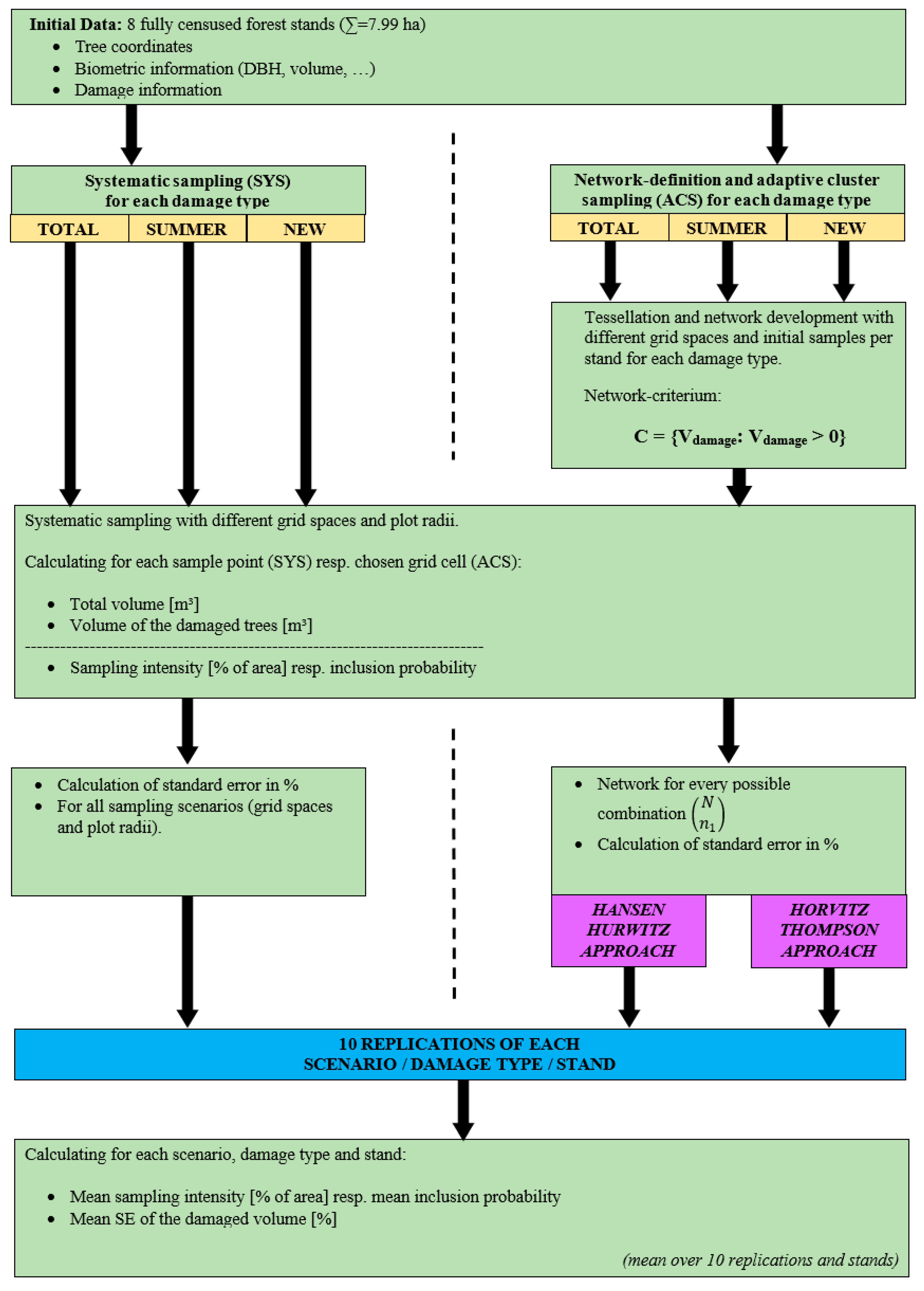
To account for the randomness in grid placement, each scenario was replicated 10 times with different randomly located grids, and the average of the results was calculated. For all scenarios and replications, the following steps were performed:
1.
The area of the eight stands was tessellated into squares based on the specified grid space.
2.
For each square, both total tree volume and volume of damaged trees were calculated (formulas for this are provided in the Appendix A).
3.
All possible N n 1 combinations of n1 initial sample points were drawn without replacement.
4.
Network development was carried out for all combinations using the criterion C = {Vdamage: Vdamage > 0}; meaning that if at least one bark-stripped tree was included in the sample, the four adjacent points (north, east, south, and west) were added and analysed. This process continued until no further neighbouring points met the criterion.
5.
For each scenario and replication, both the Hansen–Hurwitz and Horvitz–Thompson estimators, as well as their respective standard errors (SE), were calculated.

2.4. Evaluation of Hansen–Hurwitz (HH) and Horvitz–Thompson (HT) Estimator

As described in the introduction, the calculation of the variance of the HT estimator is difficult because all combinations of n1 have to be taken into account. Nevertheless, in our case, it was possible to calculate all possible combinations because the areas of our eight separate stands are quite small (Table 1). Therefore, we used the calculation approach given by Salehi and Seber [45] and used Formulas (8)–(17).
All calculations were performed for total damages (TOTAL), summer damages (SUMMER) and new damages (NEW) separately. A calculation example for the probability pi that a sample point is chosen in the adaptive approach is given in the Supplementary Material.
Network-Development:
j = N n 1
m e a n n = i = 1 j n N W ,   i p i
I P = n N W N
Hansen–Hurwitz:
w = 1 n N W i = 1 n N W y i
H H i = 1 n 1 i = 1 n 1 w i
μ H H = i = 1 j H H i p i
v a r H H = i = 1 j H H i μ H H 2 p i
Horvitz–Thompson:
H T = 1 j i = 1 n N W y i a I a p a
μ H T = i = 1 j H T i p i
v a r H T = i = 1 j H T i μ H T 2 p i
where
  • N: Number of potential sample points derived from the grid;
  • n1: Number of sample points of the initial sample;
  • j: Number of possible combinations from n1 initial sample points from N potential sample points;
  • pi: Probability of a network to be chosen by n1 initial sample points and subsequent network development;
  • yi: value of the analysed variable. In our case, the volume of the damaged trees [m] in the grid cell; separately for TOTAL, SUMMER and NEW damage;
  • nNW: Number of the sample points in the network(s);
  • mean(n) mean number of sample points chosen through the network development starting from n1.
As results, the standard error in percent of the mean was defined. Therefore, it was calculated using the results above as
S E H H = v a r H H m e a n _ n N W 2
resp.
S E H T = v a r H T m e a n _ n N W 2
and
S E % H H = 100 S E H H μ H H
resp.
S E % H T = 100 S E H T μ H T
where
  • SEHH: HH-standard error of the sampling scenario;
  • SEHT: HT-standard error of the sampling scenario;
  • mean_nNW: Mean sample points in the chosen networks;
  • µHH resp. µHT: mean damaged volume calculated by HH estimator resp. HT estimator;
  • SE(%)HH resp. SE(%)HT: Standard error of the HH estimator resp. HT estimator in percent of the mean damaged volume.
This calculation was performed for all stands and for all 10 replications. As a final result, the SE in percent (for HH and HT resp.) and the inclusion probability were calculated as the mean over the eight stands and over the ten replications.

2.5. Systematic Sampling—Calculation

To compare the precision of the adaptive sampling with the HH and HT estimator, the inventory was also calculated as systematic sampling with fixed radius plots with different grid spaces (10 to 50 m) and different radii (2 to 10 m). Details about this calculation can be seen by Hahn and Vospernik [32].

2.6. Graphical Overview

A graphic overview of the calculation steps carried out in this paper is given in Figure 2.

3. Results

3.1. HH Estimator and HT Estimator

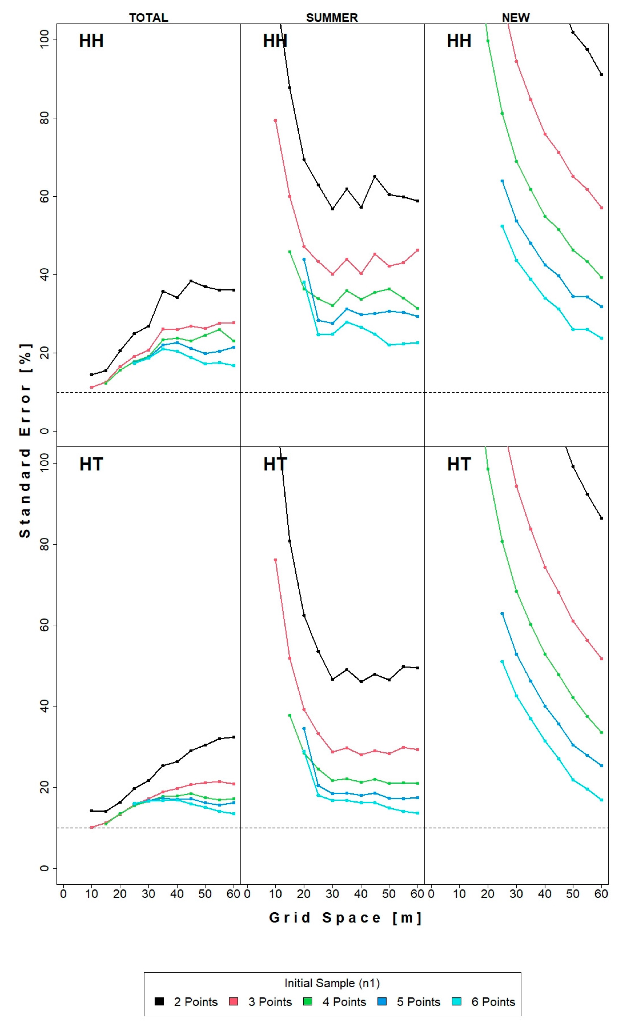
Figure 3 displays the standard error (SE) [%] of the Hansen–Hurwitz estimator and the Horvitz–Thompson estimator for different damage types. Standard errors were on average smallest for total bark stripping damage, followed by summer bark stripping damage and new bark stripping damage. The range of standard errors was considerable for both Hansen–Hurwitz and Horvitz–Thompson estimators and ranged between >10% and 40% for total bark stripping damage, 15% and >100% for summer bark stripping damage and between 20% and >100% for new bark stripping damage. In our examples, no scenario reached the target precision of 10% SE. Total damage increased with increasing grid space until approximately 35 m. Subsequently, the SE remains constant or slightly decreases. Differences between scenarios became larger with increasing grid space and an increasing number of initial sample points. Trends differed for summer damage and new damage. As grid space increased, the standard error decreased. Further, an increase in the initial sample size typically resulted in a decrease in standard error. When comparing the two estimators, the Horvitz–Thompson estimator yielded lower SEs in all cases.

3.2. Inclusion Probability

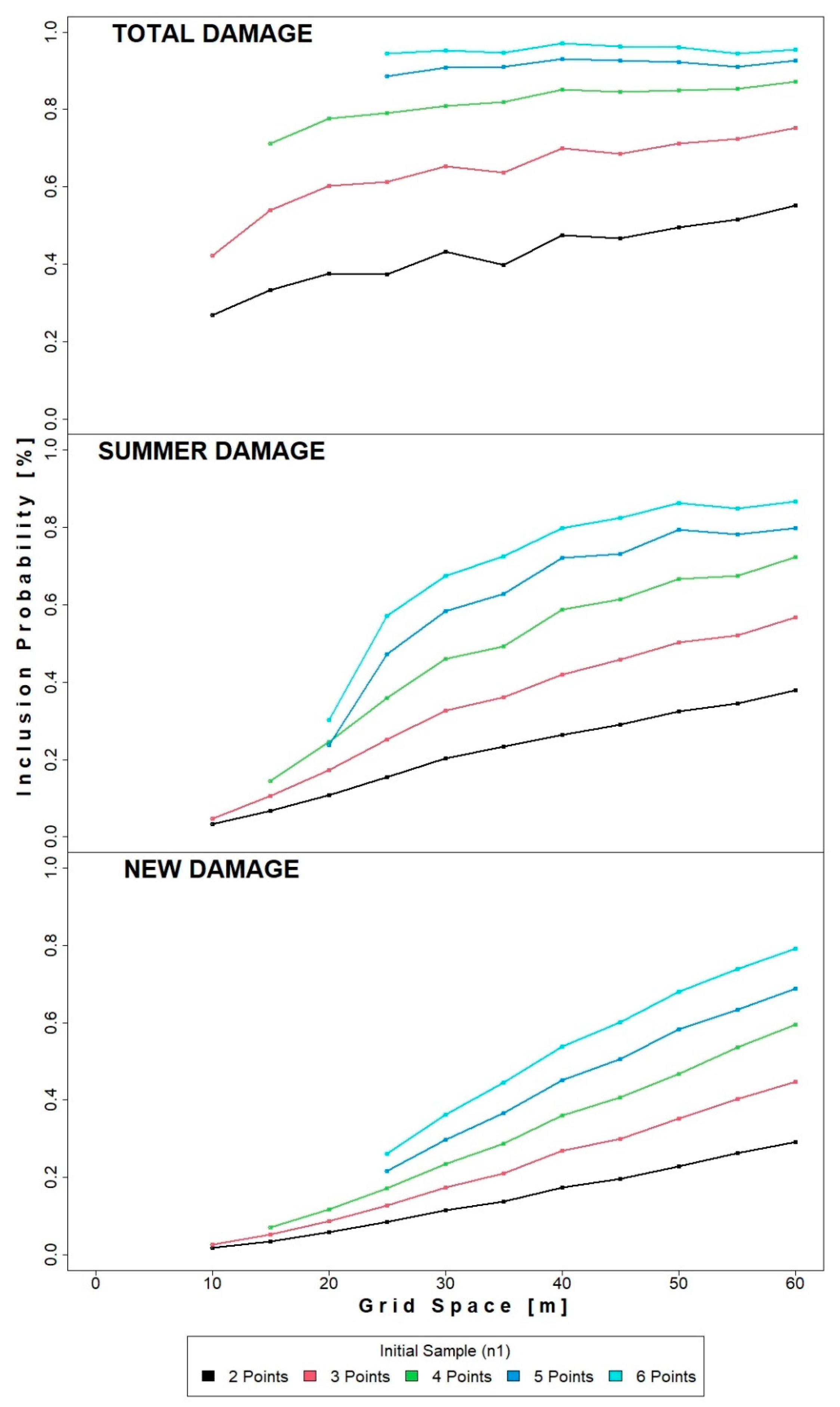
The inclusion probability (IP) increased with the grid space in all cases, especially in sampling scenarios with a high number of initial samples (Figure 4). This effect is particularly pronounced for new and summer damages. In all cases, the IP is highest for total damage, followed by summer damage and new damage. For different numbers of initial sample plots, the IP is higher for scenarios with higher n1.

3.3. Systematic Sampling—Results

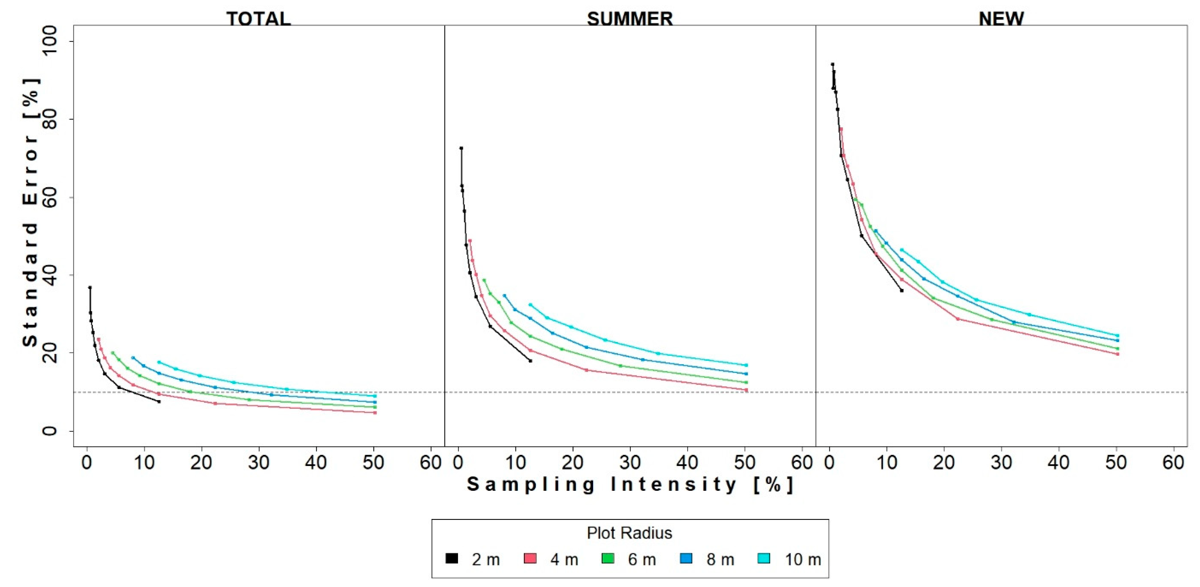
The results of the systematic sampling are shown in Figure 5 for total damage (left), summer damage (middle) and new damage (right). In all scenarios, the standard error is lowest for total and highest for new bark stripping damage. For total bark stripping damages, a standard error of less than 20% can be reached with a high number of small grid spaces. For summer damage and new damage, this target cannot be achieved. In all cases, a high number of small sample plots is more precise than a lower number with a higher plot radius at the same sampling intensity.
Note that in systematic sampling, the grid space and the radius of the sampling scheme directly determine the sampling intensity (e.g., a grid space of 25 m and a plot radius of 4 m leads to 10000 25 2 = 16 sample points per ha and a mean sampling intensity of 100 × 16 × 4 2 π 10000 = 8.04 % ).

4. Discussion

4.1. Precision and Efficiency

Systematic sampling is often inefficient for clustered and/or rare populations [23,32]. Adaptive cluster sampling aims to provide more precise estimates for these cases [36]. Generally, the Horvitz–Thompson Estimator produces a lower standard error than the Hansen–Hurwitz Estimator. This is consistent with the findings of several authors (e.g., [37,45]), who favour the HT estimator for this reason. The different damage types analysed in this study exhibit varying precisions and inclusion probabilities when using adaptive cluster sampling. For total damage rates, the inclusion probability was smaller than for the summer damages and smallest for new damages. The least gain in precision was found for total damage, moderate improvement was observed for summer damage and the greatest improvement was observed for new damage. An increase in rareness and potential clustering is observed when comparing total damage, summer damage, and new damage, as reflected by the precision gain [22,51,64].
The degree of clustering and rareness is also crucial for the limitations of the adaptive design: For non-rare events, like the total bark stripping damage rate, avoiding oversampling is challenging, especially for a high number of initial sample points (n1), for rare events, such as the new bark stripping rate, acceptable sampling intensities can be achieved even with a higher n1 [73].
Adaptive cluster sampling was found to be more effective than simple random sampling (SRS) for the assessment of clustered populations [64]. Talvitie et al. [64] also emphasised that larger population clusters yield greater efficiency when measuring and estimating the variables of interest. Furthermore, they point out that very small networks can be disadvantageous in ACS. This aligns with our findings that more sample points are needed to obtain precise estimates of target variables in the case of rare or strongly clustered events.
For summer and new damages, the SE becomes high, especially for small grid spaces. This can be explained by the structure of the target variable(s): with higher grid space, there are more trees in a grid cell, and it is more likely to “find” a damaged tree also for occasional events (like summer and new damages) and, therefore, the network is growing, which can be seen from the IP.
Another aspect concerns the probability of overlooking trees within large plots. Very large plots can lead to very high overlooking rates for damages [74]. This effect is not considered in our analysis.
Also, the number of edge units needs to be considered when assessing sampling effort: The observer needs to visit the edge units and determine if there are damaged trees, even though a thorough assessment is not needed. This information is not used in the calculation of the estimators used in our study (HH and HT). This is a disadvantage to other estimators such as Murty’s or the Rao–Blackwell estimator [45].
In our scenario, achieving a target of 10% standard error (SE) is not possible with the current simulated scenarios but could be attainable with a larger initial sample size. In this case, calculating the SE for the Hansen–Hurwitz estimator becomes more complex, as it is impractical to compute all possible combinations of n1. Consequently, the second-order probability must be estimated using approximation methods, such as those proposed by Deville [43] or Berger [44], which results in complex calculations.
Total damage can be analysed with the desired precision but leads to oversampling especially for scenarios with larger grid spaces and/or high n1. For summer and new damages, scenarios with higher n1 than simulated in this study probably lead to precisions of less than 10% SE, but the analysis of these is calculation-intense or needs approximations.

4.2. Target Variable

When designing an inventory to assess bark stripping damage, either total damage or new damage can be selected as target variables. The distinction between winter and summer bark stripping damage can provide additional useful information.
If only total damage information is available from an inventory, it can be used to identify areas more susceptible to wind throw, snow damage, bark beetle outbreaks, and wood-destroying fungi infections due to previous damages [4,5,6,15,16,75,76,77,78]. For instance, it has been reported that damaged stands had a 1.68 times higher probability of being damaged by wind throw [77] and that bark-stripped trees show lower resistance to pulling force in experiments [79]. Total bark stripping rates are also useful for buying and selling forestland, where land prices depend on tree damage rates, among other factors. However, for forest management, total damage rate information is less useful because it does not show temporal developments. Red deer damages accumulate over time in forests until the damaged trees are harvested, either during thinning or the final cut at the end of the rotation period, so that change is hard to detect.
Summer bark stripping damages can serve as a proxy for highly damaged trees, given that summer and winter bark stripping damages differ markedly in size [10,11,12], with summer damages frequently being larger than winter damages [12]. Vulnerability to drought [13], wind [77,79] and fungal infections [6] increase with wound size leading to higher mortality rates [80]. Therefore, distinguishing between winter and summer bark stripping damages provides valuable additional information.
The most critical key figure for operational management regarding bark stripping is the new bark stripping damage, as it provides information about the temporal development of bark stripping. This timely information is crucial for planning hunting activities and determining the annual number of animals that need to be culled in an area. It serves as the foundation for the yearly compensation payments from hunters to the forest enterprise. In Austria and Germany, such compensation payments are mandated by law [81]. However, new damage is the variable that can be assessed with the least precision, which challenges its reliability as a basis for payments [19,82].

4.3. Scale Level

When designing an inventory, it is crucial to consider both measurement costs and travel costs. These considerations are addressed in various studies on simple random sampling [32,83]. Such considerations have not yet been made for adaptive designs. In adaptive designs with a full tessellation approach, (square) sample plots are spatially connected, meaning travel distances are limited to those between different networks or initial sample plots.
Network travel distances will remain very small for stand-level inventories, as considered in this paper, but will be larger for large-scale inventories. When applying these results to large-scale inventories, considering travel distances will be crucial in designing the inventory. At this scale, also other considerations become very important. For instance, stratification based on factors related to bark stripping damage, such as deer density, vegetation type, or historical damage data [84,85,86], may lead to substantial gains in precision and be a resource-efficient approach. However, such combined approaches increase the complexity of the inventory design.
Another point to consider is the measurement procedure at the plot level. In this simulation study, we used a grid layout with square plots. Although this is the standard procedure in the adaptive design literature, square plots are impractical in the field. Adaptive designs have been implemented with fixed-radius plots [87] and angle count sampling [41], and these adaptations should be considered in future studies. To enhance the effectiveness of adaptive sampling designs, certain criteria could be more precisely specified. For example, while a binary criterion (yes/no) works well for new damage rates, it may not be suitable for total damage assessments. A more nuanced approach, such as considering that over 20% of the sampled trees are affected, could provide clearer guidelines, although this would require further investigation and complicate field data collection.

5. Conclusions—Practical Considerations

In conclusion, adaptive sampling designs at the stand level offer a promising approach for more efficiently and accurately assessing bark damage, which is especially important given the forestry relevance of such data. The HT estimator is particularly precise; however, the approximation of the second-order probability has to be taken into account. Gains in precision are particularly high when the event is rare and/or clustered, which is the case for assessing new bark-stripping damage caused by red deer. Despite the high gains in precision by the adaptive design this variable still has considerable variation. Consideration from this study also applies to other examples of rare and/or clustered events such as rockfall damage and harvesting damage.
To offer practical recommendations, it is crucial to distinguish between different types of assessments. The assessment of total damage rates with adaptive sampling designs often leads to oversampling due to high sampling intensities and inclusion probabilities. In this case, a systematic sampling design may prove efficient and accurate, and the gains in precision may not justify the extra field effort and more complex calculations of adaptive designs. For the assessment of new damage rates, which is essential for monitoring the temporal development of bark stripping damage, the gains in precision through an adaptive design are substantial, yet not sufficient to achieve a standard error of less than 10%. Further methodological developments to increase the gain in precision are required for the assessment of rare variables.
To further enhance the effectiveness of adaptive sampling designs, certain criteria could be more precisely specified. For instance, while a binary criterion (yes/no) works well for assessing new damage rates, it may be less suitable for total damage assessments, especially in heavily damaged stands. A more nuanced approach, such as defining criteria whereby over 20% of sampled trees are affected, could offer clearer guidelines.

Supplementary Materials

The following supporting information can be downloaded at: https://www.mdpi.com/article/10.3390/f16060890/s1, Figure S1. Map of trees in the eight fully censused stands. Red dots = all trees with bark stripping damage (TOTAL). Figure S2. Map of trees in the eight fully censused stands. Red dots = trees with summer bark stripping damage. Figure S3. Map of trees in the eight fully censused stands. Red dots = trees with new bark stripping damage. Figure S4. Demonstration examples of networks, edge units and clusters for 36 possible sample points. Green cells are cells containing bark stripping damage, orange cells are edge units.

Author Contributions

Conceptualisation, C.H. and S.V.; methodology, C.H. and S.V.; validation, C.H. and S.V.; formal analysis, C.H. and S.V.; investigation, C.H. and S.V.; data curation, C.H. and S.V.; writing—original draft preparation, C.H. and S.V.; writing—review and editing, C.H. and S.V.; visualisation, C.H.; supervision, S.V. All authors have read and agreed to the published version of the manuscript.

Funding

This research received no external funding.

Data Availability Statement

The datasets generated during and/or analysed during the current study are available from the corresponding author upon reasonable request.

Acknowledgments

We are thankful to the forest company Wasserberg/Stift Heiligenkreuz, and in particular to P. Cœlestin Klemens Nebel OCist. for the opportunity to make the measurements for our study on their sites and for their support. We thank Ralf Kraßnitzer, Franz Gollob, and Philipp Waltl for the careful fieldwork.

Conflicts of Interest

The authors declare no conflicts of interest.

Abbreviations

The following abbreviations are used in this manuscript:
HHHansen–Hurwitz
HTHorvitz–Thompson
SEStandard Error
IPInclusion Probability

Appendix A

Calculation formulas for the damaged and undamaged tree volume in the grid cells.
V t o t a l = i = 1 z π 4 D B H i H i f i
V d a m a g e = i = 1 z π 4 D B H i H i f i D i
D i = 1 f o r   d a m a g e d   t r e e s 0 f o r   u n d a m a g e d   t r e e s
where
  • z: Number of trees in the (quadratic) sample plot;
  • DBHi: Diameter at breast height (1.3 m) of the ith sample tree [m];
  • Hi: Height of the ith sample tree [m];
  • fi: Form factor of the ith tree according to Pollanschütz [88];
  • Di: Damage indicator;
  • Vtotal: Total volume per ha [m³];
  • Vdamage: Damaged volume per ha [m³].

References

  1. Apollonio, M.; Andersen, R.; Putman, R. (Eds.) European Ungulates and Their Management in the 21st Century; Cambridge University Press: Cambridge, UK, 2010. [Google Scholar]
  2. Freudenschuss, A.; Zaunbauer, F.; Schadauer, K. Stammschäden—Ein Dauerbrenner. In BFW Praxisinformation: Zwischenauswertung der Waldinventur 2016/17; Federal Research and Training Centre for Forests, Natural Hazards and Landscape (BFW): Vienna, Austria, 2019; pp. 13–16. [Google Scholar]
  3. Randolph, K.C.; Dooley, K.; Shaw, J.D.; Morin, R.S.; Asaro, C.; Palmer, M.M. Past and present individual-tree damage assessments of the US national forest inventory. Environ. Monit. Assess. 2021, 193, 116. [Google Scholar] [CrossRef] [PubMed]
  4. Rönnberg, J.; Berglund, M.; Johansson, U.; Cleary, M. Incidence of Heterobasidion spp. following different thinning regimes in Norway spruce in southern Sweden. For. Ecol. Manag. 2013, 289, 409–415. [Google Scholar] [CrossRef]
  5. Čermák, P.; Jankovský, L.; Glogar, J. Progress of spreading Stereum sanguinolentum (Alb. et Schw.: Fr.) Fr. wound rot and its impact on the stability of spruce stands. J. For. Sci. 2004, 50, 360–365. [Google Scholar] [CrossRef]
  6. Butin, H. Krankheiten der Wald- und Parkbäume: Diagnose-Biologie-Bekämpfung, 4th ed.; Verlag Eugen Ulmer: Stuttgart, Germany, 2011. [Google Scholar]
  7. Ligot, G.; Gheysen, T.; Perin, J.; Candaele, R.; de Coligny, F.; Licoppe, A.; Lejeune, P. From the simulation of forest plantation dynamics to the quantification of bark-stripping damage by ungulates. Eur. J. For. Res. 2023, 142, 899–916. [Google Scholar] [CrossRef]
  8. Völk, F. Schälschäden und Rotwildmanagement in Abhängigkeit von Jagdgesetz und Waldbau in Österreich. Ph.D. Thesis, Universität für Bodenkultur, Wien, Austria, 1997. [Google Scholar]
  9. Welch, D.; Staines, B.W.; Scott, D.; Catt, D.C. Bark stripping damage by red deer in a Sitka spruce forest in western Scotland: II. Wound size and position. Forestry 1988, 61, 245–254. [Google Scholar] [CrossRef]
  10. Månsson, J.; Jarnemo, A. Bark-stripping on Norway spruce by red deer in Sweden: Level of damage and relation to tree characteristics. Scand. J. For. Res. 2013, 28, 117–125. [Google Scholar] [CrossRef]
  11. Candaele, R.; Lejeune, P.; Licoppe, A.; Malengreaux, C.; Brostaux, Y.; Morelle, K.; Latte, N. Mitigation of bark stripping on spruce: The need for red deer population to control. Eur. J. For. Res. 2021, 140, 227–240. [Google Scholar] [CrossRef]
  12. Hahn, C.; Vospernik, S. Position, size, and spatial patterns of bark stripping wounds inflicted by red deer (Cervus elaphus L.) on Norway spruce using generalized additive models in Austria. Ann. For. Sci. 2022, 79, 13. [Google Scholar] [CrossRef]
  13. Vacek, Z.; Cukor, J.; Linda, R.; Vacek, S.; Šimůnek, V.; Brichta, J.; Gallo, J.; Prokůpková, A. Bark stripping, the crucial factor affecting stem rot development and timber production of Norvay spruce forests in Central Europe. For. Ecol. Manag. 2020, 474, 118360. [Google Scholar] [CrossRef]
  14. Vasiliauskas, R.; Stenlid, J. Discoloration following bark stripping wounds on Fraxinus excelsior. Eur. J. For. Pathol. 1998, 28, 383–390. [Google Scholar] [CrossRef]
  15. Arhipova, N.; Jansons, A.; Zaļuma, A.; Gaitnieks, T.; Vasaitis, R. Bark stripping of Pinus contorta caused by moose and deer: Wounding patterns, discoloration of wood and associated fungi. Can. J. For. Res. 2015, 45, 1434–1438. [Google Scholar] [CrossRef]
  16. Čermák, P.; Strejček, M. Stem decay by Stereum sanguinolentum after red deer damage in the Českomoravská vrchovina Highland. J. For. Sci. 2007, 53, 567–572. [Google Scholar] [CrossRef]
  17. Cukor, J.; Vacek, Z.; Linda, R.; Vacek, S.; Marada, P.; Šimůnek, V.; Havránek, F. Effects of Bark Stripping on Timber Production and Structure of Norway Spruce Forests in Relation to Climatic Factors. Forests 2019, 10, 320. [Google Scholar] [CrossRef]
  18. Kershaw, J.A., Jr.; Ducey, M.J.; Beers, T.W.; Husch, B. Forest Mensuration, 5th ed.; Wiley-Blackwell: Hoboken, NJ, USA, 2016. [Google Scholar]
  19. Simon, O.; Petrak, M. Zur Methodik der Linientaxation bei der Erhebung von Schälereignissen. Z. Für Jagdwiss. 1998, 44, 113–122. [Google Scholar] [CrossRef]
  20. Sessa, R.; Dolman, H. (Eds.) Terrestrial Essential Climate Variables: For Clemate Change Assessmant, Mitigation and Adaption; Food and Agriculture Organisation of the United Nations (FAO): Rome, Italy, 2008. [Google Scholar]
  21. Conn, P.B.; Thorson, J.T.; Johnson, D.S. Confronting preferential sampling and analyzing population distributions: Diagnosis and model-based triage. Mehtods Ecol. Evol. 2017, 8, 1535–1546. [Google Scholar] [CrossRef]
  22. Roesch, F.A. Adaptive Cluster Sampling for Forest Inventories. For. Sci. 1993, 39, 655–669. [Google Scholar] [CrossRef]
  23. Gheysen, T.; Brostaux, Y.; Hébert, J.; Ligot, G.; Rondeux, J.; Lejeune, P. A regional inventory and monitoring setup to evaluate bark peeling damage by red deer (Cervus elaphus) in coniferous plantations in Southern Belgium. Environ. Monit. Assess. 2011, 181, 335–345. [Google Scholar] [CrossRef]
  24. Hauk, E.; Niese, G.; Schadauer, K. Instruktion für die Feldarbeit der Österreichischen Waldinventur 2016 +. In Dienstanweisung des Bundesforschungs- und Ausbildungszentrums für Wald; Naturgefahren und Landschaft (BFW): Wien, Austria, 2020. [Google Scholar]
  25. Tomppo, E.; Toumainen, G.; Lawrence, M.; McRoberts, R.E. (Eds.) Individual country reports: Finland. In National Forest Inventories—Pathways for Common Reporting; Springer: Berlin/Heidelberg, Germany, 2010. [Google Scholar]
  26. Tokola, T.; Shrestha, S. Comparision of cluster-sampling techniques for forest inventory in southern Nepal. For. Ecol. Manag. 1999, 116, 219–231. [Google Scholar] [CrossRef]
  27. Ritter, T.; Saborowski, J. Point transect sampling of deadwood: A Comparison with well esteblished sampling techniques for the estimation of volume and carbon storage in managed forests. Eur. J. For. Res. 2012, 131, 1845–1856. [Google Scholar] [CrossRef]
  28. Bäuerle, H.; Nothdurft, A. Spatial modeling of gabitat trees based on line transect sampling and point pattern reconstruction. Can. J. For. Res. 2011, 41, 715–727. [Google Scholar] [CrossRef]
  29. Bäuerle, H.; Nothdurft, A.; Kändler, G.; Bauhus, J. Monitoring habitat trees and coarse woody debris bases on sampling schemes. Allg. Forst Jagdztg. 2009, 180, 249–260. [Google Scholar]
  30. Kissa, D.; Sheil, D. Visual detection based distance sampling offers efficient density estimation for distinctive low abundance tropical forest tree species in comlex terrain. For. Ecol. Manag. 2012, 263, 114–121. [Google Scholar] [CrossRef]
  31. Ritter, T.; Saborowski, J. Efficient integration of a deadood inventory into an existing forest inventory carried out as two-frase sampling stratifikation. Forestry 2014, 87, 571–581. [Google Scholar] [CrossRef]
  32. Hahn, C.; Vospernik, S. Stand-level sampling disigns for bark stripping caused by red deer (Cervus elaphus L.): Simulatin studies based on nine fully censused stands. Eur. J. For. Res. 2024, 143, 1069–1082. [Google Scholar] [CrossRef]
  33. Bürgerservice HESSEN. Hessisches Jagdgesetz (HJagdG) in der Fassung vom 5. Juni 2001; § 26: Grundsätze der Abschussregelung. Available online: https://www.rv.hessenrecht.hessen.de/bshe/document/jlr-JagdGHEV5P26a (accessed on 28 April 2023).
  34. Haakana, H.; Heikkinen, J.; Katila, M.; Kangas, A. Efficiency of post-stratification for a large-scale forest inventory—Case Finnish NFI. Ann. For. Sci. 2019, 67, 9. [Google Scholar] [CrossRef]
  35. Borkowski, J.J. Network inclusion probabilities and Horvitz-Thompson estimation for adaptive simple Latin square sampling. Environ. Ecol. Stat. 1999, 6, 291–311. [Google Scholar] [CrossRef]
  36. Thompson, S.K. Adaptive cluster sampling. J. Am. Stat. Assoc. 1990, 85, 1050–1059. [Google Scholar] [CrossRef]
  37. Salehi, M. Comparison between Hansen-Hurwitz and Horvitz-Thompson estimators for adaptive cluster sampling. Environ. Ecol. Stat. 2003, 10, 115–127. [Google Scholar] [CrossRef]
  38. Hansen, M.H.; Hurwitz, W.N. On the Theory of Sampling from Finite Populations. Ann. Math. Stat. 1943, 14, 333–362. [Google Scholar] [CrossRef]
  39. Thompson, S.; Seber, G. Adaptive Sampling; Wiley: New York, NY, USA, 1996. [Google Scholar]
  40. Horvitz, D.G.; Thompson, D.J. A Generalization of Sampling Without Replacement from a Finite Universe. J. Am. Stat. Assoc. 1952, 47, 663–685. [Google Scholar] [CrossRef]
  41. Packard, K.C.; Radtke, P.J. Forest sampling combining fixed- and variable-radius sample plots. Can. J. For. Res. 2007, 37, 1460–1471. [Google Scholar] [CrossRef]
  42. Münnich, R. Varianzschätzung in komplexen Erhebungen. Austrian J. Stat. 2007, 37, 319–334. [Google Scholar]
  43. Deville, J.-C. Variance Estimation for complex statistics and estimators: Linearization and residual techniques. Surv. Methodol. 1999, 25, 193–203. [Google Scholar]
  44. Berger, Y.G. A Simple Variance Estimator for Unequal Probability Sampling without Replacement. J. Appl. Stat. 2004, 31, 305–315. [Google Scholar] [CrossRef]
  45. Salehi, M.M.; Seber, G.A. Adaptive cluster sampling with netzworks selected without replacement. Biometrika 1997, 84, 209–219. [Google Scholar] [CrossRef]
  46. Hahn, C.; Vospernik, S.; Gollob, C.; Ritter, T. Bark stripping damage by red deer (Cervus elaphus L.): Assessing the spatial distribution on the stand level using generalised additive models. Eur. J. For. Res. 2023, 142, 611–626. [Google Scholar] [CrossRef]
  47. Thompson, S.K. Stratified adaptive cluster sampling. Biometrica 1991, 78, 389–391. [Google Scholar] [CrossRef]
  48. Christman, M.C.; Lan, F. Inverse Adaptive Cluster Sampling. Biometrics 2004, 57, 1096–1105. [Google Scholar] [CrossRef]
  49. Muttlak, H.A.; Khan, A. Adjusted two-stage adaptive cluster sampling. Environ. Ecol. Stat. 2002, 9, 111–120. [Google Scholar] [CrossRef]
  50. Félix-Medina, M.H.; Thompson, S.K. Adaptive cluster double sampling. Biometrika 2004, 91, 877–891. [Google Scholar] [CrossRef]
  51. Yang, H.; Kleinn, C.; Fehrmann, L.; Tang, S.; Magnussen, S. A new design for sampling with adaptive sample plots. Environ. Ecol. Stat. 2011, 18, 223–237. [Google Scholar] [CrossRef]
  52. Bitterlich, W. Die Winkelzählprobe—Ein optisches Meßverfahren zur raschen Aufnahme besonders gearteter Probeflächen für die Bestimmung der Kreisflächen pro Hektar an stehenden Waldbeständen. Forstwiss. Cent. 1952, 71, 215–225. [Google Scholar] [CrossRef]
  53. Bitterlich, W. The Relascope Idea: Relative Measurements in Forestry; Slough Commonwealth Agricultural Bureaux: Slough, UK, 1984. [Google Scholar]
  54. Smith, D.R.; Conroy, M.J.; Brakhage, D.H. Efficiency of Adaptive Cluster Sampling for Estimating Density of Wintering Waterfowl. Biometrics 1995, 51, 777–788. [Google Scholar] [CrossRef]
  55. Smith, S.J.; Lundy, M.J. Improving the precision of design-based scallop drag surveys using adaptive allocation methods. Can. J. Fish. Aquat. Sci. 2006, 63, 7. [Google Scholar] [CrossRef]
  56. Sullivan, W.P.; Morrison, B.J.; Beamish, F.W. Adaptive Cluster Sampling: Estimating Density of Spatially Autocorrelated Larvae of the Sea Lamprey with Improved Precision. J. Great Lakes Res. 2008, 34, 86–97. [Google Scholar] [CrossRef]
  57. Lo, N.C.H.; Griffith, D.; Hunter, J.R. Using retricted adaptive cluster sampling to estimate Pacific hake larval abundance. Calif. Coop. Ocean. Fish. Investig. Rep. 1997, 37, 160–174. [Google Scholar]
  58. Arabkhedri, M.; Lai, F.S.; Noor-Akma, I.; Mohamad-Roslan, M.K. An application of adaptive cluster sampling for estimating total suspended sediment load. Hydrol. Res. 2010, 41, 63–73. [Google Scholar] [CrossRef]
  59. Conners, M.E.; Schwager, S.J. The use of adaptive cluster sampling for hydroacoustic surveys. ICES J. Mar. Sci. 2002, 59, 1314–1325. [Google Scholar] [CrossRef]
  60. Philippi, T. Adaptive Cluster Sampling for Estimation of Abundances Within Local Populations of Low-Abundance Plants. Ecology 2005, 86, 1091–1100. [Google Scholar] [CrossRef]
  61. Goldberg, N.A.; Heine, J.N.; Brown, J.A. The application of adaptive cluster sampling for rare subtidal macroalgae. Mar. Biol. 2007, 151, 1343–1348. [Google Scholar] [CrossRef]
  62. Noon, B.R.; Ishwar, N.M.; Vasudevan, K. Efficiency of Adaptive Cluster and Random Sampling in Detecting Terrestrial Herpetofauna in a Tropical Rainforest. Wildl. Soc. Bull. 2010, 34, 59–68. [Google Scholar] [CrossRef]
  63. Magnussen, S.; Kurz, W.; Leckie, D.G.; Paradine, D. Adaptive cluster sampling for estimation of deforestation rates. Eur. J. For. Res. 2005, 124, 207–220. [Google Scholar] [CrossRef]
  64. Talvitie, M.; Leino, O.; Holopainen, M. Inventory of Sparse Forest Populations Using Adaptive Cluster Sampling. Sivla Fenn. 2006, 40, 101–108. [Google Scholar] [CrossRef]
  65. Brown, J.; Manly, B. Restricted Adaptive Cluster Sampling. Ecol. Stat. 1998, 5, 49–63. [Google Scholar] [CrossRef]
  66. Su, Z.; Quinn, T.J. Estimator bias and efficiency for adaptive cluster sampling with order statistics and a stopping rule. Environ. Ecol. Stat. 2003, 10, 17–41. [Google Scholar] [CrossRef]
  67. Gattone, S.A.; Di Battista, T. Adaptive cluster sampling with a data driven stopping rule. Stat. Methods Appl. 2011, 20, 1–21. [Google Scholar] [CrossRef]
  68. Xu, Q.; Ståhl, G.; McRoberts, R.E.; Li, B.; Tokola, T.; Hou, Z. Generalizing systematic adaptive cluster sampling for forest ecosystem inventory. For. Ecol. Manag. 2021, 489, 119051. [Google Scholar] [CrossRef]
  69. Ritter, T.; Schwarz, M.; Tockner, A.; Leisch, F.; Nothdurft, A. Automatic Mapping of Forest Stands Based on Three-Dimensional Point Clouds Derived from Terrestrial Laser-Scanning. Forests 2017, 8, 265. [Google Scholar] [CrossRef]
  70. Gollob, C.; Ritter, T.; Wassermann, C.; Nothdurft, A. Influence of Scanner Position and Plot Size on theAccuracy of Tree Detection and Diameter EstimationUsing Terrestrial Laser Scanning on ForestInventory Plots. Remote Sens. 2019, 11, 1602. [Google Scholar] [CrossRef]
  71. Gollob, C.; Ritter, T.; Nothdurft, A. Forest Inventory with Long Range and High-SpeedPersonal Laser Scanning (PLS) and SimultaneousLocalization and Mapping (SLAM) Technology. Remote Sens. 2020, 12, 1509. [Google Scholar] [CrossRef]
  72. Reimoser, F.; Reimoser, S. Richtiges Erkennen von Wildschäden am Wald; Zentralstelle Österreichsicher Landesjagdverbände: Vienna, Austria, 2017. [Google Scholar]
  73. Turk, P.; Borkowski, J.J. A review of adaptive cluster sampling: 1990–2003. Environ. Ecol. Stat. 2005, 12, 55–95. [Google Scholar] [CrossRef]
  74. Ritter, T.; Nothdurft, A.; Saborowski, J. Correcting the nondetection bias of angle count sampling. Can. J. For. Res. 2013, 43, 344–354. [Google Scholar] [CrossRef]
  75. Vasiliauskas, R. Damage to trees due to forestry operations and its pathological significance in temperate forests: A literature review. Forestry 2001, 74, 319–336. [Google Scholar] [CrossRef]
  76. Burneviča, N.; Jansons, Ā.; Zaļuma, A.; Kļaviņa, D.; Jansons, J.; Gaitnieks, T. Fungi inhabiting bark stripping wounds made by large game on stems of Picea abies (L.) Karst. in Latvia. Balt. For. 2016, 22, 2–7. [Google Scholar]
  77. Snepsts, G.; Kitenberga, M.; Elferts, D.; Donis, J.; Jansons, A. Stem Damage Modifies the Impact of Wind on Norway Spruces. Forests 2020, 11, 463. [Google Scholar] [CrossRef]
  78. Vasaitis, R.; Lygis, V.; Vailiauskaite, I.; Valiliauskas, A. Wound occlusion and decay in Picea abies. Eur. J. For. Res. 2012, 131, 1211–1216. [Google Scholar] [CrossRef]
  79. Krisans, O.; Saleniece, R.; Rust, S.; Elferts, D.; Kapostins, R.; Jansons, A.; Matisons, R. Effects of Bark-Stripping on Mechanical Stability of Norway Spruce. Forests 2020, 11, 357. [Google Scholar] [CrossRef]
  80. Nagaike, T. Effects of heavy, repeated bark stripping by Cervus neppon on survival of Abies vietchii in a subalpine coniferous forest in central Japan. J. For. Res. 2020, 31, 1139–1145. [Google Scholar] [CrossRef]
  81. StF: LGBl. Nr. 20/2024; Landesgesetz über die Regelung des Jagdwesens in Oberösterreich. Amt der Oö. Landesregierung: Linz, Austria, 2024.
  82. Milner, J.M.; Bonenfant, C.; Mysterud, A.; Gaillard, J.-M.; Csányi, S.; Stenseth, N.C. Temporal and spatial development of red deer harvesting in Europe: Biological and cultural factors. J. Appl. Ecol. 2006, 43, 721–734. [Google Scholar] [CrossRef]
  83. Henttonen, H.M.; Kangas, A. Optimal plot design in a multiporpose forest inventory. For. Ecosyst. 2015, 2, 31. [Google Scholar] [CrossRef]
  84. Gill, R.M.A. A Review of Damage by Mammals: 1. Deer. Forestry 1992, 65, 145–169. [Google Scholar] [CrossRef]
  85. Gerhardt, P.; Arnold, J.M.; Hackländer, K.; Hochbichler, E. Determinants of deer impact in European forests—A systematic literature analysis. For. Ecol. Manag. 2013, 310, 173–186. [Google Scholar] [CrossRef]
  86. Vospernik, S. Probability of Bark Stripping Damage by Red Deer (Cervus elaphus) in Austria. Silva Fenn. 2006, 40, 589–601. [Google Scholar] [CrossRef]
  87. Prentius, W.; Grafström, A. Two-pahse adaptive cluster sampling with circular field plots. Environmetrics 2022, 33, e2729. [Google Scholar] [CrossRef]
  88. Pollanschütz, J. Formzahlfunktionen der Hauptbaumarten Österreichs. Allg. Forstztg. 1974, 85, 341–343. [Google Scholar]
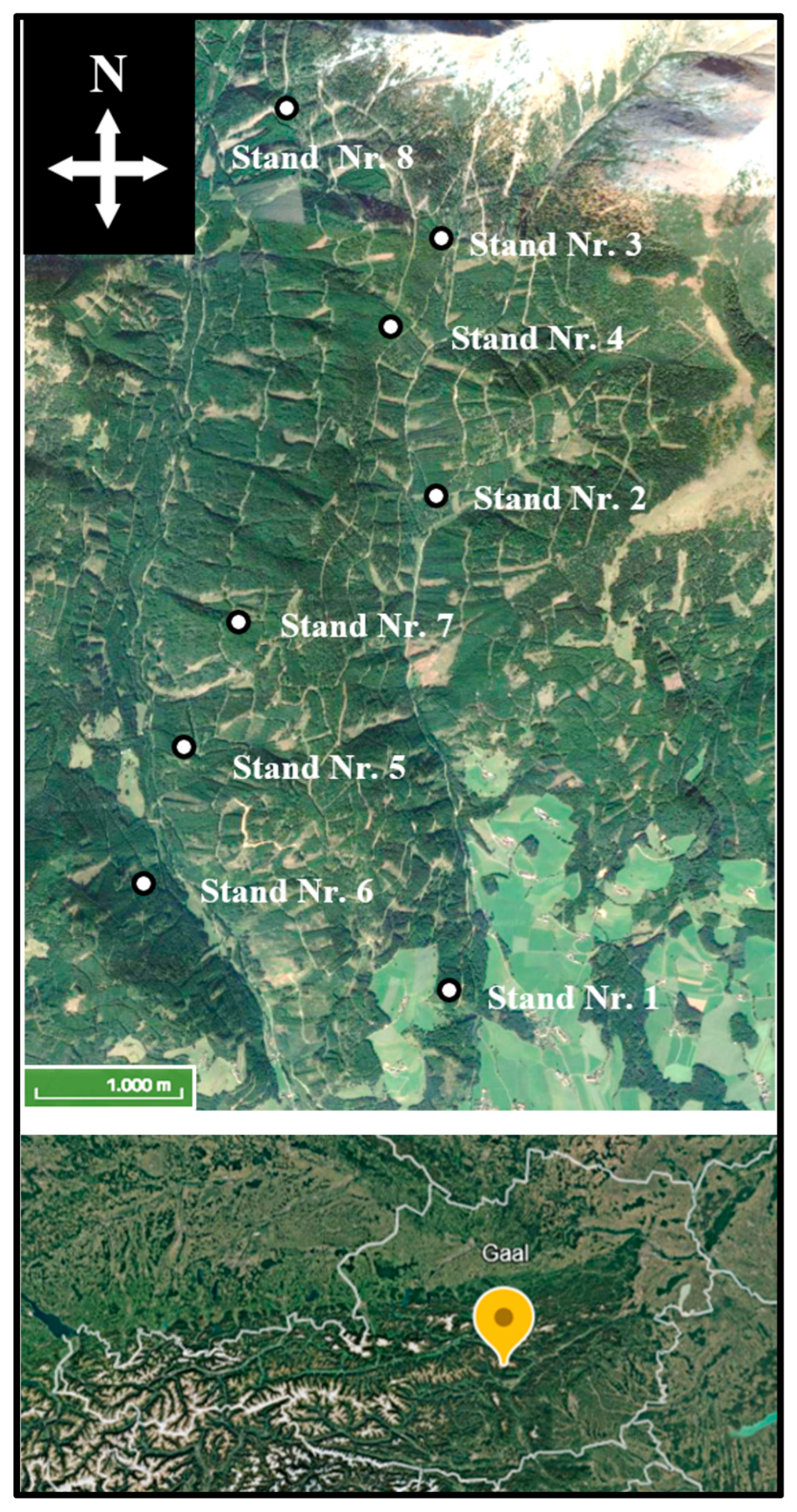
Figure 1. Location of the eight stands in the forest company “Wasserberg” in Gaal/Austria.
Forests 16 00890 g001
Figure 2. Graphical overview of the calculation steps in this paper.
Forests 16 00890 g002
Figure 3. Standard error [%] of total bark stripping damage (1st column), summer bark stripping damage (2nd column) and new bark stripping damage (3rd column) obtained using the Hansen–Hurwitz (HH) and the Horvitz–Thompson (HT) estimator as a function of the pre-defined grid space [m] for different initial sample sizes (n1 = 2 to 6 points per stand).
Forests 16 00890 g003
Figure 4. Inclusion probability for the possible sample points (grid cells in the stands) as a function of the chosen sampling scenario (grid space [m] and size of the initial sample n1) and for different damage.
Forests 16 00890 g004
Figure 5. Mean Standard Error [%] over all stands of the systematic sampling scheme depending on the inclusion probability and the plot radius [m] for the volume of damaged trees for different damage types (TOTAL = total damage; SUMMER = summer damage; NEW = new damage). Dashed line = SE of 10%.
Forests 16 00890 g005
Table 1. Biometric information and damage rates of the eight stands were obtained from a full census. The data include the following parameters: Area (the area of the stand), N (stem number per hectare), BA (basal area per hectare), and V (total volume per hectare). The damage rates are categorised as follows: TOTAL (overall percentage of trees with bark stripping damage), NEW (percentage of new bark stripping damage), and SUMMER (percentage of summer bark stripping damage).
StandArea
[ha]
N
[ha−1]
BA
[m2·ha−1]
V
[m3·ha−1]
Damage Percentage
[% of Volume]
TOTALNEWSUMMER
10.6593063.573156.20.2---
20.31119552.348913.4------
30.85104139.032911.10.3---
41.26150741.836233.90.90.5
50.54111638.642328.20.22.5
61.7749534.739313.80.23.4
71.22137039.231817.80.56.9
81.3986445.741315.90.24.9
TOTAL7.99101542.240722.10.42.9
Disclaimer/Publisher’s Note: The statements, opinions and data contained in all publications are solely those of the individual author(s) and contributor(s) and not of MDPI and/or the editor(s). MDPI and/or the editor(s) disclaim responsibility for any injury to people or property resulting from any ideas, methods, instructions or products referred to in the content.