Estimation of Tree Species Diversity in Warm Temperate Forests via GEDI and GF-1 Imagery

Abstract

Estimates of tree species diversity via traditional optical remote sensing are based only on the spectral variation hypothesis (SVH); however, this approach does not account for the vertical structure of a forest. The relative height (RH) indices derived from GEDI spaceborne LiDAR provide vertical vegetation structure information through waveform decomposition. Although RH indices have been widely studied, the optimal RH index for tree species diversity estimation remains unclear. This study integrated GF-1 optical imagery and GEDI LiDAR data to estimate tree species diversity in a warm temperate forest. First, random forest plus residual kriging (RFRK) was employed to achieve wall-to-wall mapping of the GEDI-derived indices. Second, recursive feature elimination (RFE) was applied to select relevant spectral and LiDAR features. The random forest (RF), support vector machine (SVM), and k-nearest neighbor (kNN) methods were subsequently applied to estimate tree species diversity through remote sensing data. The results indicated that multisource data achieved greater accuracy in tree species diversity estimation (average R² = 0.675, average RMSE = 0.750) than single-source data (average R² = 0.636, average RMSE = 0.754). Among the three machine learning methods, the RF model (R² = 0.760, RMSE = 2.090, MAE = 1.624) was significantly more accurate than the SVM (R² = 0.571, RMSE = 2.556, MAE = 1.995) and kNN (R² = 0.715, RMSE = 2.084, MAE = 1.555) models. Moreover, mean_mNDVI, mean_RDVI, and mean_Blue were identified as the most important spectral features, whereas RH30 and RH98 were crucial features derived from LiDAR for establishing models of tree species diversity. Spatially, tree species diversity was high in the west and low in the east in the study area. This study highlights the potential of integrating optical imagery and spaceborne LiDAR for tree species diversity modeling and emphasizes that low RH indices are most indicative of middle- to lower-canopy tree species diversity.

1. Introduction

Tree species diversity refers to the number of tree species and their relative abundance within a specific ecosystem, influencing forest structure and function [1,2]. Additionally, the taxonomic and ecological characteristics of forest sites often shape animal population composition, ultimately impacting global environmental integrity and biodiversity [3,4]. Tree species diversity is a key parameter for characterizing forest ecosystems, as trees support essential ecosystem services, such as nutrient cycling and water conservation; additionally, this index is useful for biomass estimation [5]. However, climate change has altered the distribution of vegetation and species [6,7], significantly impacting ecosystems worldwide [8,9]. Additionally, human activities have placed thousands of species at risk, driving many toward endangerment [1]. In forests, these changes have led to shifts in species diversity, disrupting ecological balance and long-term sustainability [1,10]. Therefore, there is an urgent need to develop effective methods for mapping the distribution of forest tree species diversity across large areas to assess their population carrying capacity.

Owing to its advantages of noncontact observation and large-scale continuous monitoring, remote sensing technology has provided a powerful technical support for monitoring tree species diversity [11,12,13]. Remote sensing methods for estimating biodiversity included direct and indirect approaches. In the direct approach, individual organisms or communities are identified through image classification algorithms [14,15]. For example, Tian et al. [16] employed the CART algorithm to classify mangroves using hyperspectral and LiDAR data and developed a biodiversity index system to assess mangrove species diversity in the study area. Similarly, Zhao et al. [17] applied a watershed segmentation algorithm to delineate individual tree crowns and combined seven vegetation indices with tree height to estimate species diversity in subtropical forests. The indirect approach is to combine environmental variables from remote sensing images with field observations in order to construct predictive models [18]. Mashiane et al. [19] assessed grassland species richness and diversity by extracting the NIR, the soil-adjusted vegetation index (SAVI), and the enhanced vegetation index (EVI) from Landsat 8 and Sentinel-2 imagery. Liu et al. [20] used multi-temporal Sentinel-2 imagery to evaluate tree species diversity in subtropical forests and found that images taken during transitional seasons (e.g., early spring and late autumn) yielded better predictive performance than those captured during the growing season. In addition, the accuracy of tree species richness estimation with remote sensing is influenced by mycorrhizal symbiosis types in forest ecosystems [21].

Although optical imagery has been used widely for its spatial continuity [22], forest vertical structure cannot be assessed using this method. To overcome this limitation, LiDAR technology has been increasingly integrated with optical remote sensing for improve tree species diversity estimation. Kamoske et al. [23] reported that spectral diversity, canopy structural heterogeneity, and topography collectively explain substantial biodiversity variability at the plot level. Ming et al. [24] further confirmed that combining LiDAR with spectral data enhances tree species diversity estimation, particularly in complex forest stands.

Among LiDAR-based data sources, the global ecosystem dynamics investigation (GEDI) spaceborne LiDAR system provides unprecedented high-resolution data on forest vertical stratification [25]. The GEDI has been widely used for biodiversity assessments [26], canopy height estimation [27], biomass measurement [28], vegetation growth monitoring [29], leaf area index calculation [30], and understory terrain characterization [31]. The relative height (RH) metrics derived from real and simulated LiDAR waveform data are among the most widely used metrics for characterizing the vertical structure of forests [26,32]. RH metrics quantify height above ground based on the distribution of backscattered energy (%) from different forest strata, allowing for characterization of vertical and horizontal structural complexity within 25 m footprints. However, research gaps remain regarding the optimal RH metrics for tree species diversity estimation, as well as the response patterns and ecological mechanisms underlying these relationships. Therefore, this study selected RH metrics at 10% height increments to represent the complex vertical structure of forest stands and explore their contributions to tree species diversity modeling and their ecological significance. While GEDI enables high sampling density, it does not provide wall-to-wall forest parameter observations, so combining GEDI with optical imaging has become a research trend. GF-1 imagery, with its high spatial resolution and rich spectral and texture information, has been widely used in studies of crop monitoring [33], forest structure monitoring [34], and land use classification [35].

In recent years, machine learning algorithms have been extensively used in the monitoring and mapping of forest tree species diversity [36,37,38,39]. Commonly applied algorithms include the random forest (RF) [40], support vector machine (SVM) [41], and k-nearest neighbors (kNN) [42] methods. As an extension of traditional decision trees, RF enhances predictive accuracy by integrating multiple decision trees and assessing feature importance through accuracy reductions when a feature is removed [43]. An SVM projects data from a low-dimensional space to a higher-dimensional space by selecting appropriate kernel functions. This transformation helps address the issue of linear inseparability between data points, reducing structural risk and effectively handling nonlinear data [44]. Additionally, SVMs are known for their strong generalization capabilities, particularly when dealing with high-dimensional datasets [45]. A kNN yields the weighted average of parameter values from the k nearest neighbor plots on the basis of the spectral distance between the sample pixel and the estimated pixel. The closer the sample pixel is to the estimated pixel, the higher the weight it receives [46]. In this study, we integrated RF, SVM, and kNN algorithms with remote sensing-derived spectral, textural, and structural metrics from GEDI and GF-1 to construct predictive models for tree species diversity estimation.

The Taihang Mountains serve as a geographical boundary between the north China plain and the loess plateau, acting as a critical ecological barrier for the Beijing–Tianjin–Hebei economic zone [47]. Historically, extensive deforestation in the southern Taihang Mountains for agriculture and timber resulted in the near-complete removal of natural forests, reducing forest cover to less than 5% [48]. This deforestation led to severe environmental degradation, including soil erosion, frequent droughts, and other significant ecological issues [49]. To address these challenges, China has implemented long-term ecological restoration projects, leading to the gradual recovery of vegetation in the Taihang Mountains [50]. Understanding tree species diversity in naturally regenerated secondary forests is essential for promoting vegetation restoration, conserving biodiversity, and assessing the ecological recovery process in this region. This study aimed to: (1) quantify the relationships between tree species diversity and variables derived from GF-1 and GEDI and identify the optimal RH metrics for tree species diversity modeling and their ecological implications; (2) explore effective methods for high-accuracy forest diversity mapping; and (3) develop tree species diversity maps via GEDI and GF-1 data to support forest diversity management.

2. Materials and Methods

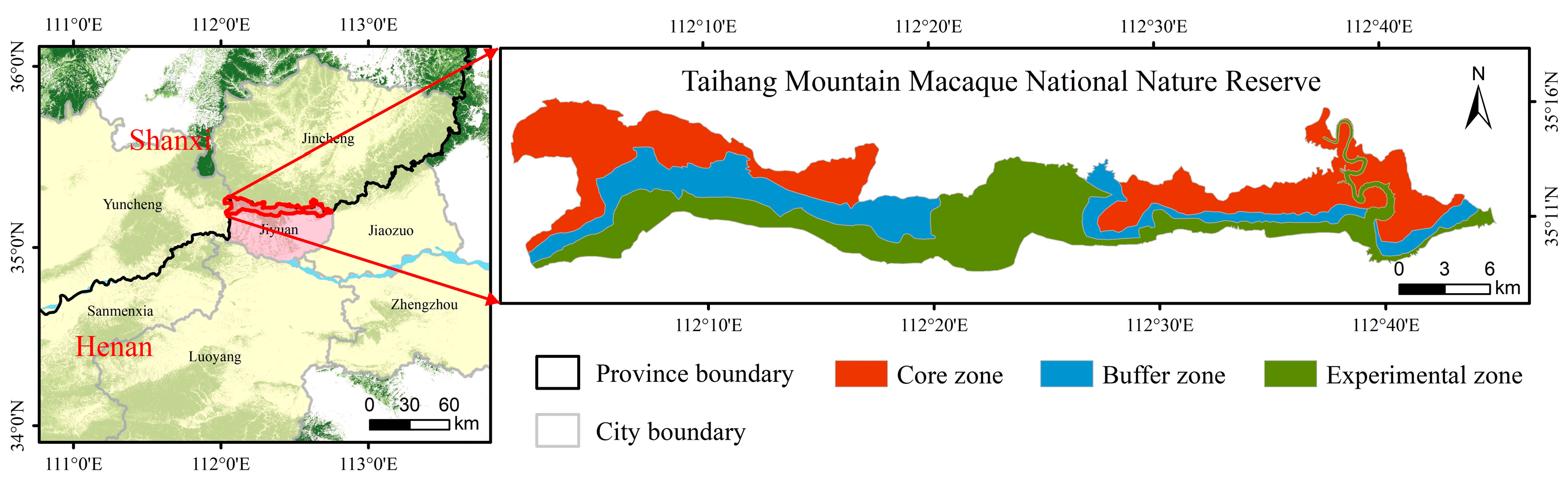
2.1. Study Area

The Taihang Mountains Macaque National Nature Reserve is located in northwestern Henan Province, China, on the southern slope of the Taihang Mountain (34°54′–35°16′ N, 112°02′–112°52′ E), covering approximately 15,572 hectares [51]. The functional zoning of the protected area is shown in Figure 1. The climate is classified as semihumid or semiarid continental monsoon. The annual average temperature is 14 °C [52], with an annual sunshine duration of 1727.6 h and an annual precipitation of 860 mm [53]. The region is predominantly hilly and mountainous, with soil types consisting mainly of brown and cinnamon soils, which are typically acidic or neutral [54]. The main vegetation species in the area include Quercus aliena var. acutiserrata, Quercus variabilis, Pistacia chinensis, and Carpinus turczaninovii [53,54,55], as shown in

Table 1. Descriptive statistics for the DBH and tree height of the main tree species in the study area.

Scientific Name	Leaf Type	DBH			Tree Height
		Min	Max	Mean	Min	Max	Mean
Quercus variabilis	broad	5	74	15.75	2	33	10.6
Quercus aliena	broad	5	84	19.85	2	33	10.1
Pinus tabuliformis	needle	5	66	16.29	2	35.4	6.7
Carpinus turczaninovii	broad	5	79	8.90	2	26	5.8
Quercus baronii	broad	5	33	8.89	2.5	16	7.7
Quercus aliena var. acuteserrata	broad	5	31.4	12.16	2.2	15.5	8.5
Ulmus pumila	broad	5.2	79.6	15.16	3.5	23	12.1
Rhus potaninii	broad	5	26.7	12.13	2.1	17.5	6.2
Cotinus coggygria var. cinereus	broad	5	45	13.45	2.5	15.6	8.8
Castanea mollissima	broad	5	28	7.80	2.2	10.9	4.8
Malus spectabilis	broad	5.1	26.7	10.61	2.3	21.2	9.2
Carya cathayensis	broad	5	36	13.75	3	16	9.1
Robinia pseudoacacia	broad	5	25.2	10.40	2.4	9	5.2
Acer davidii	broad	5	37.6	12.85	2.5	27.2	8.7
Toxicodendron vernicifluum	broad	5	36.8	11.55	2	14.9	6.7
Pistacia chinensis	broad	5.2	41	18.12	3.7	20	11.8
Tilia chinensis	broad	5.1	28.3	10.66	2.1	18	7.4
Populus × canadensis	broad	5.1	24.5	10.41	3.1	10.2	6.1
Acer pictum subsp. mono	broad	5	31.5	11.64	2.5	15.3	7.9
Diospyros lotus	broad	5	23.3	10.68	2	22.5	8.8
Swida macrophylla	broad	5	23.3	10.68	2	22.5	8.8

.

2.2. Field Investigation of Sample Plots

Between June to September 2020, 10 permanent forest plots, each covering an area of 100 m × 100 m, were established in the Taihang Mountains Macaque National Nature Reserve following the large-scale forest plot methodology outlined by Condit [56]. Each plot was subdivided into 25 subplots of 20 m × 20 m using a total station, resulting in a total of 250 subplots. Tree species with a diameter at breast height (DBH) ≥5 cm were surveyed, and the species name, coordinates, DBH, and tree height for each individual tree were recorded. In addition, within the framework of the Ninth National Forest Continuous Inventory, 14 plots measuring 28.8 m × 28.8 m were included. The measurements of and statistical data for the sample plots, grouped by vegetation zones, are presented in

Table 2. Statistics on plot measurements grouped by vegetation zones.

	Deciduous Broadleaf Forest	Evergreen Broadleaf Forest	Needleleaf-Broadleaf Mixed Forest	Needleleaf Forest	Waters	Building Land	Plow Land
Number of sample plots	165	44	30	25	18	13	5

. The study area is covered primarily by secondary deciduous broadleaf forests [54], which exhibit a wide natural distribution. Given the significant seasonal variations affecting deciduous broadleaf forests, a greater number of sample plots were established to capture their spectral characteristics and structural variability. The study area has experienced severe soil erosion and includes rocky mountainous regions. Although vegetation is gradually recovering, some exposed or sparsely vegetated patches remain [57]. To address this issue, approximately 10% of the sample plots were allocated to nonforest patches. These nonforest samples were included to: (1) provide negative constraints to prevent erroneous tree species composition predictions in complex regions, and (2) avoid dilution of forest diversity signals. The specific distribution of the sample plots is shown in Figure 2.

2.3. Tree Species Diversity Indices

To estimate tree species diversity based on field data, we used four different indicators: the Shannon index (H) [58], Simpson index (D) [59], Pielou index (J) [60], and species richness index (S) [61]. These indices were employed to quantify the diversity of tree species in the study area. In monitoring forest tree species diversity, S is typically determined based on the number of tree species within the study sample. The H index is the most commonly used measure of forest species diversity, as it reflects both species richness and the evenness of the species distribution within a community. The D index is also commonly employed to assess species diversity. It encompasses both the abundance and the number of species in an area and reflects the probability that two randomly selected individuals will belong to the same species. The formulas for calculating these diversity indices are as follows:

$$H=-{\displaystyle \sum _{i=1}^N{P}_i\ln P_i}$$

(1)

$$D=1-{\displaystyle \sum _{i=1}^N{P}_i^2}$$

(2)

$$J=-{\displaystyle \frac{1}{\ln N}}{\displaystyle \sum _{i=1}^N{P}_i\ln P_i}$$

(3)

$$S=N$$

(4)

N is the number of tree species in the plot. The proportion of the individual number of P_i tree species i relative to the total number of tree species is measured.

According to Formulas (1)–(4), the tree species diversity index in 300 plots was calculated, and the results for each index were summarized. The results are shown in

Table 3. Descriptive statistical characteristics of tree species diversity.

Diversity Index	Min	Max	Mean	Median	Standard Deviation	Coefficient of Variation	Kurtosis	Skewness
H	0.00	2.40	1.01	1.06	0.64	63.22	−1.07	−0.12
D	0.00	0.89	0.47	0.54	0.28	58.16	−1.06	−0.51
J	0.00	0.99	0.55	0.64	0.27	49.78	−0.31	−0.92
S	0.00	16.00	6.01	6.00	4.07	67.71	−0.65	0.35

.

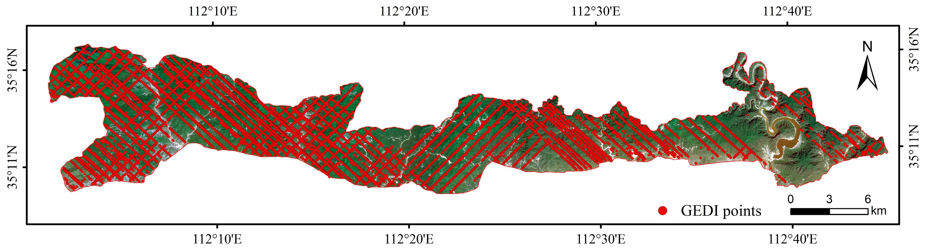
2.4. GEDI Data and Preprocessing

In addition, since April 2019, NASA’s GEDI LiDAR sensor aboard the International Space Station has been collecting footprint data over an average span of 25 m. The GEDI data used in this study were obtained from the NASA Land Processes Distributed Active Archive Center (https://search.earthdata.nasa.gov/search (accessed on 15 April 2024)). The orbits and laser footprints in the study area from 2019 to 2022 were extracted for analysis.

The RH index was derived from the cumulative distribution function of the GEDI waveform, which is centered on the ground echo height at time 0. As such, the RH value represents the height at which the GEDI waveform energy is received, ranging from 0% to 100% in 1% increments [62]. Importantly, the RH index can be negative in cases of wide ground signals or sparse vegetation [63]. The RH index reflects the complexity of a stand’s vertical structure. According to the height variation hypothesis (HVH) [64], large changes in tree height indicate a complex forest structure and high tree species diversity. In this study, a 10% increment was used to select RH values in the range of 10 to 90 to explore the potential of the RH index for representing the complex stand vertical structure relationship. Considering that RH100 exhibits significant noise, RH98 was chosen as a substitute. The plant area index (PAI) represents the vegetation area per unit surface area. It plays a crucial role in regulating photosynthesis and plant respiration and is an important variable for modeling vegetation productivity, carbon exchange, and climate systems. As a canopy density indicator, the PAI is useful for monitoring forest health and conditions [65]. Foliage height diversity (FHD) is related to the Shannon entropy of the vertical leaf profile [66], which represents the vertical stratification and canopy complexity of a forest. The FHD is an important indicator for assessing diverse habitats in the forest canopy with rich animal and plant species [67]. The total canopy cover (TCC) is the percentage of the vertical projection of canopy material covering the ground, providing a broad and spatially continuous measure of surface vegetation coverage dynamics [68]. The aboveground biomass density (AGBD) is essential for studying the carbon cycle, biodiversity, and climate change [69]. In this study, Python 3.9 was used to extract and process 14 parameter indicators from the L2A, L2B, and L4A products (as shown in

Table 4. Description of the GEDI parameters.

Data	Variables	Description
L2A	RH10, RH20, RH30, RH40, RH50, RH60, RH70, RH80, RH90, RH98	Based on a 10% increment in the relative height index, RH100 exhibited significant noise and was replaced by RH98
L2B	PAI	Plant area index
	FHD	Foliage height diversity index
	TCC	Total canopy cover
L4A	AGBD	Aboveground biomass density (Mg/ha)

).

First, the L2A product parameter shot_number was extracted to create the spot number index. The lon_lowestmod and lat_lowestmod parameters were subsequently used to obtain the longitude and latitude information of the laser footprints. Only footprints within the study area were retained, resulting in a total of 69,835 laser footprints. Next, parameters from the L2B and L4A products were extracted using the shot_number field in the L2A dataset. After five screening criteria were applied (as shown in

Table 5. GEDI effective spot screening conditions.

Parameter	Condition	Description
quality_flag	1	Indicates that the waveform meets specific criteria based on energy, sensitivity, amplitude, and real-time surface tracking quality and can be expressed as a valid waveform.
rx_assess_flag	0	Flags indicating various error conditions possible in rxwaveform.
degrade_flag	0	The state degradation sign is ‘1’, indicating that the state of the indicated direction or positioning information decreases, which affects the accuracy of the data.
sensitivity	≥0.90	Considering the signal-to-noise ratio of the waveform, the maximum canopy coverage that can be penetrated is indicated.
ǀelev_lowestmode—SRTMǀ	≤50	Because GEDI is susceptible to clouds in data acquisition, the removal of elev_lowestmode and the SRTM of GEDI footprints have increased differences in spots.

), a total of 12,055 valid laser footprints were selected. The distribution of the GEDI laser footprints is shown in Figure 3.

2.5. GF-1 Data and Preprocessing

GF-1, the first satellite launched as part of the China High Resolution Earth Observation System, was deployed on 26 April 2013. The satellite is equipped with two primary types of sensors: the panchromatic and multispectral sensor (PMS) and four wide-field-of-view (WFV) sensors (GF-1 satellite was developed by China Aerospace Science and Technology Corporation (CASC), located in Beijing, China.). The GF-1 satellite combines high spatial, temporal, and multispectral resolution capabilities, making it a powerful tool for optical remote sensing. The PMS sensor captures panchromatic images with a resolution of 2 m and multispectral images with a resolution of 8 m, covering four bands. The specific parameters are shown in

Table 6. GF-1 image parameters.

Type	Waveband	Wavelength Coverage	Spatial Resolution
Panchromatic	PAN	0.45–0.90	2 m
Multispectral	Blue	0.45–0.52	8 m
	Green	0.52–0.59	8 m
	Red	0.63–0.69	8 m
	NIR	0.77–0.89	8 m

. In this study, a 2 m resolution panchromatic image and an 8 m resolution multispectral image of the study area were obtained in May 2020. These images were used to quantify the spectral variation characteristics of the forest tree species. The images were preprocessed on the ENVI 5.6 (Harris Geospatial Solutions, located in Loveland, CO, USA) software platform, which involved radiometric calibration, atmospheric correction, mosaic splicing, and image cropping. As a result, a 2 m spatial resolution panchromatic image and multiband surface reflectance data with an 8 m spatial resolution for the study area were generated.

On the basis of the spectral variation hypothesis (SVH) and its relationship with tree species diversity, various spectral feature variables, such as the B1–B4 multispectral bands, the B5 panchromatic band, 18 vegetation indices (

Table 7. Vegetation index extraction based on GF-1 data.

Vegetation Indices	Expression	References
Normalized difference vegetation index (NDVI)	$\mathrm{N}\mathrm{D}\mathrm{V}\mathrm{I}=(\mathrm{N}\mathrm{I}\mathrm{R}-\mathrm{Re}\mathrm{d})/(\mathrm{N}\mathrm{I}\mathrm{R}+\mathrm{Re}\mathrm{d})$	[71]
Carotenoid reflectance index (CRI)	$\mathrm{C}\mathrm{R}\mathrm{I}=1/\mathrm{B}\mathrm{l}\mathrm{u}\mathrm{e}-1/\mathrm{G}\mathrm{r}\mathrm{e}\mathrm{e}\mathrm{n}$	[72]
Enhanced vegetation index (EVI)	$\mathrm{E}\mathrm{V}\mathrm{I}=2.5\ast (\mathrm{N}\mathrm{I}\mathrm{R}-\mathrm{Re}\mathrm{d})/(\mathrm{N}\mathrm{I}\mathrm{R}+6\ast \mathrm{Re}\mathrm{d}-7.5\ast \mathrm{B}\mathrm{l}\mathrm{u}\mathrm{e}+1)$	[73]
Differential vegetation index (DVI)	$\mathrm{D}\mathrm{V}\mathrm{I}=\mathrm{N}\mathrm{I}\mathrm{R}-\mathrm{Re}\mathrm{d}$	[74]
Nonlinear vegetation index (NIL)	$\mathrm{N}\mathrm{L}\mathrm{I}=(\mathrm{N}\mathrm{I}{\mathrm{R}}^2-\mathrm{Re}\mathrm{d})/(\mathrm{N}\mathrm{I}{\mathrm{R}}^2+\mathrm{Re}\mathrm{d})$	[71]
Modified normalized vegetation index (mNDVI)	$\mathrm{m}\mathrm{N}\mathrm{D}\mathrm{V}\mathrm{I}=(\mathrm{N}\mathrm{I}\mathrm{R}-\mathrm{Re}\mathrm{d})/(\mathrm{N}\mathrm{I}\mathrm{R}+\mathrm{Re}\mathrm{d}-2\ast \mathrm{B}\mathrm{l}\mathrm{u}\mathrm{e})$	[75]
Renormalized vegetation index (RDVI)	$\mathrm{R}\mathrm{D}\mathrm{V}\mathrm{I}=(\mathrm{N}\mathrm{I}\mathrm{R}-\mathrm{Re}\mathrm{d})/\sqrt{\mathrm{N}\mathrm{I}\mathrm{R}+\mathrm{Re}\mathrm{d}}$	[76]
Soil-adjusted vegetation index (SAVI)	$\mathrm{S}\mathrm{A}\mathrm{V}\mathrm{I}=1.5\ast (\mathrm{N}\mathrm{I}\mathrm{R}-\mathrm{Re}\mathrm{d})/(\mathrm{N}\mathrm{I}\mathrm{R}+\mathrm{Re}\mathrm{d}+0.5)$	[77]
Optimized soil-adjusted vegetation index (OSAVI)	$\mathrm{O}\mathrm{S}\mathrm{A}\mathrm{V}\mathrm{I}=(\mathrm{N}\mathrm{I}\mathrm{R}-\mathrm{Re}\mathrm{d})/(\mathrm{N}\mathrm{I}\mathrm{R}+\mathrm{Re}\mathrm{d}+0.16)$	[78]
Ratio vegetation index (RVI)	$\mathrm{R}\mathrm{V}\mathrm{I}=\mathrm{N}\mathrm{I}\mathrm{R}/\mathrm{Re}\mathrm{d}$	[79]
Green chlorophyll vegetation index (GCVI)	$\mathrm{G}\mathrm{C}\mathrm{V}\mathrm{I}=\mathrm{N}\mathrm{I}\mathrm{R}/\mathrm{G}\mathrm{r}\mathrm{e}\mathrm{e}\mathrm{n}-1$	[80]
Wide dynamic range vegetation index (WDRVI)	$\mathrm{W}\mathrm{D}\mathrm{R}\mathrm{V}\mathrm{I}=(0.1\ast \mathrm{N}\mathrm{I}\mathrm{R}-\mathrm{Re}\mathrm{d})/(0.1\ast \mathrm{N}\mathrm{I}\mathrm{R}+\mathrm{Re}\mathrm{d})$	[81]
Green wide dynamic range vegetation index (GWDRVI)	$\mathrm{G}\mathrm{W}\mathrm{D}\mathrm{R}\mathrm{V}\mathrm{I}=(0.1\ast \mathrm{N}\mathrm{I}\mathrm{R}-\mathrm{G}\mathrm{r}\mathrm{e}\mathrm{e}\mathrm{n})/(0.1\ast \mathrm{N}\mathrm{I}\mathrm{R}+\mathrm{G}\mathrm{r}\mathrm{e}\mathrm{e}\mathrm{n})$	[82]
Global environmental monitoring index (GEMI)	$\mathrm{G}\mathrm{E}\mathrm{M}\mathrm{I}=\mathrm{e}\mathrm{t}\mathrm{a}\ast (1-0.25\ast \mathrm{e}\mathrm{t}\mathrm{a})-(\mathrm{Re}\mathrm{d}-0.125)/(1-\mathrm{Re}\mathrm{d})$	[83]
	$\mathrm{e}\mathrm{t}\mathrm{a}=(2\ast (\mathrm{N}\mathrm{I}{\mathrm{R}}^2-\mathrm{Re}{\mathrm{d}}^2)+1.5\ast \mathrm{N}\mathrm{I}\mathrm{R}+0.5\ast \mathrm{Re}\mathrm{d})/(\mathrm{N}\mathrm{I}\mathrm{R}+\mathrm{Re}\mathrm{d}+0.5)$
Green difference vegetation index (GDVI)	$\mathrm{G}\mathrm{D}\mathrm{V}\mathrm{I}=\mathrm{N}\mathrm{I}\mathrm{R}-\mathrm{G}\mathrm{r}\mathrm{e}\mathrm{e}\mathrm{n}$	[84]
Green normalized difference vegetation index (GNDVI)	$\mathrm{G}\mathrm{N}\mathrm{D}\mathrm{V}\mathrm{I}=(\mathrm{N}\mathrm{I}\mathrm{R}-\mathrm{G}\mathrm{r}\mathrm{e}\mathrm{e}\mathrm{n})/(\mathrm{N}\mathrm{I}\mathrm{R}+\mathrm{G}\mathrm{r}\mathrm{e}\mathrm{e}\mathrm{n})$	[85]
Green ratio vegetation index (GRVI)	$\mathrm{G}\mathrm{R}\mathrm{V}\mathrm{I}=\mathrm{N}\mathrm{I}\mathrm{R}/\mathrm{G}\mathrm{r}\mathrm{e}\mathrm{e}\mathrm{n}$	[84]
Red green ratio index (RGRI)	$\mathrm{R}\mathrm{G}\mathrm{R}\mathrm{I}=\mathrm{Re}\mathrm{d}/\mathrm{G}\mathrm{r}\mathrm{e}\mathrm{e}\mathrm{n}$	[86]

), and the first principal component of the multispectral data, were extracted from the preprocessed GF-1 images. Following Liu et al. [70], gray-level co-occurrence matrices were established for the multispectral bands (3 × 3 window size) and the panchromatic band (7 × 7 window size), resulting in 16 texture features (

Table 8. GLCM texture feature variables and their formulas.

GLMC
$\mathrm{Mean}={\displaystyle {\sum }_{i,j=0}^{N-1}i{P}_{i,j}}$	$\mathrm{Dissimilarity}={\displaystyle {\sum }_{i,j=0}^{N-1}{P}_{i,j}\left|i-j\right|}$
$\mathrm{Variance}={{\displaystyle {\sum }_{i,j=0}^{N-1}{P}_{i,j}(i-\mathrm{Mean})}}^2$	$\mathrm{Entropy}={\displaystyle {\sum }_{i,j=0}^{N-1}{P}_{i,j}}\ln P_{i,j}$
$\mathrm{Homogeneity}={{\displaystyle {\sum }_{i,j=0}^{N-1}{P}_{i,j}/(1+(i-j)}}^2)$	$\mathrm{Second} \mathrm{Moment}={\displaystyle {\sum }_{i,j=0}^{N-1}{P}_{i,j}^2}$
$\mathrm{Contrast}={{\displaystyle {\sum }_{i,j=0}^{N-1}{P}_{i,j}(i-j)}}^2$	$\mathrm{Correlation}={\displaystyle {\sum }_{i,j=0}^{N-1}{P}_{i,j}^2}(i-\mathrm{Mean})(j-\mathrm{Mean})/\mathrm{Variance}$

Note: For convenience of representation, the GLCM texture features are abbreviated as follows: mean (Mean), variance (Var), homogeneity (Homo), contrast (Cont), dissimilarity (Diss), entropy (Entr), second moment (SM), and correlation (Corr).

).

Using the SVH and the habitat heterogeneity hypothesis, the mean, standard deviation (std), variance (var), and coefficient of variation (cv) of the 40 optical remote sensing feature variables were calculated at a scale of 20 × 20 m to quantify the spatial heterogeneity of the forest canopy spectral characteristics. To reduce model redundancy and minimize the impact of feature correlation, features with a correlation coefficient R > 0.8 were removed, leaving 43 variables.

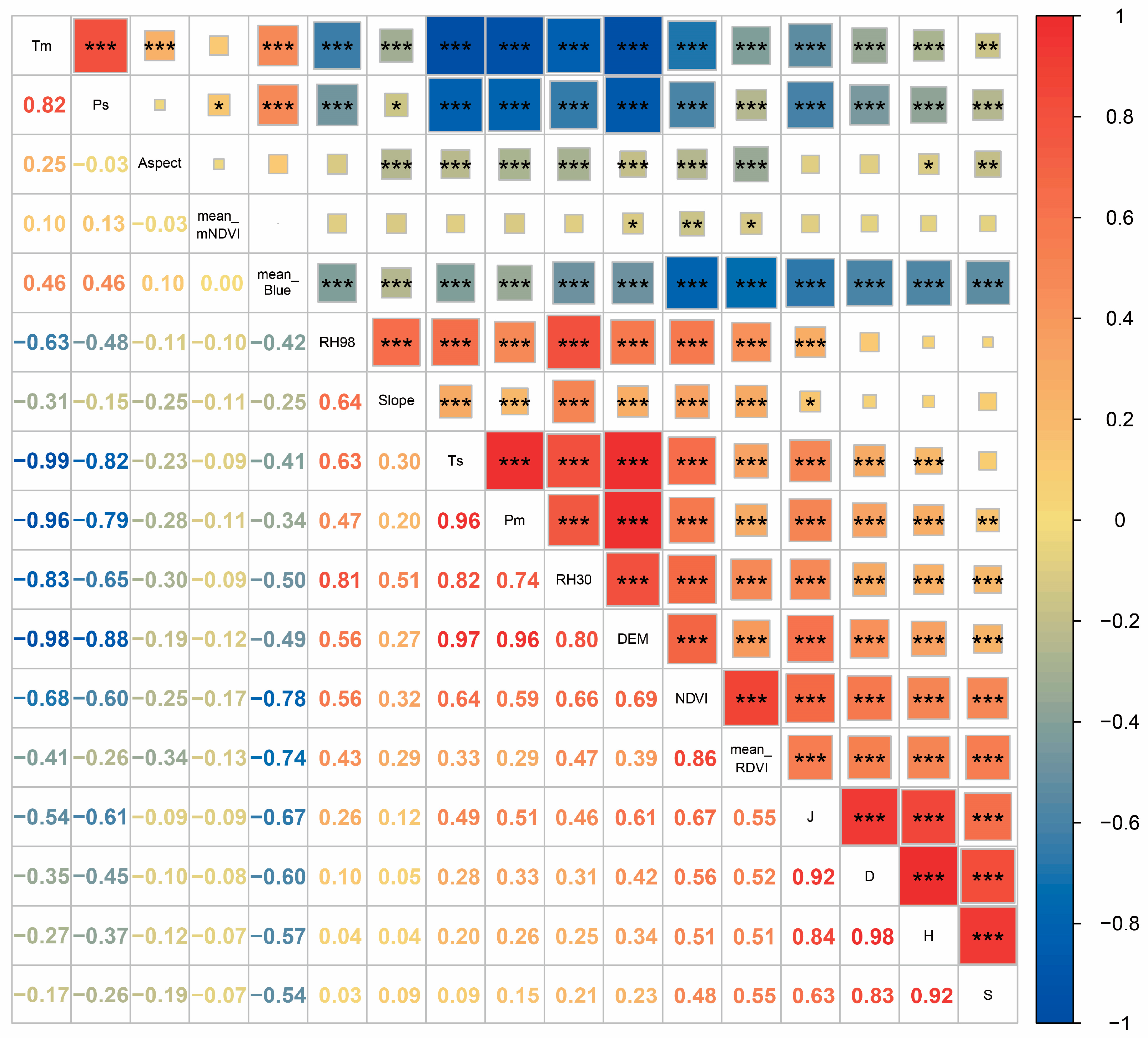
2.6. Remote Sensing Feature Selection

Recursive feature elimination (RFE) was proposed by Guyon in 2002 as a method for ranking features on the basis of some measure of their importance [87]. RFE starts with the entire feature set, and feature importance is iteratively evaluated. During each step, the least relevant feature is removed, and the importance of the remaining features is recalculated. This process continues until only one feature remains, allowing evaluation of all modeled variables from least to most important. The reverse order of feature elimination represents the feature importance ranking. In random forest regression, the RMSE is used as the evaluation metric to assess feature importance.

2.7. Modeling Method

2.7.1. Random Forest

Random forest (RF) [40] is a widely used supervised machine learning algorithm and ensemble learning method. An ensemble prediction is generated by aggregating the outputs of a set of randomly grown trees with the number of trees. In multiclass classification problems, the relative frequency of the terminal nodes for each class label in the random forest classification tree generates a predicted probability for each class. In regression problems, the average of the terminal node values is used to obtain the predicted value for the response variable, Y. Equivalently, the predicted value of the RF can be expressed as a weighted convex combination of the results from each individual tree. This property makes the RF a locally weighted average estimator. A unique feature of RF trees is their randomness, which manifests in the following ways: (a) each tree is built using independent bootstrap samples (i.e., samples are drawn with replacement from the original dataset, with the sample size n equal to the size of the original dataset); and (b) random feature selection occurs during tree growth. At each node, a random subset of 1 ≤ mtry ≤ p features is selected, where p is the total number of features. The variables from this subset that provide the best split are used to divide the data at that node. The process of recursively splitting the tree continues until one of two conditions is met: either the data at a node cannot be divided into groups with different outcomes, or the sample size at the node becomes too small. The terminal node size (at the leaf of the tree) is constrained by a minimum node size, where node_size ≥ 1, ensuring that each terminal node is associated with at least one unique case.

In the Python 3.9 environment, the model was trained by randomly selecting 70% of the data as the training set and the remaining 30% as the test set. All three machine learning methods utilized the GridSearchCV function from the sklearn 1.3.1 library for hyperparameter tuning, with the search range specified in

Table 9. The hyperparameter search ranges of the three machine learning algorithms.

Model	Parameters
RF	n_estimators = 50, 100, 150, 200, 300, 500, 1000
	max_feature = sqrt, log2, none
	max_depth = 1, 3, 5, 10, 20, 50, 100, 200, none
SVM	C = 0.1, 0.5, 1, 3, 5, 10
	epsilon = 0.01, 0.1, 1
	kernel = linear, poly, rbf, sigmoid, precomputed
kNN	N_neighbors = 1, 2, 3, 5, 7, 9, 11, 15, 20, 25, 30

. Tenfold cross-validation was applied to evaluate model performance and identify the hyperparameter combination that achieved the highest validation accuracy.

2.7.2. Support Vector Machines

A support vector machine (SVM), proposed by Cortes and Vapnik [41], is a powerful and robust tool for data classification. Its robustness stems from its ability to perform structural risk minimization and its capacity to solve both linear and nonlinear problems. SVM is a function estimation method that learns from training data and maps input features to unknown outputs. The SVM model consists of two components: the training model and the prediction model. In the training phase, the model learns the relationships between the input features and the corresponding tree species diversity. This learned relationship is then applied to the SVM prediction model to obtain the regression values for each input test sample.

2.7.3. K-Nearest Neighbors

K-nearest neighbors (kNN) [42] is a typical nonparametric method that performs univariate or multivariate prediction on the basis of the spatial similarity between observation points and prediction points. The kNN method has been applied to classify remote sensing data and has been gradually applied for forest parameter estimation in combination with remote sensing data and sample data. There is no requirement for distribution of the data. The following formula is used:

$$\widehat{Y_t}={\displaystyle \frac{{\displaystyle {\sum }_{i=1}^k{d}_{t,i}^{-1}}{Y}_i}{{\displaystyle {\sum }_{i=1}^k{d}_{t,i}^{-1}}}}$$

(5)

where Ŷ_t is the estimated value of the target point of the t pixel; Y_i is the ith reference pixel value within a certain spectral distance in the t-pixel multidimensional space; and d_t,i is the spectral distance between two points. The forest parameters and forest types at the reference point are known. For the target point, the k nearest sample sites 1, 2,⋯⋯, k in the spectral space are determined, where d_t,1 ≤ d_t,2 ≤⋯⋯≤ d_t,k. Since different objects are affected by their neighbors differently, the greater the similarity between pair of sample points, the smaller the spectral distance between them, and vice versa. kNN is essentially an inverse distance weighted average method commonly used for spatial interpolation.

2.7.4. Random Forest Plus Residual Kriging

To overcome the spatial discontinuity issue of GEDI data, researchers often use machine learning or spatial interpolation methods to map GEDI variables in a study area. For example, Potapov et al. [27] applied a per-pixel machine-learning algorithm, combining the RH95 index from GEDI with Landsat imagery to map the global forest canopy height. Ren et al. [26] utilized inverse distance weighting (IDW) interpolation to achieve wall-to-wall mapping of the FHD and PAI indices of GEDI. Machine learning methods can be used to explore the complex nonlinear relationships between GEDI parameters and environmental variables; however, they often overlook the influence of neighboring data on the spatial distribution [88]. Furthermore, optical remote sensing data often reach a saturation point when high-level variables are estimated [89]. To address these limitations, we used a random forest plus residual kriging (RFRK) model to map GEDI variables, applying ordinary kriging to the residuals of the RF model and incorporating a random process to reduce model bias [88].

To simulate and predict the GEDI variables, we utilized three auxiliary data sources: terrain features, climate features, and the maximum annual NDVI values (

Table 10. Auxiliary features of RFRK.

Features	Data Source	Resolution	Variables
Terrain features	SRTM DEM	30 m	DEM, slope, and aspect
Climate features	WorldClim version 2.1	1 km	Annual mean temperature (tm), temperature seasonality (ts), annual mean precipitation (pm), and precipitation seasonality (ps)
NDVI	Sentinel-2	10 m	NDVI maximum value composite for 2020

) [90]. Terrain features (e.g., DEM, slope, and aspect) were derived from the 30 m spatial resolution SRTM DEM. Climate features, such as annual mean temperature (tm), temperature seasonality (ts), annual precipitation (pm), and precipitation seasonality (ps), were extracted from the global monthly weather data of WorldClim version 2.1 [91] at a 1 km resolution for the period of 1970–2000. The method of Su et al. [92] was used to calculate these climate features. The NDVI product was obtained via the Google Earth Engine to synthesize the maximum NDVI values from all Sentinel-2 imagery in 2020.

To maintain consistency across all the data, we employed a bilinear interpolation method to resample all the features to a 20 m resolution. Owing to the potential strong striping effects on the GEDI interpolated variables at ground level, we established a 500 m grid to filter the footprints. One footprint was retained per grid cell, ensuring an even distribution of footprints across the study area, resulting in 1225 selected footprints after filtering. We chose 20% of the footprints for independent model validation, whereas the remaining 80% were used for modeling with the RFRK approach.

2.8. Precision Evaluation Indices

The coefficient of determination (R²), mean square error (MSE), root mean square error (RMSE), and mean absolute error (MAE) were used to evaluate the accuracy of the tree species diversity estimates. The following formulas were used to calculate R², RMSE, and MAE:

$$R^2=1-{\displaystyle \frac{{\displaystyle {\sum }_{i=1}^n{(y_i-x_i)}^2}}{{\displaystyle {\sum }_{i=1}^n{(y_i-\overline{y})}^2}}}$$

(6)

$$RMSE=\sqrt{{\displaystyle \frac{{\displaystyle {\sum }_{i=1}^n{(x_i-y_i)}^2}}{n}}}$$

(7)

$$MAE={\displaystyle \frac{{\displaystyle {\sum }_{i=1}^n\left|x_i-y_i\right|}}{n}}$$

(8)

where x_i and y_i are the estimated and measured values, respectively, $\overline{y}$ is the average value, and n is the number of samples.

3. Results

3.1. RFRK Interpolation

The modeling results are presented in

Table 11. Accuracy of the RFRK model.

Variable	R2	RMSE	MAE
RH10	0.351	2.181	1.556
RH20	0.396	2.685	1.971
RH30	0.429	3.039	2.235
RH40	0.460	3.285	2.433
RH50	0.481	3.526	2.609
RH60	0.481	3.749	2.801
RH70	0.476	3.989	2.961
RH80	0.499	4.122	3.006
RH90	0.519	4.375	3.158
RH98	0.503	4.928	3.582
PAI	0.407	1.117	0.866
FHD	0.547	0.224	0.163
TCC	0.451	0.180	0.136
AGBD	0.469	53.307	37.647

, where FHD, RH90, and RH98 presented higher accuracies than the other parameters did, with R² values exceeding 0.5, whereas RH10 presented the lowest accuracy, with an R² of only 0.351. Some interpolation results are shown in Figure 4.

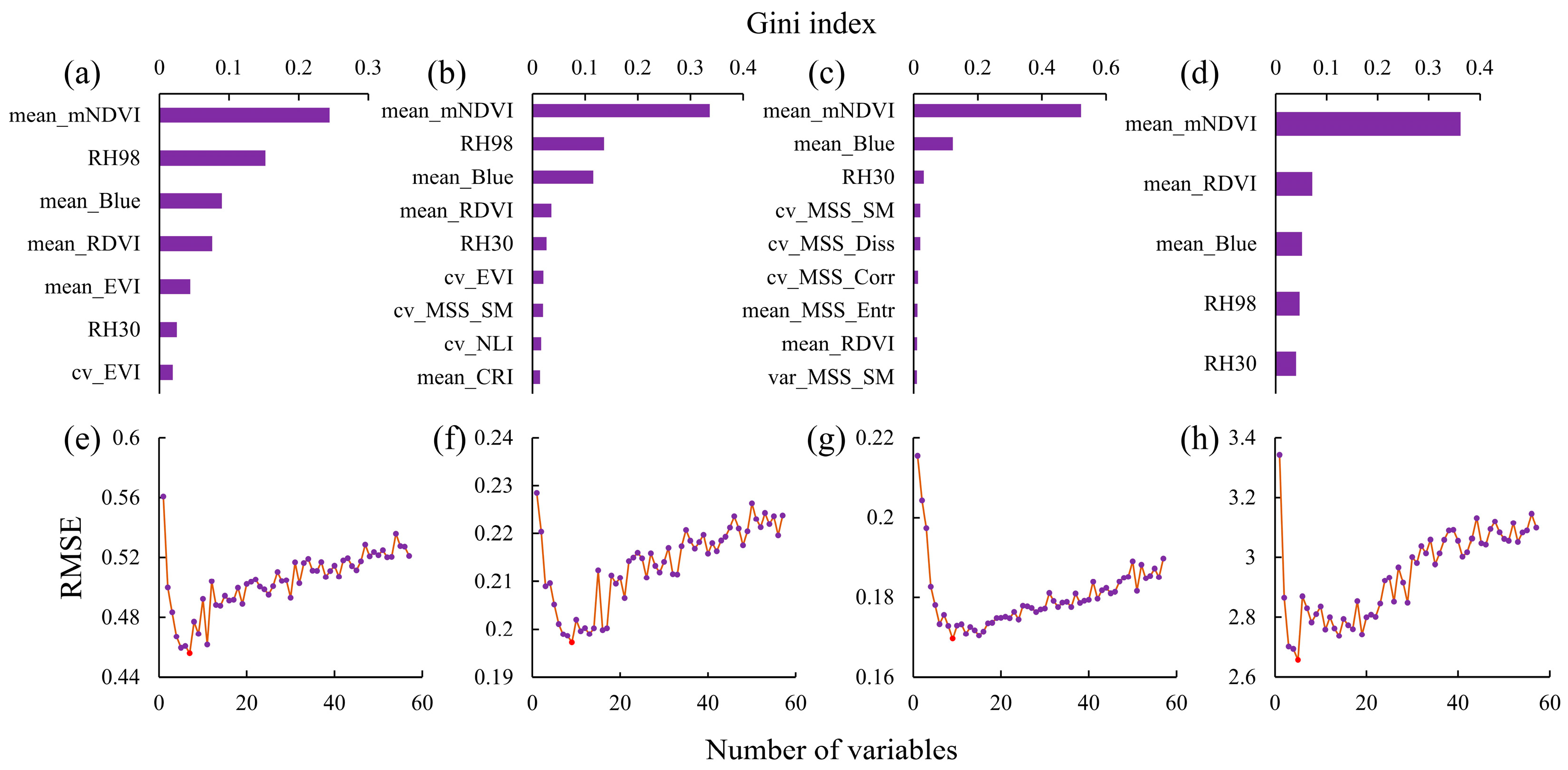
3.2. Feature Selection and Importance Ranking

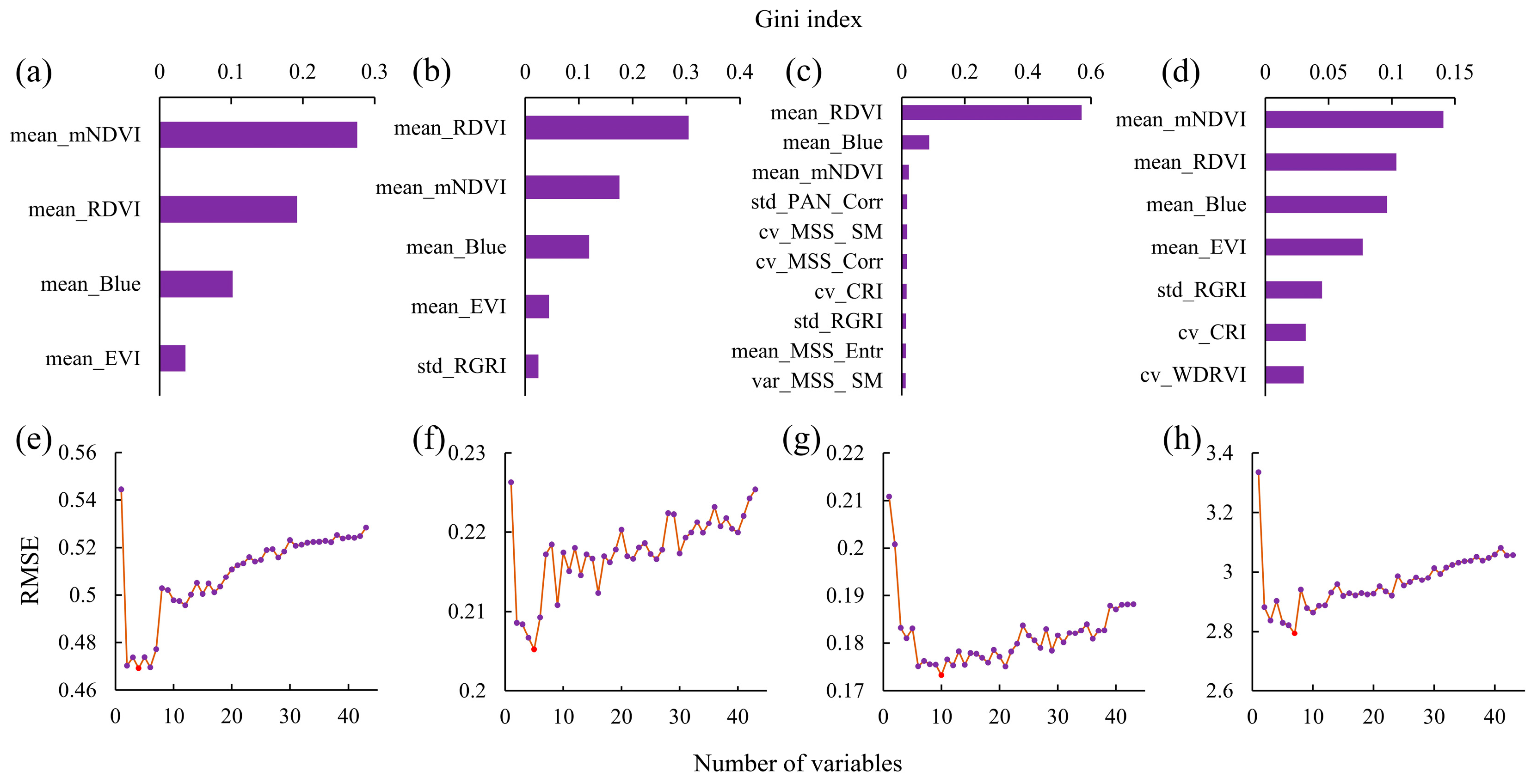
3.2.1. Spectral Feature Screening

The optimal numbers of features for the H index and the optimal set, including mean_mNDVI, mean_RDVI, mean_Blue, and mean_EVI, are shown in Figure 5. For the D index, the optimal set comprised mean_RDVI, mean_mNDVI, mean_Blue, mean_EVI, and std_RGRI. The J index requires 10 variables: mean_RDVI, mean_Blue, mean_mNDVI, std_PAN_Corr, cv_MSS_SM, cv_MSS_Corr, CV_CRI, std_RGRI, mean_MSS_Entr, and var_MSS_SM. For S, the optimal set included seven variables: mean_mNDVI, mean_RDVI, mean_Blue, mean_EVI, std_RGRI, CV_CRI, and cv_WDRVI.

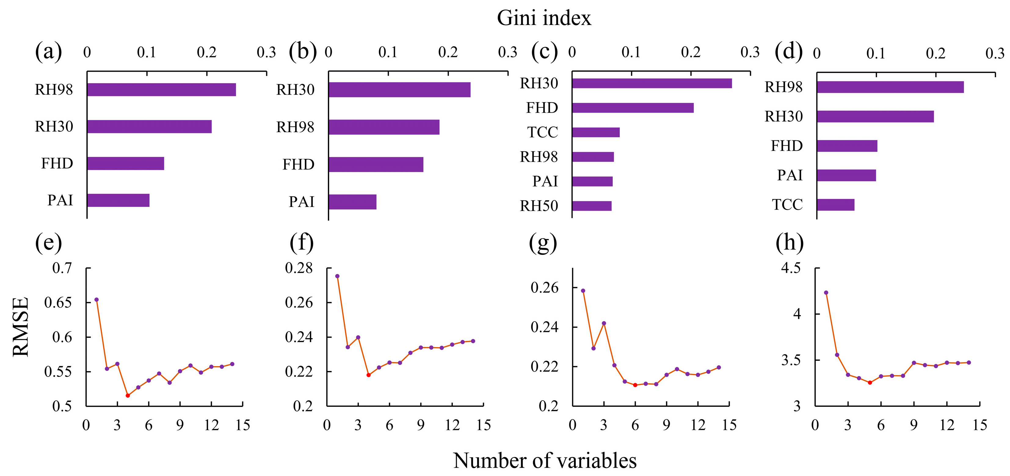
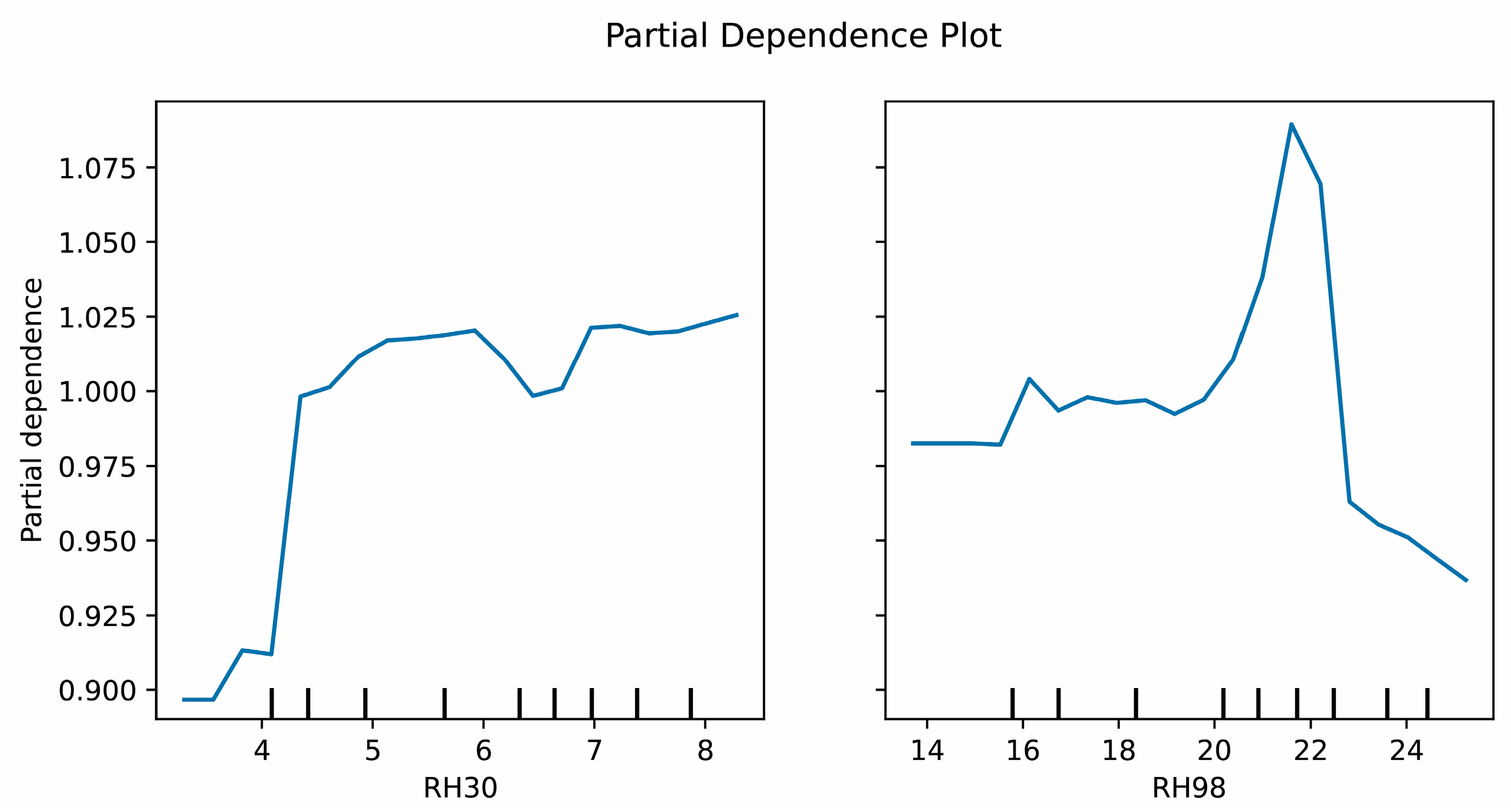
3.2.2. Vertical Structural Feature Screening

As shown in Figure 6, the optimal number of variables for the H index was four, comprising RH98, RH30, FHD and PAI. For the D index, the optimal number of variables was also four, comprising RH98, RH30, FHD, and PAI. For the J index, six variables were found to be optimal: RH30, FHD, TCC, RH98, PAI, and RH50. Finally, the optimal number of variables for the S index was five, and the selected variables were RH98, RH30, FHD, PAI, and TCC.

3.2.3. Fusion Feature Screening

For the combined remote sensing features, which integrate both spectral and vertical structural features, Figure 7 shows that the optimal numbers of features for the H index, D index, J index, and S index of tree species in the study area were seven, nine, nine, and five, respectively.

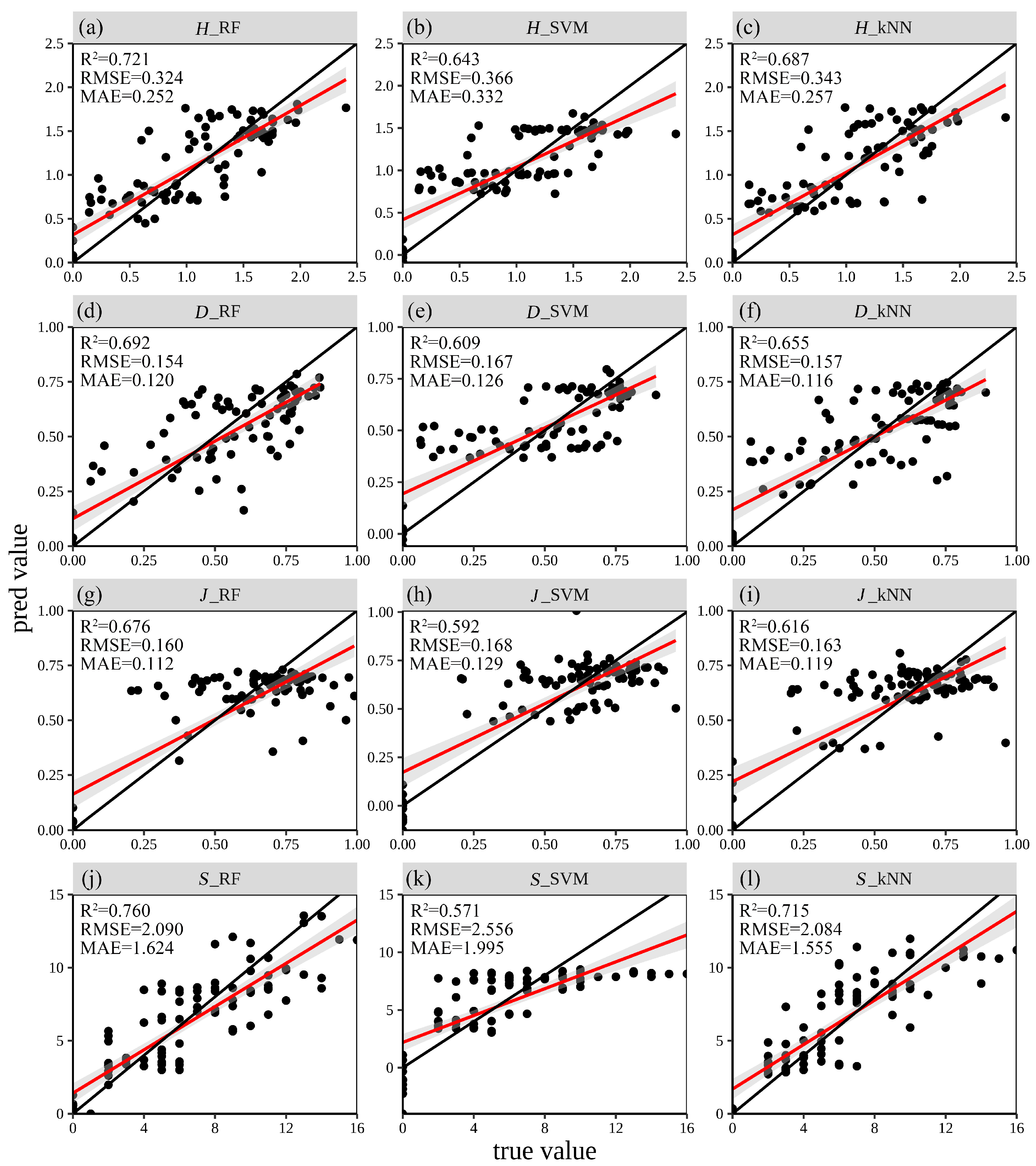
3.3. Estimation Accuracy

After feature selection, the RF, SVM, and kNN models were applied to estimate tree species diversity using GF-1 images, GEDI data, or GF-1 and GEDI fusion data. The results (

Table 12. The estimation accuracy of different data combinations for the four diversity indices.

Combined Variable		H		D		J		S		Average
		R2	RMSE	R2	RMSE	R2	RMSE	R2	RMSE	R2	RMSE
RF	GF-1	0.555	0.412	0.553	0.175	0.633	0.160	0.472	2.911	0.553	0.915
	GEDI	0.616	0.380	0.597	0.170	0.650	0.156	0.679	2.309	0.636	0.754
	GF-1 and GEDI	0.662	0.382	0.679	0.157	0.650	0.155	0.708	2.304	0.675	0.750
SVM	GF-1	0.342	0.501	0.393	0.204	0.505	0.196	0.323	3.296	0.391	1.049
	GEDI	0.573	0.401	0.547	0.192	0.386	0.420	0.506	2.741	0.503	0.939
	GF-1 and GEDI	0.446	0.456	0.578	0.180	0.518	0.195	0.623	2.618	0.541	0.862
kNN	GF-1	0.389	0.483	0.377	0.206	0.555	0.177	0.427	3.031	0.437	0.974
	GEDI	0.620	0.378	0.522	0.185	0.513	0.184	0.636	2.352	0.573	0.775
	GF-1 and GEDI	0.551	0.410	0.608	0.173	0.594	0.176	0.625	2.613	0.595	0.843

) showed that, for the same model, the mean R² values of the four indices predicted using the GF-1 and GEDI fusion data were higher than those predicted using either the GF-1 or the GEDI data alone. Additionally, the prediction accuracy of the approach with GEDI data was greater than that of the method with GF-1 imagery.

Specifically, for the RF model, the average R² values for GF-1 and GEDI increased from 0.553 and 0.636 to 0.675, whereas the average RMSE decreased from 0.915 and 0.754 to 0.750, respectively. For the SVM model, the average R² values for GF-1 and GEDI increased from 0.391 and 0.503 to 0.541, and the average RMSE decreased from 1.047 and 0.939 to 0.862, respectively. For kNN, the average R² values for GF-1 and GEDI increased from 0.437 and 0.573 to 0.595, respectively; however, the mean RMSE was still lower than that of GF-1 (0.974) and higher than that of GEDI (0.775). The RF model achieved the highest prediction accuracy for all the indices. Among the three data sources, the prediction accuracy for the H, D, J, and S indices was highest when the combined GF-1 and GEDI data were used, with R² values of 0.662, 0.679, 0.650, and 0.708, respectively.

Owing to the optimal feature set selected from the GF-1 and GEDI fusion data, and considering that the study area is characterized primarily by hills and mountains, terrain features, climate features, and the annual maximum NDVI (as shown in Table 12) were incorporated into the models. RF, SVM, and kNN models were then used to characterize the four diversity indices. The results (Figure 8) indicated that, after incorporating terrain and other features, the R² values for all the diversity index metrics of all the models were above 0.5. Except for the SVM prediction for the S index, all the other models showed varying degrees of improvement in terms of their ability to predict the four indices. Overall, the RF model exhibited the best fit, with the S index displaying the highest fit (R² = 0.76, RMSE = 2.09), followed by the D index (R² = 0.692, RMSE = 0.154), the J index (R² = 0.676, RMSE = 0.16), and the S index (R² = 0.721, RMSE = 0.324). The SVM model exhibited varying degrees of performance, with the best fit for the H index (R² = 0.643, RMSE = 0.336) and the lowest prediction accuracy for the S index (R² = 0.571, RMSE = 2.556). The kNN model demonstrated more stable fitting results than the SVM model did, with a good fit for the S index (R² = 0.715, RMSE = 2.084) and the poorest fit for the J index, still achieving an R² of 0.616 and an RMSE of 0.119. Across all the models, a common trend emerged: the low values of the indices tended to be slightly overestimated (above the 1:1 line), whereas the high values were underestimated (below the 1:1 line).

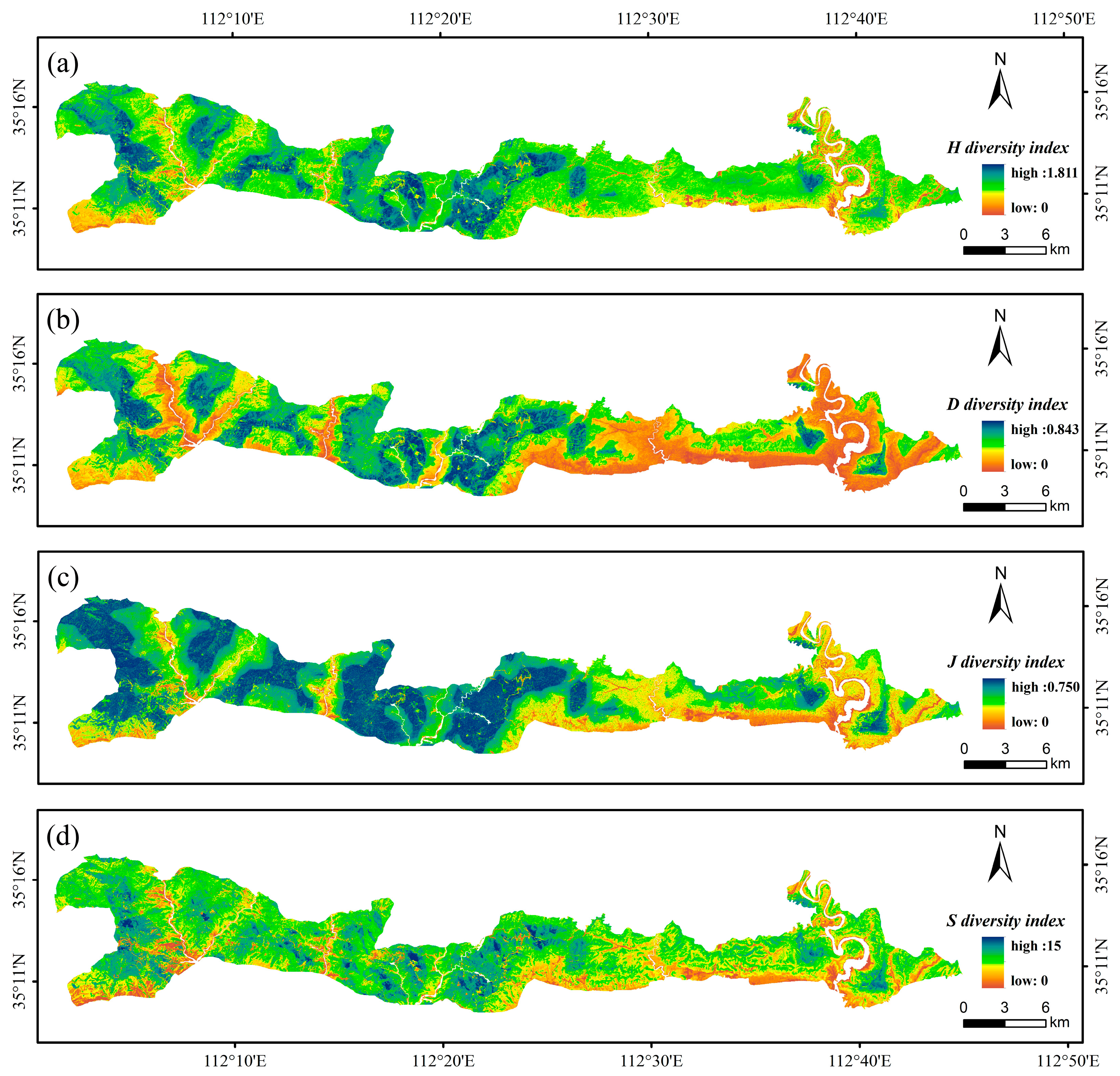
3.4. The Spatial Distribution of Tree Species Diversity

On the basis of the modeling results from the three machine learning models, the RF model was ultimately selected. Using the GF-1 and GEDI fusion features, terrain features, climate features, and annual maximum NDVI, the RF model was applied to map the H, D, J, and S indices of the tree species in the study area (Figure 9). The results indicate strong spatial heterogeneity in forest tree species diversity across the study area. Spatially, the prediction maps reveal notable consistency between the H index and the D index. The values of the four indices were predominantly distributed at moderate levels, with fewer values at both the lower and higher extremes. Overall, the diversity levels followed a spatial distribution pattern, with higher diversity in the west and lower diversity in the east.

4. Discussion

4.1. Estimation of Tree Species Diversity on the Basis of GF-1 and GEDI Data

In this study, the diversity of tree species in the study area was successfully estimated using GF-1 and GEDI data. This approach significantly improved the accuracy of large-scale forest species diversity estimation, achieving an R² of up to 0.76. The high-precision inversion and mapping of forest species diversity were effectively demonstrated.

The SVH explains tree species diversity on the basis of the spatial heterogeneity of canopy spectral characteristics [93]. GF-1 imagery represents the biochemical composition of forest stands and their differences from surrounding stands through various band combinations and texture variations. However, the mechanisms driving forest species diversity are highly complex and influenced by multiple factors, and thus, optical remote sensing data encompass only part of the variation. To address this limitation, based on the HVH, tree height heterogeneity is assumed to be positively correlated with forest structural complexity; in turn, increased complexity promotes species coexistence by increasing niche availability [64]. GEDI data complement GF-1 imagery by providing insights into the complexity of forest vertical structure, addressing the limitations of optical data alone. The combination of LiDAR-derived metrics and optical data, integrated with machine learning methods, yielded substantial improvements in modeling accuracy. Compared with those of the models using only the GF-1 or GEDI data, the R² values of models with all four diversity indices increased significantly, whereas the RMSE values decreased markedly. These results underscore the potential of combining LiDAR and optical remote sensing data to effectively large-scale forest species diversity.

Among the spectral characteristic variables, mean_mNDVI, mean_RDVI, and mean_Blue made the greatest contributions to the accuracy of remote sensing modeling of tree species diversity in the study area, indicating that they are key variables influencing diversity index inversion. The distinct spectral responses associated with differences in the physical and chemical properties of tree species are the primary driving factors for tree species diversity estimation. As shown in Figure 10, the correlation between the mean_mNDVI and the four diversity indices was relatively low but still had a significant effect on modeling. This discrepancy arose because correlation coefficients reflect linear relationships, whereas the random forest importance score captures complex nonlinear relationships and variable interactions. Compared with the original NDVI, the mNDVI incorporates the blue band for measuring surface reflectance. This is attributed to the combined absorption of chlorophyll and carotenoids, which minimizes the reflectance in the blue band. Within certain chlorophyll concentration ranges, the blue band reflectance remains stable [94]. Consequently, compared with the original index, the mNDVI effectively eliminates the influence of leaf surface reflectance and is significantly better correlated with the chlorophyll content.

Among the vertical characteristic variables, RH98 and RH30 made relatively high contributions to the tree species diversity estimation. Greater forest volume, as represented by canopy height, is often correlated with greater species diversity [95]. Many studies have used high relative height metrics such as RH95, RH98, and RH100 to explore forest structure–diversity relationships [17,96,97]. However, other studies have reported that alternative height metrics are more suitable in certain contexts. For example, Sun et al. [98] identified RH50 and RH75 as strong predictors of biomass, whereas Ni-Meister et al. [99] highlighted that RH50 is most closely associated with canopy volume, outperforming RH100 in biomass predictions. In this study, the height metrics RH10, RH20, RH30, RH40, RH50, RH60, RH70, RH80, RH90, and RH98 were included in the modeling process. The results indicated that, not only was RH98 highly important, but also that RH30 strongly contributed to the model. RH30 reflects the vertical distribution characteristics of understory vegetation in forests. It is highly sensitive to low shrubs, saplings, and middle-to-low canopy tree species, capturing the interactions between subcanopy branches and understory vegetation. Figure 11 presents the partial dependence plots (PDPs) of RH30 and RH98 in H diversity index modeling, which graphically illustrate the marginal effects of each variable on species diversity. As RH30 increased, tree species diversity continued to rise, indicating that the structural complexity of the mid-to-lower canopy supports species coexistence within a certain range. The middle-to-lower forest canopy provides diverse habitats and resources, supporting the growth of shrubs, low trees, and seedlings. At this stage, tree species diversity increases as different species find sufficient space and ecological niches to survive. However, once RH30 reaches a threshold, species diversity growth slows and eventually stabilizes. This plateau may result from excessive competition among understory trees, leading to a relatively stable ecological state. For RH98, tree species diversity initially increased with increasing RH98, reaching a peak before rapidly declining. An increase in RH98 represents the dominance of taller upper-canopy trees. Within a certain range, upper-canopy trees provide sufficient space and resources for understory species, promoting species diversity. However, when RH98 surpasses a critical limit, dominant upper-canopy trees occupy excessive space, restricting the growth of lower vegetation and consequently reducing species diversity. We believe that, for tree species diversity, the inclusion of the RH30 indicator is more representative of the diversity of lower-to-middle class trees. This is likely related to the fact that the surveyed tree species have a diameter at breast height (DBH) ≥ 5 cm. RH98, on the other hand, is more representative of the dominant species and the larger, stronger trees within the plot. However, the use of only RH98 is not sufficient to characterize tree species diversity. Studies have shown that low RH indices are particularly sensitive to canopy coverage and terrain slope [63]. The results in Figure 10 also confirm this theory, which may explain the observed outcome.

4.2. Performance Analysis of Three Machine Learning Methods in Tree Species Diversity Modeling

The results show that the RF model outperforms the other models in terms of estimation accuracy, followed by the SVM, with the kNN model displaying the lowest accuracy. RF, an ensemble method consisting of multiple decision trees, improves accuracy and reduces the risk of overfitting by integrating multiple models to solve a problem. It is widely regarded as one of the most effective classifiers in remote sensing tasks [43]. The RF achieved a higher R² and a lower RMSE when processing the GF-1 and GEDI fusion data. This was not only due to the enhanced forest parameter information provided by the fusion data but also because the RF is capable of handling heterogeneous, high-dimensional, and limited training sample data. These characteristics make RFs particularly well suited for processing multisensor fusion data [45]. In contrast, SVMs, nonparametric models, use kernel functions to effectively fit complex or nonlinear data [100]. However, SVMs are sensitive to parameter selection, with the choice of kernel function and regularization parameters having a significant impact on model performance [101]. This sensitivity increases the difficulty of applying SVMs in the context of assessing forest tree species diversity, where selecting the appropriate kernel and parameters is crucial. The kNN approach, on the other hand, is limited by the “curse of dimensionality”. As dimensionality increases, the distance calculations become less meaningful, which can degrade the model’s performance [34]. For high-dimensional datasets, such as those used in forest tree species studies, irrelevant features can hinder the model’s predictive power.

4.3. Spatial Distribution of the Tree Species Diversity Indices

The spatial variation in forest tree species diversity in the study area is considerable, with an overall west-to-east decreasing spatial pattern. High-diversity areas are concentrated mainly in the eastern and central parts of the study area, whereas low-diversity areas are located primarily in the west. The spatial distributions of the H and D indices are strongly consistent. According to the division of the conservation area, with the S index as an example, the mean S index in the core zone (5.8) was greater than that in the buffer zone (5.6) and the experimental zone (5.3). The differences in the diversity index distributions across these regions are relatively small and generally low, which may be related to the small plot scale (20 m × 20 m) used in the survey.

4.4. Limitations and Prospects of This Study

Overall, the integration of GF-1 and GEDI for the large-scale continuous mapping of tree species diversity has great potential, but several limitations remain. First, although GF-1 offers a relatively high spatial resolution, we were unable to obtain multi-temporal GF-1 data. A single dataset only contains multispectral imagery from a specific time, and its quality is significantly affected by vegetation growth cycles, sensor conditions, cloud cover, and variations in illumination [102]. We implemented certain measures, such as selecting GF-1 imagery from months with peak vegetation growth and using the annual maximum NDVI derived from Sentinel-2 data as auxiliary data for modeling. Second, despite the application of highly stringent filtering criteria to select GEDI footprints, spaceborne LiDAR footprints are subject to inherent geolocation biases [103], which may reduce the accuracy of tree species diversity estimation in this study.

5. Conclusions

In this study, a machine learning-based regression model was employed to map the spatial pattern of tree species diversity in the Taihang Mountains Macaque National Nature Reserve in China. On the basis of the fusion of GF-1 and GEDI data, combined with terrain features, climate features, and annual maximum NDVI in the modeling feature set, this study explored the potential and effectiveness of the synergistic use of spaceborne LiDAR and spaceborne optical remote sensing in forest tree species diversity mapping. These results indicate that integrating forest vertical structure information with plant biochemical information can aid in assessing tree species diversity to some extent. Unexpectedly, RH30 was found to be as important as RH98 for predicting tree species diversity. Additionally, a comparison of the three regression algorithms revealed that the RF model performed strongly in estimating forest tree species diversity, outperforming both the SVM and kNN models. The synergy between optical satellite images and spaceborne LiDAR data offers promising prospects for large-scale forest tree species diversity mapping in the future.

References

1. Barlow, J.; Lennox, G.D.; Ferreira, J.; Berenguer, E.; Lees, A.C.; Nally, R.M.; Thomson, J.R.; Ferraz, S.F.d.B.; Louzada, J.; Oliveira, V.H.F.; et al. Anthropogenic disturbance in tropical forests can double biodiversity loss from deforestation. Nature 2016, 535, 144–147. [Google Scholar] [CrossRef] [PubMed]
2. Brockerhoff, E.G.; Barbaro, L.; Castagneyrol, B.; Forrester, D.I.; Gardiner, B.; González-Olabarria, J.R.; Lyver, P.O.B.; Meurisse, N.; Oxbrough, A.; Taki, H.; et al. Forest biodiversity, ecosystem functioning and the provision of ecosystem services. Biodivers. Conserv. 2017, 26, 3005–3035. [Google Scholar] [CrossRef]
3. Ćosović, M.; Bugalho, M.N.; Thom, D.; Borges, J.G. Stand Structural Characteristics Are the Most Practical Biodiversity Indicators for Forest Management Planning in Europe. Forests 2020, 11, 343. [Google Scholar] [CrossRef]
4. Silaeva, T.; Andreychev, A.; Kiyaykina, O.; Balčiauskas, L. Taxonomic and ecological composition of forest stands inhabited by forest dormouse Dryomys nitedula (Rodentia: Gliridae) in the Middle Volga. Biologia 2021, 76, 1475–1482. [Google Scholar] [CrossRef]
5. Immitzer, M.; Atzberger, C.; Koukal, T. Tree Species Classification with Random Forest Using Very High Spatial Resolution 8-Band WorldView-2 Satellite Data. Remote Sens. 2012, 4, 2661–2693. [Google Scholar] [CrossRef]
6. Van der Putten, W.H.; Macel, M.; Visser, M.E. Predicting species distribution and abundance responses to climate change: Why it is essential to include biotic interactions across trophic levels. Philos. Trans. R. Soc. B Biol. Sci. 2010, 365, 2025–2034. [Google Scholar] [CrossRef]
7. Gu, X.; Jamshidi, S.; Gu, L.; Nadi, S.; Wang, D.; Cammarano, D.; Sun, H. Drought dynamics in California and Mississippi: A wavelet analysis of meteorological to agricultural drought transition. J. Environ. Manag. 2024, 370, 122883. [Google Scholar] [CrossRef]
8. Vitasse, Y.; Ursenbacher, S.; Klein, G.; Bohnenstengel, T.; Chittaro, Y.; Delestrade, A.; Monnerat, C.; Rebetez, M.; Rixen, C.; Strebel, N.; et al. Phenological and elevational shifts of plants, animals and fungi under climate change in the European Alps. Biol. Rev. 2021, 96, 1816–1835. [Google Scholar] [CrossRef]
9. Dehghanpir, S.; Bazrafshan, O.; Nadi, S.; Jamshidi, S. Assessing the Sustainability of Agricultural Water Use Based on Water Footprints of Wheat and Rice Production. In Sustainability and Water Footprint: Industry-Specific Assessments and Recommendations; Muthu, S.S., Ed.; Springer Nature: Cham, Switzerland, 2024; pp. 57–82. [Google Scholar]
10. Muluneh, M.G. Impact of climate change on biodiversity and food security: A global perspective—A review article. Agric. Food Secur. 2021, 10, 36. [Google Scholar] [CrossRef]
11. Cavender-Bares, J.; Schneider, F.D.; Santos, M.J.; Armstrong, A.; Carnaval, A.; Dahlin, K.M.; Fatoyinbo, L.; Hurtt, G.C.; Schimel, D.; Townsend, P.A.; et al. Integrating remote sensing with ecology and evolution to advance biodiversity conservation. Nat. Ecol. Evol. 2022, 6, 506–519. [Google Scholar] [CrossRef]
12. Wang, K.; Franklin, S.E.; Guo, X.; Cattet, M. Remote Sensing of Ecology, Biodiversity and Conservation: A Review from the Perspective of Remote Sensing Specialists. Sensors 2010, 10, 9647–9667. [Google Scholar] [CrossRef] [PubMed]
13. Wang, R.; Gamon, J.A. Remote sensing of terrestrial plant biodiversity. Remote Sens. Environ. 2019, 231, 111218. [Google Scholar] [CrossRef]
14. Haq, M.-A. CNN Based Automated Weed Detection System Using UAV Imagery. Comput. Syst. Sci. Eng. 2022, 42, 837–849. [Google Scholar]
15. Haq, M.A.; Rahaman, G.; Baral, P.; Ghosh, A. Deep Learning Based Supervised Image Classification Using UAV Images for Forest Areas Classification. J. Indian Soc. Remote Sens. 2021, 49, 601–606. [Google Scholar] [CrossRef]
16. Tian, Y.; Huang, H.; Zhou, G.; Zhang, Q.; Xie, X.; Ou, J.; Zhang, Y.; Tao, J.; Lin, J. Mangrove Biodiversity Assessment Using UAV Lidar and Hyperspectral Data in China’s Pinglu Canal Estuary. Remote Sens. 2023, 15, 2622. [Google Scholar] [CrossRef]
17. Zhao, Y.; Zeng, Y.; Zheng, Z.; Dong, W.; Zhao, D.; Wu, B.; Zhao, Q. Forest species diversity mapping using airborne LiDAR and hyperspectral data in a subtropical forest in China. Remote Sens. Environ. 2018, 213, 104–114. [Google Scholar] [CrossRef]
18. Pangtey, D.; Padalia, H.; Bodh, R.; Rai, I.D.; Nandy, S. Application of remote sensing-based spectral variability hypothesis to improve tree diversity estimation of seasonal tropical forest considering phenological variations. Geocarto Int. 2023, 38, 2178525. [Google Scholar] [CrossRef]
19. Mashiane, K.; Ramoelo, A.; Adelabu, S. Prediction of species richness and diversity in sub-alpine grasslands using satellite remote sensing and random forest machine-learning algorithm. Appl. Veg. Sci. 2024, 27, e12778. [Google Scholar] [CrossRef]
20. Liu, Y.; Zhang, R.; Lin, C.-F.; Zhang, Z.; Zhang, R.; Shang, K.; Zhao, M.; Huang, J.; Wang, X.; Li, Y.; et al. Remote sensing of subtropical tree diversity: The underappreciated roles of the practical definition of forest canopy and phenological variation. For. Ecosyst. 2023, 10, 100122. [Google Scholar] [CrossRef]
21. Ma, S.; Chen, G.; Cai, Q.; Ji, C.; Zhu, B.; Tang, Z.; Hu, S.; Fang, J. Mycorrhizal dominance influences tree species richness and richness–biomass relationship in China’s forests. Ecology 2025, 106, e4501. [Google Scholar] [CrossRef]
22. Rocchini, D.; Boyd, D.S.; Féret, J.-B.; Foody, G.M.; He, K.S.; Lausch, A.; Nagendra, H.; Wegmann, M.; Pettorelli, N. Satellite remote sensing to monitor species diversity: Potential and pitfalls. Remote Sens. Ecol. Conserv. 2016, 2, 25–36. [Google Scholar] [CrossRef]
23. Kamoske, A.G.; Dahlin, K.M.; Read, Q.D.; Record, S.; Stark, S.C.; Serbin, S.P.; Zarnetske, P.L. Towards mapping biodiversity from above: Can fusing lidar and hyperspectral remote sensing predict taxonomic, functional, and phylogenetic tree diversity in temperate forests? Glob. Ecol. Biogeogr. 2022, 31, 1440–1460. [Google Scholar] [CrossRef]
24. Ming, L.; Liu, J.; Quan, Y.; Li, M.; Wang, B.; Wei, G. Mapping tree species diversity in a typical natural secondary forest by combining multispectral and LiDAR data. Ecol. Indic. 2024, 159, 111711. [Google Scholar] [CrossRef]
25. Dubayah, R.; Armston, J.; Healey, S.P.; Bruening, J.M.; Patterson, P.L.; Kellner, J.R.; Duncanson, L.; Saarela, S.; Ståhl, G.; Yang, Z.; et al. GEDI launches a new era of biomass inference from space. Environ. Res. Lett. 2022, 17, 095001. [Google Scholar] [CrossRef]
26. Ren, C.; Jiang, H.; Xi, Y.; Liu, P.; Li, H. Quantifying Temperate Forest Diversity by Integrating GEDI LiDAR and Multi-Temporal Sentinel-2 Imagery. Remote Sens. 2023, 15, 375. [Google Scholar] [CrossRef]
27. Potapov, P.; Li, X.; Hernandez-Serna, A.; Tyukavina, A.; Hansen, M.C.; Kommareddy, A.; Pickens, A.; Turubanova, S.; Tang, H.; Silva, C.E.; et al. Mapping global forest canopy height through integration of GEDI and Landsat data. Remote Sens. Environ. 2021, 253, 112165. [Google Scholar] [CrossRef]
28. Fareed, N.; Numata, I.; Cochrane, M.A.; Novoa, S.; Tenneson, K.; Melo, A.W.F.d.; da Silva, S.S.; Oliveira, M.V.N.d.; Nicolau, A.; Zutta, B. Aboveground biomass modeling using simulated Global Ecosystem Dynamics Investigation (GEDI) waveform LiDAR and forest inventories in Amazonian rainforests. For. Ecol. Manag. 2025, 578, 122491. [Google Scholar] [CrossRef]
29. Guerra-Hernández, J.; Pascual, A. Using GEDI lidar data and airborne laser scanning to assess height growth dynamics in fast-growing species: A showcase in Spain. For. Ecosyst. 2021, 8, 14. [Google Scholar] [CrossRef]
30. Wang, C.; Jia, D.; Lei, S.; Numata, I.; Tian, L. Accuracy Assessment and Impact Factor Analysis of GEDI Leaf Area Index Product in Temperate Forest. Remote Sens. 2023, 15, 1535. [Google Scholar] [CrossRef]
31. Huang, J.; Xia, T.; Shuai, Y.; Zhu, H. Assessing the Performance of GEDI LiDAR Data for Estimating Terrain in Densely Forested Areas. IEEE Geosci. Remote Sens. Lett. 2023, 20, 6501505. [Google Scholar] [CrossRef]
32. Yang, Z.; Shu, Q.; Zhang, L.; Yang, X. Forest Tree Species Diversity Mapping Using ICESat-2/ATLAS with GF-1/PMS Imagery. Forests 2023, 14, 1537. [Google Scholar] [CrossRef]
33. Wang, C.; Zhang, X.; Wang, W.; Wei, H.; Wang, J.; Li, Z.; Li, X.; Wu, H.; Hu, Q. Understanding the potentials of early-season crop type mapping by using Landsat-8, Sentinel-1/2, and GF-1/6 data. Comput. Electron. Agric. 2024, 224, 12. [Google Scholar] [CrossRef]
34. Guan, Y.; Tian, X.; Zhang, W.; Marino, A.; Huang, J.; Mao, Y.; Zhao, H. Forest Canopy Cover Inversion Exploration Using Multi-Source Optical Data and Combined Methods. Forests 2023, 14, 1527. [Google Scholar] [CrossRef]
35. Liang, Y.; Liang, Y.; Tu, X. Identification and spatial pattern analysis of abandoned farmland in Jiangxi Province of China based on GF-1 satellite image and object-oriented technology. Front. Environ. Sci. 2024, 12, 1423868. [Google Scholar] [CrossRef]
36. Bai, J.; Ren, C.; Shi, X.; Xiang, H.; Zhang, W.; Jiang, H.; Ren, Y.; Xi, Y.; Wang, Z.; Mao, D. Tree species diversity impacts on ecosystem services of temperate forests. Ecol. Indic. 2024, 167, 112639. [Google Scholar] [CrossRef]
37. Donnini, J.; Kross, A.; Alejo, C. Spectral Diversity as a Predictor of Tree Diversity: Exploring Challenges and Opportunities Across Forest Ecosystems. Can. J. Remote Sens. 2024, 50, 2403495. [Google Scholar] [CrossRef]
38. Thanh Noi, P.; Kappas, M. Comparison of Random Forest, k-Nearest Neighbor, and Support Vector Machine Classifiers for Land Cover Classification Using Sentinel-2 Imagery. Sensors 2018, 18, 18. [Google Scholar] [CrossRef]
39. Vanguri, R.; Laneve, G.; Hościło, A. Mapping forest tree species and its biodiversity using EnMAP hyperspectral data along with Sentinel-2 temporal data: An approach of tree species classification and diversity indices. Ecol. Indic. 2024, 167, 112671. [Google Scholar] [CrossRef]
40. Breiman, L. Random Forests. Mach. Learn. 2001, 45, 5–32. [Google Scholar] [CrossRef]
41. Cortes, C.; Vapnik, V. Support-vector networks. Mach. Learn. 1995, 20, 273–297. [Google Scholar] [CrossRef]
42. Duda, R.O.; Hart, P.E. Pattern Classification and Scene Analysis; Wiley: New York, NY, USA, 1973. [Google Scholar]
43. Belgiu, M.; Drăguţ, L. Random forest in remote sensing: A review of applications and future directions. ISPRS J. Photogramm. Remote Sens. 2016, 114, 24–31. [Google Scholar] [CrossRef]
44. Cervantes, J.; Garcia-Lamont, F.; Rodríguez-Mazahua, L.; Lopez, A. A comprehensive survey on support vector machine classification: Applications, challenges and trends. Neurocomputing 2020, 408, 189–215. [Google Scholar] [CrossRef]
45. Sheykhmousa, M.; Mahdianpari, M.; Ghanbari, H.; Mohammadimanesh, F.; Ghamisi, P.; Homayouni, S. Support Vector Machine Versus Random Forest for Remote Sensing Image Classification: A Meta-Analysis and Systematic Review. IEEE J. Sel. Top. Appl. Earth Obs. Remote Sens. 2020, 13, 6308–6325. [Google Scholar] [CrossRef]
46. Zhang, S.; Li, X.; Zong, M.; Zhu, X.; Wang, R. Efficient kNN Classification With Different Numbers of Nearest Neighbors. IEEE Trans. Neural Netw. Learn. Syst. 2018, 29, 1774–1785. [Google Scholar] [CrossRef] [PubMed]
47. Liang, H.; Fu, T.; Gao, H.; Li, M.; Liu, J. Climatic and Non-Climatic Drivers of Plant Diversity along an Altitudinal Gradient in the Taihang Mountains of Northern China. Diversity 2023, 15, 66. [Google Scholar] [CrossRef]
48. Zhao, H.; Wang, Q.-R.; Fan, W.; Song, G.-H. The Relationship between Secondary Forest and Environmental Factors in the Southern Taihang Mountains. Sci. Rep. 2017, 7, 16431. [Google Scholar] [CrossRef] [PubMed]
49. Yang, X.-l.; Xu, Q.-h.; Zhao, H.-p.; Liang, W.-d.; Sun, L.-m. Vegetation changes of the Taihang Mountains since the last glacial. Chin. Geogr. Sci. 2000, 10, 261–269. [Google Scholar] [CrossRef]
50. Wang, F.; Liu, J.; Deng, W.; Fu, T.; Gao, H.; Qi, F. Assessing impacts of ecological restoration project on water retention function in the Taihang Mountain area, China. Ecohydrology 2024, 17, e2638. [Google Scholar] [CrossRef]
51. Lu, J.; Hou, J.; Wang, H.; Qu, W. Current Status of Macaca mulatta in Taihangshan Mountains Area, Jiyuan, Henan, China. Int. J. Primatol. 2007, 28, 1085–1091. [Google Scholar] [CrossRef]
52. Luo, Y.; Zhou, M.; Jin, S.; Wang, Q.; Yan, D. Changes in phylogenetic structure and species composition of woody plant communities across an elevational gradient in the southern Taihang Mountains, China. Glob. Ecol. Conserv. 2023, 42, e02412. [Google Scholar] [CrossRef]
53. Feng, E.; Zhang, L.; Kong, Y.; Xu, X.; Wang, T.; Wang, C. Distribution Characteristics of Active Soil Substances along Elevation Gradients in the Southern of Taihang Mountain, China. Forests 2023, 14, 370. [Google Scholar] [CrossRef]
54. Jin, S.-S.; Zhang, Y.-Y.; Zhou, M.-L.; Dong, X.-M.; Chang, C.-H.; Wang, T.; Yan, D.-F. Interspecific Association and Community Stability of Tree Species in Natural Secondary Forests at Different Altitude Gradients in the Southern Taihang Mountains. Forests 2022, 13, 373. [Google Scholar] [CrossRef]
55. Cui, Z.; Shao, Q.; Grueter, C.C.; Wang, Z.; Lu, J.; Raubenheimer, D. Dietary diversity of an ecological and macronutritional generalist primate in a harsh high-latitude habitat, the Taihangshan macaque (Macaca mulatta tcheliensis). Am. J. Primatol. 2019, 81, e22965. [Google Scholar] [CrossRef]
56. Condit, R. Research in large, long-term tropical forest plots. Trends Ecol. Evol. 1995, 10, 18–22. [Google Scholar] [CrossRef] [PubMed]
57. Zhao, H.; Li, X.; Zhang, Z.; Yang, J.; Zhao, Y.; Yang, Z.; Hu, Q. Effects of natural vegetative restoration on soil fungal and bacterial communities in bare patches of the southern Taihang Mountains. Ecol. Evol. 2019, 9, 10432–10441. [Google Scholar] [CrossRef] [PubMed]
58. Shannon, C.E. A mathematical theory of communication. Bell Syst. Tech. J. 1948, 27, 379–423. [Google Scholar] [CrossRef]
59. Simpson, E.H. Measurement of Diversity. Nature 1949, 163, 688. [Google Scholar] [CrossRef]
60. Pielou, E.C. The measurement of diversity in different types of biological collections. J. Theor. Biol. 1966, 13, 131–144. [Google Scholar] [CrossRef]
61. Morris, E.K.; Caruso, T.; Buscot, F.; Fischer, M.; Hancock, C.; Maier, T.S.; Meiners, T.; Müller, C.; Obermaier, E.; Prati, D.; et al. Choosing and using diversity indices: Insights for ecological applications from the German Biodiversity Exploratories. Ecol. Evol. 2014, 4, 3514–3524. [Google Scholar] [CrossRef]
62. East, A.; Hansen, A.; Jantz, P.; Currey, B.; Roberts, D.W.; Armenteras, D. Validation and Error Minimization of Global Ecosystem Dynamics Investigation (GEDI) Relative Height Metrics in the Amazon. Remote Sens. 2024, 16, 3550. [Google Scholar] [CrossRef]
63. Duncanson, L.; Kellner, J.R.; Armston, J.; Dubayah, R.; Minor, D.M.; Hancock, S.; Healey, S.P.; Patterson, P.L.; Saarela, S.; Marselis, S.; et al. Aboveground biomass density models for NASA’s Global Ecosystem Dynamics Investigation (GEDI) lidar mission. Remote Sens. Environ. 2022, 270, 112845. [Google Scholar] [CrossRef]
64. Torresani, M.; Rocchini, D.; Sonnenschein, R.; Zebisch, M.; Hauffe, H.C.; Heym, M.; Pretzsch, H.; Tonon, G. Height variation hypothesis: A new approach for estimating forest species diversity with CHM LiDAR data. Ecol. Indic. 2020, 117, 106520. [Google Scholar] [CrossRef]
65. Brown, L.A.; Morris, H.; Meier, C.; Knohl, A.; Lanconelli, C.; Gobron, N.; Dash, J.; Danson, F.M. Stage 1 Validation of Plant Area Index From the Global Ecosystem Dynamics Investigation. IEEE Geosci. Remote Sens. Lett. 2023, 20, 2505005. [Google Scholar] [CrossRef]
66. Wang, C.; Elmore, A.J.; Numata, I.; Cochrane, M.A.; Shaogang, L.; Huang, J.; Zhao, Y.; Li, Y. Factors affecting relative height and ground elevation estimations of GEDI among forest types across the conterminous USA. GIsci. Remote Sens. 2022, 59, 975–999. [Google Scholar] [CrossRef]
67. Diaz-Kloch, N.; Murray, D.L. Harmonizing GEDI and LVIS Data for Accurate and Large-Scale Mapping of Foliage Height Diversity. Can. J. Remote Sens. 2024, 50, 2341762. [Google Scholar] [CrossRef]
68. Li, X.; Li, L.; Ni, W.; Mu, X.; Wu, X.; Vaglio Laurin, G.; Vangi, E.; Stereńczak, K.; Chirici, G.; Yu, S.; et al. Validating GEDI tree canopy cover product across forest types using co-registered aerial LiDAR data. ISPRS J. Photogramm. Remote Sens. 2024, 207, 326–337. [Google Scholar] [CrossRef]
69. Bruening, J.M.; Fischer, R.; Bohn, F.J.; Armston, J.; Armstrong, A.H.; Knapp, N.; Tang, H.; Huth, A.; Dubayah, R. Challenges to aboveground biomass prediction from waveform lidar. Environ. Res. Lett. 2021, 16, 125013. [Google Scholar] [CrossRef]
70. Liu, L.; Pang, Y.; Ren, H.; Li, Z. Predict Tree Species Diversity from GF-2 Satellite Data in a Subtropical Forest of China. Sci. Silvae Sin. 2019, 55, 61–74. [Google Scholar]
71. Rouse, J.W.; Haas, R.H.; Schell, J.A.; Deering, D.W. Monitoring vegetation systems in the great plains with ERTS. In Third ERTS Symposium; NASA: Washington, DC, USA, 1973; Volume 1, pp. 309–317. [Google Scholar]
72. Gitelson, A.A.; Zur, Y.; Chivkunova, O.B.; Merzlyak, M.N. Assessing Carotenoid Content in Plant Leaves with Reflectance Spectroscopy. Photochem. Photobiol. 2002, 75, 272–281. [Google Scholar] [CrossRef]
73. Huete, A.; Didan, K.; Miura, T.; Rodriguez, E.P.; Gao, X.; Ferreira, L.G. Overview of the radiometric and biophysical performance of the MODIS vegetation indices. Remote Sens. Environ. 2002, 83, 195–213. [Google Scholar] [CrossRef]
74. Tucker, C.J. Red and photographic infrared linear combinations for monitoring vegetation. Remote Sens. Environ. 1979, 8, 127–150. [Google Scholar] [CrossRef]
75. Liu, H.Q.; Huete, A. A feedback based modification of the NDVI to minimize canopy background and atmospheric noise. IEEE Trans. Geosci. Remote Sens. 1995, 33, 457–465. [Google Scholar] [CrossRef]
76. Haboudane, D.; Miller, J.R.; Pattey, E.; Zarco-Tejada, P.J.; Strachan, I.B. Hyperspectral vegetation indices and novel algorithms for predicting green LAI of crop canopies: Modeling and validation in the context of precision agriculture. Remote Sens. Environ. 2004, 90, 337–352. [Google Scholar] [CrossRef]
77. Huete, A.R. A soil-adjusted vegetation index (SAVI). Remote Sens. Environ. 1988, 25, 295–309. [Google Scholar] [CrossRef]
78. Haboudane, D.; Miller, J.R.; Tremblay, N.; Zarco-Tejada, P.J.; Dextraze, L. Integrated narrow-band vegetation indices for prediction of crop chlorophyll content for application to precision agriculture. Remote Sens. Environ. 2002, 81, 416–426. [Google Scholar] [CrossRef]
79. Elvidge, C.D.; Chen, Z. Comparison of broad-band and narrow-band red and near-infrared vegetation indices. Remote Sens. Environ. 1995, 54, 38–48. [Google Scholar] [CrossRef]
80. Gitelson, A.A.; Kaufman, Y.J.; Merzlyak, M.N. Use of a green channel in remote sensing of global vegetation from EOS-MODIS. Remote Sens. Environ. 1996, 58, 289–298. [Google Scholar] [CrossRef]
81. Gitelson, A.A. Wide Dynamic Range Vegetation Index for Remote Quantification of Biophysical Characteristics of Vegetation. J. Plant Physiol. 2004, 161, 165–173. [Google Scholar] [CrossRef]
82. Gitelson, A.A.; Peng, Y.; Masek, J.G.; Rundquist, D.C.; Verma, S.; Suyker, A.; Baker, J.M.; Hatfield, J.L.; Meyers, T. Remote estimation of crop gross primary production with Landsat data. Remote Sens. Environ. 2012, 121, 404–414. [Google Scholar] [CrossRef]
83. Pinty, B.; Verstraete, M.M. GEMI: A non-linear index to monitor global vegetation from satellites. Vegetatio 1992, 101, 15–20. [Google Scholar] [CrossRef]
84. Sripada, R.P.; Heiniger, R.W.; White, J.G.; Meijer, A.D. Aerial Color Infrared Photography for Determining Early In-Season Nitrogen Requirements in Corn. Agron. J. 2006, 98, 968–977. [Google Scholar] [CrossRef]
85. Gitelson, A.A.; Merzlyak, M.N. Remote sensing of chlorophyll concentration in higher plant leaves. Adv. Space Res. 1998, 22, 689–692. [Google Scholar] [CrossRef]
86. Gamon, J.A.; Surfus, J.S. Assessing leaf pigment content and activity with a reflectometer. New Phytol. 1999, 143, 105–117. [Google Scholar] [CrossRef]
87. Guyon, I.; Weston, J.; Barnhill, S.; Vapnik, V. Gene Selection for Cancer Classification using Support Vector Machines. Mach. Learn. 2002, 46, 389–422. [Google Scholar] [CrossRef]
88. Guo, P.-T.; Li, M.-F.; Luo, W.; Tang, Q.-F.; Liu, Z.-W.; Lin, Z.-M. Digital mapping of soil organic matter for rubber plantation at regional scale: An application of random forest plus residuals kriging approach. Geoderma 2015, 237–238, 49–59. [Google Scholar] [CrossRef]
89. Silveira, E.M.O.; Espírito Santo, F.D.; Wulder, M.A.; Acerbi Júnior, F.W.; Carvalho, M.C.; Mello, C.R.; Mello, J.M.; Shimabukuro, Y.E.; Terra, M.C.N.S.; Carvalho, L.M.T.; et al. Pre-stratified modelling plus residuals kriging reduces the uncertainty of aboveground biomass estimation and spatial distribution in heterogeneous savannas and forest environments. For. Ecol. Manag. 2019, 445, 96–109. [Google Scholar] [CrossRef]
90. Liu, X.; Su, Y.; Hu, T.; Yang, Q.; Liu, B.; Deng, Y.; Tang, H.; Tang, Z.; Fang, J.; Guo, Q. Neural network guided interpolation for mapping canopy height of China’s forests by integrating GEDI and ICESat-2 data. Remote Sens. Environ. 2022, 269, 112844. [Google Scholar] [CrossRef]
91. Fick, S.E.; Hijmans, R.J. WorldClim 2: New 1-km spatial resolution climate surfaces for global land areas. Int. J. Climatol. 2017, 37, 4302–4315. [Google Scholar] [CrossRef]
92. Su, Y.; Guo, Q.; Xue, B.; Hu, T.; Alvarez, O.; Tao, S.; Fang, J. Spatial distribution of forest aboveground biomass in China: Estimation through combination of spaceborne lidar, optical imagery, and forest inventory data. Remote Sens. Environ. 2016, 173, 187–199. [Google Scholar] [CrossRef]
93. Palmer, M.W.; Earls, P.G.; Hoagland, B.W.; White, P.S.; Wohlgemuth, T. Quantitative tools for perfecting species lists. Environmetrics 2002, 13, 121–137. [Google Scholar] [CrossRef]
94. Sims, D.A.; Gamon, J.A. Relationships between leaf pigment content and spectral reflectance across a wide range of species, leaf structures and developmental stages. Remote Sens. Environ. 2002, 81, 337–354. [Google Scholar] [CrossRef]
95. Cazzolla Gatti, R.; Di Paola, A.; Bombelli, A.; Noce, S.; Valentini, R. Exploring the relationship between canopy height and terrestrial plant diversity. Plant Ecolog. 2017, 218, 899–908. [Google Scholar] [CrossRef]
96. Marselis, S.M.; Tang, H.; Armston, J.; Abernethy, K.; Alonso, A.; Barbier, N.; Bissiengou, P.; Jeffery, K.; Kenfack, D.; Labrière, N.; et al. Exploring the relation between remotely sensed vertical canopy structure and tree species diversity in Gabon. Environ. Res. Lett. 2019, 14, 094013. [Google Scholar] [CrossRef]
97. Torresani, M.; Rocchini, D.; Alberti, A.; Moudrý, V.; Heym, M.; Thouverai, E.; Kacic, P.; Tomelleri, E. LiDAR GEDI derived tree canopy height heterogeneity reveals patterns of biodiversity in forest ecosystems. Ecol. Inf. 2023, 76, 102082. [Google Scholar] [CrossRef]
98. Sun, G.; Ranson, K.J.; Guo, Z.; Zhang, Z.; Montesano, P.; Kimes, D. Forest biomass mapping from lidar and radar synergies. Remote Sens. Environ. 2011, 115, 2906–2916. [Google Scholar] [CrossRef]
99. Ni-Meister, W.; Lee, S.; Strahler, A.H.; Woodcock, C.E.; Schaaf, C.; Yao, T.; Ranson, K.J.; Sun, G.; Blair, J.B. Assessing general relationships between aboveground biomass and vegetation structure parameters for improved carbon estimate from lidar remote sensing. J. Geophys. Res. Biogeosci. 2010, 115, G00E11. [Google Scholar] [CrossRef]
100. Valizadeh, E.; Asadi, H.; Jaafari, A.; Tafazoli, M. Machine learning prediction of tree species diversity using forest structure and environmental factors: A case study from the Hyrcanian forest, Iran. Environ. Monit. Assess. 2023, 195, 1334. [Google Scholar] [CrossRef]
101. Zagajewski, B.; Kluczek, M.; Raczko, E.; Njegovec, A.; Dabija, A.; Kycko, M. Comparison of Random Forest, Support Vector Machines, and Neural Networks for Post-Disaster Forest Species Mapping of the Krkonoše/Karkonosze Transboundary Biosphere Reserve. Remote Sens. 2021, 13, 2581. [Google Scholar] [CrossRef]
102. Qu, F.; Sun, Y.; Zhou, M.; Liu, L.; Yang, H.; Zhang, J.; Huang, H.; Hong, D. Vegetation Land Segmentation with Multi-Modal and Multi-Temporal Remote Sensing Images: A Temporal Learning Approach and a New Dataset. Remote Sens. 2024, 16, 3. [Google Scholar] [CrossRef]
103. Lang, N.; Kalischek, N.; Armston, J.; Schindler, K.; Dubayah, R.; Wegner, J.D. Global canopy height regression and uncertainty estimation from GEDI LIDAR waveforms with deep ensembles. Remote Sens. Environ. 2022, 268, 112760. [Google Scholar] [CrossRef]
Figure 1. Location of the study area. The three colors represent the functional zoning of the nature reserve, with red indicating the core zone, blue indicating the buffer zone, and green indicating the experimental zone.
Forests 16 00570 g001
Figure 2. Distribution of sample sites. Yellow dots on the GF-1 image indicate large sample sites, red dots indicate forest inventory sampling points, and blue dots indicate nonforest sampling points.
Forests 16 00570 g002
Figure 3. Spatial distribution of GEDI effective spots after screening.
Forests 16 00570 g003
Figure 4. GEDI parameters for RFRK interpolation with R2 greater than 0.5. (a) RFRK interpolation for FHD, (b) RFRK interpolation for RH90, and (c) RFRK interpolation for RH98.
Forests 16 00570 g004
Figure 5. Results of screening for spectral characteristics. (a,e) Gini importance ranking and RFE results for the H index, respectively; (b,f) Gini importance ranking and RFE results for the D index, respectively; (c,g) Gini importance ranking and RFE results for the J index, respectively; and (d,h) Gini importance ranking and RFE results for the S index, respectively.
Forests 16 00570 g005
Figure 6. Vertical remote sensing feature screening results. (a,e) Gini importance ranking and RFE results for the H index, respectively; (b,f) Gini importance ranking and RFE results for the D index, respectively; (c,g) Gini importance ranking and RFE results for the J index, respectively; and (d,h) Gini importance ranking and RFE results for the S index, respectively.
Forests 16 00570 g006
Figure 7. Results of the joint remote sensing feature screening analysis. (a,e) Gini importance ranking and RFE results for the H index, respectively; (b,f) Gini importance ranking and RFE results for the D index, respectively; (c,g) Gini importance ranking and RFE results for the J index, respectively; and (d,h) Gini importance ranking and RFE results for the S index, respectively.
Forests 16 00570 g007
Figure 8. Scatter plots of the true and predicted values of the four diversity indices as determined by the RF, SVM and kNN models. (ac) RF, SVM, and kNN predictions for the H diversity index; (df) RF, SVM, and kNN predictions for the D diversity index; (gi) RF, SVM, and kNN predictions for the J diversity index; (jl) RF, SVM, and kNN predictions for the S diversity index.
Forests 16 00570 g008
Figure 9. Inversion results of the diversity indices of the four forest species in the study area obtained via the RF model. (a) H diversity index; (b) D diversity index; (c) J diversity index; and (d) S diversity index.
Forests 16 00570 g009
Figure 10. Correlation between important features and diversity indices. ***: significant correlation (p < 0.001); **: p < 0.01; *: p < 0.05.
Forests 16 00570 g010
Figure 11. Partial dependence plots of RH30 and RH98 on the H diversity index.
Forests 16 00570 g011