Article

Mapping of Dominant Tree Species in Yunnan Province Based on Sentinel-2 Time-Series Data and Assessment of the Influence of Understory Background on Mapping Accuracy

1
China Aero Geophysical Survey and Remote Sensing Center for Natural Resources, Beijing 100083, China
2
Department of Landscape Architecture, School of Architecture, Tsinghua University, Beijing 100084, China
3
School of Information Engineering, China University of Geosciences (Beijing), Beijing 100083, China
*
Author to whom correspondence should be addressed.
Forests 2025, 16(2), 272; https://doi.org/10.3390/f16020272
Submission received: 9 January 2025 / Revised: 31 January 2025 / Accepted: 3 February 2025 / Published: 5 February 2025

Abstract

:
Accurate information on the location of dominant tree species is essential for scientific forest management. However, factors like changes in forest phenology, stand conditions, and mixed understory backgrounds introduce uncertainties in remote sensing-based species mapping. To address these challenges, this study maps dominant tree species using time series Sentinel-2 data combined with environmental context data. To quantify the impact of understory background on mapping accuracy, this study applied a random forest inversion model to estimate the canopy cover across the study area. Binary contour plots and Pearson’s correlation coefficient were used to quantify the relationship between canopy cover and classification uncertainty at both the grid and pixels. A 10 m resolution map of dominant tree species in Yunnan Province, featuring eight species, was produced with an overall accuracy of 83.52% and a Kappa coefficient of 0.8115. The R2 value between the predicted and actual tree area proportions was greater than 0.93, with RMSEs consistently below 2.6. In addition, we observed strong negative correlations between different canopy cover classes. The correlations were −0.67 for low-cover areas, −0.40 for medium-cover areas, and −0.73 for high-cover areas. Our mapping framework enables the accurate identification of regional dominant species, and the established relationship between understory context and classification uncertainty provides valuable insights for analyzing potential mapping errors.

1. Introduction

Accurate and timely tree species mapping is essential for scientific forest management, serving as a critical resource for evaluating tree diversity, detecting forest pests and diseases, assessing terrestrial carbon sinks, and providing a foundational framework for projecting future forest trends and understanding the impacts of climate change [1,2,3]. Traditionally, forest data collection has relied on manual field surveys and the visual interpretation of high-resolution imagery. These methods allow for detailed assessments of species type, origin, and key physiological traits, such as diameter at breast height (DBH) and tree height, within a specified area [4,5]. However, such approaches are limited by high costs, labor-intensive processes, challenges posed by private land ownership, and the inaccessibility of certain regions. These constraints hinder the ability to generate spatially comprehensive and timely forest datasets [6,7]. Remote sensing technology has become increasingly prominent for its ability to rapidly collect feature data over extensive areas and facilitate regular monitoring. This technology effectively bridges the gaps in spatial and temporal data on tree species, offering detailed and frequent updates [8,9].
The application of remote sensing data in forest monitoring has become a topic of significant interest. Research on tree species mapping using various types of remote sensing data (e.g., LiDAR, hyperspectral, and multispectral) at different spatial and temporal resolutions is expanding rapidly [10,11]. However, many of these studies focus on relatively small areas, typically ranging from a few hundred to a few thousand square kilometers. For instance, Nasiri et al. [12] used remote sensing data to map the dominant tree species with high precision in the temperate forests of the Caspian Sea over a few hundred square kilometers. A common feature of such studies is their reliance on high-resolution remote sensing data, such as WorldView imagery, which, despite its precision, comes with high acquisition costs. This financial barrier limits its application to small-scale areas and renders global deployment impractical [13,14]. Furthermore, the high cost restricts the frequency of data acquisition, making it challenging to perform timely updates. The usability of high-resolution data diminishes further in large-scale mapping efforts that involve diverse species and complex geographic conditions. Fortunately, medium-resolution satellites such as Landsat, which offer free and open-source data, enable tree mapping across large areas [10,15]. Landsat data have already seen widespread application in land cover mapping, crop monitoring, and forest management. Hermosilla et al. [16] demonstrated that the free availability of Landsat data allows for the creation of large, seamless remote sensing images, improving the accuracy of forest distribution classification. Studies conducted in regions such as Poland and Norway have also achieved notable mapping accuracy using Landsat data, confirming the effectiveness of medium-resolution satellites for forest monitoring [17]. Despite their advantages, Landsat data have notable limitations. In regions with high tree species diversity, spectral confusion among species often correlates strongly with stand density and structure. The 30 m spatial resolution of Landsat imagery is insufficient to capture detailed stand structure information, reducing its ability to distinguish between species. Additionally, regional-scale spectral variability among tree species is heavily influenced by geographic factors, such as topography. Tree morphology and phenology can vary significantly depending on stand conditions, which poses challenges for using Landsat data in heterogeneous environments. Pasquarella et al. [18] found that Landsat data achieve higher classification accuracy in flatter regions but perform poorly in areas with significant topographic variation, such as mountainous forests.
The launch of the Sentinel-2 satellite marked a significant breakthrough in medium-resolution remote sensing, offering a 10 m spatial resolution that provides a detailed description of surface features and captures finer spatial details [19,20]. Farwell et al. [21] confirmed that Sentinel-2’s 10 m resolution is highly suitable for forest monitoring applications. Spectral metrics derived from Sentinel-2 data exhibit a stronger correlation with stand structural variables compared to Landsat data. Additionally, the inclusion of red-edge bands enhances the satellite’s ability to capture the spectral characteristics of forests, enabling better differentiation of tree species. Sentinel-2’s 5-day revisit period further ensures frequent observations, producing more cloud-free, seamless images within a given time frame. This capability allows for more accurate and comprehensive monitoring of forest growth stages [22]. An increasing number of studies have utilized Sentinel-2 data for forest mapping, with consistent findings that combining multiple remote sensing images yields better results than using a single image. Combining images from different phenological stages shows particularly strong potential [18,23]. The stand structure and physiological characteristics of tree species vary significantly across seasons, leading to distinct spectral differences in remote sensing imagery. This spectral separability facilitates the differentiation of tree species. For example, Kollert et al. [24] demonstrated that multi-temporal Sentinel-2 data, which include seasonal spectral variation, improve classification accuracy, especially for tree species with similar spectral characteristics. However, challenges arise in using multi-temporal data. Rapid climate change can limit the ability of such datasets to fully represent forest conditions across diverse climatic phases. Additionally, selecting optimal images from the most relevant climatic periods often requires expert knowledge. Without this expertise, multi-temporal image selection may miss critical climatic information, complicating data processing and analysis. Time-series data provide an effective solution to this issue. By offering higher image density, time-series data ensure a comprehensive representation of temporal signals across various climatic phases, enabling a detailed record of changes in forest structure and function throughout the year. Sentinel-2’s high temporal resolution meets the data density requirements for time-series modeling. Blickensdörfer et al. [25] highlighted that dense time-series Sentinel-2 data provide an accurate description of seasonal vegetation dynamics, such as phenology. This approach has already demonstrated strong potential for mapping at smaller scales, such as within a single German state. However, challenges remain in fully validating the classification performance of time-series Sentinel-2 data on larger scales. These challenges include difficulties in obtaining cloud-free imagery, spectral variability within the same tree species due to environmental heterogeneity, and spatial variations in forest phenology across ecologically complex regions.
The spectral confusion caused by the understory background is a critical yet often overlooked factor in tree species mapping, significantly impacting final classification accuracy [19,26]. This confusion arises from variations in tree age, species, and stand conditions, causing incomplete forest canopy coverage in images. Consequently, spectral signals from understory elements, such as shrubs, herbs, bare soil, and other non-canopy features, are captured, leading to spectral overlap and errors in forest monitoring tasks [19]. The influence of understory background mixing, particularly as it relates to canopy structure, has recently garnered increased attention. For example, Grabska et al. [27] found that areas with homogeneous stands and high canopy cover had higher classification accuracies in mountain tree species mapping. In contrast, classification accuracy declined at stand boundaries where canopy cover varied significantly. Dong et al. [26] found that this confounding effect hindered forest detection but could be mitigated with a simulation-based approach, improving the background effect of the canopy and enhancing predictions of leaf area index (LAI). However, the actual growth state of forests is influenced by a myriad of factors that contribute to variability in canopy coverage. These differences in canopy density affect the proportion of forest information within image elements, thereby influencing the degree of understory background mixing [28]. This variability directly impacts classification errors, yet the extent to which errors are associated with varying levels of background mixing remains unclear. We assume that the higher the degree of forest canopy cover, the weaker the interference of the corresponding understory background information on the forest spectral signal, which in turn leads to a lower uncertainty in the classification results. Furthermore, quantifying the influence of understory background mixing across different canopy cover levels and its relationship with mapping accuracy is therefore essential for improving the performance of tree species mapping.
In summary, this study focused on Yunnan Province and utilized time-series Sentinel-2 data, integrated with auxiliary variables such as elevation, slope, and slope aspect, to develop a forest classification model and a canopy cover inversion model based on random forest machine learning algorithms. Binary contour plots and correlation analysis were employed to evaluate the relationship between varying canopy cover levels and classification uncertainty. The primary objectives of this study were as follows:
  • To assess the effectiveness of Sentinel-2 time-series data for mapping dominant tree species in Yunnan Province.
  • To quantify the negative correlation between canopy cover and classification uncertainty.

2. Study Area and Data
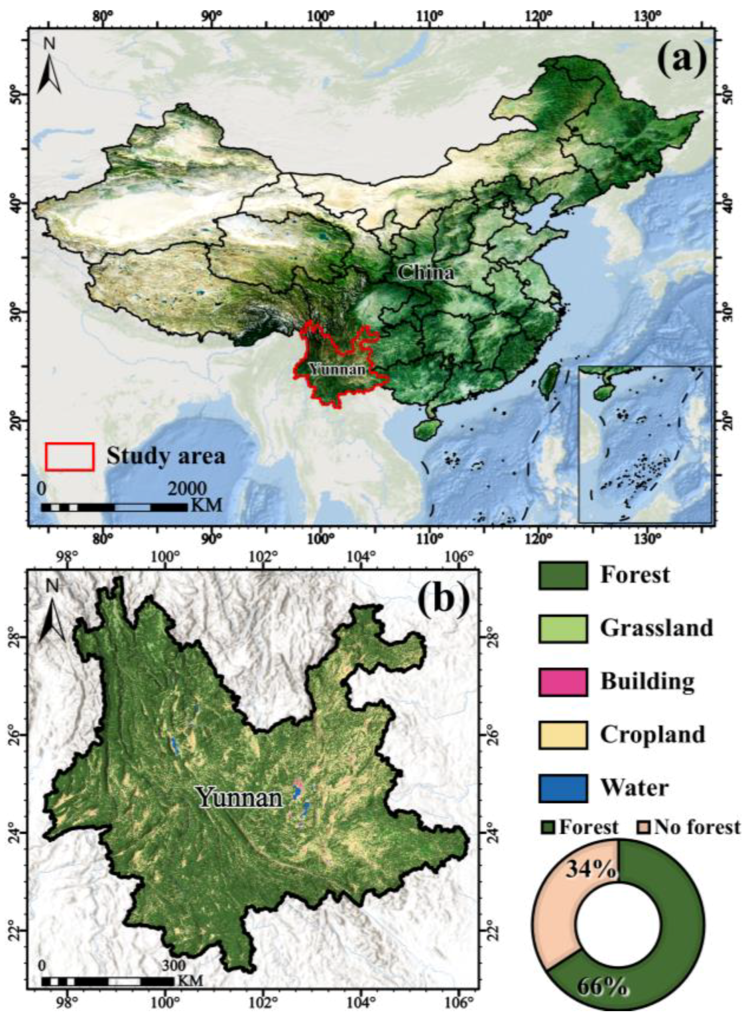
2.1. Study Area

Yunnan Province, located in southwestern China (Figure 1a), spans over 390,000 km2 and features a rugged, mountainous plateau terrain with elevations ranging from 79 m to 6740 m. The region experiences a subtropical monsoon climate, characterized by high temperatures and heavy rainfall throughout the year, with significant vertical temperature variation driven by topographic diversity. According to the State Forestry Administration of China (http://www.forestry.gov.cn, accessed on 1 May 2023), the forest cover in Yunnan exceeds 66% (Figure 1b), while vegetation cover surpasses 88%. The province is largely characterized by the low retention of primary natural forests, with approximately 70% comprising young, pure stands resulting from extensive afforestation efforts. In contrast, the primary forests in the southwestern region exhibit more complex species compositions due to their remote locations and low human population density along the border. The forests in the study area display exceptional species diversity, with dominant species such as Oak, Fir, Camphor, Eucalyptus, Masson Pine, Poplar, Cypress, and Simao Pine accounting for 70% of the total forest area. The region’s varied tree ages, species, landscapes, and levels of exploitation have resulted in diverse forest conditions and a highly complex understory community structure.

2.2. Data

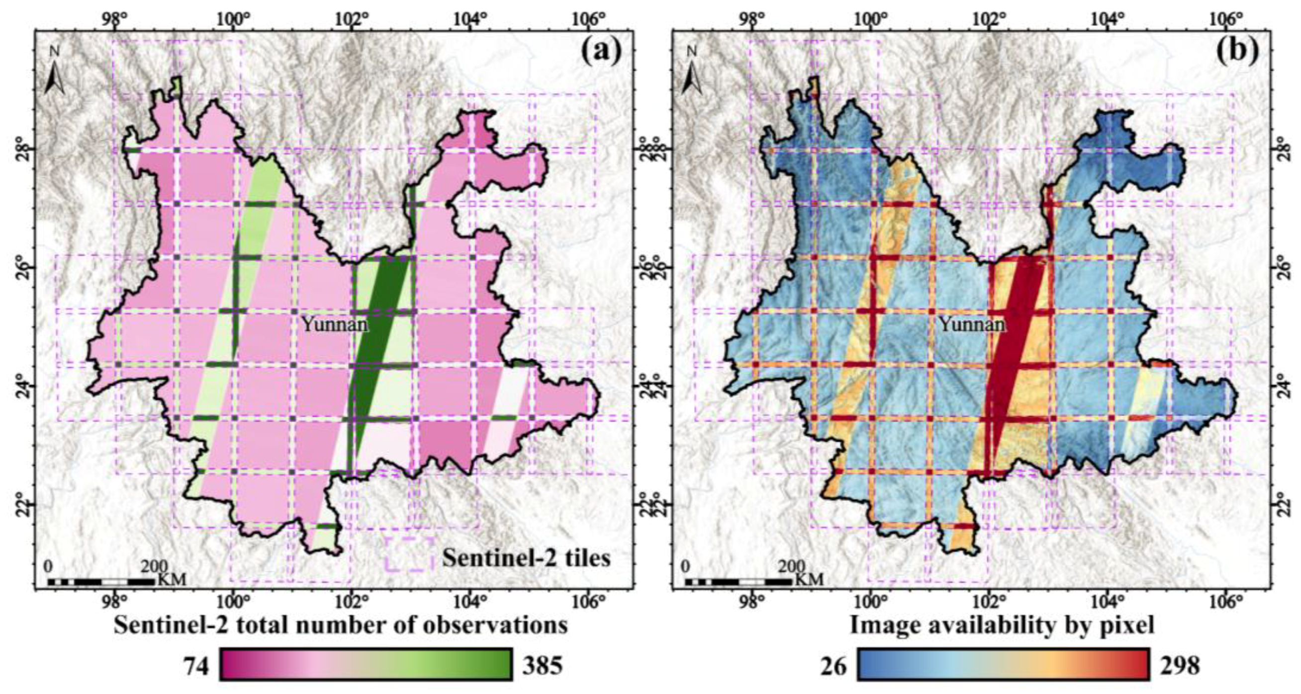
2.2.1. Sentinel-2 Time-Series Data

The large size of the study area and frequent cloud cover make it difficult to obtain cloud-free, fully covered Sentinel-2 data. To ensure sufficient image data for time-series modeling, all Sentinel-2 surface reflectance images from 2022 to 2023 with less than 20% cloud cover were retrieved (Figure 2). A de-cloud mask was then applied to each image using the quality assessment band “QA60”. To minimize the impact of cloud cover, shadows, and orbital variations, a median synthesis method was used to combine the raw images. Given the variable meteorological conditions, the synthesis time step was adjusted in 5-day increments, depending on the proportion of null regions in the synthesized images, until the proportion of null regions was less than 15%. This process resulted in 13 high-quality Sentinel-2 images that met the requirements. The following bands were retained for each image: visible (B2–B4), red-edge (B5–B7), near-infrared (B8), and short-wave infrared (B11–B12). The nearest neighbor method was used to resample all the spectral bands from 20 m to 10 m resolution, ensuring pixel matching with the 10 m resolution spectral bands.
The authors of this study then calculated various vegetation indices to assess the spectral separability of dominant tree species in the area using the JM distance for different indices and their combinations. The best-performing indices—Normalized Difference Vegetation Index (NDVI), Soil Adjustment Vegetation Index (SAVI), Ratio Vegetation Index (RVI), Near-Infrared Reflection of Vegetation (NIRV), Red Edge Inflection Point Index (REIP), and Enhanced Vegetation Index (EVI)—were finally selected. Detailed information and calculation formulas for each vegetation index are provided in Table 1.
Most images contain randomly distributed null regions due to the de-clouding process, which indicates missing spectral bands and vegetation indices. To avoid sample loss and anomalies in the time series caused by these missing values, all images were stacked as a whole and then interpolated using a cubic spline function to fill the null values. The continuous time series images were then smoothed using the S-G filter to reduce noise and remove outliers. Data acquisition and index calculations were performed using the Google Earth Engine (GEE) platform, while the time-series interpolation was carried out using Python 3.7.0.

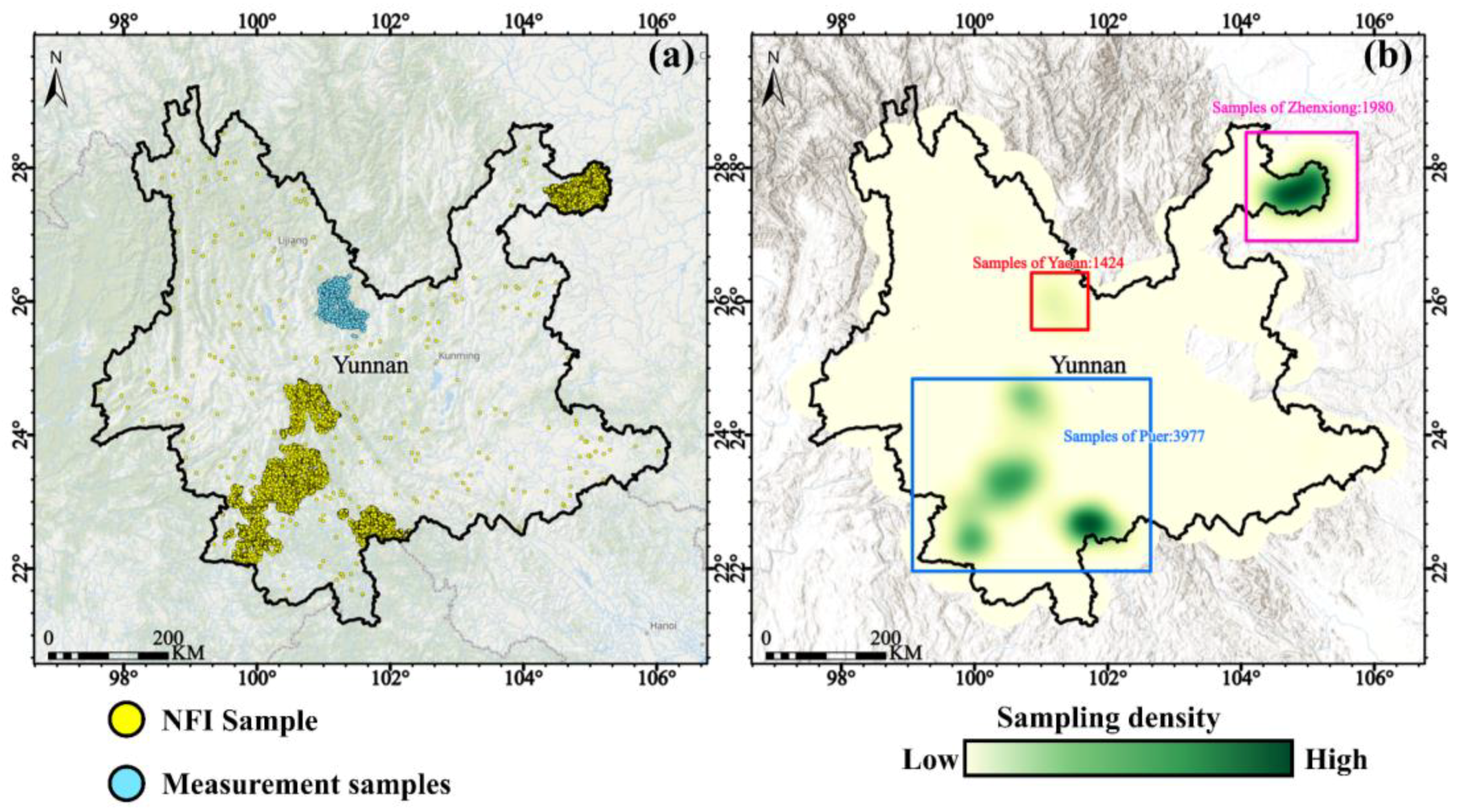
2.2.2. Tree Species Reference Data

The tree reference data for this study were sourced from the National Forest Inventory (NFI) data and field measurements. The NFI dataset, compiled by the China Forestry Bureau in 2022, provides a detailed description of forest information in Yunnan Province. The dataset includes forest plots as vector elements. Among them, the NFI data acquired in this study cover a seamless outline of Puer City and Zhenxiong County (Figure 3). The attribute fields include tree type, health status, origin, and the diameter at breast height (DBH). Quality checking of the NFI data was performed using the field filtering tool in ArcGIS Pro 3.0. Forest plots with the following characteristics were retained: (1) canopy cover > 0.2 (plots with less than 0.2 are considered non-forested by the Chinese Forestry Administration); (2) area > 1200 m2 to exclude fragmented patches, ensuring that the spectral information corresponding to the patches is representative; (3) pure forest type; and (4) excellent health status. The filtered forest patches were overlaid with 10 m resolution land cover data from Esri (2022) [35], and any patches containing non-forest pixels were removed. The retained NFI data were then imported into Google Earth for further visual inspection. Polygons with (1) incorrect boundaries, (2) disturbances (e.g., logging, pests, and diseases) from 2022 to 2023, or (3) non-forest features (e.g., bare ground) were excluded. This process resulted in 6321 regionally representative NFI forest patches. Field data were collected from June 2022 to May 2023 in the Yaoan area through field surveys. The selection criteria for field plots were consistent with those used for the NFI data. In addition, tree height and DBH within the plots were measured using a tape measure and laser altimeter. Plots with an average tree height of <5 m and an average DBH of <2 cm were excluded. Latitude and longitude for each plot’s center were recorded using the “Ovital 10.3.8” measurement software (https://www.ovital.com, accessed on 1 January 2025). Subsequently, the canopy cover for each plot was recorded using Digital Image Field Survey 3.2.5 software. Tree-type information was recorded only after consensus among multiple forestry experts. A total of 1424 tree species measurements were recorded for this study. Finally, each vector surface element in the NFI data was converted to points and merged with the latitude and longitude of the corresponding measured plots. A consistent coordinate system was applied to all vector data. These steps resulted in a total of 7745 high-quality sample data points, including attributes such as species type and canopy cover. The number of samples for each tree species is shown in Table 2.

2.2.3. Auxiliary Data

Topographic data, including elevation, slope, and slope direction bands, were sourced from the 30 m resolution SRTM Digital Elevation Data Version 4, hosted on the GEE platform. Geographic location information is crucial for understanding tree species distribution patterns, reflecting their adaptation to varying climatic and soil conditions. In this study, the latitude and longitude coordinates for each Sentinel-2 image center were recorded as separate bands. These coordinates, along with the topographic data, were used as auxiliary data to aid in the construction of the classification model.

3. Methods

3.1. Constructing the Classification Model for Tree Species

Given the challenges of high dimensionality and nonlinearity in time-series remote sensing data for forest mapping, this study employs the random forest algorithm, known for its robust performance in handling complex datasets with multiple covariances. This algorithm is well regarded in forest mapping tasks [36]. This study utilizes time series remote sensing data (primary bands and vegetation indices), environmental auxiliary data (elevation, slope and aspect variables), and multi-source tree species reference data to construct a random forest classification model. A random number band was introduced for tree species samples, generating floating numbers between 0 and 1, to prevent the same sample from being used for both training and validation in the model. The samples were then split into training and validation sets at a 7:3 ratio. The key parameters influencing the classification performance of the random forest model are the number of decision trees (n_tree) and the maximum tree depth (max_depth). To optimize model accuracy, 20% of the samples were randomly chosen for hyperparameter tuning. The model’s hyperparameters were set with n_tree ranging from 0 to 500 and max_depth from 0 to 30. A grid search method identified the optimal hyperparameter combinations for subsequent model training using the full sample dataset. Model accuracy was validated by (1) evaluating the overall accuracy (OA), Kappa coefficient (Ka), producer accuracy (PA), and user accuracy (UA) using the confusion matrix as well as (2) comparing the fitted NFI data of Puer City and Zhenxiong County with the distribution of dominant species in the predicted tree species map.

3.2. Calculation of Classification Uncertainty

Each decision tree in the random forest algorithm processes a subsample that includes location information, tree species categories, and predictor variables. During the prediction phase, each decision tree votes on the category of an unknown pixel based on its trained data. The combined votes from all trees determine the category probability for that pixel. The pixel’s final classification is assigned based on the maximum category probability, which reflects the model’s confidence in its classification. A higher maximum category probability indicates minimal interference from other categories, suggesting stronger spectral separability for that pixel. Conversely, a lower maximum category probability suggests that the model faces significant uncertainty in classifying the pixel, as it must choose a category with only a slight advantage over others due to the influence of competing category probabilities. In this study, the maximum category probability for each pixel is mosaiced as a separate band. Categorization uncertainty is calculated by subtracting the maximum category probability from 1.

3.3. Modeling Canopy Cover Inversion

Canopy cover measures the extent of understory exposure—such as bare soil and herbaceous plants—within an image element, defined as the proportion of an area shaded by the forest canopy per unit area when projected vertically. Similarly, canopy cover also indicates the extent of mixing between forest spectral information and understory background spectral data within a pixel. Higher canopy coverage results in a greater proportion of forest spectral information in the image, while lower coverage increases spectral confusion from the understory. To estimate forest canopy cover in the study area, this study employed the random forest algorithm, utilizing 7745 samples with canopy cover data and time-series remote sensing data (primary bands and vegetation indices) to develop a canopy cover inversion model. The inversion model used a range of hyperparameters consistent with the classification algorithm, which were optimized using the grid search method. The final inversion model was tuned with the optimal combination of hyperparameters, and the accuracy of the canopy cover estimates was assessed using the R2 and RMSE metrics.

3.4. Assessing the Relationship Between Canopy Cover and Classification Uncertainty

This study generated raster data for both classification uncertainty and canopy cover based on the described methodology. This study used two approaches to quantify the relationship between classification uncertainty and canopy cover: (1) To illustrate the spatial relationship between classification uncertainty and canopy cover, canopy cover was categorized according to the Chinese government’s criteria system (available at https://www.gov.cn, accessed on 1 May 2023). This system grades canopy cover in steps of 0.2 as follows: low cover (0.2–0.4), medium coverage (0.4–0.6), and high coverage (>0.6). Classification uncertainty was graded using the natural breakpoint method. These graded variables were then aggregated into 20 km × 20 km grid cells based on the majority of values within each cell. The relationships between the grades within these grids were visualized using binary contour plots. The grid size was determined through several manual tests to optimize visualization and analysis. (2) To further quantify the correlation between classification uncertainty and canopy cover, 2000 pixels were randomly sampled across different canopy cover classes. Each class served as a mask to isolate specific data for analysis. The correlation between classification uncertainty and canopy cover within these classes was then evaluated using Pearson’s correlation coefficient.

4. Results

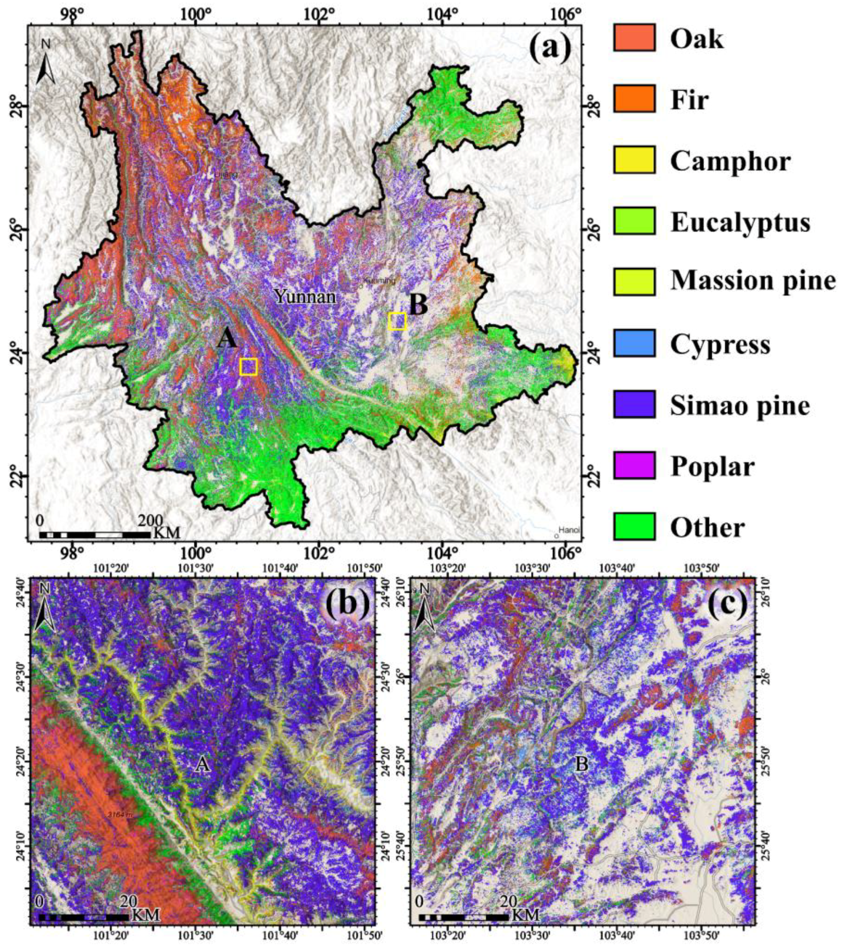
4.1. Projected Map of Dominant Tree Species

In this study, dominant tree species in Yunnan Province, China, were mapped with a 10 m spatial resolution, accurately classifying over 70% of the forest image elements. In addition, our map shows the spatial distribution of nine dominant tree species, highlighting the diversity of forest ecosystems in Yunnan (Figure 4). The distribution of dominant tree species across Yunnan Province varies significantly with elevation, showing distinct patterns as elevation decreases from the western highlands to the east lowlands. Oak and Fir are prevalent in the high-altitude regions of the western and northwestern parts of the province, whereas the primary forests in the southwestern parts are sparsely populated, less exploited, and host rare species. In central Yunnan’s lower elevations, Cypress, Simao Pine, and Eucalyptus are predominantly found. Additionally, Oak and Fir continue to densely populate some of the high-altitude mountainous areas within the region. Further decrease in altitude sees an abundance of Eucalyptus in the northeast, with Poplar being more prevalent in the east. Cypress and Masson Pine line the roads in the more developed areas of the southeast, reflecting their value in wood processing. These species are extensively planted in accessible areas to facilitate easy transport and processing for wood production.

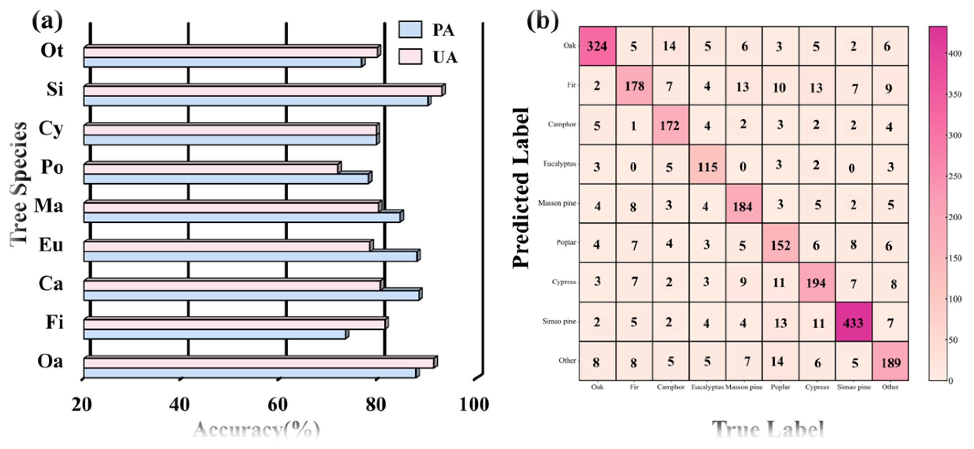
4.2. Classification Model Mapping Accuracy

The classification model achieved an overall accuracy of 83.52% and a Kappa coefficient of 0.8115 with the optimal hyperparameter combinations for tree species mapping. This high accuracy indicates the strong model performance of the classification model in identifying dominant tree species in Yunnan Province. The Kappa coefficient further supports the model’s reliability, indicating a well-balanced classification across tree species and confirming the objectivity and relevance of the results. To assess the model’s performance in greater detail, we analyzed the confusion matrix along with producer and user accuracy metrics (Figure 5). Nearly all tree species achieved a producer and user accuracy exceeding 80%, with species such as Oak and Simao Pine achieving accuracies above 90% (Figure 5a). In contrast, Fir and Poplar showed the lowest accuracy values, suggesting that these species are more prone to misclassification due to their spectral similarities with other species. Further examination of the confusion matrix (Figure 5b) revealed some interspecific confusion. Oak was frequently misclassified as Camphor, and Fir was often mistaken for Masson Pine and Cypress, likely due to similarities in canopy structure, leaf morphology, and phenological traits. Eucalyptus and Camphor, both broadleaf species, were often confused with each other. Masson Pine was commonly misidentified as Fir, while Poplar exhibited high confusion with nearly all other species, possibly due to sample quality issues. Lastly, Cypress was often misclassified as Fir, Masson Pine, or Poplar, and Masson Pine was also frequently identified as Poplar and Cypress.
Figure 6 illustrates the significant linear relationship between the predicted tree species map and the area proportions of each tree species in the seamless NFI data for Zhenxiong County and Puer City. For both regions, the R2 values greater than 0.93, and the RMSE values were below 2.6. In Zhenxiong County, the predicted species map showed an R2 of 0.933 and an RMSE of 1.292. In Puer City, the R2 was 0.959 with an RMSE of 2.52. These results demonstrate a high degree of agreement between the predicted tree species distribution and the actual area proportions, further confirming the accuracy and credibility of the tree map.

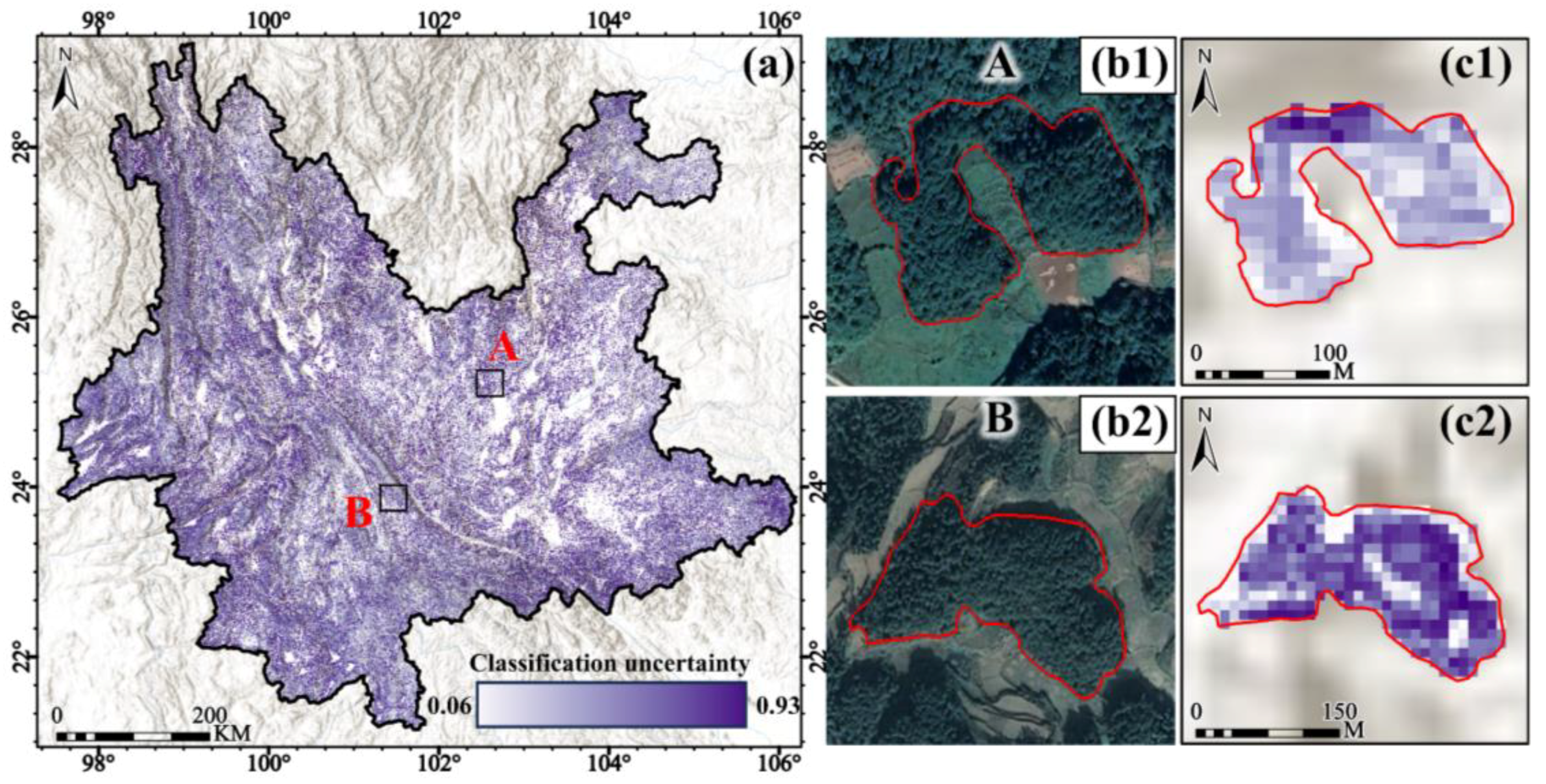
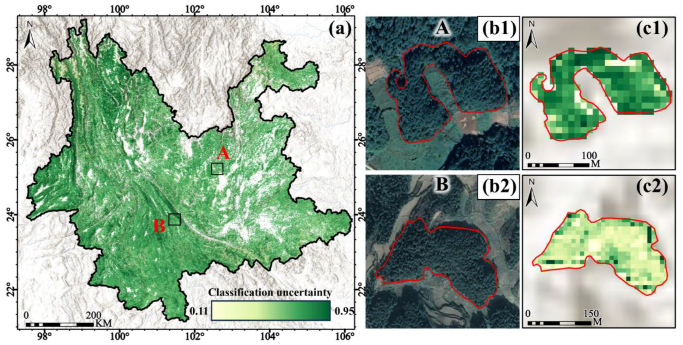
4.3. Results of Classification Uncertainty

The categorical uncertainty reported by the classification model was extracted as a separate band to illustrate its spatial distribution prior to category label assignment. The uncertainty values ranged from 0.06 to 0.93 (Figure 7), with higher uncertainty observed in the western and southern parts of the study area and lower uncertainty in the central and eastern regions. As shown in Figure 4, tree species such as Oak, Fir, and Simao Pine, found in the central mountainous areas, exhibit lower categorical uncertainty, while Masson Pine, located in the south and northeast, shows higher classification uncertainty. Additionally, the “other” category, representing mixed species in the southwest, exhibited stronger taxonomic uncertainty. At the local scale, taxonomic uncertainty did not appear to be related to the degree of tree cover within the plots, as seen in Figure 7(b1–c2). For example, two high-resolution satellite imagery plots, both densely planted with healthy trees and exhibiting uniform tree textures, demonstrated significant differences in classification uncertainty. Plot A, with a larger canopy and stronger canopy overlap effect, showed lower uncertainty, whereas Plot B, with smaller canopies and more exposed understory, displayed higher uncertainty.

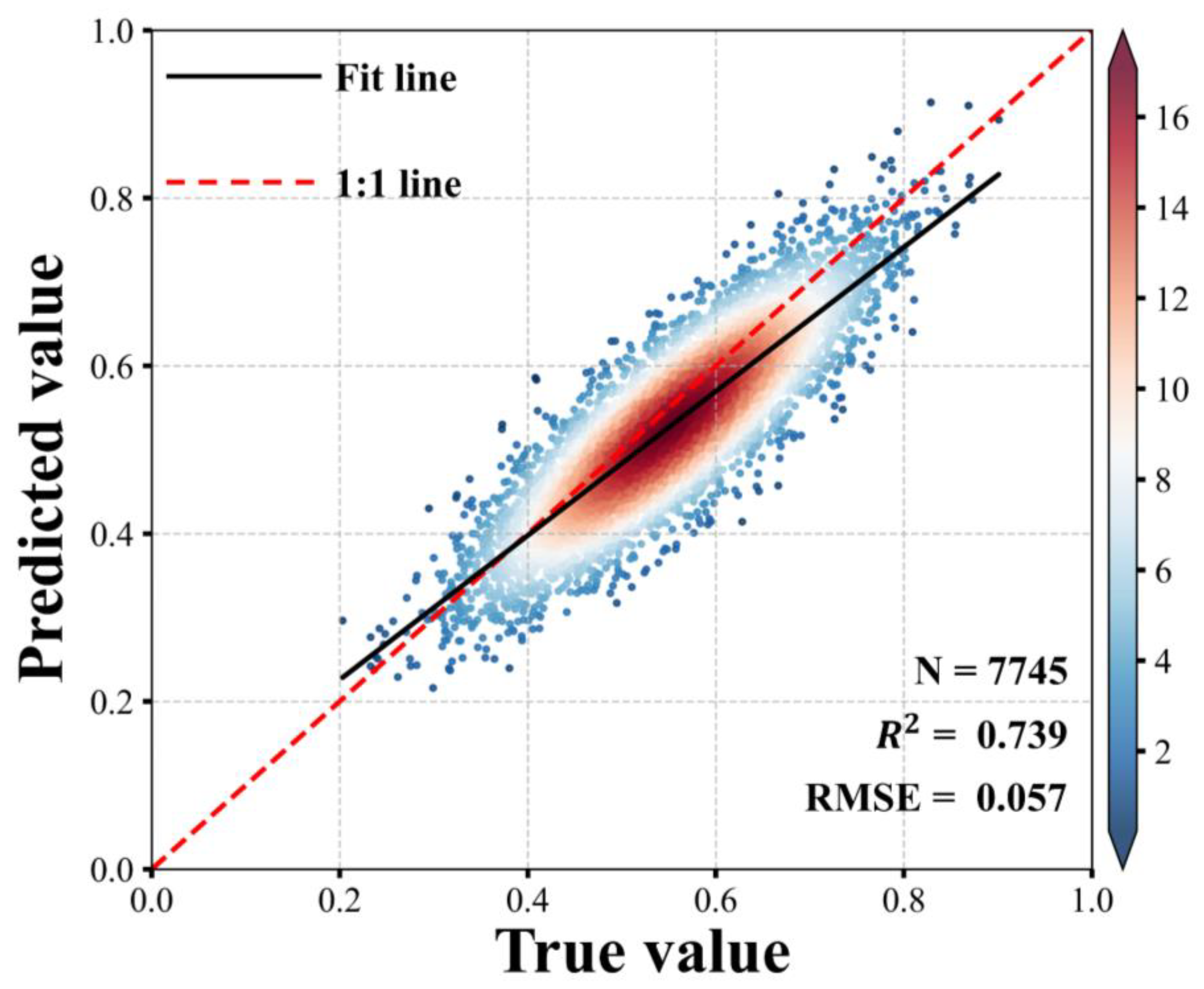
4.4. Canopy Cover Inversion Results and Inversion Accuracy

Figure 8 illustrates the inversion results of forest canopy cover in Yunnan Province, derived using the random forest inversion model. The canopy cover values in the study area show significant variation, ranging from 0.11 to 0.95. Primary forests in the northern and southern mountainous regions exhibit higher canopy cover, indicating a high degree of canopy overlap, which minimizes the influence of the understory background on the image elements. In contrast, forests in the southwestern and northeastern parts also show relatively high canopy cover, while the southern and east-central regions possess the lowest values. These regions likely have smaller crowns and lower canopy density due to species differences, age, and stand conditions, resulting in greater exposure of the understory, which may have produced a stronger mixing effect. At the local scale, the canopy cover distribution in example plots A and B revealed notable differences. Plot A, with a larger canopy and greater canopy overlap, demonstrated higher canopy cover, while plot B, with a smaller canopy, had lower canopy cover values across all image elements. The R2 of the canopy cover inversion in this study was 0.739, with an RMSE of 0.057 (Figure 9), confirming the predictive accuracy and reliability of the inversion model.

4.5. Relationship Between Canopy Cover and Classification Uncertainty

The binary contour plot in Figure 10 confirms our hypothesis that greater canopy cover is associated with lower classification uncertainty. Conversely, areas with lower canopy cover tend to exhibit higher classification uncertainty. As shown in Figure 10c, the southeastern and east-central parts of the study area are characterized by low canopy cover and high classification uncertainty. In contrast, the southern and northwestern areas show high canopy cover and low classification uncertainty. These patterns are particularly prevalent within the study area. According to Figure 10d, 76.67% of grids with low-canopy-cover areas exhibit moderate to high classification uncertainty. Of these, 35.42% showed high classification uncertainty, while only 23.33% exhibited low uncertainty. In areas of medium canopy cover, 86.64% of the grids showed medium and low classification uncertainty. The proportions of medium and low uncertainty are similar, while high uncertainty accounted for only 13.36%. Notably, in high-canopy-cover areas, 96.25% of the grids had low to medium classification uncertainty, with 75.12% exhibiting low uncertainty. High classification uncertainty decreased progressively with increasing canopy cover. In low-canopy-cover areas, high classification uncertainty was present in 35.42% of grids. This percentage dropped to 13.36% in areas with medium canopy cover. In high-canopy-cover areas, the percentage further decreased to only 3.75%. As the area of low classification uncertainty increased, the percentage of low uncertainty rose from 23.33% to 46.12%, ultimately reaching 75.12%. These findings suggest a clear negative relationship between canopy cover and classification uncertainty, particularly in high-canopy-cover areas.
Figure 11 illustrates the correlation between canopy cover and classification uncertainty at the pixel level across different canopy cover regions. Randomly sampled validation points within each region show a negative correlation between canopy cover and classification uncertainty. In the low-canopy-cover region, the correlation of the validation points is −0.67. In areas with medium canopy cover, the correlation is weaker at −0.40. Notably, in the high-canopy-cover region, the correlation reaches −0.73, indicating a strong negative relationship. This suggests that forests in areas with high canopy cover tend to have higher classification accuracy and lower classification uncertainty. The overall correlation between canopy cover and classification uncertainty is −0.54. This indicates that as canopy cover increases, the proportion of forest cover in the image increases, reducing the spectral confounding effect from the understory background. As a result, the classification model shows lower uncertainty and fewer potential errors in assigning category labels.

5. Discussion

This study used the random forest algorithm to map the dominant tree species in Yunnan Province at a 10 m resolution. Category attribution was accurately performed for 70% of the forest pixels, yielding an overall accuracy of 83.52%. To validate the model’s relationship between classification uncertainty and canopy cover, this study estimated the canopy cover of forests in the area, achieving an R2 value of 0.739. The relationship between classification uncertainty and canopy cover was quantified using binary contour maps at the grid scale and Pearson’s correlation at the pixel scale.

5.1. Limitations of Reference Data

The tree species reference data for this study were derived from a synthesis of forest inventory and field measurement data, subjected to strict quality control procedures. Eight dominant tree species, covering over 70% of the forested area in Yunnan Province, were selected for mapping, while other species were grouped into a single “Other” category. Although these eight species are the core components of the region’s forest ecosystems, the diversity within the “Other” category leads to misclassification during hard categorization. For instance, Nanya Pine, classified under the “Other” category, exhibits morphological, phenological, and spectral similarities with Masson Pine and Simao Pine, creating challenges in distinguishing it from the dominant species. This spectral similarity complicates accurate classification [22,27]. When uncommon species are classified separately, their small sample sizes result in low classification accuracy, ultimately affecting the overall accuracy of the model [37]. As Hemmerling et al. [10] found, these uncommon species are difficult to properly categorize due to their complex types and spectral similarities. Their limited samples make it still impossible to achieve sufficient accuracy in the classification process, and improving the accuracy of uncommon species often comes at the expense of overall accuracy, suggesting that there is a trade-off between detail and accuracy in cartography. Another significant concern is the reliability of the National Forest Inventory (NFI) data. While the NFI is the most comprehensive source of forest attribute data, the lengthy data collection and compilation processes by government agencies may introduce classification inconsistencies in plot-level data, often unrecorded. The professionalism and expertise of personnel involved in data compilation also contribute to potential errors. In this study, the NFI data exhibited numerous overlapping boundaries and incorrect plot locations, further limiting its reliability. These inherent limitations may constrain the accuracy of species mapping, highlighting the need to explore potential solutions to mitigate these issues.

5.2. Uncertainty Due to Background Spectral Mixing Effects in the Forest Understory

The combination of tree species, planting conditions, and other factors contributes to information impurity within forest pixels, which currently limits the accuracy of forest monitoring tasks. As noted by Li et al. [38], large gaps in sparse vegetation canopies allow the soil background to interfere with the forest signal, affecting the spectral reflectance of the forest. Similarly, Wan et al. [19] demonstrated that the mixing effect of the understory background—caused by canopy structure, leaf morphology, and soil—contaminates the forest spectrum, reducing the accuracy of leaf area index (LAI) inversion. However, most studies acknowledge this impact without quantifying its uncertainty in forest monitoring. This study addressed this gap by quantifying the relationship between canopy cover and classification uncertainty using binary contour plots and Pearson’s correlation coefficients at the grid and pixel scales. The results revealed that higher canopy cover is associated with lower classification uncertainty. This finding confirms that the spectral mixing effect, resulting from the interaction between the understory background and forest canopy, is strongly correlated with classification uncertainty. Nevertheless, the pervasive influence of the understory remains a challenge. Since canopy cover is considered a direct indicator of understory exposure, the correlation between canopy cover and classification uncertainty may appear ambiguous due to understory interference during inversion. To address this issue, existing studies propose the following solutions: (1) Construct a spectral library of understory backgrounds. For example, Weiss et al. [39] modeled the mixing pattern of soil and vegetation pixels through simulation to correct for the mixing effect before conducting forest monitoring. However, these methods often rely on a limited set of predefined spectral modes, making it challenging to capture diverse canopy structures and variations in site conditions. (2) Ensure a high percentage of forest canopy. This approach focuses on the use of high-spatial-resolution remotely sensed imagery to ensure a high proportion of the forest canopy in the image element. However, variations in canopy structure due to age, climatic stages, and planting patterns make it difficult to match the resolution accurately. Moreover, the high cost of acquiring high-resolution imagery limits the practical application of this method. The above problems make the spectral mixing effect from the forest background always constrain the confidence of the results. It lacks the effective means to correct mixed forest pixels. In addition, interspecies spectral mixing from mixed stands and intraspecies spectral variability from uneven-aged stands introduced additional mixing factors to the forest image element, resulting in unanticipated errors in assessing the relationship between understory background exposure and taxonomic uncertainty by relying on canopy cover alone. This is the direction of our future improvement.

6. Conclusions

In this study, we successfully mapped the dominant tree species in Yunnan Province at a 10 m resolution using time-series Sentinel-2 data and a random forest classification algorithm. To evaluate the influence of the understory background on classification accuracy, we employed a random forest inversion model to estimate forest canopy cover. The relationship between classification uncertainty and canopy cover was analyzed through binary contour plots at the grid scale and Pearson’s correlation coefficient at the pixel scale. The key conclusions drawn from the study are as follows:
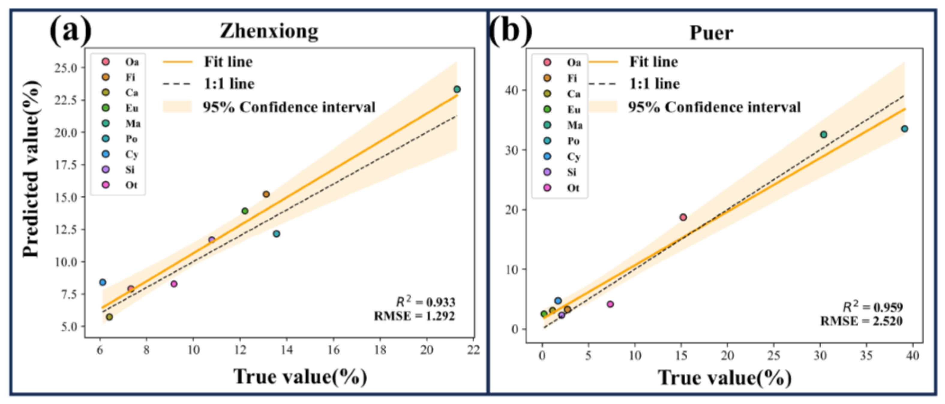
  • Applicability of time-series Sentinel-2 for tree species mapping: The integration of time-series Sentinel-2 data, vegetation index characteristics, and environmental variables enabled the accurate mapping of eight dominant tree species in Yunnan Province. The mapping achieved an overall accuracy of 83.52%, with a Kappa coefficient of 0.8115. The predicted tree species maps exhibited a strong agreement with National Forest Inventory (NFI) data, achieving an R2 value exceeding 0.93 and root mean square errors (RMSEs) below 2.6. These results validate the classification performance of the proposed framework and the reliability of the generated tree species maps.
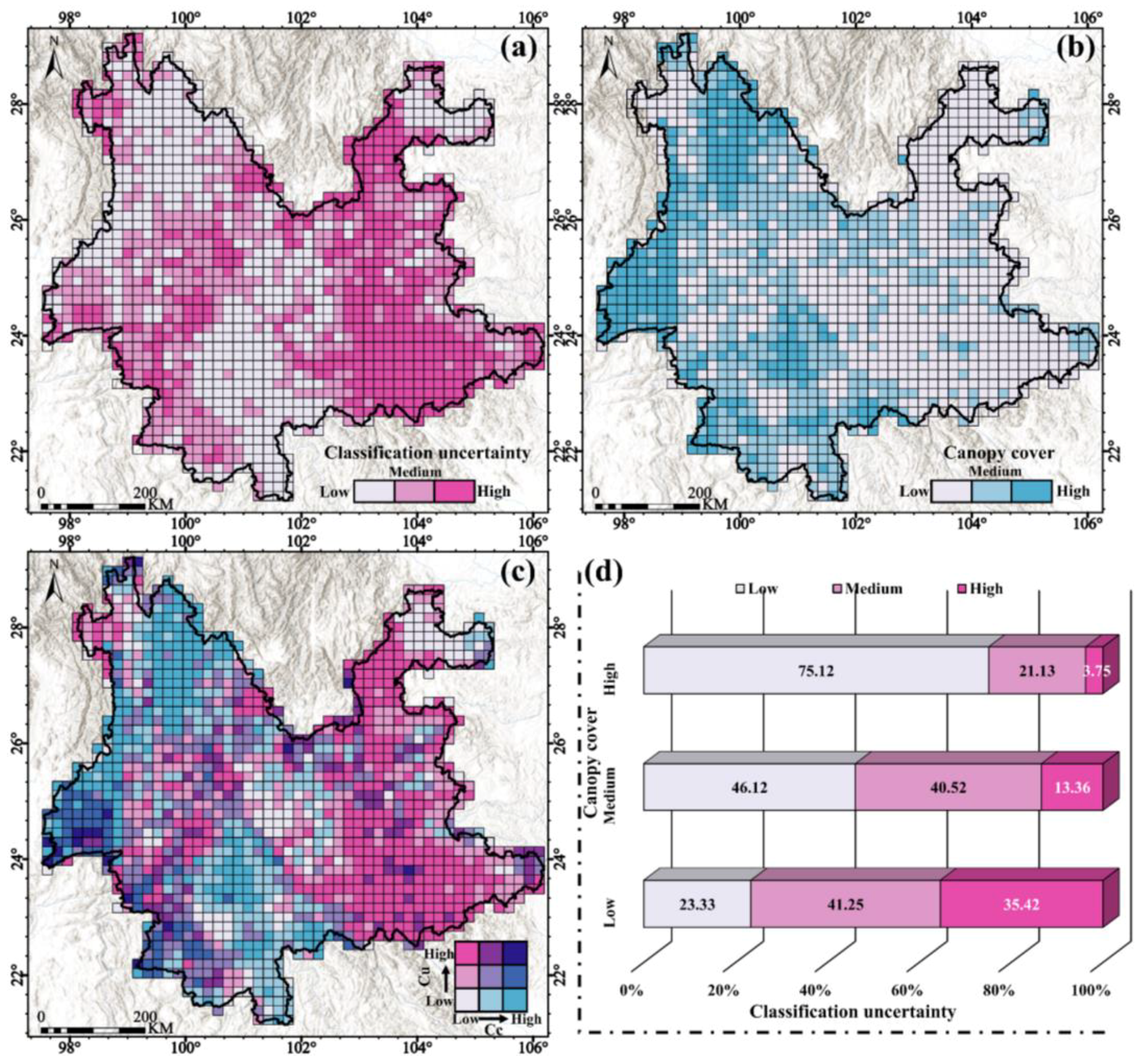
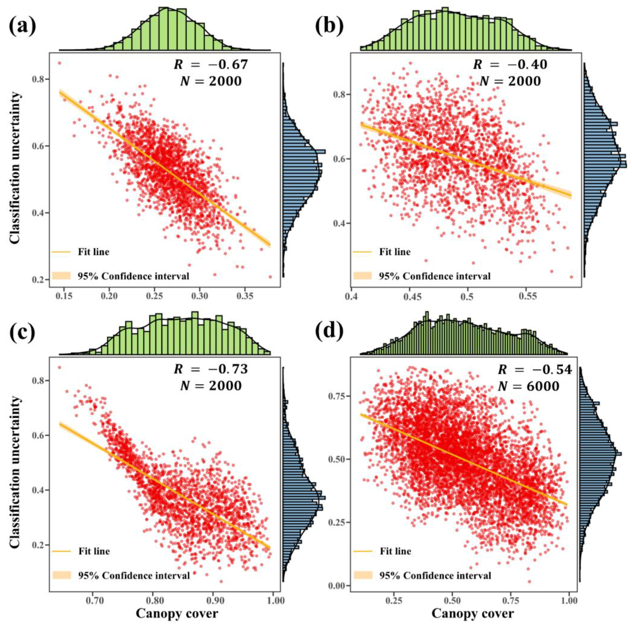
  • Understory background and classification uncertainty: Binary contour plots revealed that areas with high classification uncertainty decreased as canopy cover increased, while areas with low classification uncertainty expanded with lower canopy cover. The model demonstrated superior classification performance and greater confidence in regions with dense canopy cover. Pearson’s correlation analysis further confirmed a significant negative correlation between canopy cover and classification uncertainty, with an overall correlation coefficient of −0.54. In areas with low canopy cover, the correlation was 0.67. The correlation was −0.40 in the region of medium canopy cover. The correlation was −0.73 in the region of high canopy cover.

Author Contributions

Conceptualization, Y.S. and H.L.; methodology, Y.S.; software, Y.S.; validation, J.Z. and B.Y.; formal analysis, Y.S.; investigation, Y.S.; resources, B.Y.; data curation, J.Z. and B.Y.; writing—original draft preparation, Y.S.; writing—review and editing, B.Y.; visualization, Y.S.; supervision, H.L.; project administration, H.L.; funding acquisition, H.L. All authors have read and agreed to the published version of the manuscript.

Funding

This research was funded by the Young Scientists Fund of the National Natural Science Foundation of China (No. 32201557).

Data Availability Statement

The data are not publicly available due to privacy restrictions.

Acknowledgments

I would like to express my sincere gratitude to Beijing Yuansheng Huawei Software Co. and Wuxi Wei Le Cai Zhi Software Development Co., Ltd., for developing the “Ovital” and “Digital Image Field Survey” software, which significantly contributed to the success of this research. We thank the reviewers for their thoughtful comments and constructive suggestions, which substantially improved this manuscript.

Conflicts of Interest

The authors declare no conflicts of interest.

References

  1. Schelhaas, M.; Teeuwen, S.; Oldenburger, J.; Beerkens, G.; Velema, G.; Kremers, J.; Lerink, B.; Paulo, M.; Schoonderwoerd, H.; Daamen, W. Zevende Nederlandse Bosinventarisatie: Methoden en Resultaten; Wettelijke Onderzoekstaken Natuur & Milieu: Wageningen, The Netherlands, 2022; pp. 2352–2739. [Google Scholar]
  2. Wang, R.; Gamon, J.A. Remote sensing of terrestrial plant biodiversity. Remote Sens. Environ. 2019, 231, 111218. [Google Scholar] [CrossRef]
  3. Xiao, J.; Chevallier, F.; Gomez, C.; Guanter, L.; Hicke, J.A.; Huete, A.R.; Ichii, K.; Ni, W.; Pang, Y.; Rahman, A.F. Remote sensing of the terrestrial carbon cycle: A review of advances over 50 years. Remote Sens. Environ. 2019, 233, 111383. [Google Scholar] [CrossRef]
  4. Young, B.; Yarie, J.; Verbyla, D.; Huettmann, F.; Herrick, K.; Chapin, F.S. Modeling and mapping forest diversity in the boreal forest of interior Alaska. Landsc. Ecol. 2017, 32, 397–413. [Google Scholar] [CrossRef]
  5. Gillis, M.D.; Leckie, D.G. Forest Inventory Mapping Procedures Across Canada; Information Report No. PI-X-114; Petawawa National Forestry Institute: Chalk River, ON, Canada, 1993. [Google Scholar]
  6. Tomppo, E.; Gschwantner, T.; Lawrence, M.; McRoberts, R.E.; Gabler, K.; Schadauer, K.; Vidal, C.; Lanz, A.; Ståhl, G.; Cienciala, E. Pathways for Common Reporting. In National Forest Inventories; European Science Foundation: Strasbourg, France, 2010; Volume 1, pp. 541–553. [Google Scholar]
  7. White, J.C.; Coops, N.C.; Wulder, M.A.; Vastaranta, M.; Hilker, T.; Tompalski, P. Remote sensing technologies for enhancing forest inventories: A review. Can. J. Remote Sens. 2016, 42, 619–641. [Google Scholar] [CrossRef]
  8. Matasci, G.; Hermosilla, T.; Wulder, M.A.; White, J.C.; Coops, N.C.; Hobart, G.W.; Bolton, D.K.; Tompalski, P.; Bater, C.W. Three decades of forest structural dynamics over Canada’s forested ecosystems using Landsat time-series and lidar plots. Remote Sens. Environ. 2018, 216, 697–714. [Google Scholar] [CrossRef]
  9. Ørka, H.O.; Jutras-Perreault, M.-C.; Næsset, E.; Gobakken, T. A framework for a forest ecological base map–An example from Norway. Ecol. Indic. 2022, 136, 108636. [Google Scholar] [CrossRef]
  10. Hemmerling, J.; Pflugmacher, D.; Hostert, P. Mapping temperate forest tree species using dense Sentinel-2 time series. Remote Sens. Environ. 2021, 267, 112743. [Google Scholar] [CrossRef]
  11. Francini, S.; Schelhaas, M.-J.; Vangi, E.; Lerink, B.; Nabuurs, G.-J.; McRoberts, R.E.; Chirici, G. Forest species mapping and area proportion estimation combining Sentinel-2 harmonic predictors and national forest inventory data. Int. J. Appl. Earth Obs. Geoinf. 2024, 131, 103935. [Google Scholar] [CrossRef]
  12. Nasiri, V.; Beloiu, M.; Asghar Darvishsefat, A.; Griess, V.C.; Maftei, C.; Waser, L.T. Mapping tree species composition in a Caspian temperate mixed forest based on spectral-temporal metrics and machine learning. Int. J. Appl. Earth Obs. Geoinf. 2023, 116, 103154. [Google Scholar] [CrossRef]
  13. Waser, L.T.; Küchler, M.; Jütte, K.; Stampfer, T. Evaluating the Potential of WorldView-2 Data to Classify Tree Species and Different Levels of Ash Mortality. Remote Sens. 2014, 6, 4515–4545. [Google Scholar] [CrossRef]
  14. Fassnacht, F.E.; Latifi, H.; Stereńczak, K.; Modzelewska, A.; Lefsky, M.; Waser, L.T.; Straub, C.; Ghosh, A. Review of studies on tree species classification from remotely sensed data. Remote Sens. Environ. 2016, 186, 64–87. [Google Scholar] [CrossRef]
  15. Shang, C.; Coops, N.C.; Wulder, M.A.; White, J.C.; Hermosilla, T. Update and spatial extension of strategic forest inventories using time series remote sensing and modeling. Int. J. Appl. Earth Obs. Geoinf. 2020, 84, 101956. [Google Scholar] [CrossRef]
  16. Hermosilla, T.; Bastyr, A.; Coops, N.C.; White, J.C.; Wulder, M.A. Mapping the presence and distribution of tree species in Canada’s forested ecosystems. Remote Sens. Environ. 2022, 282, 113276. [Google Scholar] [CrossRef]
  17. Hościło, A.; Lewandowska, A. Mapping forest type and tree species on a regional scale using multi-temporal Sentinel-2 data. Remote Sens. 2019, 11, 929. [Google Scholar] [CrossRef]
  18. Pasquarella, V.J.; Holden, C.E.; Woodcock, C.E. Improved mapping of forest type using spectral-temporal Landsat features. Remote Sens. Environ. 2018, 210, 193–207. [Google Scholar] [CrossRef]
  19. Wan, L.; Ryu, Y.; Dechant, B.; Hwang, Y.; Feng, H.; Kang, Y.; Jeong, S.; Lee, J.; Choi, C.; Bae, J. Correcting confounding canopy structure, biochemistry and soil background effects improves leaf area index estimates across diverse ecosystems from Sentinel-2 imagery. Remote Sens. Environ. 2024, 309, 114224. [Google Scholar] [CrossRef]
  20. Mandl, L.; Viana-Soto, A.; Seidl, R.; Stritih, A.; Senf, C. Unmixing-based forest recovery indicators for predicting long-term recovery success. Remote Sens. Environ. 2024, 308, 114194. [Google Scholar] [CrossRef]
  21. Farwell, L.S.; Gudex-Cross, D.; Anise, I.E.; Bosch, M.J.; Olah, A.M.; Radeloff, V.C.; Razenkova, E.; Rogova, N.; Silveira, E.M.; Smith, M.M. Satellite image texture captures vegetation heterogeneity and explains patterns of bird richness. Remote Sens. Environ. 2021, 253, 112175. [Google Scholar] [CrossRef]
  22. Zeug, G.; Immitzer, M.; Neuwirth, M.; Atzberger, C. Machbarkeitsstudie zur Nutzung von Satellitenfernerkundungsdaten (Copernicus) für Zwecke der Ableitung Ökologischer Belastungsgrenzen und der Verifizierung von Indikatoren der Deutschen Anpassungsstrategie an den Klimawandel: Feasibility Study on the Use of Earth Observation Data for the Purpose of Determining Ecological Exposure Limits and for the Verification of Indicators of the German Adaptation Strategy to Climate Change; Terranea UG: Geltendorf, Germany, 2018. [Google Scholar]
  23. Sudmanns, M.; Tiede, D.; Augustin, H.; Lang, S. Assessing global Sentinel-2 coverage dynamics and data availability for operational Earth observation (EO) applications using the EO-Compass. Int. J. Digit. Earth 2020, 13, 768–784. [Google Scholar] [CrossRef] [PubMed]
  24. Kollert, A.; Bremer, M.; Löw, M.; Rutzinger, M. Exploring the potential of land surface phenology and seasonal cloud free composites of one year of Sentinel-2 imagery for tree species mapping in a mountainous region. Int. J. Appl. Earth Obs. Geoinf. 2021, 94, 102208. [Google Scholar] [CrossRef]
  25. Blickensdörfer, L.; Oehmichen, K.; Pflugmacher, D.; Kleinschmit, B.; Hostert, P. National tree species mapping using Sentinel-1/2 time series and German National Forest Inventory data. Remote Sens. Environ. 2024, 304, 114069. [Google Scholar] [CrossRef]
  26. Dong, T.; Liu, J.; Liu, J.; He, L.; Wang, R.; Qian, B.; McNairn, H.; Powers, J.; Shi, Y.; Chen, J.M. Assessing the consistency of crop leaf area index derived from seasonal Sentinel-2 and Landsat 8 imagery over Manitoba, Canada. Agric. For. Meteorol. 2023, 332, 109357. [Google Scholar] [CrossRef]
  27. Grabska, E.; Frantz, D.; Ostapowicz, K. Evaluation of machine learning algorithms for forest stand species mapping using Sentinel-2 imagery and environmental data in the Polish Carpathians. Remote Sens. Environ. 2020, 251, 112103. [Google Scholar] [CrossRef]
  28. Wang, J.; Lopez-Lozano, R.; Weiss, M.; Buis, S.; Li, W.; Liu, S.; Baret, F.; Zhang, J. Crop specific inversion of PROSAIL to retrieve green area index (GAI) from several decametric satellites using a Bayesian framework. Remote Sens. Environ. 2022, 278, 113085. [Google Scholar] [CrossRef]
  29. Broge, N.; Mortensen, J. Deriving green crop area index and canopy chlorophyll density of winter wheat from spectral reflectance data. Remote Sens. Environ. 2002, 81, 45–57. [Google Scholar] [CrossRef]
  30. Bolyn, C.; Michez, A.; Gaucher, P.; Lejeune, P.; Bonnet, S. Forest mapping and species composition using supervised per pixel classification of Sentinel-2 imagery. Biotechnol. Agron. Soc. Environ. 2018, 22, 16. [Google Scholar] [CrossRef]
  31. Jordan, C.F. Derivation of Leaf-Area Index from Quality of Light on the Forest Floor. Ecology 1969, 50, 663–666. [Google Scholar] [CrossRef]
  32. Badgley, G.; Field, C.B.; Berry, J.A. Canopy near-infrared reflectance and terrestrial photosynthesis. Sci. Adv. 2017, 3, e1602244. [Google Scholar] [CrossRef]
  33. Martimort, P.; Fernandez, V.; Kirschner, V.; Isola, C.; Meygret, A. Sentinel-2 MultiSpectral imager (MSI) and calibration/validation. In Proceedings of the 2012 IEEE International Geoscience and Remote Sensing Symposium, Munich, Germany, 22–27 July 2012; pp. 6999–7002. [Google Scholar]
  34. Huete, A.; Didan, K.; Miura, T.; Rodriguez, E.P.; Gao, X.; Ferreira, L.G. Overview of the radiometric and biophysical performance of the MODIS vegetation indices. Remote Sens. Environ. 2002, 83, 195–213. [Google Scholar] [CrossRef]
  35. Karra, K.; Kontgis, C.; Statman-Weil, Z.; Mazzariello, J.C.; Mathis, M.; Brumby, S.P. Global land use/land cover with Sentinel-2 and deep learning. In Proceedings of the IGARSS 2021–2021 IEEE International Geoscience and Remote Sensing Symposium. IEEE, Brussels, Belgium, 11–16 July 2021. [Google Scholar]
  36. Belgiu, M.; Drăguţ, L. Random forest in remote sensing: A review of applications and future directions. ISPRS J. Photogramm. Remote Sens. 2016, 114, 24–31. [Google Scholar] [CrossRef]
  37. Wulder, M.A.; Hermosilla, T.; White, J.C.; Coops, N.C. Biomass status and dynamics over Canada’s forests: Disentangling disturbed area from associated aboveground biomass consequences. Environ. Res. Lett. 2020, 15, 094093. [Google Scholar] [CrossRef]
  38. Li, L.; Mu, X.; Qi, J.; Pisek, J.; Roosjen, P.; Yan, G.; Huang, H.; Liu, S.; Baret, F. Characterizing reflectance anisotropy of background soil in open-canopy plantations using UAV-based multiangular images. ISPRS J. Photogramm. Remote Sens. 2021, 177, 263–278. [Google Scholar] [CrossRef]
  39. Weiss, M.; Baret, F.; Jay, S. S2ToolBox Level 2 products: LAI, FAPAR, FCOVER. Available online: https://step.esa.int/docs/extra/ATBD_S2ToolBox_L2B_V1.1.pdf (accessed on 1 January 2025).
Figure 1. Overview map of the study area. (a) indicates the location of the study area in China. (b) indicates the distribution of forests in the study area.
Forests 16 00272 g001
Figure 2. Sentinel-2 image usability within the study area. (a) shows the overall image usability. (b) shows the pixel-by-pixel image usability.
Forests 16 00272 g002
Figure 3. Map of sampling distribution in the study area. (a) represents the spatial distribution of samples from different sources in the study area. (b) represents the sampling density in the study area.
Forests 16 00272 g003
Figure 4. Predicted dominant tree species in the study area. (a) represents the spatial distribution of overall dominant tree species within the study area. (b) and (c) represent detailed tree species distribution information within individual areas (A and B).
Forests 16 00272 g004
Figure 5. Producer accuracy, user accuracy, and confusion matrix results for each tree species. (a) represents the producer accuracy, and user accuracy of each tree species reported by the classification model. The meanings of the abbreviations in the vertical axis are shown in Table 2. PA stands for producer accuracy and UA stands for user accuracy. (b) represents the confusion matrix.
Forests 16 00272 g005
Figure 6. Linear fit between NFI data and area share of dominant tree species in predicted tree map for Zhenxiong (a) and Puer (b). The meanings of the abbreviated letters in the figure are shown in Table 2.
Forests 16 00272 g006
Figure 7. Forest classification uncertainty results for the study area (a). (b1) and (b2) show Google images of the example plots (A and B). (c1) and (c2) show the classification uncertainty of the example plots (A and B).
Forests 16 00272 g007
Figure 8. Inversion results of forest canopy cover in the study area (a). (b1) and (b2) show Google images of the example plots (A and B). (c1) and (c2) show the canopy cover of the example plots (A and B).
Forests 16 00272 g008
Figure 9. Plot of canopy cover fitting accuracy results obtained based on random forest inversion algorithm.
Forests 16 00272 g009
Figure 10. Binary contour plots were obtained from reclassification results based on canopy cover and classification uncertainty. (a) is the spatial distribution of canopy cover for each class representing the grid scale. (b) is the spatial distribution of classification uncertainty for each class representing the grid scale. (c) represents binary equivalent results, with the abbreviations Cc and Cu for canopy cover and classification uncertainty, respectively. (d) represents the percentage share statistics for each equivalent result.
Forests 16 00272 g010
Figure 11. Correlation results between canopy cover and classification uncertainty. (a) Scatterplot representing the correlation of validation points within the low-canopy-cover region. (b) Correlation scatterplot representing validation points within the medium-canopy-cover region. (c) Scatterplot representing the correlation of validation points within the region of high canopy cover. (d) Correlation scatterplot representing all validation points.
Forests 16 00272 g011
Table 1. Sources and formulas for each vegetation index.
Spectral IndicesFormula
NDVI [29](B8 − B4)/(B8 + B4)
SAVI [30](1 + 0.2) × float (B8 − B4)/(B8 + B4 + 0.2)
RVI [31]B4/B8
NIRV [32]((B8 − B4)/(B8 + B4)) × B8
REIP [33]705 + 35 × ((B4 + B7)/2 – (B5/B6) − B5)
EVI [34]2.5 × (B8 – B4)/(B8 + 6 × B4 − 7.5 × B2 + 1)
Table 2. Number of samples for each dominant tree species.
Tree Species NameTree Species CodeNumber
Dominant tree speciesOakOa1233
FirFi811
CamphorCa649
EucalyptusEu436
Masson PineMa648
CypressCy814
Simao PineSi1604
PoplarPo726
Other speciesMaple, willow, etc.Ot824
Disclaimer/Publisher’s Note: The statements, opinions and data contained in all publications are solely those of the individual author(s) and contributor(s) and not of MDPI and/or the editor(s). MDPI and/or the editor(s) disclaim responsibility for any injury to people or property resulting from any ideas, methods, instructions or products referred to in the content.

