
Analysis of Factors Driving Subtropical Forest Phenology Differentiation, Considering Temperature and Precipitation Time-Lag Effects: A Case Study of Fujian Province

 and
and 
Abstract
1. Introduction
2. Materials and Methods
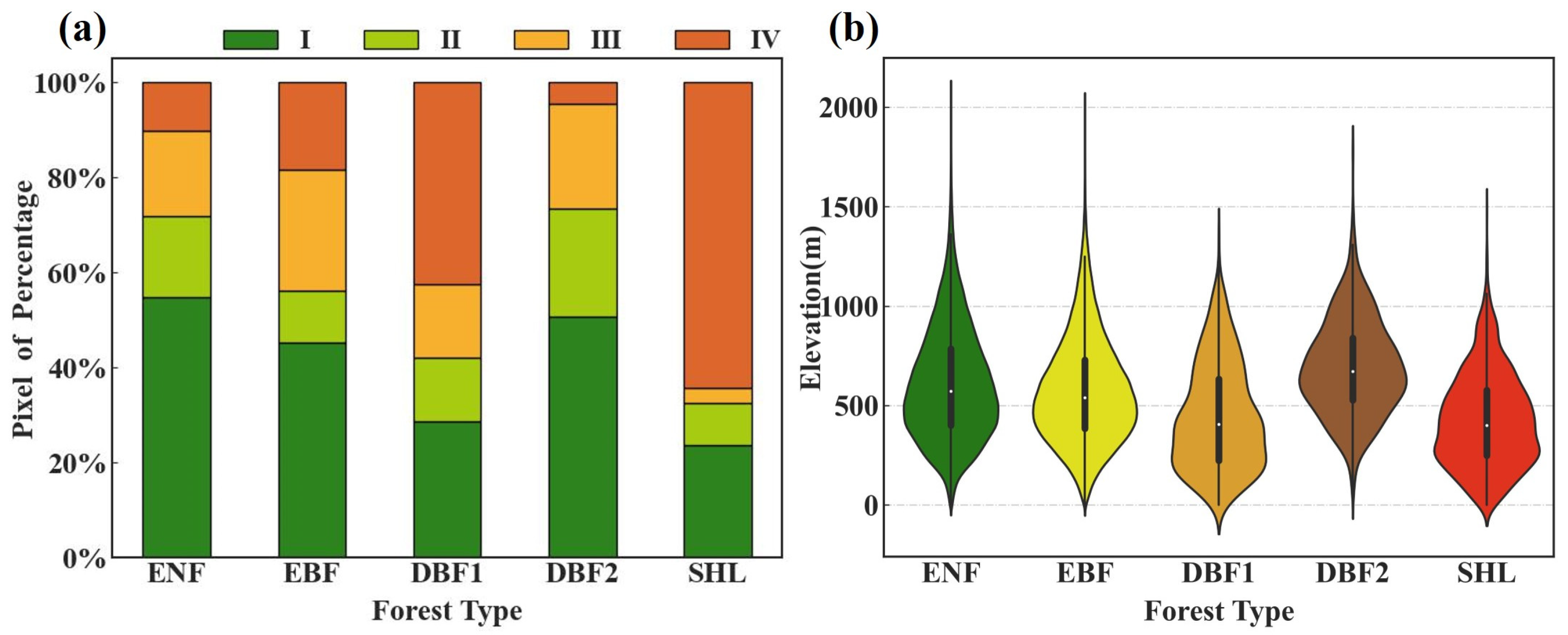
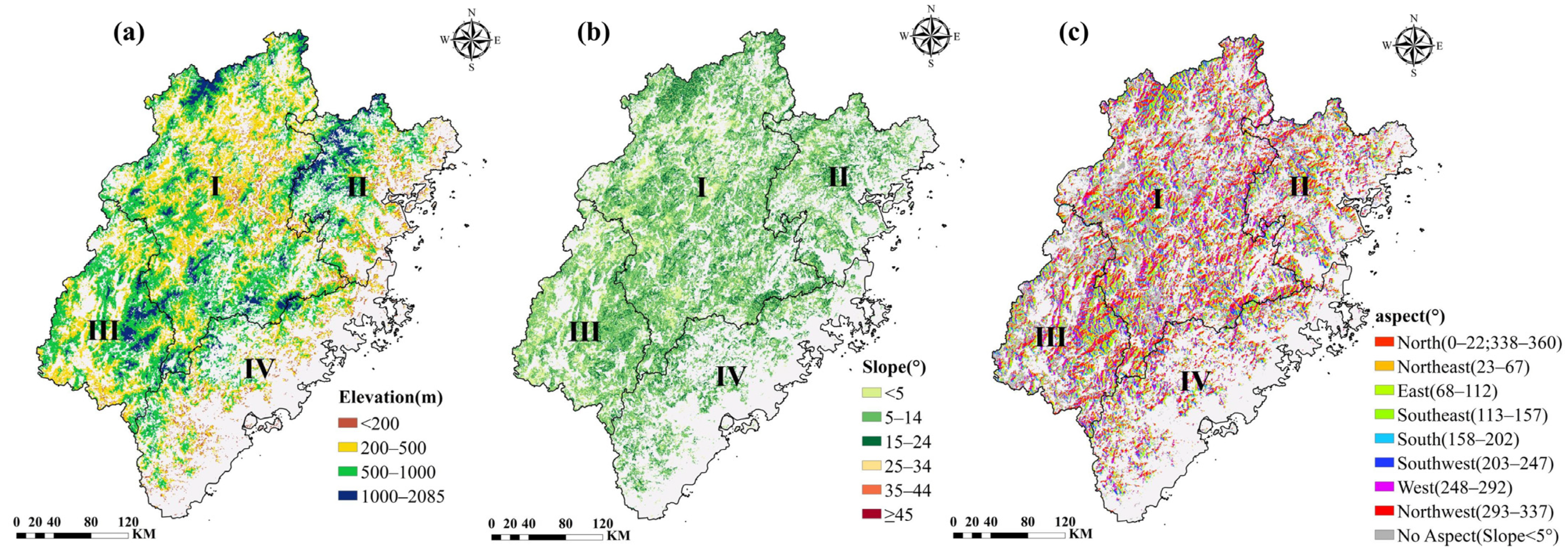
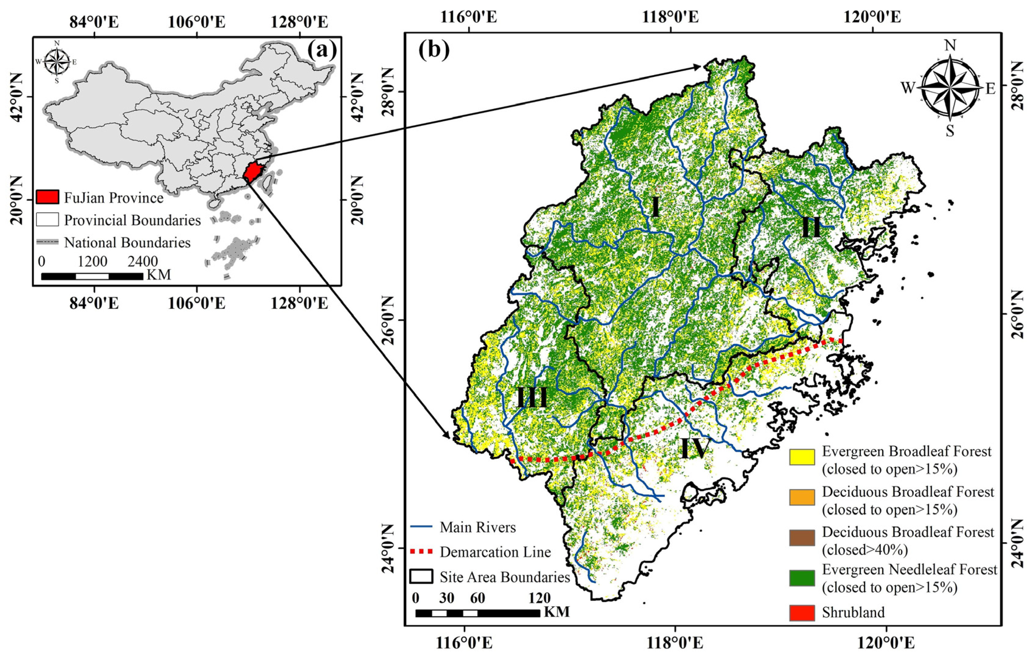
2.1. Study Area
2.2. Data and Preprocessing
2.2.1. Phenological Data
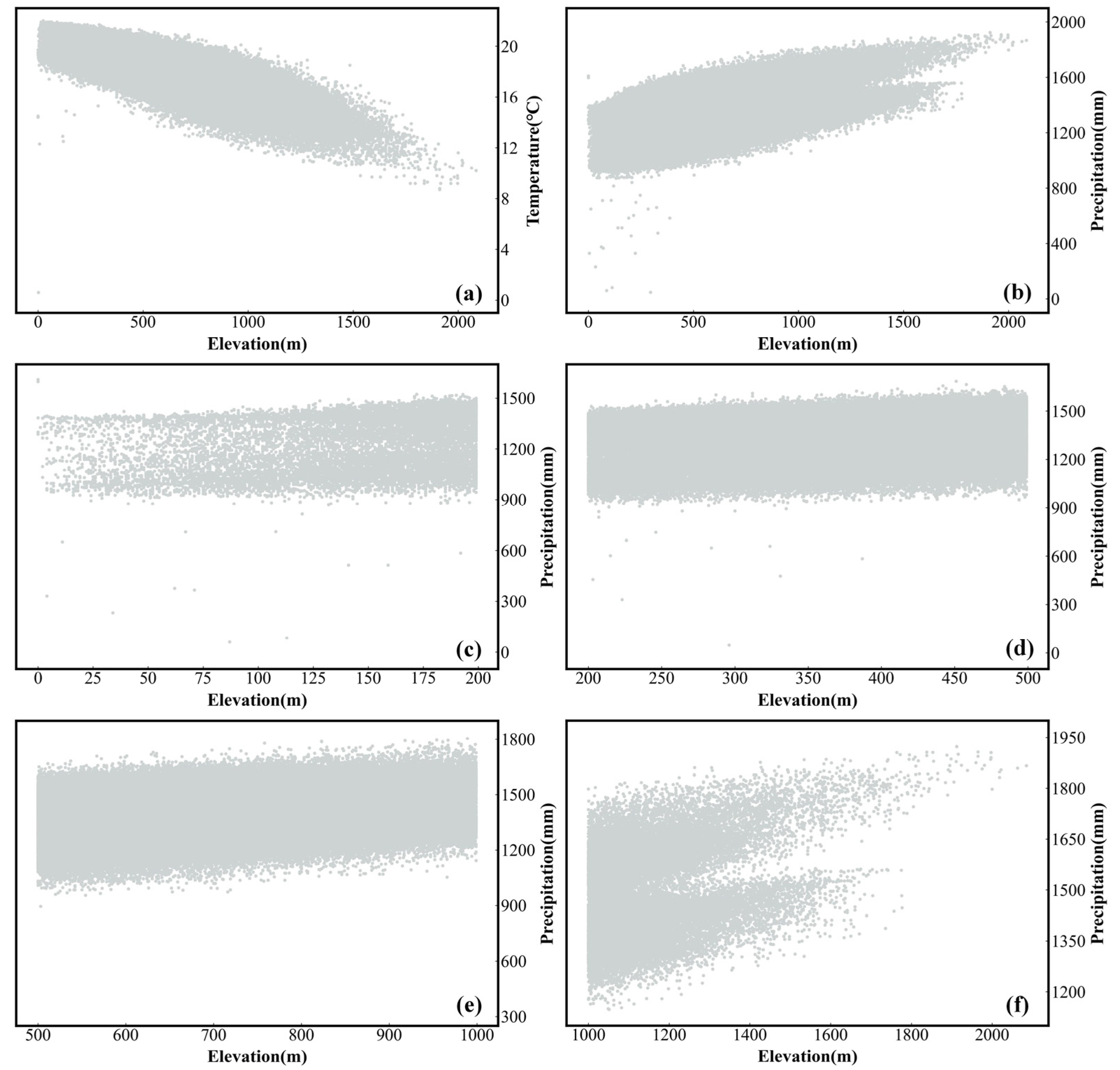
2.2.2. Thematic Data
2.3. Methods
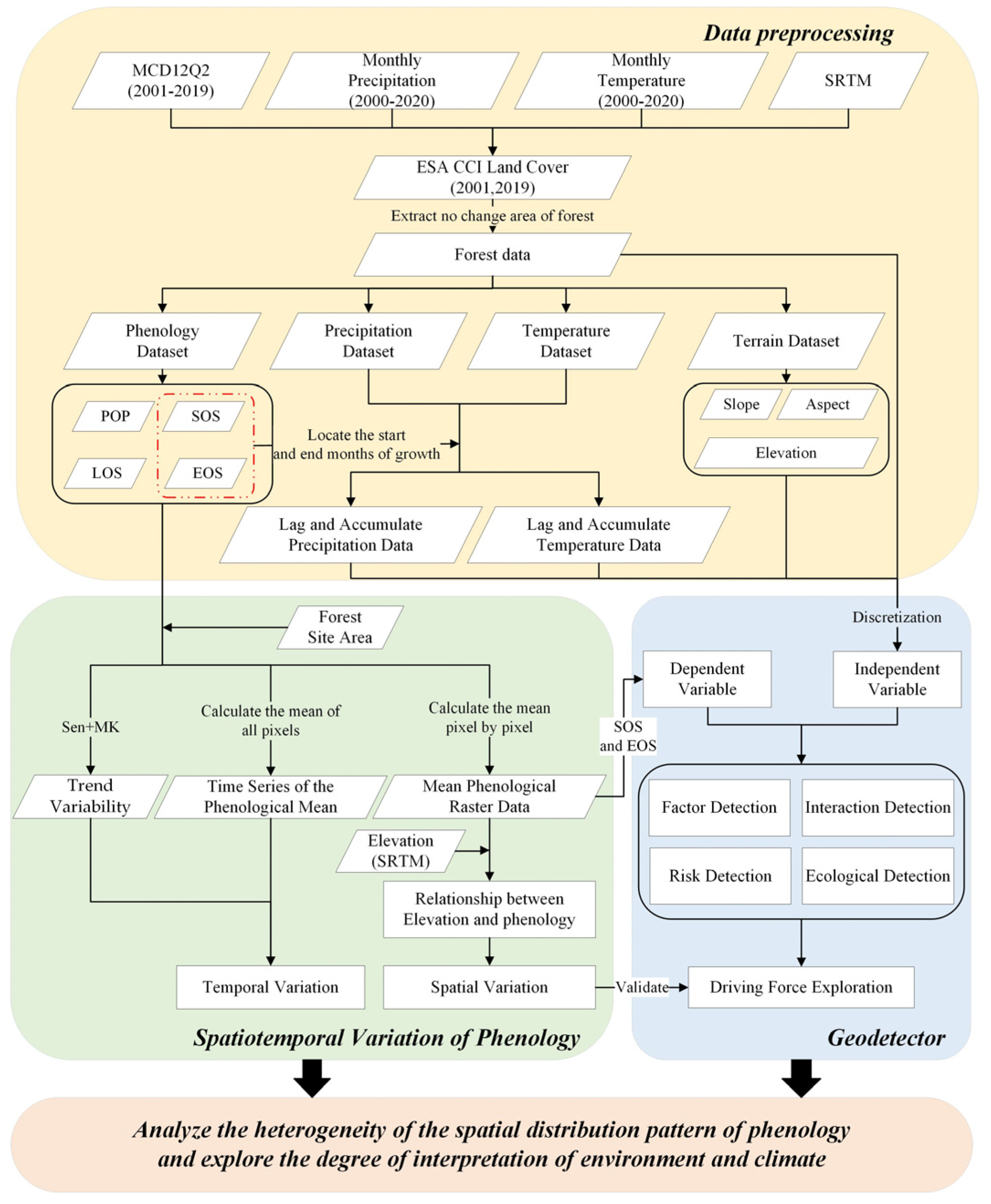
2.3.1. Workflow
2.3.2. Trend Analysis
2.3.3. GeoDetector
3. Results
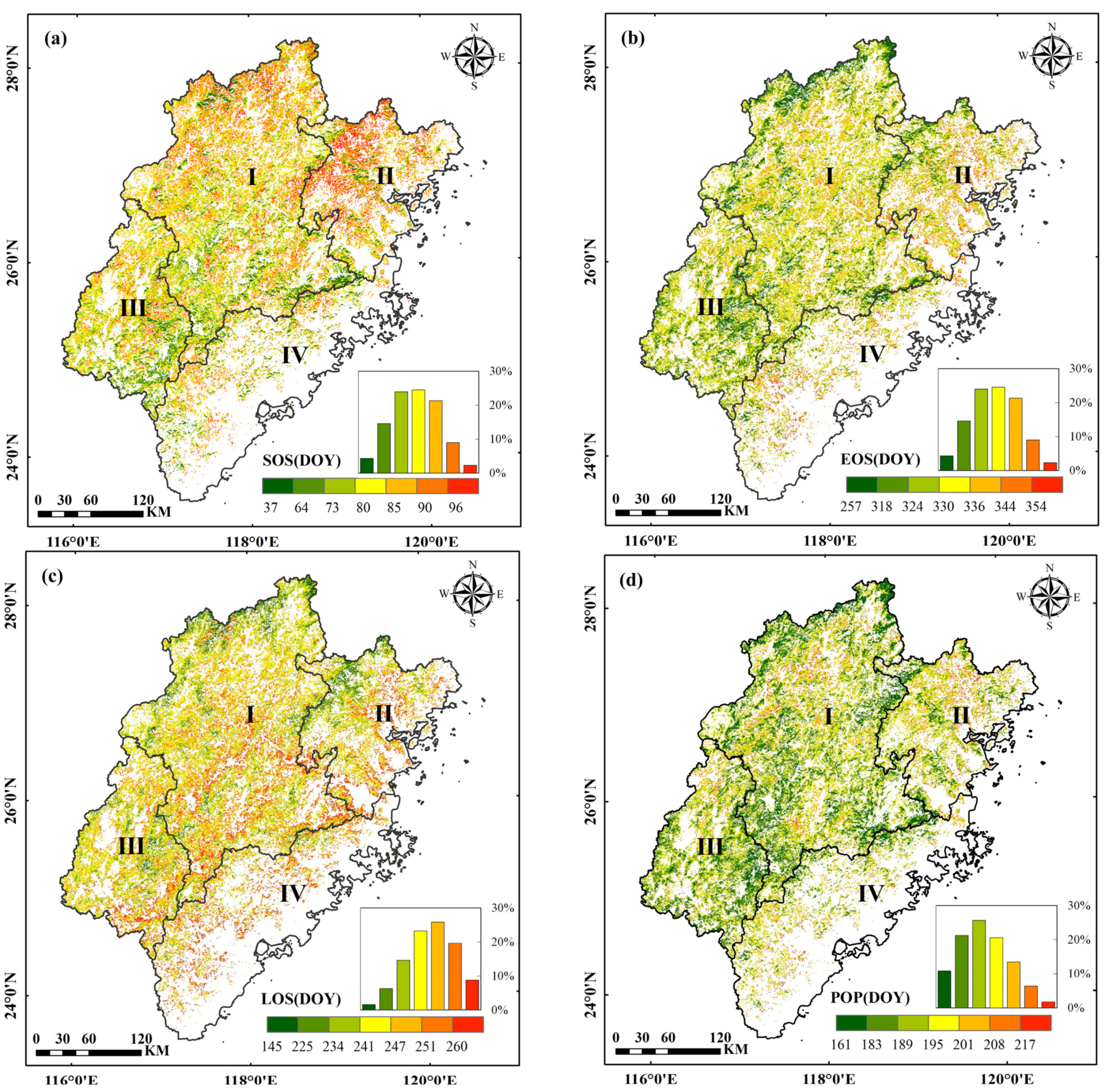
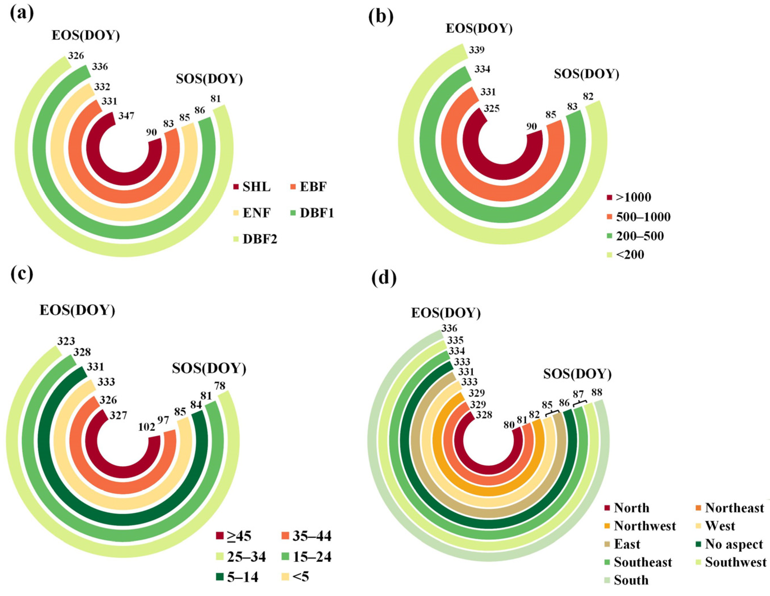
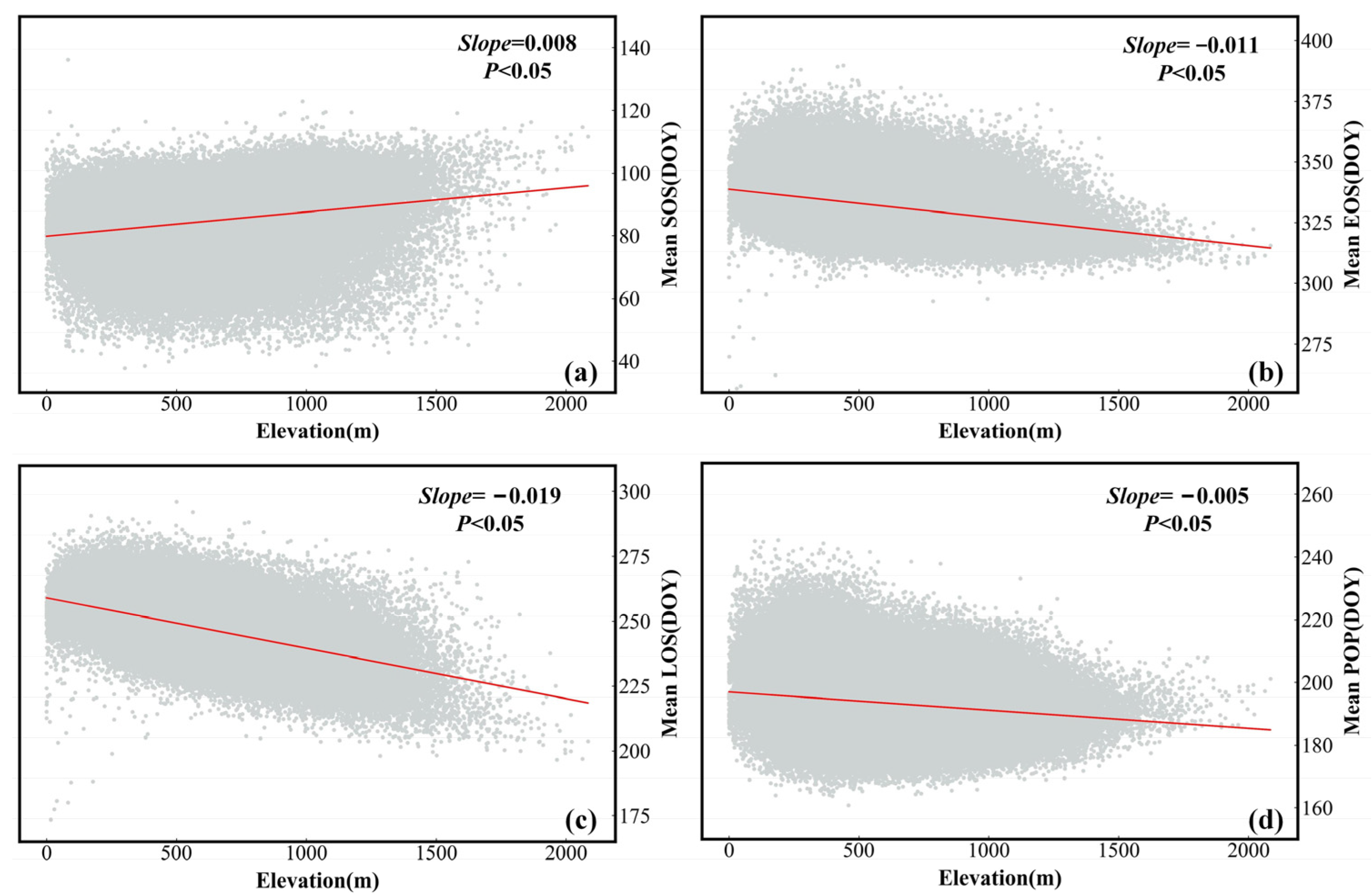
3.1. Spatial Pattern of the Phenological Parameters
3.2. Variation Trends of the Phenological Parameters
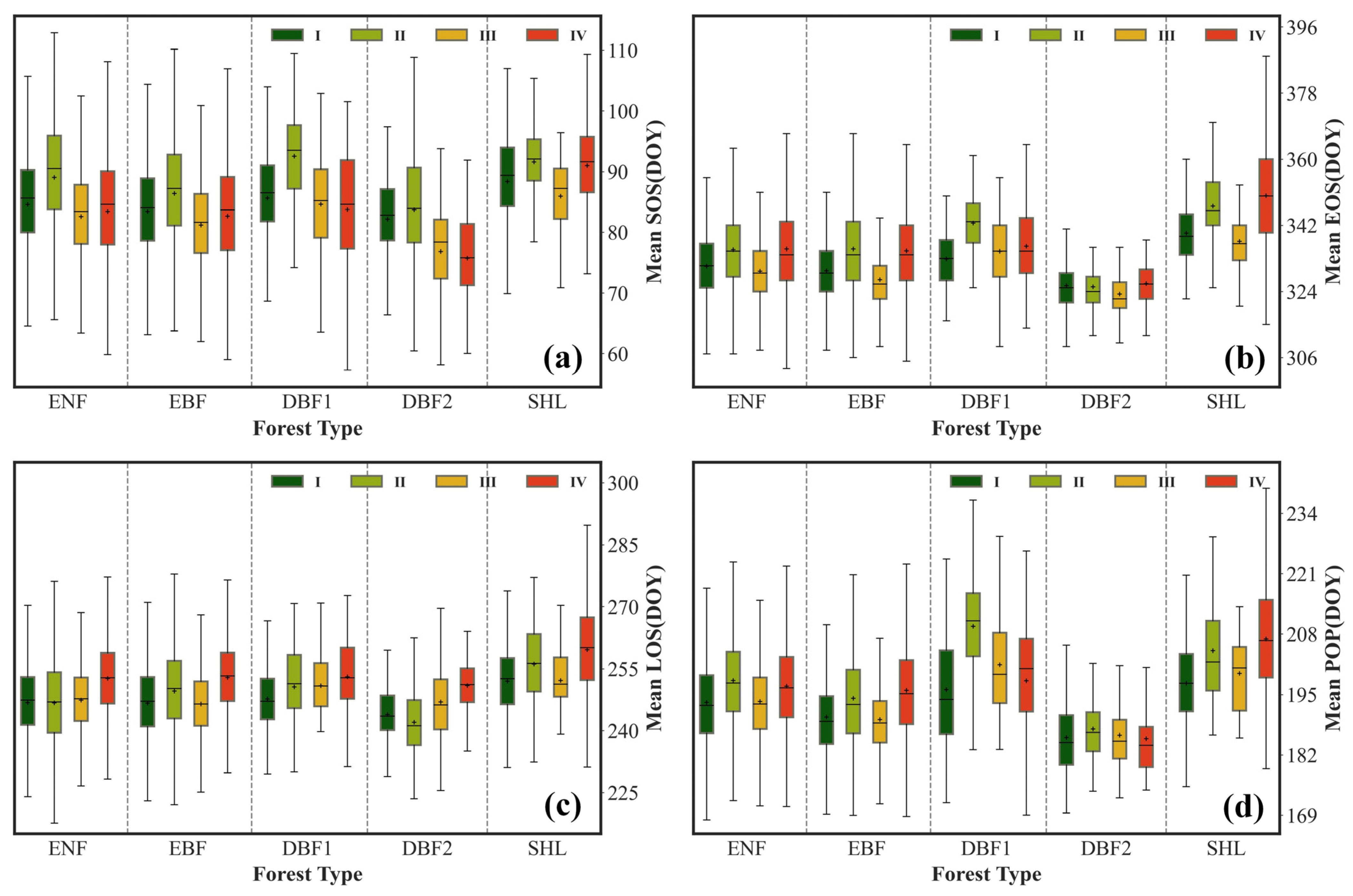
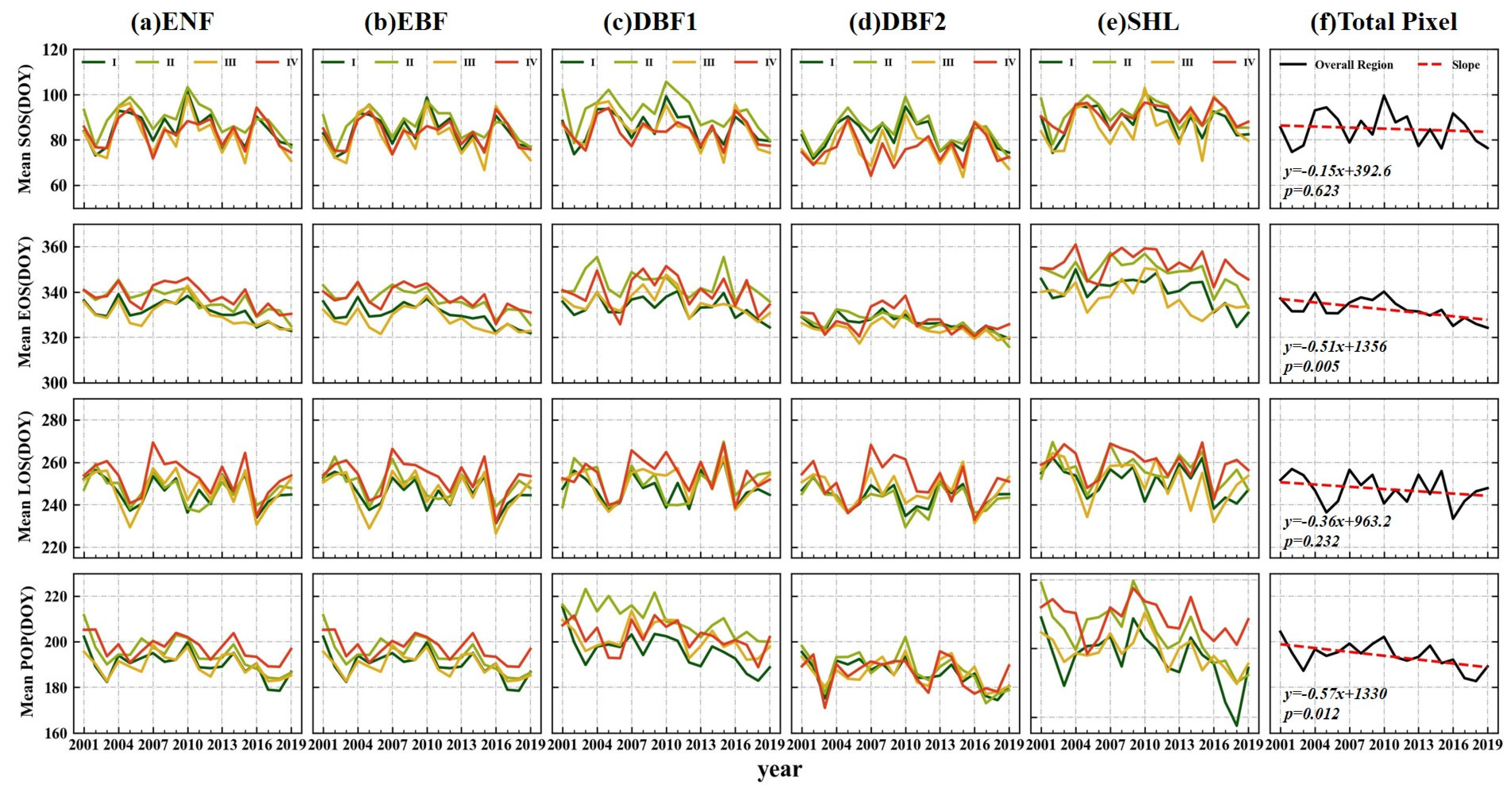
3.2.1. Temporal Variability of the Mean
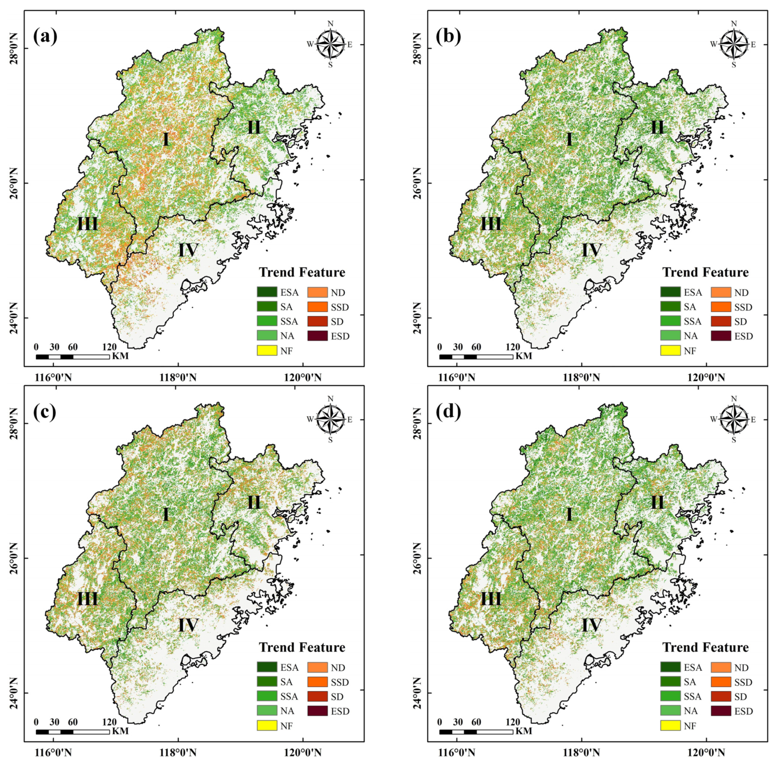
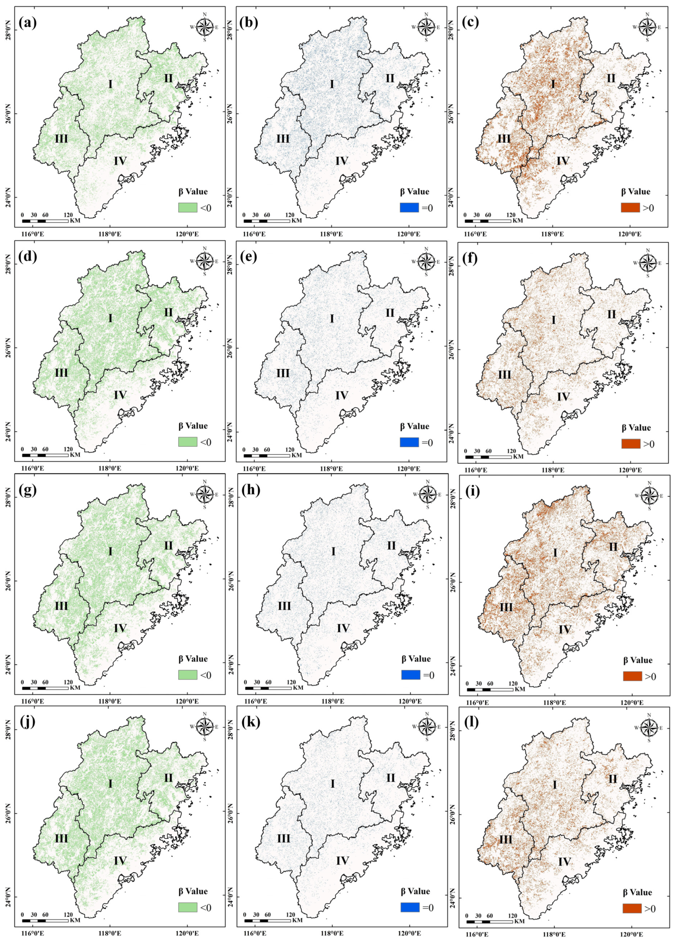
3.2.2. Variation Trends of the Regions
3.3. Exploration of the Driving Factors of SOS and EOS Spatial Differentiation
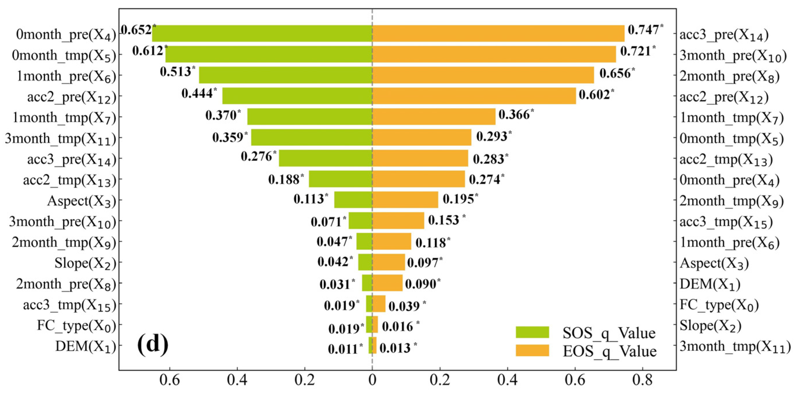
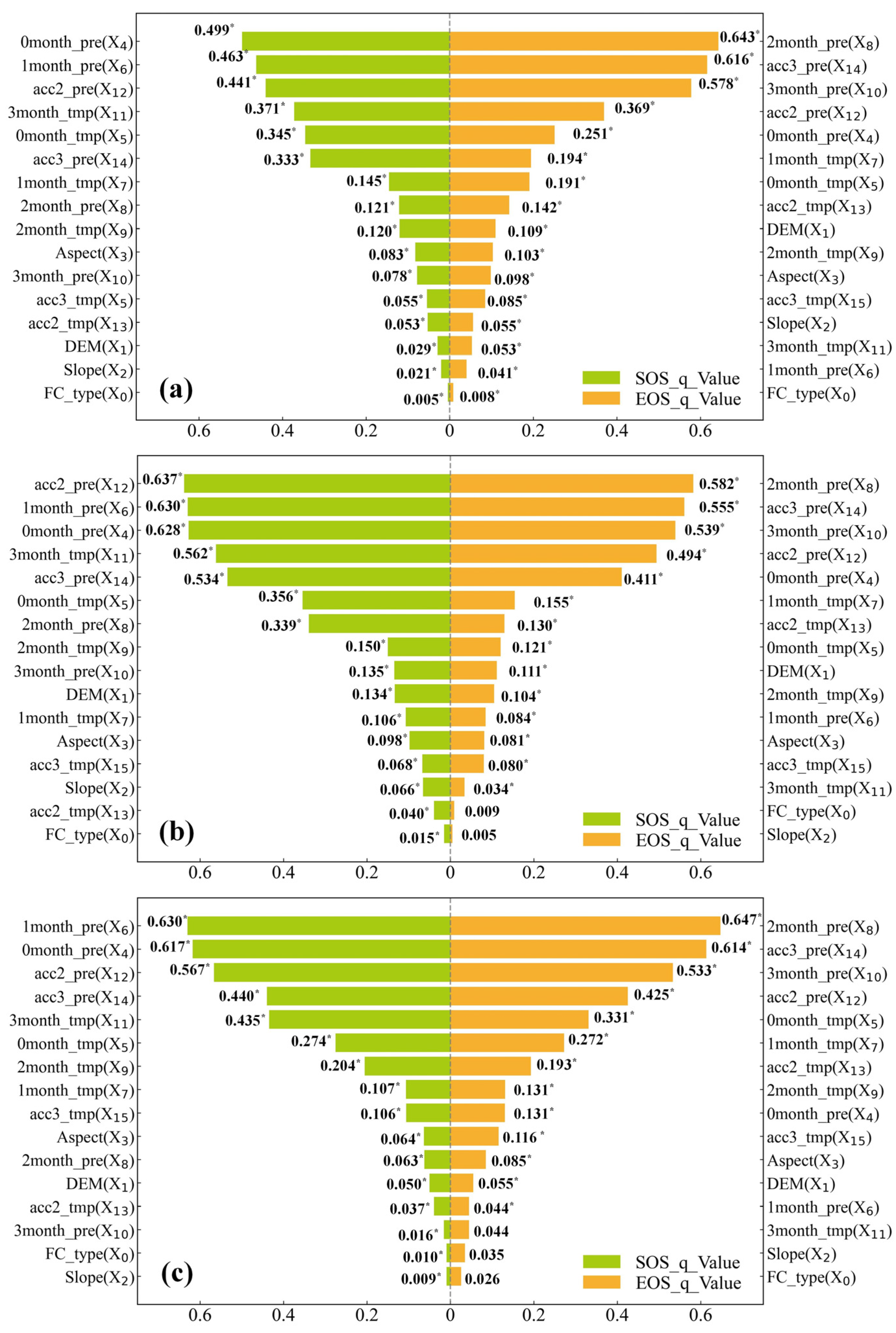
3.3.1. Single-Factor Exploration
3.3.2. Two-Factor Analysis
3.3.3. Interval Factor Detection
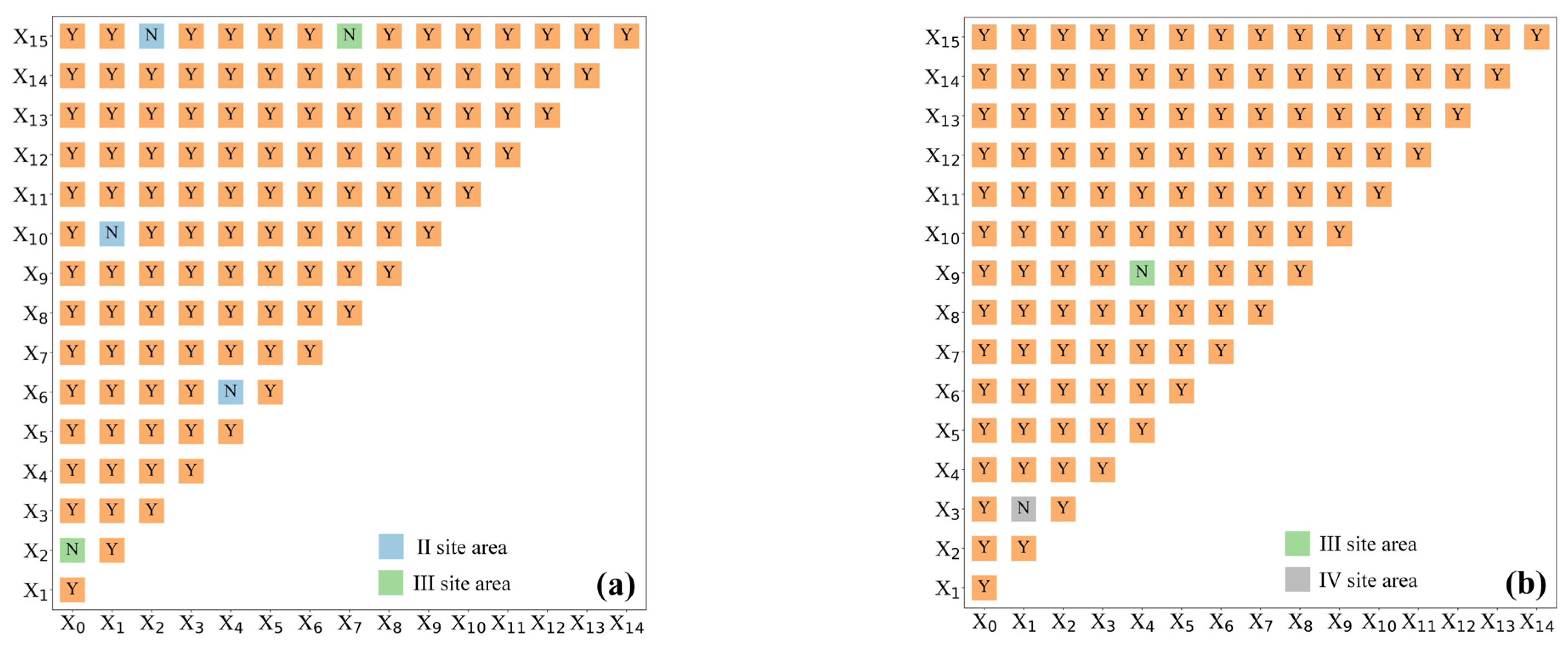
3.3.4. Significance Analysis of Factor Interactions
4. Discussion
4.1. Spatiotemporal Variation Characteristics of Forest Phenological Parameters
4.2. Exploration of the Drivers of the SOS and EOS
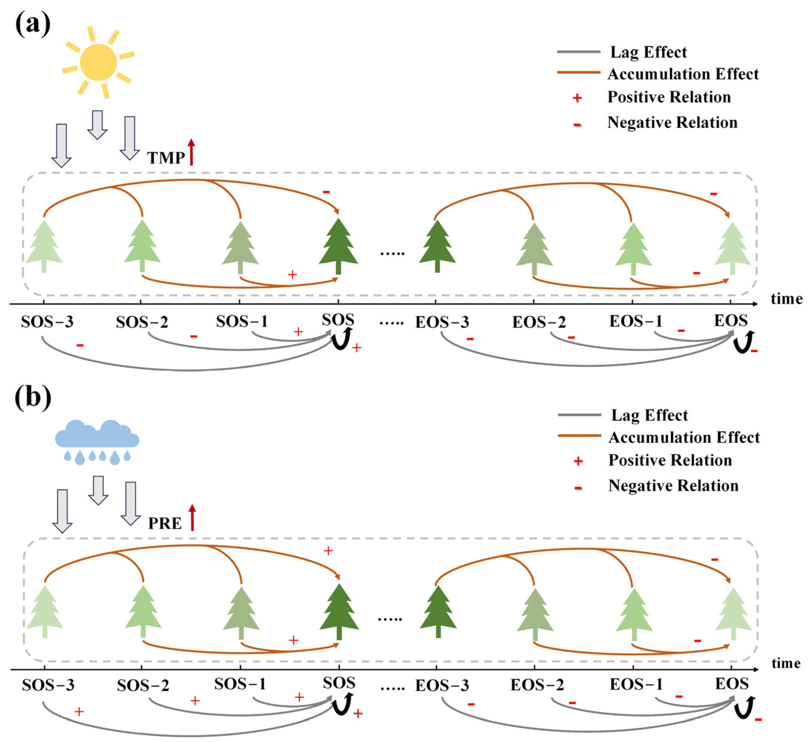
4.3. Effects of Factor-Driven Tree Physiological Processes on the SOS and EOS
4.4. Limitations and Uncertainties
5. Conclusions
Author Contributions
Funding
Data Availability Statement
Acknowledgments
Conflicts of Interest
Appendix A


References
- Chmielewski, F.-M.; Rötzer, T. Response of Tree Phenology to Climate Change across Europe. Agric. For. Meteorol. 2001, 108, 101–112. [Google Scholar] [CrossRef]
- Tan, J.; Piao, S.; Chen, A.; Zeng, Z.; Ciais, P.; Janssens, I.A.; Mao, J.; Myneni, R.B.; Peng, S.; Peñuelas, J.; et al. Seasonally Different Response of Photosynthetic Activity to Daytime and Night-Time Warming in the Northern Hemisphere. Glob. Chang. Biol. 2015, 21, 377–387. [Google Scholar] [CrossRef] [PubMed]
- Xia, H.; Qin, Y.; Feng, G.; Meng, Q.; Cui, Y.; Song, H.; Ouyang, Y.; Liu, G. Forest Phenology Dynamics to Climate Change and Topography in a Geographic and Climate Transition Zone: The Qinling Mountains in Central China. Forests 2019, 10, 1007. [Google Scholar] [CrossRef]
- Savitzky, A.; Golay, M.J.E. Smoothing and Differentiation of Data by Simplified Least Squares Procedures. Anal. Chem. 1964, 36, 1627–1639. [Google Scholar] [CrossRef]
- Jonsson, P.; Eklundh, L. Seasonality Extraction by Function Fitting to Time-Series of Satellite Sensor Data. IEEE Trans. Geosci. Remote Sens. 2002, 40, 1824–1832. [Google Scholar] [CrossRef]
- Beck, P.S.A.; Atzberger, C.; Høgda, K.A.; Johansen, B.; Skidmore, A.K. Improved Monitoring of Vegetation Dynamics at Very High Latitudes: A New Method Using MODIS NDVI. Remote Sens. Environ. 2006, 100, 321–334. [Google Scholar] [CrossRef]
- Klisch, A.; Atzberger, C. Evaluating Phenological Metrics Derived from the MODIS Time Series over the European Continent. Photogramm. Fernerkund. Geoinf. 2014, 5, 409–421. [Google Scholar] [CrossRef] [PubMed]
- White, M.A.; Thornton, P.E.; Running, S.W. A Continental Phenology Model for Monitoring Vegetation Responses to Interannual Climatic Variability. Glob. Biogeochem. Cycles 1997, 11, 217–234. [Google Scholar] [CrossRef]
- Reed, B.C.; Brown, J.F.; VanderZee, D.; Loveland, T.R.; Merchant, J.W.; Ohlen, D.O. Measuring Phenological Variability from Satellite Imagery. J. Veg. Sci. 1994, 5, 703–714. [Google Scholar] [CrossRef]
- Li, C.; Zhuang, D.; He, J.; Wen, K. Spatiotemporal Variations in Remote Sensing Phenology of Vegetation and Its Responses to Temperature Change of Boreal Forest in Tundra-Taiga Transitional Zone in the Eastern Siberia. J. Geogr. Sci. 2023, 33, 464–482. [Google Scholar] [CrossRef]
- Li, J.; Guan, J.; Han, W.; Tian, R.; Lu, B.; Yu, D.; Zheng, J. Important Role of Precipitation in Controlling a More Uniform Spring Phenology in the Qinba Mountains, China. Front. Plant Sci. 2023, 14, 1074405. [Google Scholar] [CrossRef] [PubMed]
- Yuan, M.; Zhao, L.; Lin, A.; Wang, L.; Li, Q.; She, D.; Qu, S. Impacts of Preseason Drought on Vegetation Spring Phenology across the Northeast China Transect. Sci. Total Environ. 2020, 738, 140297. [Google Scholar] [CrossRef] [PubMed]
- Zhou, X.; Geng, X.; Yin, G.; Hänninen, H.; Hao, F.; Zhang, X.; Fu, Y.H. Legacy Effect of Spring Phenology on Vegetation Growth in Temperate China. Agric. For. Meteorol. 2020, 281, 107845. [Google Scholar] [CrossRef]
- Zhu, W.; Zhang, X.; Zhang, J.; Zhu, L. A Comprehensive Analysis of Phenological Changes in Forest Vegetation of the Funiu Mountains, China. J. Geogr. Sci. 2019, 29, 131–145. [Google Scholar] [CrossRef]
- Piao, S.; Fang, J.; Ciais, P.; Peylin, P.; Huang, Y.; Sitch, S.; Wang, T. The Carbon Balance of Terrestrial Ecosystems in China. Nature 2009, 458, 1009–1013. [Google Scholar] [CrossRef] [PubMed]
- Yu, G.; Chen, Z.; Piao, S.; Peng, C.; Ciais, P.; Wang, Q.; Li, X.; Zhu, X. High Carbon Dioxide Uptake by Subtropical Forest Ecosystems in the East Asian Monsoon Region. Proc. Natl. Acad. Sci. USA 2014, 111, 4910–4915. [Google Scholar] [CrossRef] [PubMed]
- National Bureau of Statistics of China. China Statistical Yearbook; China Statistics Press: Beijing, China, 2022; ISBN 978-7-5037-9950-1.
- Xu, K.; Zeng, H.; Zhang, Z.; Xie, J.; Yang, Y. Remote sensing analysis of correlation between forest growing season and temperature and precipitation in subtropical Fujian Province. J. Geo-Inf. Sci. 2015, 17, 1249–1259. [Google Scholar]
- Niu, S.; Fu, Z.; Luo, Y.; Stoy, P.C.; Keenan, T.F.; Poulter, B.; Zhang, L.; Piao, S.; Zhou, X.; Zheng, H.; et al. Interannual Variability of Ecosystem Carbon Exchange: From Observation to Prediction. Glob. Ecol. Biogeogr. 2017, 26, 1225–1237. [Google Scholar] [CrossRef]
- Sun, H.; Chen, Y.; Xiong, J.; Ye, C.; Yong, Z.; Wang, Y.; He, D.; Xu, S. Relationships between Climate Change, Phenology, Edaphic Factors, and Net Primary Productivity across the Tibetan Plateau. Int. J. Appl. Earth Obs. Geoinf. 2022, 107, 102708. [Google Scholar] [CrossRef]
- Delpierre, N.; Vitasse, Y.; Chuine, I.; Guillemot, J.; Bazot, S.; Rutishauser, T.; Rathgeber, C.B.K. Temperate and Boreal Forest Tree Phenology: From Organ-Scale Processes to Terrestrial Ecosystem Models. Ann. For. Sci. 2016, 73, 5–25. [Google Scholar] [CrossRef]
- Li, X.; Fu, Y.H.; Chen, S.; Xiao, J.; Yin, G.; Li, X.; Zhang, X.; Geng, X.; Wu, Z.; Zhou, X.; et al. Increasing Importance of Precipitation in Spring Phenology with Decreasing Latitudes in Subtropical Forest Area in China. Agric. For. Meteorol. 2021, 304–305, 108427. [Google Scholar] [CrossRef]
- Fu, Y.H.; Zhao, H.; Piao, S.; Peaucelle, M.; Peng, S.; Zhou, G.; Ciais, P.; Huang, M.; Menzel, A.; Peñuelas, J.; et al. Declining Global Warming Effects on the Phenology of Spring Leaf Unfolding. Nature 2015, 526, 104–107. [Google Scholar] [CrossRef]
- Du, Y.; Pan, Y.; Ma, K. Moderate Chilling Requirement Controls Budburst for Subtropical Species in China. Agric. For. Meteorol. 2019, 278, 107693. [Google Scholar] [CrossRef]
- Park, J.Y.; Muller-Landau, H.C.; Lichstein, J.W.; Rifai, S.W.; Dandois, J.P.; Bohlman, S.A. Quantifying Leaf Phenology of Individual Trees and Species in a Tropical Forest Using Unmanned Aerial Vehicle (UAV) Images. Remote Sens. 2019, 11, 1534. [Google Scholar] [CrossRef]
- Song, Z.; Song, X.; Pan, Y.; Dai, K.; Shou, J.; Chen, Q.; Huang, J.; Tang, X.; Huang, Z.; Du, Y. Effects of Winter Chilling and Photoperiod on Leaf-out and Flowering in a Subtropical Evergreen Broadleaved Forest in China. For. Ecol. Manag. 2020, 458, 117766. [Google Scholar] [CrossRef]
- Li, Z.; Wang, R.; Liu, B.; Qian, Z.; Wu, Y.; Li, C. Responses of Vegetation Autumn Phenology to Climatic Factors in Northern China. Sustainability 2022, 14, 8590. [Google Scholar] [CrossRef]
- Yuan, Y.; Bao, A.; Jiapaer, G.; Jiang, L.; De Maeyer, P. Phenology-Based Seasonal Terrestrial Vegetation Growth Response to Climate Variability with Consideration of Cumulative Effect and Biological Carryover. Sci. Total Environ. 2022, 817, 152805. [Google Scholar] [CrossRef] [PubMed]
- Tang, W.; Liu, S.; Kang, P.; Peng, X.; Li, Y.; Guo, R.; Jia, J.; Liu, M.; Zhu, L. Quantifying the Lagged Effects of Climate Factors on Vegetation Growth in 32 Major Cities of China. Ecol. Indic. 2021, 132, 108290. [Google Scholar] [CrossRef]
- Liu, N.; Shi, Y.; Ding, Y.; Liu, L.; Peng, S. Temporal Effects of Climatic Factors on Vegetation Phenology on the Loess Plateau, China. J. Plant Ecol. 2023, 16, rtac063. [Google Scholar] [CrossRef]
- Wang, J.; Zhang, T.; Fu, B. A Measure of Spatial Stratified Heterogeneity. Ecol. Indic. 2016, 67, 250–256. [Google Scholar] [CrossRef]
- Wang, J.; Xu, C. Geodetectors: Principles and prospects. Acta Geogr. Sin. 2017, 72, 116–134. [Google Scholar] [CrossRef]
- Luo, L.; Mei, K.; Qu, L.; Zhang, C.; Chen, H.; Wang, S.; Di, D.; Huang, H.; Wang, Z.; Xia, F.; et al. Assessment of the Geographical Detector Method for Investigating Heavy Metal Source Apportionment in an Urban Watershed of Eastern China. Sci. Total Environ. 2019, 653, 714–722. [Google Scholar] [CrossRef]
- Li, C.; Zou, Y.; He, J.; Zhang, W.; Gao, L.; Zhuang, D. Response of Vegetation Phenology to the Interaction of Temperature and Precipitation Changes in Qilian Mountains. Remote Sens. 2022, 14, 1248. [Google Scholar] [CrossRef]
- Peng, H.; Xia, H.; Chen, H.; Zhi, P.; Xu, Z. Spatial Variation Characteristics of Vegetation Phenology and Its Influencing Factors in the Subtropical Monsoon Climate Region of Southern China. PLoS ONE 2021, 16, e0250825. [Google Scholar] [CrossRef]
- Sun, Y.; Guan, Q.; Wang, Q.; Yang, L.; Pan, N.; Ma, Y.; Luo, H. Quantitative Assessment of the Impact of Climatic Factors on Phenological Changes in the Qilian Mountains, China. For. Ecol. Manag. 2021, 499, 119594. [Google Scholar] [CrossRef]
- Yang, C.; Deng, K.; Peng, D.; Jiang, L.; Zhao, M.; Liu, J.; Qiu, X. Spatiotemporal Characteristics and Heterogeneity of Vegetation Phenology in the Yangtze River Delta. Remote Sens. 2022, 14, 2984. [Google Scholar] [CrossRef]
- Zhan, Z. (Ed.) Forest Site Types in China; China Forestry Publishing: Beijing, China, 1995; ISBN 978-7-5038-1484-6. [Google Scholar]
- Yang, Q.; Zheng, D.; Wu, S. Study on ecological areal system in China. Prog. Nat. Sci. 2002, 12, 65–69. [Google Scholar] [CrossRef]
- Gray, J.; Sulla-Menashe, D.; Friedl, M.A. User Guide to Collection 6 MODIS Land Cover Dynamics (MCD12Q2) Product; NASA EOSDIS Land Processes DAAC: Missoula, MT, USA, 2019. [Google Scholar]
- Ganguly, S.; Friedl, M.A.; Tan, B.; Zhang, X.; Verma, M. Land Surface Phenology from MODIS: Characterization of the Collection 5 Global Land Cover Dynamics Product. Remote Sens. Environ. 2010, 114, 1805–1816. [Google Scholar] [CrossRef]
- Peng, D.; Zhang, X.; Wu, C.; Huang, W.; Gonsamo, A.; Huete, A.R.; Didan, K.; Tan, B.; Liu, X.; Zhang, B. Intercomparison and Evaluation of Spring Phenology Products Using National Phenology Network and AmeriFlux Observations in the Contiguous United States. Agric. For. Meteorol. 2017, 242, 33–46. [Google Scholar] [CrossRef]
- Zhang, J.; Tong, X.; Zhang, J.; Meng, P.; Li, J.; Liu, P. Dynamics of Phenology and Its Response to Climatic Variables in a Warm-Temperate Mixed Plantation. For. Ecol. Manag. 2021, 483, 118785. [Google Scholar] [CrossRef]
- Purdy, L.M.; Sang, Z.; Beaubien, E.; Hamann, A. Validating Remotely Sensed Land Surface Phenology with Leaf out Records from a Citizen Science Network. Int. J. Appl. Earth Obs. Geoinf. 2023, 116, 103148. [Google Scholar] [CrossRef]
- Yang, L.; Wu, B.; Ma, J. Response of plant phenology to climate change in Fujian province. Chin. Agric. Sci. Bull. 2016, 32, 139–150. [Google Scholar] [CrossRef]
- Yang, H.; Xiao, P.; Feng, X.; Li, H. Accuracy Assessment of Seven Global Land Cover Datasets over China. ISPRS J. Photogramm. Remote Sens. 2017, 125, 156–173. [Google Scholar] [CrossRef]
- Peng, S.; Ding, Y.; Liu, W.; Li, Z. 1km Monthly Temperature and Precipitation Dataset for China from 1901 to 2017. Earth Syst. Sci. Data 2019, 11, 1931–1946. [Google Scholar] [CrossRef]
- Li, B.; Pan, B.; Han, J. Discussion on basic landform types and their classification indexes in China. Quat. Sci. 2008, 28, 535–543. [Google Scholar]
- Kendall, M.G. Rank Correlation Methods; Griffin: Oxford, UK, 1948; ISBN 0-19-520837-4. [Google Scholar]
- Tošić, I. Spatial and Temporal Variability of Winter and Summer Precipitation over Serbia and Montenegro. Theor. Appl. Clim. 2004, 77, 47–56. [Google Scholar] [CrossRef]
- Shi, S.; Wang, X.; Hu, Z.; Zhao, X.; Zhang, S.; Hou, M.; Zhang, N. Geographic Detector-Based Quantitative Assessment Enhances Attribution Analysis of Climate and Topography Factors to Vegetation Variation for Spatial Heterogeneity and Coupling. Glob. Ecol. Conserv. 2023, 42, e02398. [Google Scholar] [CrossRef]
- Jia, L.; Yu, K.; Li, Z.; Ren, Z.; Li, H.; Li, P. Identification of Vegetation Coverage Variation and Quantitative the Impact of Environmental Factors on Its Spatial Distribution in the Pisha Sandstone Area. Sustainability 2023, 15, 6054. [Google Scholar] [CrossRef]
- Zhang, Y.; Liu, X.; Jiao, W.; Wu, X.; Zeng, X.; Zhao, L.; Wang, L.; Guo, J.; Xing, X.; Hong, Y. Spatial Heterogeneity of Vegetation Resilience Changes to Different Drought Types. Earth’s Future 2023, 11, e2022EF003108. [Google Scholar] [CrossRef]
- Wang, M.; Wang, Y.; Li, Z.; Zhang, H. Analysis of Spatial-Temporal Changes and Driving Factors of Vegetation Coverage in Jiamusi City. Forests 2023, 14, 1902. [Google Scholar] [CrossRef]
- Song, Y.; Wang, J.; Ge, Y.; Xu, C. An Optimal Parameters-Based Geographical Detector Model Enhances Geographic Characteristics of Explanatory Variables for Spatial Heterogeneity Analysis: Cases with Different Types of Spatial Data. GIScience Remote Sens. 2020, 57, 593–610. [Google Scholar] [CrossRef]
- R Core Team. R: A Language and Environment for Statistical Computing; R Foundation Statistical Computing: Vienna, Austria, 2022. [Google Scholar]
- Wen, Y.; Liu, X.; Xin, Q.; Wu, J.; Xu, X.; Pei, F.; Li, X.; Du, G.; Cai, Y.; Lin, K.; et al. Cumulative Effects of Climatic Factors on Terrestrial Vegetation Growth. J. Geophys. Res. Biogeosci. 2019, 124, 789–806. [Google Scholar] [CrossRef]
- Wu, D.; Zhao, X.; Liang, S.; Zhou, T.; Huang, K.; Tang, B.; Zhao, W. Time-Lag Effects of Global Vegetation Responses to Climate Chang. Glob. Chang. Biol. 2015, 21, 3520–3531. [Google Scholar] [CrossRef] [PubMed]
- Qiu, B.; Zhong, M.; Tang, Z.; Chen, C. Spatiotemporal Variability of Vegetation Phenology with Reference to Altitude and Climate in the Subtropical Mountain and Hill Region, China. Chin. Sci. Bull. 2013, 58, 2883–2892. [Google Scholar] [CrossRef]
- Zhang, Y.; Yin, P.; Li, X.; Niu, Q.; Wang, Y.; Cao, W.; Huang, J.; Chen, H.; Yao, X.; Yu, L.; et al. The Divergent Response of Vegetation Phenology to Urbanization: A Case Study of Beijing City, China. Sci. Total Environ. 2022, 803, 150079. [Google Scholar] [CrossRef] [PubMed]
- Colditz, R.R.; Lopez, G.; Maeda, P.; Cruz, I.; Ressl, R. Phenology and Phenological Variability of Mexican Ecosystems. In Proceedings of the 2009 IEEE International Geoscience and Remote Sensing Symposium, Cape Town, South Africa, 12–17 July 2009; pp. IV-1038–IV-1041. [Google Scholar]
- Wang, H.; Wang, H.; Ge, Q.; Dai, J. The Interactive Effects of Chilling, Photoperiod, and Forcing Temperature on Flowering Phenology of Temperate Woody Plants. Front. Plant Sci. 2020, 11, 443. [Google Scholar] [CrossRef] [PubMed]
- Mendoza, I.; Peres, C.A.; Morellato, L.P.C. Continental-Scale Patterns and Climatic Drivers of Fruiting Phenology: A Quantitative Neotropical Review. Glob. Planet. Chang. 2017, 148, 227–241. [Google Scholar] [CrossRef]
- Ren, P.; Liu, Z.; Zhou, X.; Peng, C.; Xiao, J.; Wang, S.; Li, X.; Li, P. Strong Controls of Daily Minimum Temperature on the Autumn Photosynthetic Phenology of Subtropical Vegetation in China. For. Ecosyst. 2021, 8, 31. [Google Scholar] [CrossRef]
- Ge, C.; Sun, S.; Yao, R.; Sun, P.; Li, M.; Bian, Y. Long-Term Vegetation Phenology Changes and Response to Multi-Scale Meteorological Drought on the Loess Plateau, China. J. Hydrol. 2022, 614, 128605. [Google Scholar] [CrossRef]
- De Frenne, P.; Lenoir, J.; Luoto, M.; Scheffers, B.R.; Zellweger, F.; Aalto, J.; Ashcroft, M.B.; Christiansen, D.M.; Decocq, G.; De Pauw, K.; et al. Forest Microclimates and Climate Change: Importance, Drivers and Future Research Agenda. Glob. Chang. Biol. 2021, 27, 2279–2297. [Google Scholar] [CrossRef]
- Davidson, E.A.; de Araújo, A.C.; Artaxo, P.; Balch, J.K.; Brown, I.F.; Bustamante, M.M.C.; Coe, M.T.; DeFries, R.S.; Keller, M.; Longo, M.; et al. The Amazon Basin in Transition. Nature 2012, 481, 321–328. [Google Scholar] [CrossRef]
- Brando, P.M.; Goetz, S.J.; Baccini, A.; Nepstad, D.C.; Beck, P.S.A.; Christman, M.C. Seasonal and Interannual Variability of Climate and Vegetation Indices across the Amazon. Proc. Natl. Acad. Sci. USA 2010, 107, 14685–14690. [Google Scholar] [CrossRef]
- Shen, M.; Piao, S.; Cong, N.; Zhang, G.; Jassens, I.A. Precipitation Impacts on Vegetation Spring Phenology on the Tibetan Plateau. Glob. Chang. Biol. 2015, 21, 3647–3656. [Google Scholar] [CrossRef] [PubMed]
- Lang, G.A.; Early, J.D.; Martin, G.C.; Darnell, R.L. Endo-, Para-, and Ecodormancy: Physiological Terminology and Classification for Dormancy Research. HortScience 1987, 22, 371–377. [Google Scholar] [CrossRef]
- Chuine, I.; Bonhomme, M.; Legave, J.-M.; García de Cortázar-Atauri, I.; Charrier, G.; Lacointe, A.; Améglio, T. Can Phenological Models Predict Tree Phenology Accurately in the Future? The Unrevealed Hurdle of Endodormancy Break. Glob. Chang. Biol. 2016, 22, 3444–3460. [Google Scholar] [CrossRef] [PubMed]
- Garrigues, R.; Dox, I.; Flores, O.; Marchand, L.J.; Malyshev, A.V.; Beemster, G.; AbdElgawad, H.; Janssens, I.; Asard, H.; Campioli, M. Late Autumn Warming Can Both Delay and Advance Spring Budburst through Contrasting Effects on Bud Dormancy Depth in Fagus sylvatica L. Tree Physiol. 2023, 43, tpad080. [Google Scholar] [CrossRef] [PubMed]
- Li, J.; Huang, J.-G.; Tardif, J.C.; Liang, H.; Jiang, S.; Zhu, H.; Zhou, P. Spatially Heterogeneous Responses of Tree Radial Growth to Recent El Niño Southern-Oscillation Variability across East Asia Subtropical Forests. Agric. For. Meteorol. 2020, 287, 107939. [Google Scholar] [CrossRef]
- Prior, L.D.; Bowman, D.M.J.S.; Eamus, D. Seasonal Differences in Leaf Attributes in Australian Tropical Tree Species: Family and Habitat Comparisons. Funct. Ecol. 2004, 18, 707–718. [Google Scholar] [CrossRef]
- Gong, F.; Chen, X.; Yuan, W.; Su, Y.; Yang, X.; Liu, L.; Sun, Q.; Wu, J.; Dai, Y.; Shang, J. Partitioning of Three Phenology Rhythms in American Tropical and Subtropical Forests Using Remotely Sensed Solar-Induced Chlorophyll Fluorescence and Field Litterfall Observations. Int. J. Appl. Earth Obs. Geoinf. 2022, 107, 102698. [Google Scholar] [CrossRef]
- Cong, N.; Wang, T.; Nan, H.; Ma, Y.; Wang, X.; Myneni, R.B.; Piao, S. Changes in Satellite-Derived Spring Vegetation Green-up Date and Its Linkage to Climate in China from 1982 to 2010: A Multimethod Analysis. Glob. Chang. Biol. 2013, 19, 881–891. [Google Scholar] [CrossRef]


| Trend Significance Classification | ||
|---|---|---|
| Extremely significantly delayed | ||
| Significantly delayed | ||
| Slightly significantly delayed | ||
| Not significantly delayed | ||
| No fluctuations | ||
| Not significantly advanced | ||
| Slightly significantly advanced | ||
| Significantly advanced | ||
| Extremely significantly advanced |
| Factor | Description | Value Range | Unit |
|---|---|---|---|
| X0 | Forest type | ENF; EBF; DBF1; DBF2; SHL | \ |
| X1 | Elevation data | [0, 2085] | m |
| X2 | Slope data | [0, 50.4] | |
| X3 | Aspect data | [−1.0, 360.0) | |
| X4 | Monthly average precipitation | (175.9, 2711.7] | 0.1 mm |
| X5 | Monthly average air temperature | (3.2, 22.6] | °C |
| X6 | Monthly average precipitation in the previous month | (174.1, 1972.5] | 0.1 mm |
| X7 | Monthly average temperature in the previous month | (1.6, 24.4] | °C |
| X8 | Monthly average precipitation two months ago | (248.8, 2488.7] | 0.1 mm |
| X9 | Monthly average temperature two months ago | (0.4, 27.0] | °C |
| X10 | Monthly average precipitation three months ago | (182.8, 3241.7] | 0.1 mm |
| X11 | Monthly average temperature three months ago | (−0.1, 28.4] | °C |
| X12 | Accumulated average precipitation in the past two months | (266.7, 1789.4] | 0.1 mm |
| X13 | Accumulated average temperature in the past two months | (1.5, 25.7] | °C |
| X14 | Accumulated average precipitation in the past three months | (308.8, 2083.5] | 0.1 mm |
| X15 | Accumulated average temperature in the past three months | (1.2, 26.4] | °C |
| Interaction Types | Judgement Criteria |
|---|---|
| Nonlinear weakened | |
| Univariate weakened | |
| Bivariate enhanced | |
| Independent | |
| Nonlinear enhanced |
| Period | Site Area | ESA | SA | SSA | NA | NF | ND | SSD | SD | ESD | Trend | ENF | EBF | DBF1 | DBF2 | SHL |
|---|---|---|---|---|---|---|---|---|---|---|---|---|---|---|---|---|
| SOS | I | 28% | 31% | 36% | 51% | 59% | 58% | 54% | 47% | 32% | Advance | 66% | 60% | 72% | 65% | 51% |
| II | 40% | 42% | 36% | 19% | 13% | 8% | 4% | 3% | 2% | |||||||
| III | 9% | 12% | 16% | 21% | 19% | 23% | 16% | 14% | 11% | Delay | 34% | 40% | 28% | 35% | 49% | |
| IV | 23% | 15% | 12% | 9% | 9% | 13% | 26% | 36% | 55% | |||||||
| EOS | I | 54% | 54% | 55% | 54% | 55% | 50% | 45% | 44% | 45% | Advance | 80% | 78% | 66% | 76% | 61% |
| II | 26% | 23% | 20% | 16% | 12% | 10% | 8% | 7% | 5% | |||||||
| III | 13% | 15% | 16% | 20% | 23% | 25% | 28% | 29% | 23% | Delay | 20% | 22% | 34% | 24% | 39% | |
| IV | 7% | 8% | 9% | 11% | 10% | 15% | 19% | 20% | 29% | |||||||
| LOS | I | 65% | 61% | 59% | 54% | 53% | 48% | 47% | 46% | 51% | Advance | 68% | 69% | 53% | 66% | 64% |
| II | 16% | 16% | 16% | 15% | 17% | 16% | 18% | 19% | 18% | |||||||
| III | 11% | 14% | 15% | 20% | 21% | 24% | 23% | 22% | 20% | Delay | 32% | 31% | 47% | 34% | 36% | |
| IV | 8% | 9% | 10% | 11% | 10% | 12% | 12% | 13% | 10% | |||||||
| POP | I | 54% | 56% | 57% | 55% | 54% | 48% | 41% | 37% | 40% | Advance | 77% | 72% | 74% | 78% | 67% |
| II | 28% | 23% | 20% | 16% | 13% | 11% | 9% | 8% | 8% | |||||||
| III | 11% | 13% | 14% | 19% | 23% | 27% | 33% | 35% | 34% | Delay | 23% | 28% | 26% | 22% | 22% | |
| IV | 7% | 8% | 9% | 10% | 11% | 14% | 16% | 19% | 17% |
| Period | Site Area | Factor Interaction Ranking |
|---|---|---|
| SOS | I | X11∩X5 (0.782) ↑ > X15∩X5 (0.730) ↑ > X9∩X5 (0.718) ↑ > X6∩X5 (0.711) ↑↑ > X12∩X5 (0.700) ↑↑ |
| II | X11∩X5 (0.854) ↑↑ > X12∩X5 (0.849) ↑↑ > X6∩X5 (0.831) ↑↑ > X12∩X7 (0.828) ↑ > X14∩X5 (0.819) ↑↑ | |
| III | X11∩X5 (0.766) ↑ > X11∩X4 (0.739) ↑↑ > X6∩X5 (0.736) ↑↑ > X5∩X4 (0.729) ↑↑ > X15∩X5 (0.728) ↑ | |
| IV | X5∩X4 (0.856) ↑↑ > X7∩X4 (0.827) ↑↑ = X12∩X5 (0.827) ↑↑ > X6∩X5 (0.816) ↑↑ > X13∩X4 (0.811) ↑↑ | |
| EOS | I | X14∩X13 (0.839) ↑ > X14∩X9 (0.836) ↑ > X15∩X14 (0.834) ↑ > X14∩X7 (0.827) ↑ > X8∩X7 (0.804) ↑↑ |
| II | X14∩X7 (0.754) ↑ > X14∩X13 (0.747) ↑ > X14∩X9 (0.735) ↑ > X14∩X5 (0.731) ↑ > X8∩X7 (0.728) ↑↑ | |
| III | X14∩X9 (0.774) ↑ > X15∩X14 (0.770) ↑ > X14∩X13 (0.767) ↑↑ > X14∩X7 (0.763) ↑↑ > X9∩X8 (0.759) ↑↑ | |
| IV | X14∩X13 (0.853) ↑↑ > X14∩X7 (0.852) ↑↑ > X14∩X9 (0.850) ↑↑ > X15∩X14 (0.845) ↑↑ > X14∩X11 (0.833) ↑ |
| Factor | Range of Max SOS Mean | Max SOS Mean (d) | Range of Min SOS Mean | Min SOS Mean (d) | Range of Max EOS Mean | Max EOS mean (d) | Range of Min EOS Mean | Min EOS Mean (d) |
|---|---|---|---|---|---|---|---|---|
| X4 | (2030, 2710] | 95 | [456, 896] | 67 | [176, 288] | 343 | (991, 1460] | 321 |
| X5 | (17.9, 21.1] | 94 | [3.2, 8.0] | 60 | [5.5, 8.9] | 344 | (17.2, 22.7] | 323 |
| X6 | (1460, 1970] | 98 | (251, 580] | 72 | [174, 399] | 340 | (961, 1430] | 329 |
| X7 | (14.2, 18.3] | 92 | [1.7, 5.6] | 64 | [9.1, 12.9] | 349 | (21.4, 24.5] | 323 |
| X8 | (910, 1480] | 89 | [266, 557] | 80 | [249, 635] | 344 | (1210, 2490] | 322 |
| X9 | [0.4, 5.2] | 89 | (13.8, 18.7] | 71 | [13.8, 17.1] | 343 | (24.8, 27.0] | 324 |
| X10 | (681, 749] | 86 | (965, 1340] | 71 | [285, 824] | 356 | (2180, 3240] | 324 |
| X11 | [0.1, 6.0] | 102 | (20.1, 23.6] | 75 | (24.6, 25.3] | 333 | (27.7, 28.5] | 325 |
| X12 | (1260, 1680] | 99 | [310, 532] | 73 | [267, 624] | 342 | (954, 1790] | 322 |
| X13 | (13.4, 18.5] | 90 | [1.6, 5.6] | 72 | [11.5, 15.3] | 345 | (22.9, 25.7] | 324 |
| X14 | (939, 1440] | 92 | [309, 536] | 77 | [343, 803] | 345 | (1290, 2080] | 324 |
| X15 | (7.1, 8.2] | 87 | (12.1, 13.3] | 80 | [13.3, 17.0] | 340 | (24.2, 26.5] | 325 |
| Phenological Parameter | Enhanced Productivity (Prolonged LOS) | Site Area | Reference Value (DOY) | Management Measures |
|---|---|---|---|---|
| SOS | Advanced (SOS will be advanced by lower temperatures in early spring, higher temperatures in late winter, and less precipitation) | I, III (inland) | 73–95 (I) 75–91 (III) | Pay attention to frost disasters, and plant mixed forests near rivers; Selective cutting and interplanting of artificial pure forest. |
| II, IV (coastal) | 81–100 (II) 79–92 (IV) | Thinning and pruning in late winter and early spring; Choosing evergreen trees. | ||
| EOS | Delayed (EOS will be delayed by lower temperatures and less precipitation in summer and autumn) | I, III (inland) | 317–344 (I) 319–337 (III) | In the process of tree growth, the forest tending should be strengthened, and the areas with a low density of broadleaf forest should be replanted. |
| II, IV (coastal) | 324–342 (II) 324–339 (IV) | Reasonable thinning and pruning in summer and autumn; Prevention of extreme weather and planting more local dominant tree species; The planting scale of pure forest and pure shrub areas should be limited, and the mixed planting of arbors and irrigation should be carried out. |
Disclaimer/Publisher’s Note: The statements, opinions and data contained in all publications are solely those of the individual author(s) and contributor(s) and not of MDPI and/or the editor(s). MDPI and/or the editor(s) disclaim responsibility for any injury to people or property resulting from any ideas, methods, instructions or products referred to in the content. |
© 2024 by the authors. Licensee MDPI, Basel, Switzerland. This article is an open access article distributed under the terms and conditions of the Creative Commons Attribution (CC BY) license (https://creativecommons.org/licenses/by/4.0/).
Share and Cite
Ma, M.; Zhang, H.; Qin, J.; Liu, Y.; Wu, B.; Su, X. Analysis of Factors Driving Subtropical Forest Phenology Differentiation, Considering Temperature and Precipitation Time-Lag Effects: A Case Study of Fujian Province. Forests 2024, 15, 334. https://doi.org/10.3390/f15020334
Ma M, Zhang H, Qin J, Liu Y, Wu B, Su X. Analysis of Factors Driving Subtropical Forest Phenology Differentiation, Considering Temperature and Precipitation Time-Lag Effects: A Case Study of Fujian Province. Forests. 2024; 15(2):334. https://doi.org/10.3390/f15020334
Chicago/Turabian StyleMa, Menglu, Hao Zhang, Jushuang Qin, Yutian Liu, Baoguo Wu, and Xiaohui Su. 2024. "Analysis of Factors Driving Subtropical Forest Phenology Differentiation, Considering Temperature and Precipitation Time-Lag Effects: A Case Study of Fujian Province" Forests 15, no. 2: 334. https://doi.org/10.3390/f15020334
APA StyleMa, M., Zhang, H., Qin, J., Liu, Y., Wu, B., & Su, X. (2024). Analysis of Factors Driving Subtropical Forest Phenology Differentiation, Considering Temperature and Precipitation Time-Lag Effects: A Case Study of Fujian Province. Forests, 15(2), 334. https://doi.org/10.3390/f15020334