Analyzing Independent LFMC Empirical Models in the Mid-Mediterranean Region of Spain Attending to Vegetation Types and Bioclimatic Zones

Arcos, María Alicia; Edo-Botella, Roberto; Balaguer-Beser, Ángel; Ruiz, Luis Ángel

doi:10.3390/f14071299

Open AccessArticle

Analyzing Independent LFMC Empirical Models in the Mid-Mediterranean Region of Spain Attending to Vegetation Types and Bioclimatic Zones

Geo-Environmental Cartography and Remote Sensing Group (CGAT), Universitat Politècnica de València, 46022 Valencia, Spain

^*

Author to whom correspondence should be addressed.

Forests 2023, 14(7), 1299; https://doi.org/10.3390/f14071299

Submission received: 16 May 2023 / Revised: 16 June 2023 / Accepted: 21 June 2023 / Published: 24 June 2023

(This article belongs to the Special Issue Spatio-Temporal Monitoring of Forest Fires and Vegetation)

Download

Browse Figures

Review Reports Versions Notes

Abstract

:

This paper presents empirical models developed through stepwise multiple linear regression to estimate the live fuel moisture content (LFMC) in a Mediterranean area. The models are based on LFMC data measured in 50 field plots, considering four groups with similar bioclimatic characteristics and vegetation types (trees and shrubs). We also applied a species-specific LFMC model for Rosmarinus officinalis in plots with this dominant species. Spectral indices extracted from Sentinel-2 images and their averages over the study time period in each plot with a spatial resolution of 10 m were used as predictors, together with interpolated meteorological, topographic, and seasonal variables. The models achieved adjusted R² values ranging between 52.1% and 74.4%. Spatial and temporal variations of LFMC in shrub areas were represented on a map. The results highlight the feasibility of developing satellite-derived LFMC operational empirical models in areas with various vegetation types and taking into account bioclimatic zones. The adjustment of data through GAM (generalized additive models) is also addressed in this study. The different error metrics obtained reflect that these models provided a better fit (most adjusted R² values ranged between 65% and 74.1%) than the linear models, due to GAMs being more versatile and suitable for addressing complex problems such as LFMC behavior.

Keywords:

Sentinel-2; live fuel moisture; spectral indices; Mediterranean forests; meteorological data; topographic data; Google Earth Engine; GAMs

1. Introduction

Forest fires are regulating processes in nature that cause dynamism in Mediterranean forest ecosystems, acting as a process of regeneration of forest lands and recycling of nutrients [1]. Due to climate change, rural depopulation that entails the abandonment of the forest, and changes in land use, from the beginning of this century, forest fires have occurred with greater frequency and intensity in southern European countries, causing ecological and socioeconomic damage to the population and their assets, with growing concern from national and regional governments [2,3,4].

There are several factors that have a great impact on ignition processes and affect the behavior of forest fires: fuel type, topography, meteorological conditions (wind speed, air temperature, relative humidity, rainfall), and fuel variables such as the moisture content of the fuel, forest structure, and land cover (tree and shrub cover in the case of this study) [5]. Therefore, models aiming to predict the behavior of forest fires must take the spatiotemporal variations of these factors into account [6]. Fuel moisture content (FMC) is an influential factor in estimating wildfire potential [7]. Live fuel moisture content (LFMC) is a measure of the amount of water available in live vegetation and has long been recognized as an important component of fire hazard. LFMC is an essential parameter for wildfire risk [8] and wildfire simulations, as it affects vegetation flammability, fire spread rate, and flame intensity [9].

Different studies have found an important correlation between the burned area and the LFMC [10,11,12]. Some of these studies clarified that large wildfires occur when the living fuel crosses critical levels of dryness. Mediterranean regions have long dry periods, together with large increases in temperature in the summer period. In this sense, climate change trends could aggravate the situation [13], causing a significant decrease in the LFMC and lengthening the critical season for forest fires [4]. This problem, in turn, could worsen with the intensification of fuel load accumulation and fuel connectivity of forest vegetation [14], because of the rural exodus and a general lack of land management. Therefore, accurate and complete field-based estimates of spatial and temporal LFMC are needed to assess wildfire danger [15] and develop early warning systems for monitoring critical conditions [16]; however, this requires a lot of work and time, resulting as expensive and covering small areas [17]. LFMC estimation methods based on satellite data can cover large areas, and they have been widely used in different ecosystems and geographic areas. Yebra et al. [18] reviewed the use of remote sensing data to estimate LFMC, with a particular focus on operational use for fire risk assessment.

Two main approaches are commonly followed for the estimation of LFMC from remote sensing data: empirical systems and radiative transfer models (RTM). Radiative transfer is based on physical laws governing canopy water content relationships, and empirical models are statistically fitted to LFMC field measurements using spectral data [18]. Several studies have demonstrated the potential use of statistical models to estimate LFMC using vegetation indices from satellite data [19,20,21]. RTMs are robust and easy to generalize, but the parameterization is complex and depends mainly on the model selected. Furthermore, the main difficulty in using RTMs for LFMC estimation is the uncertainty of the inversion procedure [22]. Instead, empirical models are simple, easy to calibrate, and can combine spectral indices with meteorological variables to improve LFMC predictions [20,23,24]. In general, empirical approaches show similar or even better accuracies than physical models when applied locally [21,25,26]. However, to accurately estimate the LFMC with empirical models in larger areas, a large number of observations are required.

When studying LFMC, differences depending on the existing forest species and soil water dynamics must be considered. Martin-StPaul et al. [17] used a LFMC database obtained in the south of France and the island of Corsica during the fire seasons from 1996 to 2016 to establish a linear LFMC prediction model. Contrasting water strategies between species evidenced that LFMC dynamics may be different from species to species in Mediterranean ecosystems. Chuvieco et al. [23] used land surface temperature estimated with AVHRR (advanced very high-resolution radiometer) data to estimate LFMC in grassland and shrub species, and identified one of the advantages of empirical models: the potential inclusion of thermal information, especially critical in fuels adapted to summer drought, as is the case with most Mediterranean shrubs. In addition, some studies have shown the great predictive power of land surface temperature (LST) together with optical data in empirical models [20,23,27,28]. The relationship between LFMC and LST lies in the interaction between the energy balance mechanisms of the plant and its response to water stress [18]. Other authors used seasonal variables to provide information about the seasonal periodicity of LFMC [29] or other predictors obtained from meteorological observatories [30].

The contribution of this study is to calculate and evaluate LFMC empirical models for shrub plots on the one hand, and mixed tree plots on the other, in a broad area of the Valencian region, in the Central Mediterranean area of Spain, with data collected for the whole region and during all seasons of the year. Field-measured LFMCs obtained over a period, including data from all seasons of the year and two-year periods of dry seasons (June 2020 to November 2021), were used to fit the models. This is a further step with respect to the work of Costa-Saura et al. [30], who built an empirical model combining the normalized difference moisture index (NDMI) extracted from Sentinel-2 images and meteorological variables (mean surface air temperature and mean wind speed), to estimate the LFMC in shrub plots for a smaller area of the same region, but considering only observations in shrub areas in the 2019 summer fire season.

The aims of the present study were (i) to analyze the annual LFMC variation of the shrub and mixed (shrub and tree) vegetation; (ii) to evaluate the performance of different spectral and water indices derived from Sentinel-2 images, in order to define LFMC estimation models, taking into account two vegetation types and two bioclimatic zones in a Mediterranean area; (iii) to analyze the inclusion of topographic variables and mean of spectral indices in each plot (calculated using all available study dates), to include spatial differences in LFMC models and reduce errors; (iv) to propose empirical models adapted to seasonal and climatic changes, taking into account a cumulative precipitation variable and the average surface air temperature in the previous days; (v) to compare results obtained with empirical models using multivariate linear regression or general additive models with splines (GAMs); and (vi) to map the spatial evolution of LFMC during the months leading up to a major wildfire.

2. Materials and Methods

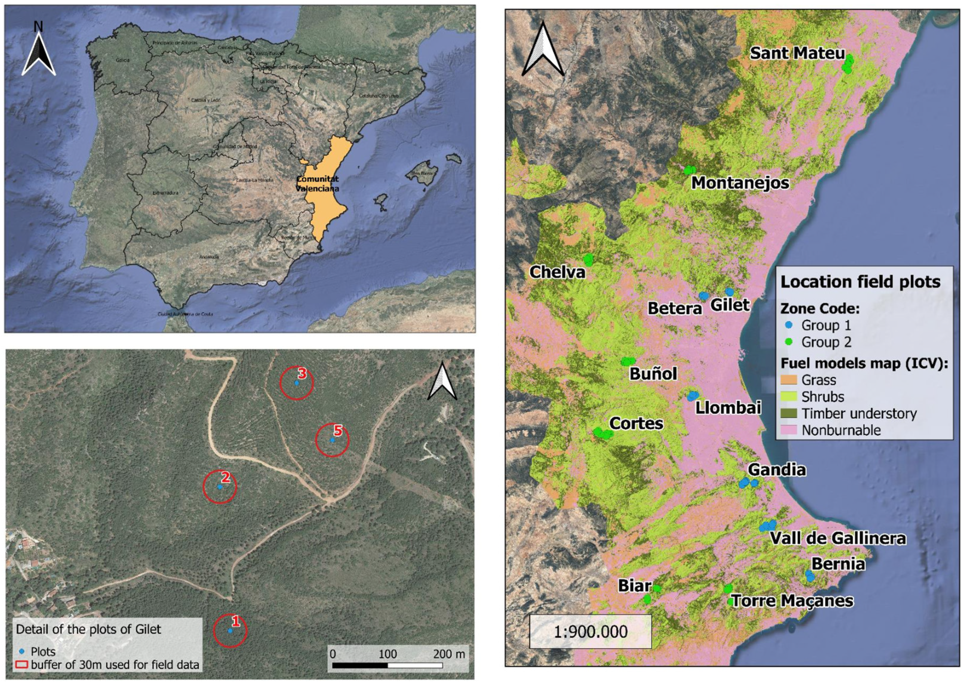
2.1. Study Area

The study plots are located in the Valencian region of Spain, in the east of the Iberian Peninsula (Figure 1) and with great influence from the Mediterranean Sea. The orography is highly variable throughout the entire territory, ranging from 0 to 1830 m of altitude above sea level, although most of the territory lies at altitudes below 1000 meters. In addition, the region presents a Mediterranean climate characterized by hot summers and mild winters, with low rainfall (350–550 mm per year). Rainfall frequently occurs in the fall and to a lesser extent in spring and winter. Summers are very dry and hot, causing long periods of drought and water deficits for the vegetation.

2.2. Field Data Collection

Small apical branches from various species of shrubs and trees were collected within 30-meter-radius plots containing a homogeneous vegetation type and structure, ensuring that the pixels corresponding to the satellite images represent the same or very similar areas to those collected in the field. Samples were collected every 15 days during the study period from June 2020 to November 2021. The samples were transported in sealed bags to prevent moisture loss, they were weighted wet, then oven-dried in the laboratory at 100 °C and weighed again to obtain the dry weight of each sample. LFMC corresponds to the water content of the vegetation calculated as the percentage of water contained in the species sampled in the field with respect to their dry weight, estimated with the following Formula (1):

LFMC = \frac{W f - W d}{W d} 100

(1)

where Wf corresponds to the fresh weight and Wd to the dry weight. The LFMC values per species and plot were added to a database throughout the study period. In addition, LFMC values per plot were calculated as a weighted average of LFMC values of the dominant species, considering the FCC (fraction of canopy cover) of each species as weights (see Table A1 in Appendix A). The percentiles of the weighted average values of LFMC in each plot were calculated. Then, the outliers found in the box and whisker plots were reviewed, to detect possible errors in the measurement of LFMC in any of the species.

This study is part of a research project where field data were collected in 88 specific plots of shrubs and trees, with the objective of developing a methodology for mapping the LFMC in the Valencian region of Spain with a spatial resolution of 10 m. In this particular study, field data in a subset of 50 plots were used to build the training sample, distributed throughout the Valencian region (see Figure 1 and Table A1). In the study area, there are differences in altitude, temperature, and rainfall, which are directly related to the natural vegetation present. Plot location was based on an even representation of different bioclimatic zones, as well as on the presence of dominant species of Mediterranean shrub. Many of the study plots were close enough to each other to estimate local variations (same zone code). These plots are part of a larger database, and they were selected according to the availability of field data, as well as on their location within the two main bioclimatic zones in our study area. The first column of Table A1 shows the numbering of the 50 plots in the database, and they were assigned to one of the two groups corresponding to the two bioclimatic zones (see Figure 1 and Table A2). There are variations in slope, aspect, and altitude within the two groups, even between plots within the same zone code (Table A1 and Table A2).

The thermo-Mediterranean group (group 1) corresponds to the area closer to the coast, with lower altitude; it is characterized by a climate with average annual air temperatures generally between 17 and 19 °C, ranging in the winter from mild to warm. The nature and distribution of the vegetation is mainly conditioned by the rainfall, as the chemical composition of the soil only seems to be decisive in certain areas with rainfall values above 400 mm. Precipitation affects the development of sclerophyllous forests composed of Pinus halepensis, Ulex parviflorus, Pistacia lentiscus, and Quercus coccifera.

The meso-Mediterranean group (group 2) contains the inland areas of the Valencian region with higher altitudes than the thermo-Mediterranean areas. Average annual air temperature ranges from 13 to 17 °C, and during the winter this interval is more pronounced. The distribution of the vegetation is conditioned by calcium carbonate-rich substratum soils and rainfall. Dense thickets of Pistacia lentiscus, trees such as Pinus pinaster, and repopulations of Pinus halepensis are very frequent.

2.3. Remote Sensing Data

Copernicus Sentinel-2 image bands were downloaded using the Google Earth Engine 14 environment, then spectral indices at 10 m spatial resolution were derived. The product used (Level 2A) is georeferenced and atmospherically corrected at bottom of atmosphere (BOA). Considering the different spatial resolutions of the image bands, we resampled to 10 m the bands with resolution of 20 m per pixel. Vegetation indices and water indices were considered, with formulas as described in Table 1.

The values of the indices NMDI, OSAVI, Vgreen, EVI, VARI, MSI, and TCARI were calculated for each plot on all sampling dates, considering an approximation of ±5 days between field data collection and the Sentinel-2 image acquisition date. Initially, a broader set of indices were considered, but those in Table 1 were the ones showing greater relationship with the LFMC data. In addition, the mean values of these spectral indices (period: June 2020–November 2021) were also calculated to obtain information about intersite vegetation differences. This is, the mean value of all dates considered was calculated for each index, in order to help characterize differences in greenness, photosynthetic activity of vegetation, and vegetation water content across sites. For example, Mean_EVI_10mS denotes the EVI average calculated in each plot using 10 m resolution Sentinel-2 data for all available dates within that period of time.

2.4. Meteorological Data

Daily mean surface air temperature and cumulative daily precipitation, collected from the Spanish Meteorological Agency (AEMET) at weather stations for the years 2020 and 2021, were used in this study. These values were interpolated in field plots using the Meteoland package [37]. The interpolation method used by Meteoland is similar to the inverse distance weighted (IDW) method but uses a truncated Gaussian filter for the selection of weather stations. The following variables were obtained: p60 (cumulative precipitation in the 60 days prior to field LFMC data acquisition) and t60 (average mean daily air temperatures in the 60 days prior to field LFMC data acquisition). Both are representative variables used in previous studies on live fuel moisture prediction [30].

The day of the year (DOY) was also considered, to describe seasonal variations of the LFMC. DOY was normalized to a range between [−π, π] and the sine (DOY_SIN) and cosine (DOY_COS) were calculated for use as predictors. These curves only vary in time, with values between −1 and 1, and describe the wettest or driest times of the year, respectively [38].

2.5. Statistical Analysis

The following methodological steps were used for the statistical analysis:

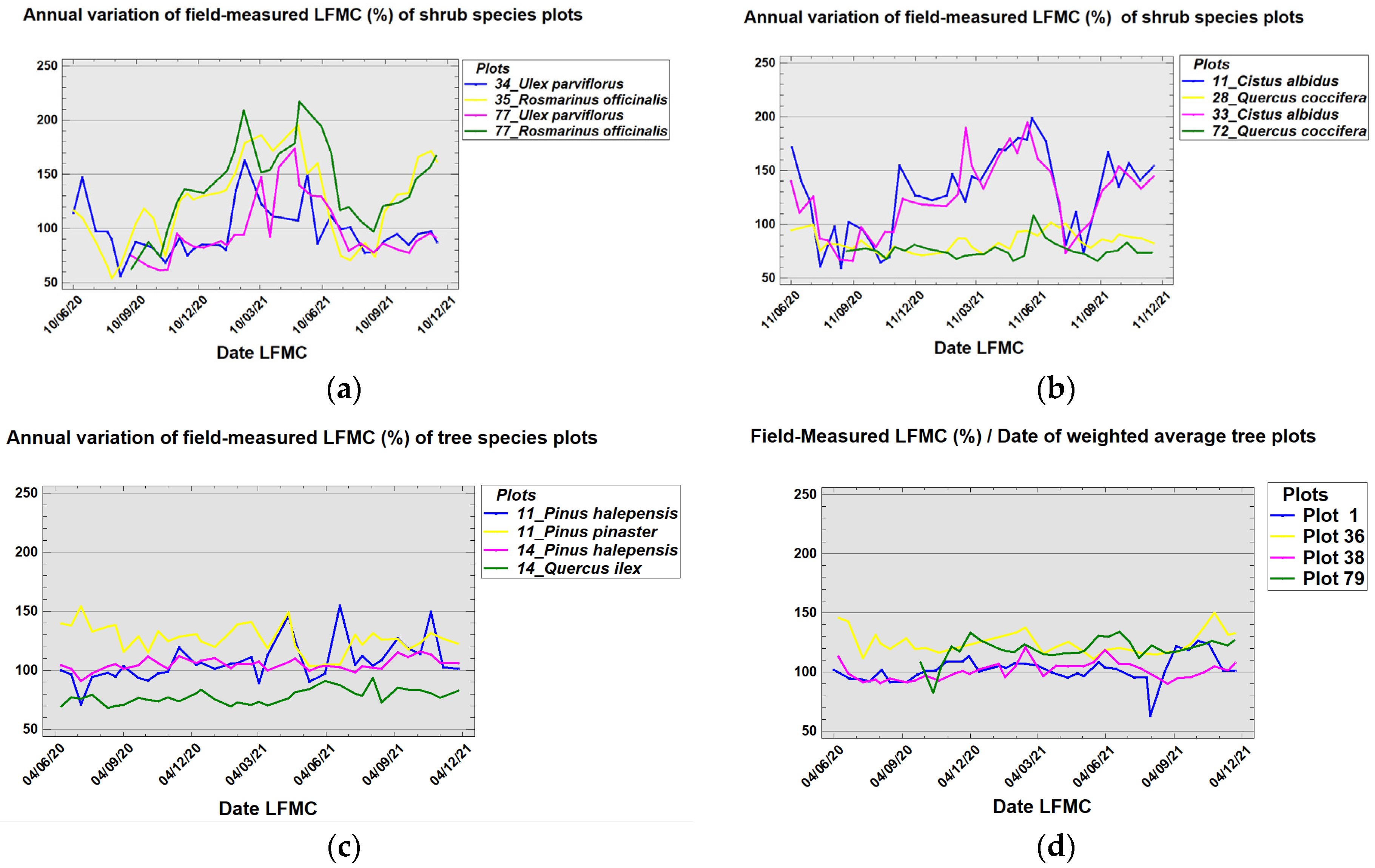
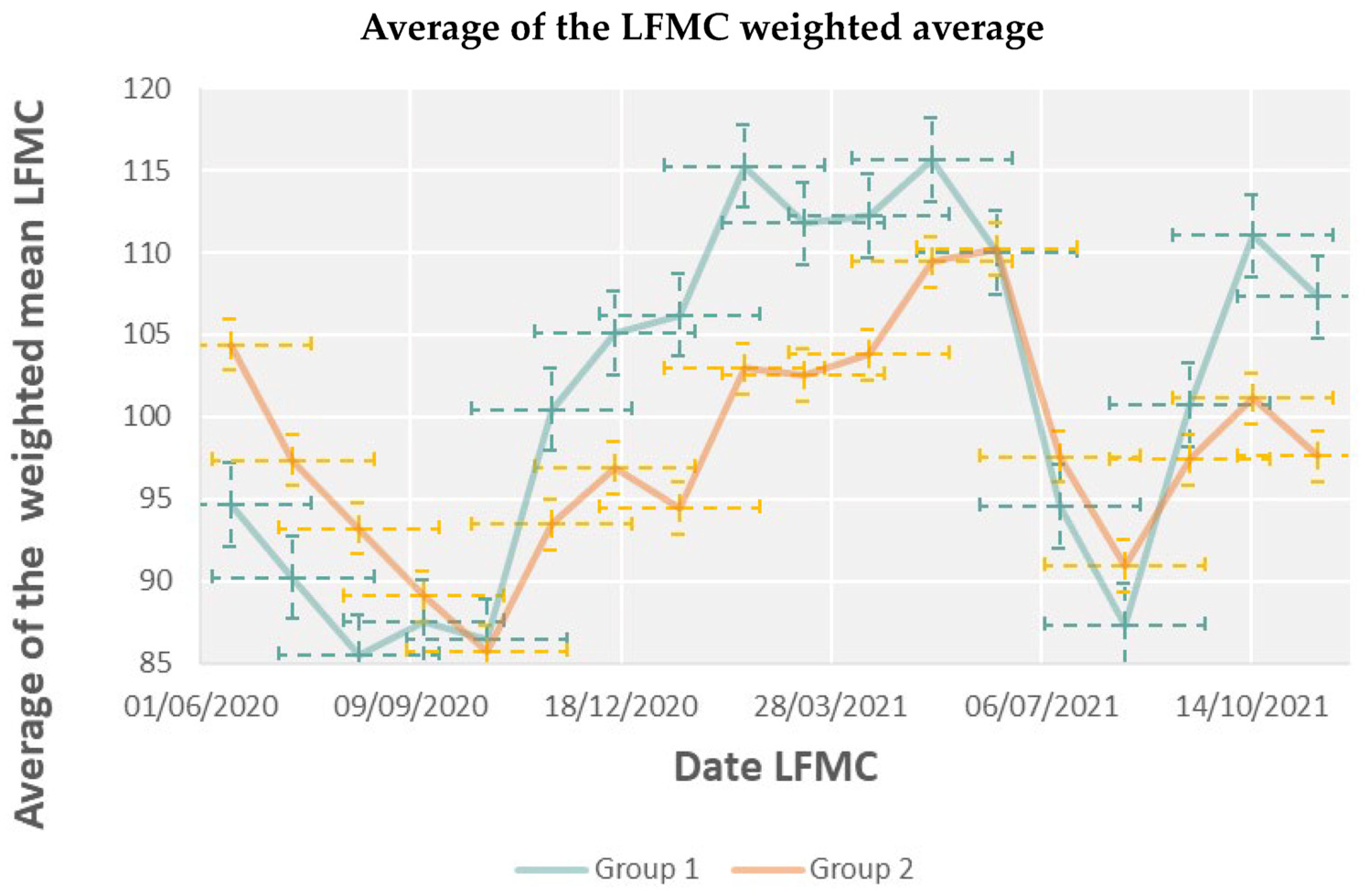
Analysis of the temporal variation of field LFMC data of several species in the period from June 2020 to November 2021 for the 50 sample plots distributed throughout the study area. Analysis of LFMC differences between shrub and tree strata and its influence on the weighted LFMC mean, using the fraction of canopy cover (FCC) of each species as weights;
Application of stepwise linear regression to compute the LFMC weighted average, considering the fuel models described in Table A1 and the groups of plots defined in Table A2. Moreover, a LFMC model for the Rosmarinus officinalis species was also calculated using LFMC data of that species in shrub plots where this was the dominant species. The spectral indices described in Table 1, together with time average of spectral indices in each plot, cumulative precipitation (p60), mean surface air temperature (t60), the sine and cosine of the DOY, slope, aspect, and altitude were used as predictor variables. The variance inflation factor (VIF) was calculated to analyze the collinearity of the variables. Predictor variables were revised when the VIF was greater than five, choosing only variables that were statistically significant with a VIF less than or equal to 5;
Application of generalized additive models with splines (GAMs). The data analyzed in this study were also fitted with generalized additive models (GAMs, “mgcv” R package), considering a gamma error distribution. In the designed models, spatial effects such as “2D smooth function (s(Xcoord,Ycoord)) of site locations” were added and a spatial term was also included, to lead to more precise estimates of the other model terms. According to this, site random effects (s(site, bs = “re”)) were considered. In this case, the zone code (“Zone Code”, Table A1) was used to identify the plot locations where LFMC samples were collected. On the other hand, for the time factor, the predictor for day of year (doy) was represented as a cyclic cubic spline (bs = “cc”), which allowed the models to explore the potential shape of the fitted trend more flexibly. For the analysis, in addition to the new spatial and temporal variables described, the same variables used in the linear regression were considered, since they had been previously selected based on a criterion of multicollinearity and correlation. However, for the final design of the model, only those significant variables within each group of plots studied were taken into account. In addition, the AIC (Akaike information criterion) value of all the candidates of each group was analyzed and compared, to determine the best model. This measure seeks to balance the goodness of fit of the model and its complexity, to avoid overfitting;
Evaluation of the linear regression and GAM models using the leave-one-out cross-validation method, analyzing the LFMC errors between observed and predicted results with these methodologies. Models were evaluated using adjusted R², RMSE (root mean square error), MAE (mean absolute error), and MBE (mean bias error) parameters [29]. Testing plots from other areas and dates were also used for additional evaluation;
Mapping LFMC estimates of a burnt area of the Valencian region using the designed model.

3. Results

3.1. Differences between Species in Field-Observed LFMC

Figure 2a shows the temporal evolution of the field-measured LFMC of two shrub species, Rosmarinus officinalis and Ulex parviflorus, in three different plots from the thermo-Mediterranean group. Plot numbers 34 and 35 are located less than a kilometer apart in the same zone code (Table A1). Rosmarinus officinalis usually shows higher values of LFMC than Ulex parviflorus, although the LFMC of both species presented a seasonal behavior. Figure 2b, represents the LFMC evolution for other shrub species, Cistus albidus and Quercus coccifera, in plots of the meso-Mediterranean group. In plots 11 and 33, Cistus albidus coexists with other shrub and tree species, while Quercus coccifera is one of the dominant species in plots 28 and 72. The measured LFMC of Cistus albidus was higher than that of Quercus coccifera, except for a few dates in the dry season. In addition, the LFMC of Cistus albidus showed seasonal variations, while the LFMC of Quercus coccifera presented a flatter series. In this way, in our study area, shrub species with different patterns of temporal variation of LFMC coexist with other species of trees. In addition, there is a spatial variation of LFMC in the same shrub species, even between plots of the same bioclimatic group. This demonstrates the need for an explicit spatial term in the GAM models (see Section 3.5).

Figure 2c represents the evolution of LFMC for the tree species Pinus halepensis, Pinus pinaster, and Quercus ilex in two different plots with the same zone code. The differences in LFMC values between these species are noticeable. The Quercus ilex LFMC values were the lowest in the entire time series, while the species Pinus Pinaster presented the highest values and Pinus halepensis had intermediate LFMC values, although with some differences between plots. In this way, the proportion of species present in each site marked the spatial differences in the values of the LFMC weighted average; in particular, this was noted in the plots with the highest presence of tree species. Figure 2d shows the evolution of the LFMC weighted average in several plots dominated by the tree stratum from the thermo-Mediterranean group, where two plots belong to the same zone code. Plots that contain the Pinus Pinaster species had a higher LFMC weighted average than plots where Pinus halepensis predominates or this species coexists with Quercus ilex. This can be interpreted as Pinus pinaster retaining more moisture. In addition, its LFMC behavior is more constant throughout the year.

Figure 3 shows the differences in the field-observed LFMC weighted average between shrubs plots from different bioclimatic zones. Plots of the thermo-Mediterranean group (Table A2) had slightly higher LFMC values during the winter and slightly lower during the summer, compared to the values of plots from the meso-Mediterranean group. These differences were partly due to the rainfall and average temperature regimes in each group area but also due to the dominant species present in each zone and their proportion of the FCC (fraction of canopy cover).

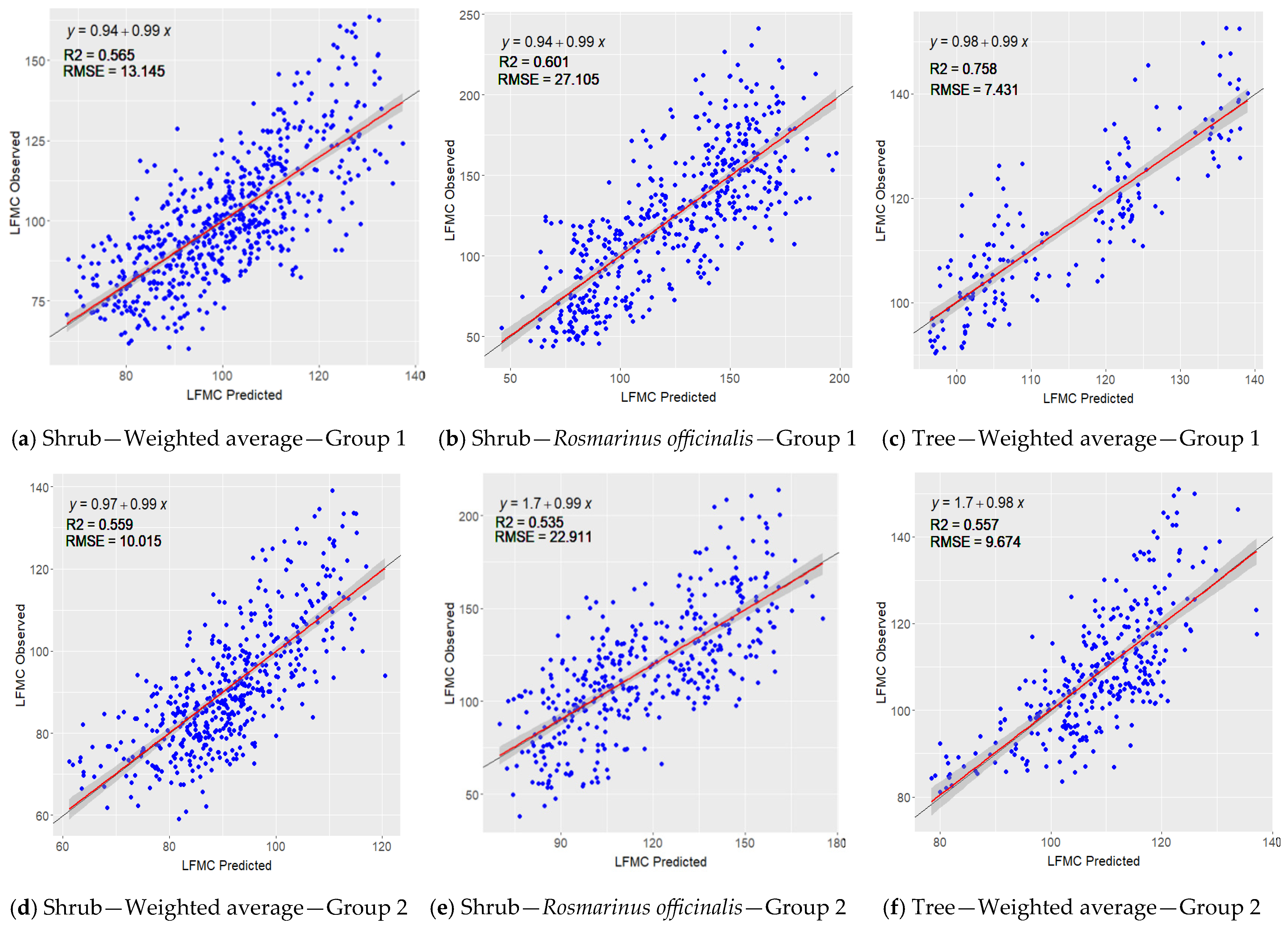
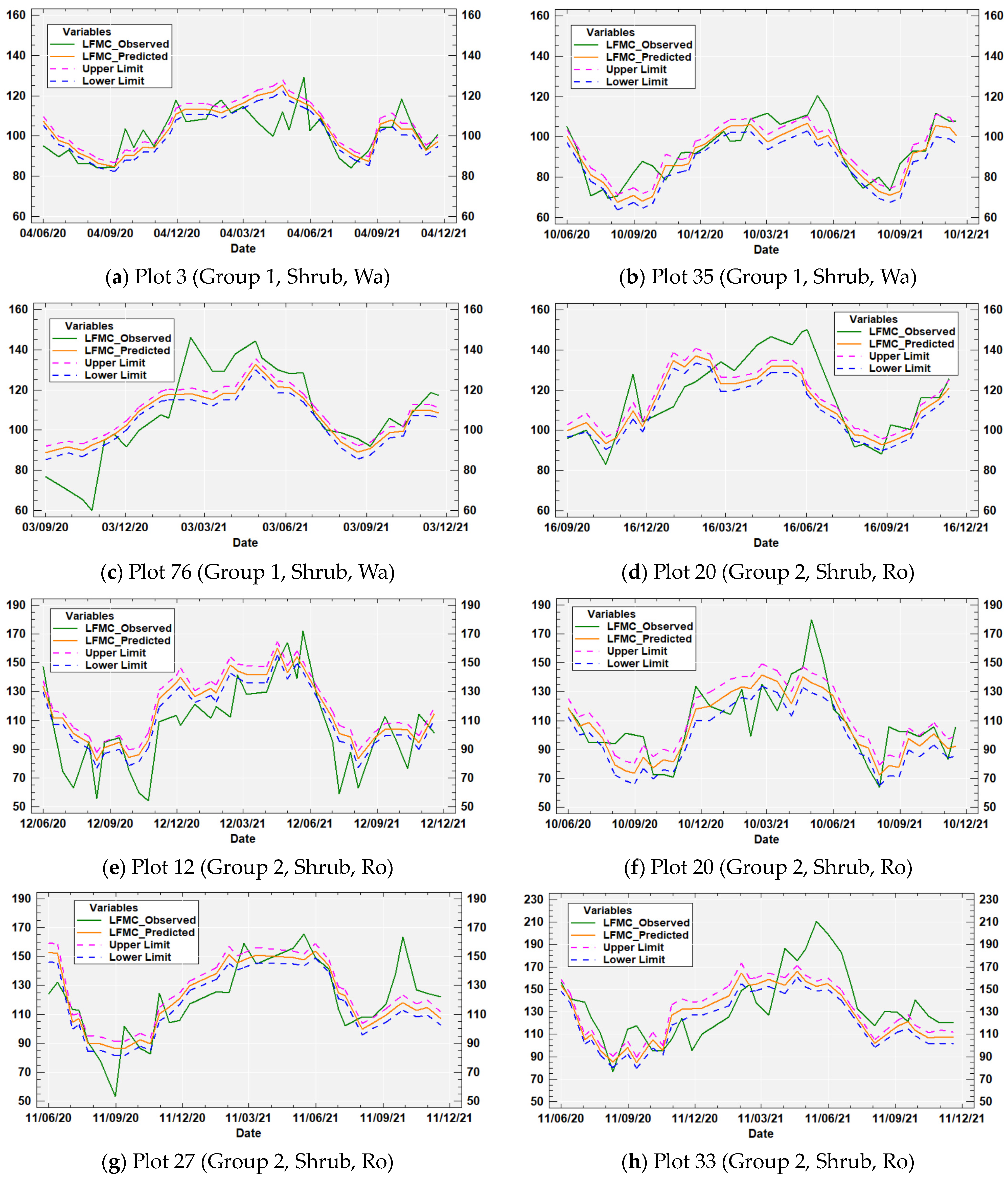
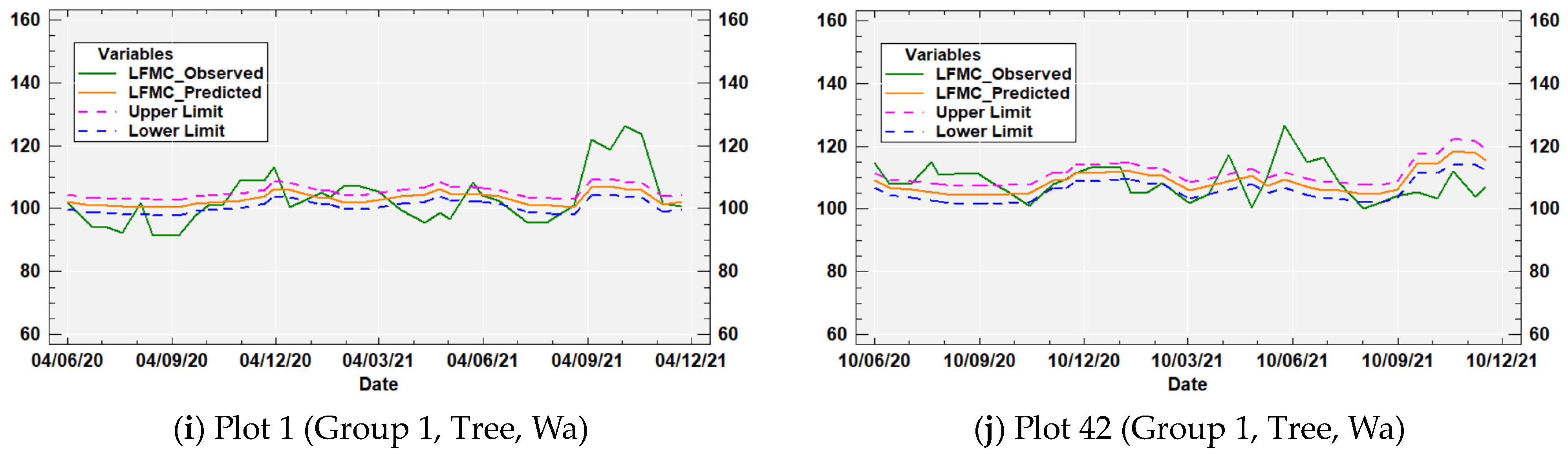
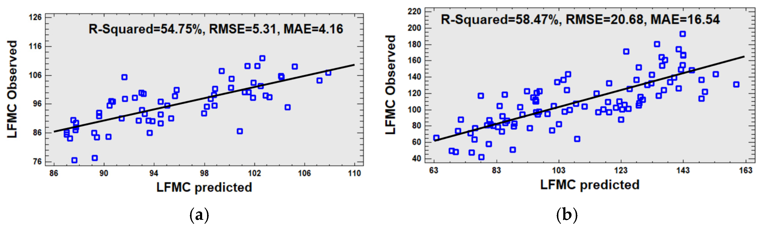
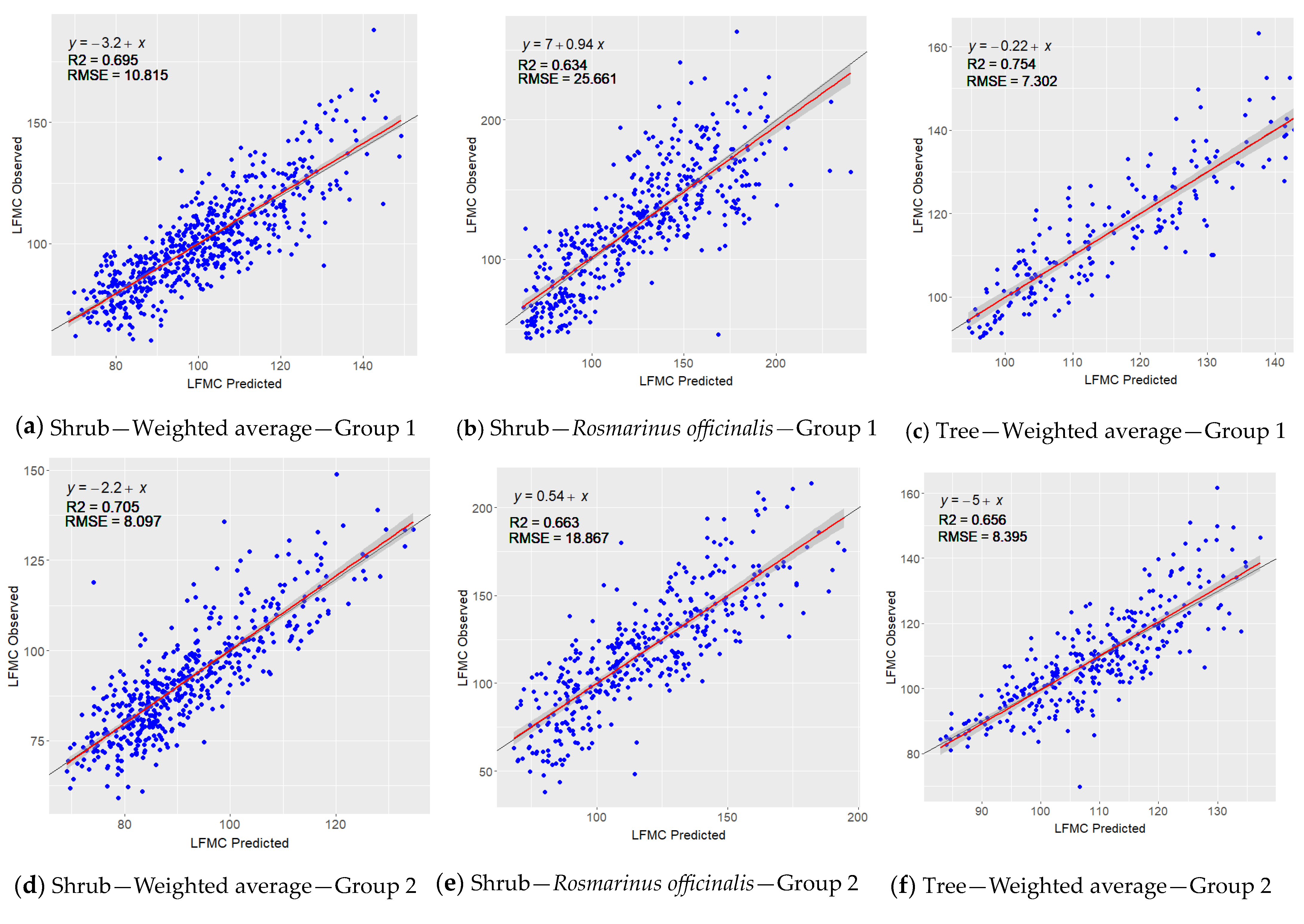
3.2. Models—LFMC Observed Values vs. LFMC Predicted Values

The models described in Table 2 were calculated using field-observed LFMC values from June 2020 to November 2021. Based on the bioclimatic groups of Table A2 in which the plots have been grouped, linear regression models were defined for the predictions of LFMC (LFMC weighted average and LFMC of Rosmarinus officinalis) in the fuel types considered in Table A1. Thus, three models were obtained for each plot group in Table A2: two in shrubs (one for the LFMC weighted average and another for LFMC of Rosmarinus officinalis species) and one in trees (LFMC weighted average). Table 2 shows the model coefficients by group, fuel type, and species considered to calculate the LFMC.

The number of explanatory variables used in the models in Table 2 varied between 4 and 6, highlighting NMDI, p60, and DOY_SIN as the most important. However, the spectral index used in the model depended on the fuel type and the LFMC prediction being considered (weighted average of all species or only Rosmarinus officinalis species). Information of spatial differences between plots was obtained using the average of each spectral index per plot for all available dates, or through topographic factors, such as elevation or slope. All predictors were statistically significant at a 95% confidence level, and the VIF (variance inflation factor) was less than 5 for all of them, which is indicative of non-multicollinearity.

Figure 4 shows comparative graphs of the LFMC predictions and field-observed LFMC values for the different study groups. The black line represents slope 1 and the origin at 0, while the red line represents the regression line. The equations obtained for each case are described in the graphs. In all the models, the slope is very close to 1, while the intercept is close to zero. The coincidence of the linear regression line and the line representing slope 1 indicates that there was no significant bias in the model. However, in some plots, there seems to be a slight increase of the variance in the observed LFMC values as the mean increases.

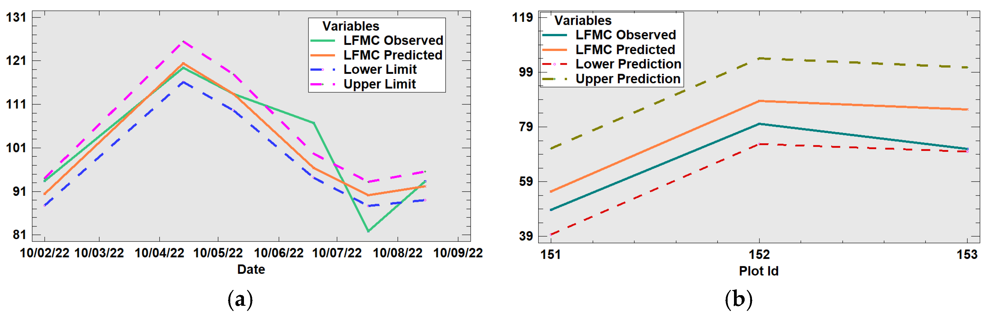
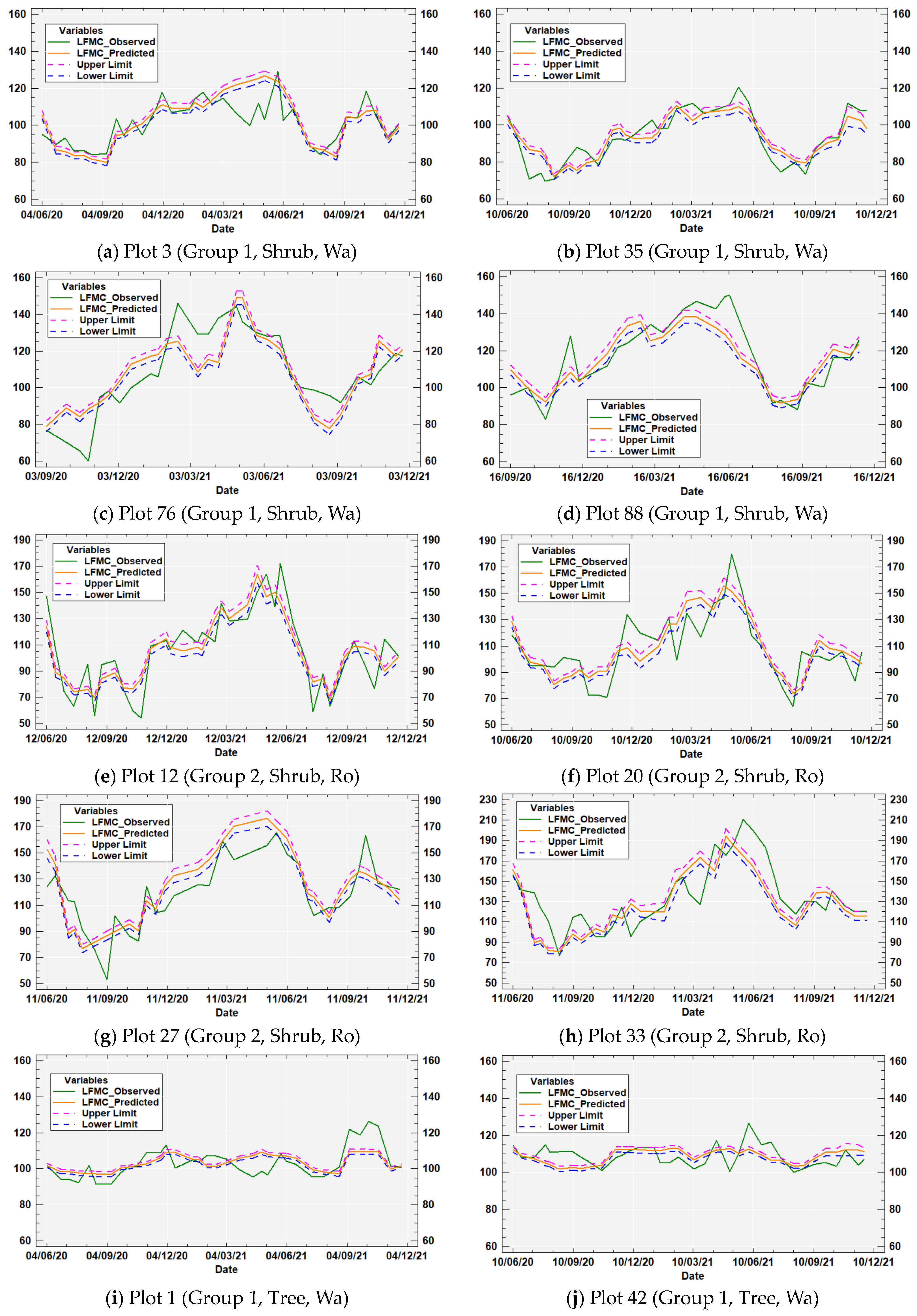
3.3. Cross-Validation and Extrapolation to Other Plots and Dates

Multiple linear regression and GAMs models were validated using the leave-one-out cross validation method. The graphs and results obtained for the GAMs are explained in Section 3.5. Therefore, this section specifically refers to the models designed using linear regression.

The adjusted R² values of the models ranged from 52.1% to 74.4% (Table 2). The highest percentage was presented by the model of Group 1 in the prediction of LFMC weighted average where tree species were dominant. Regarding the error metrics, the RMSE values were between 7.4 and 27.7 and MAE varied between 5.9 and 23.0. The highest values of RMSE and MAE were obtained in the prediction of the LFMC of Rosmarinus officinalis, which is one of the shrub species with the greatest variability. In addition, MBE varied between −0.021 and 0.006, which reflects a good fit.

Figure 5 shows the temporal evolution of the field-observed LFMC values and LFMC predicted values in several plots using the models described in Table 2. Different LFMC behaviors were observed according to fuel types (shrub or tree) and type of LFMC prediction (Rosmarinus officinalis or weighted average of all species). Shrub species showed clear seasonal variations (Figure 5a–h) compared to tree species, whose LFMC behavior was flatter, with almost no seasonal variability (Figure 5i,j). However, in both cases the models may be able to describe the changes that occur between plots at the spatial level. The proportion of species existing in each plot influenced the value of the LFMC weighted average and our models could reproduce the changes observed between plots of the same group. The lower temporal variation of LFMC in the tree plots led to lower values of RMSE and MAE.

In the shrub plots of Figure 5a–h, we can observe how the proposed models reproduced a sharp decrease in LFMC values during the months of June, July, August, and September (dry season). Notice that, depending on the species considered, the LFMC range values in the Y-axis scale changes. The LFMC values of Rosmarinus officinalis were greater than those of the weighted average (obtained by considering all the species present in the plots and their fraction of canopy cover).

On the other hand, in order to provide more robust evidence of predictive power of the linear regression models described in Table 2, an independent validation using data from different geographical locations in the same time period was performed. Figure 6 shows the results obtained in some plots located in areas classified in the shrub fuel model type. Plot id numbers 15 and 18 are in the thermo-Mediterranean zone and their predicted LFMC weighted average was calculated using the first model described in Table 2. The R² between the predicted and observed LFMC in these plots was similar to the R² adjusted of this model, while the RMSE and MAE values were slightly lower. The LFMC predictions of the Rosmarinus officinalis species reached values greater than the LFMC weighted averages, and since most of the errors occurred at extreme values then RMSE and MAE values were higher (Figure 6b). In any case, the values obtained for these statistics are similar to those shown in Table 2 for the model used in the predictions (G = 2, Ft = Sh, Sp = Ro).

Moreover, an alternative evaluation was carried out with additional independent samples in other time periods outside the range of dates used to calibrate the models. Thus, the LFMC measurements not used to train the models were collected in additional plots during the year 2022, in order to evaluate the temporal extrapolation of the models. Figure 7a shows a comparison between the field-observed and predicted LFMC weighted averages in one of the plots located in a shrub area in the Chelva zone code. The errors for various dates in 2022 were within the 95% confidence limits for the mean response. In addition, LFMCs of Rosmarinus officinalis species were measured in three plots during a wildfire near Bejís municipality in August 2022. Figure 7b compares these values observed in the field with those predicted on a date prior to the fire. The predicted LFMC values were higher than those observed, but it should be noticed that the latter were collected a few days later. Despite this, the LFMCs observed in field were within the 95% prediction limits for new observations.

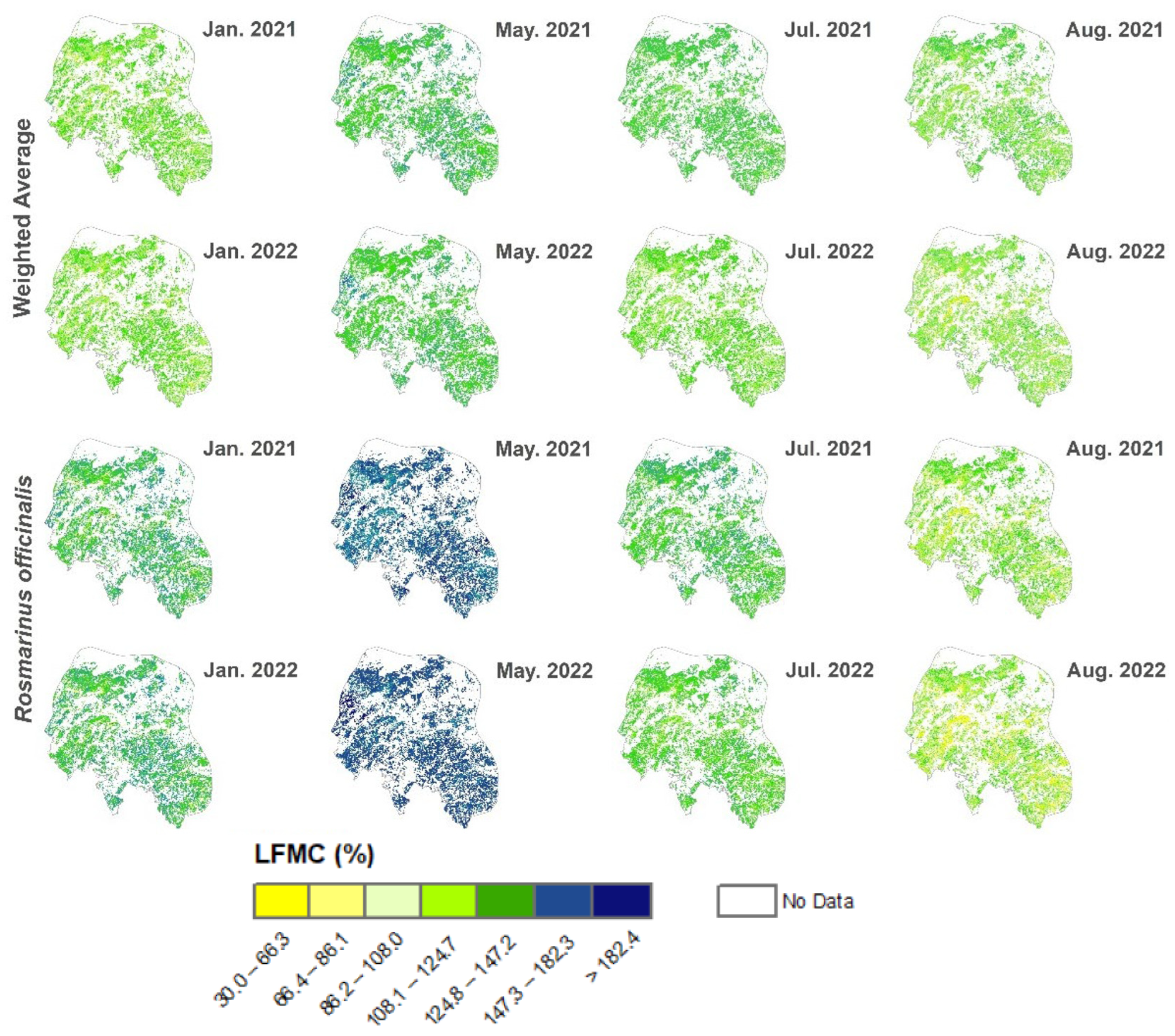
3.4. Prediction Maps

The models described in Table 2 were used to obtain LFMC prediction maps in an area where a forest fire occurred in August 2022 (Figure 8), around the municipality of Bejís, located in an inland zone of our study area, south of Montanejos zone and north of Chelva (see Figure 1). For the elaboration of the maps, we used the model corresponding to the meso-Mediterranean bioclimatic zone.

The LFMC predicted values obtained with the weighted average model were low in January 2021, although they later increased for May 2021, after the rainy season. They decreased during the dry season, reaching very low values (LFMC weighted average <66) in August 2021. A similar behavior was observed for 2022. The lowest values (yellow color) were observed in August 2022, showing the dry condition of the vegetation prior to the forest fire that started on 15 August 2022. The LFMC predictions obtained with Rosmarinus officinalis model showed higher range of variation (Figure 8). Their values were high (LFMC > 200) in May 2021, which reflects very humid vegetation, while in July 2021 low LFMC values were observed, corresponding to a dry situation that became extremely dry in August. Similar behavior was observed in 2022.

3.5. GAM (Generalized Additive Models)

When applying the GAMs, a notable improvement was obtained in the fit of the data, except in the cases of tree zones in Groups 1 and 2. In these cases, the difference with respect to the linear model was almost imperceptible (0.3%–0.8%, R²). Table 3 shows the coefficients of the models by group, fuel type, and species considered to calculate the LFMC, along with the corresponding results and error metrics. The adjusted R² values of the models ranged from 53.4% to 74.1% (Table 3). The highest percentage was presented by the model of Group 1 in the prediction of LFMC weighted average where tree species were dominant. Regarding the error metrics, the RMSE values ranged from 7.6 to 24.8, and MAE from 5.9 to 19.6. The highest values of RMSE and MAE were obtained in the prediction of the LFMC of Rosmarinus officinalis, as in the case of the linear models. Finally, the MBE varied between −0.081 and 0.023.

As shown in Table 3, the variable DOY_SIN (used in the linear analysis) was only considered in the model of one of the groups: (G1—Shrub—Weighted average) based on the analysis of the AIC criteria. In all other cases, the values of this parameter (AIC) were lower when using the variable “doy” than when using the sine and cosine transformations. “G1-Tree-Weighted average” was the only group that did not use the “doy” parameter, as it was not significant. On the other hand, Table 3 shows that the “Zone_code” variable, despite the fact that it was considered in the analysis of all six groups, was discarded in four groups and accepted in two groups, with these corresponding to the “G2—Shrub—Rosmarinus officinalis” and the “G2—Tree—Weighted average”.

According to this GAM analysis, Figure 9 shows comparative graphs of the LFMC predictions and field-observed LFMC values for the different study groups. The black line represents slope 1 and the origin at 0, while the red line represents the regression line. The equations obtained for each case are described in the graphs and reflect the good fit provided by this type of model.

Additionally, predictions for each plot—analyzed with the previous method—from fitted GAMs were generated, and they are shown in Figure 10, along with their respective bounds (upper and lower).

4. Discussion

Different species coexist in the plots of our study area in different proportions. There are certain species that are prone to large fluctuations in LFMC, which, upon changes of atmospheric conditions, tend to gain and lose water more easily and faster than others. Thanks to the modification of their leaves, stems, and roots, they are able to absorb or retain water for long periods of time, in order to survive extreme climate conditions. Xerophytic plants have long roots and usually very small leaves, which prevent unnecessary water loss. For example, Rosmarinus officinalis, Cistus albidus, and Quercus coccifera are xerophytic species adapted to drought conditions, each of them in a different way. Ulex parviflorus is a species that dries out very quickly and does not retain as much moisture, which makes it very dangerous in terms of fire spread. Some xerophytic plants are pyrophilous, adapted to suffer from fires, and they are common in our study area. On the other hand, tree species of the Mediterranean forest are adapted to drought, and their moisture tends to be constant throughout the year. Quercus ilex has hard toothed leaves, which retain moisture. Pinus pinaster and Pinus halepensis are characterized by their needle-shaped leaves, which absorb moisture and lose very little water. Thus, the sampled species in each plot (Table A1) were averaged to represent the LFMC for the same date and location, using the FCC information for each species. In this way, the composition of species at each site directly influenced the value of LFMC considered to train our models. Such an LFMC weighted average can be used as a measure of potential fire risk. However, in our study region, it was also interesting to calculate LFMC values in individual common species that dry out quickly, such as Rosmarinus officinalis, which are found in a high number of plots with an FCC greater than 10. Since this is one of the most representative xerophytic species in our study area, the LFMC for Rosmarinus officinalis was also predicted in shrub areas. There were 26 plots with Rosmarinus officinalis representing an FCC greater than 10%. Ulex parviflorus and Rosmarinus officinalis coincided in 21 plots. However, there were only 7 plots where Ulex parviflorus represented an FCC greater than 10%.

A model calculated for the LFMC weighted average in tree zones had the highest adjusted R² (74.39%). This must have been due to the fact that the spatial variability was much greater than the temporal variability in these tree areas, as we mentioned before when analyzing the LFMC changes in the tree species. Therefore, three of the four predictors considered in this model only changed at the spatial level (slope, mean of MSI, and mean of TCARI). This also implies that smaller values of RMSE and MAE were obtained in the models for tree areas. On the other hand, the highest errors between the observed and mean predicted values occurred in the estimation of the LFMC of Rosmarinus officinalis species, in which the temporal variability was much greater, with LFMC values above 200 in the humid season, but below 60 in the dry season. Table A5 in Appendix A shows the proportion of observations that were within the 50% bounds on the predictions, using size 20 LFMC intervals. There was a greater proportion of data at the extreme intervals of LFMCs that were outside these prediction limits, but in the case of the prediction of LFMC of the species Rosmarinus officinalis, there were many more values measured in the field below 60 and above 140.

We explored the effect of introducing a categorical variable into the models, considering mixed models that take into account the zone code with random effects. The RMSE and MAE values obtained in the estimation models of the LFMC of Rosmarinus officinalis species with these mixed models (see Table A4 in Appendix A) were slightly lower than those obtained in Table 2 with linear models, while the adjusted R² increased. However, these mixed models are more difficult to apply for generating cartography in areas that do not have data to calibrate the models, such as the one used in Figure 8. We tested the inclusion of the latitude and longitude variables in the linear models. In the case of the linear models that predicted the LFMC weighted average, our methodology discarded both spatial coordinates, as they were not significant. However, in the LFMC estimation of the Rosmarinus officinalis species, latitude could be introduced in the thermo-Mediterranean group (group 1), whereas longitude could be selected in the meso-Mediterranean group (group 2). Thus, spatial effects were considered for inclusion in the generalized additive models with splines via a 2D smooth function of site locations, together with a term with site random effects.

In this paper, empirical models were developed using spectral indices from Sentinel-2 images and meteorological data (cumulative precipitation and averaged surface air temperature). Additional topographic and static seasonal variables were also considered and tested. Six models were fitted to estimate the LFMC weighted average, and the LFMC of the Rosmarinus officinalis species, attending to two vegetation types and two bioclimatic zones, which showed the great potential of using empirical models with remote sensing data, together with topographic and meteorological data, to spatially monitor the LFMC of shrub and tree species at a spatial resolution of 10 m. Moreover, a seasonal trend was considered using the functions DOY_SIN or DOY_COS, which are defined as the sine and cosine of the day of the year. These predictors had a significant influence on the LFMC estimates, especially on the shrub models, due to the seasonal variation in LFMC. Cunill-Camprubí et al. [27] commented that DOY_SIN reflects the average annual pattern in soil water availability, while DOY_COS is more related to changes in the surface air temperature. The sine and cosine of the day of the year are useful variables to reflect typical seasonal trends, but they do not provide real information about a date, so all models described in this paper included a cumulative precipitation variable (p60) to extrapolate to years with different meteorological conditions. Moreover DOY_COS was used in combination with a mean surface air temperature variable (t60).

NMDI was the spectral index with the highest correlation with LFMC in shrub areas within the period from June 2020 to November 2021. NMDI is related to the humidity of the vegetation, and it is highly linearly related to the NDMI index, which was used in [30] to predict LFMC averages and to obtain a model in shrub areas, but only in the dry season. Moreover, the model described in [30] was obtained in a smaller yet similar study area. In our work, the stepwise process we followed to select variables did not include the NDMI in the models. However, other spectral indices related to vegetation and water content (EVI, OSAVI, and Vgreen) were used to estimate the weighted mean of LFMC in shrub zones or wooded areas, as well as of Rosmarinus officinalis species in shrub plots. Likewise, the means of spectral indices were used (Mean_EVI, Mean_VARI, Mean_MSI, and Mean_TCARI), improving the performance of the model, as in [39]. These averages took a constant value in each plot and allowed modifying the intercept in each site considering its spectral characteristics. Along with these variables, morphological variables (slope, altitude) were added, further improving the performance of the model. In the case of shrub plots, the means of vegetation indices together with the altitude appeared as predictors in the models of the thermo-Mediterranean group. In contrast, in the meso-Mediterranean group, the slope intervened to modify the constant of the model but only at the spatial level.

Among the meteorological variables, the cumulative rainfall in the previous 60 days (p60) was part of all the models obtained for the estimation of LFMC. Other time periods (7, 15, and 30 previous days) were also tested, but p60 was always the precipitation variable with the highest correlation with LFMC and the one chosen using the stepwise regression method. Precipitation provides relevant information for the models at a temporal and spatial level. The interpolation process used to estimate precipitation also marks the differences in plots very close to each other. Spectral variables were also able to represent the LFMC changes, both at the spatial and temporal levels, even in plots located in nearby areas. In order to obtain a good fit, it seems to be convenient to use both types of information: spectral and meteorological [20,23,24]. The average air temperatures in the previous 7, 15, 30, and 60 days were also considered, and the latter (t60) was selected in a shrub model, completing the seasonal information introduced through the cosine of the day of the year. Variable t60 also varies spatially; in our case, point values were interpolated from surface air temperature data obtained from a set of surrounding weather stations.

Different models were built in two bioclimatic strata for the prediction of LFMC in grouped plot locations. The evaluation of the models for the study groups presented sound results in each of the locations analyzed, since the predicted values were mostly within the range of the field data for the complete study period (June 2020–November 2021). The extrapolation of these models for mapping LFMC in other subsequent time periods was also tested, analyzing the LFMC maps obtained in an area where a major forest fire occurred in 2022. Historically, the largest average monthly burned area and the highest number of fires in the period 2002–2019 in our study area occurred from June to October (see: https://gwis.jrc.ec.europa.eu/apps/country.profile/charts, last accessed 30 November 2022), which coincides with the dry season. One of the main benefits of covering all seasons of the year is being able to predict LFMC values for any date, which is important in fire risk monitoring and fire prevention planning, especially considering the scenario of our study area.

Regarding previous studies using Sentinel-2 data, our results are similar to those obtained in [25,40]. However, the models in [25] were only applied to a monospecific shrubland site, and the models in [40] used time series acquired from active (Sentinel-1) and passive (Sentinel-2) sensors. In [25], it is stated that Sentinel-2 may be a good alternative to MODIS if daily estimations are not a priority but where higher spatial resolution is needed (e.g., patchy vegetation areas). To build our models, we used 50 plots, some of which were less than 1 km apart, aiming to obtain maps with a high spatial resolution (10 m). Accurate results were obtained when extrapolating the models to estimate LFMC in the dry season of the next year from the one used for training. Despite this, it is important to consider an annual model calibration phase (prior to use) for predicting LFMC values more accurately at different sites and in different years, due to the changes in climatic conditions, particularly in evidence in recent years.

This study has some limitations that must be considered when interpreting its results. First, it is important to note that the study was carried out in a specific geographical region and ecosystem, meaning that the results may not be applicable to other areas with different climatic and ecological conditions. Second, the study focused on a limited number of species and fuel types (trees (24%) and shrubs (46%)), which may not reflect the full diversity of vegetation present in the area. However, the moisture content of the most characteristic and representative species of the Mediterranean forest, and which are the most influential in the spread of forest fires, were sampled. In each plot and date, only from one to three LFMC samples of each species were taken, due to logistic limitations on drying the samples. Thus, we were not able to study possible variations between individuals of the same species in the same plot. Fourth, the introduction of variables defined from other environmental factors, such as the speed of the maximum gusts of wind or the relative humidity, may have slightly increased the precision of the models, as this was verified in the preliminary study described in [30]. However, many meteorological stations with precipitation and temperature data do not have data on these variables, increasing the errors in the interpolation of such meteorological data. For this reason, in this work, only meteorological data of cumulative precipitation and surface air temperature were considered. In addition, the study only covered a period of 1.5 years, which may not be sufficient to capture long-term trends in moisture content variability and establish robust models. Finally, the study did not consider the effects of anthropogenic factors such as land use change and fire suppression on the LFMC, because we used fuel model mapping with a publication date of 23 February 2021, which could have influenced the accuracy of the models. It is important to take into account these potential limitations and deficiencies when mapping other areas of our study region and in other periods of time.

5. Conclusions

In this study, an analysis of the combination of Sentinel-2, topographic, and meteorological data to predict LFMC with a spatial resolution of 10 meters was carried out in a Mediterranean ecosystem with different types of vegetation coexisting. Empirical models for estimating LFMC were obtained using stepwise linear regression and generalized additive models with splines (GAMs), using data obtained during the period June 2020–November 2021, in 50 plots organized into 2 groups, and defined based on bioclimatic zones. Two LFMC models were differentiated: those for shrub species and those for tree dominant plots. Models were calculated considering the weighted average of LFMC values for the dominant species of shrubs or trees. Since Rosmarinus officinalis is one of the most representative species in the area, LFMC models considering only this species were also obtained in the shrub plots.

The number of independent variables used in models was between 4 and 6; among these, the cumulative rainfall in the previous 60 days (p60) was part of all the models. The results obtained showed that the spectral indices, especially the NMDI, were sensitive to LFMC changes at a temporal and spatial level. The topographic variables (slope and altitude) and the means of various spectral indices (static variables) also played a very important role in models, since they marked spatial differences and contributed to the reduction of model errors.

This study is an extension of that described in [30] over a longer study period, including the dry and humid seasons, considering a broader set of sampling points in shrub areas but also applied to areas with tree dominant species. The proposed models were adapted to the seasonal changes of LFMC, and maps were created to visualize the LFMC spatial evolution several months before the occurrence of a major wildfire. Although GAMs models are capable of predicting LFMC with greater precision, models obtained with multiple linear regression may also be adequate for mapping LFMC with a 10 m resolution using Sentinel-2 images, due to their easy implementation and speed of calculation.

Author Contributions

Conceptualization, M.A.A., R.E.-B., Á.B.-B. and L.Á.R.; methodology, M.A.A., R.E.-B., Á.B.-B. and L.Á.R.; software, M.A.A., R.E.-B. and Á.B.-B.; validation, M.A.A. and Á.B.-B.; formal analysis, M.A.A., R.E.-B., Á.B.-B. and L.Á.R.; investigation, M.A.A., R.E.-B., Á.B.-B. and L.Á.R.; resources, M.A.A., R.E.-B. and Á.B.-B.; data curation, M.A.A., R.E.-B. and Á.B.-B.; writing—original draft preparation, M.A.A., R.E.-B., Á.B.-B. and L.Á.R.; writing—review and editing, M.A.A., R.E.-B., Á.B.-B. and L.Á.R.; visualization, M.A.A., R.E.-B., Á.B.-B. and L.Á.R.; supervision, M.A.A., R.E.-B., Á.B.-B. and L.Á.R.; project administration, M.A.A. and Á.B.-B.; funding acquisition, Á.B.-B. and L.Á.R. All authors have read and agreed to the published version of the manuscript.

Funding

M^a Alicia Arcos gives thanks for the help received by the Universitat Politècnica de València through a pre-doctoral contract financed in the call, PAID-01-19, subprogram 1. This research was funded by through a collaboration agreement between the company Red Eléctrica de España S.A.U. and the Universitat Politècnica de València (2020–2023), as well as the research project PID2020-117808RB-C21 funded by MCIN/AEI/10.13039/501100011033 and by ESF Investing in your future.

Data Availability Statement

Sentinel-2 data are freely available. The in situ LFMC and meteorological data were obtained from the Valencian regional government under a specific research agreement.

Acknowledgments

The authors thank the Public Company VAERSA and the Direcció General de Prevenció d’Incendis Forestals of the Generalitat Valenciana for providing the LFMC measurement data in the field and the meteorological data through the AEMET.

Conflicts of Interest

The authors declare no conflict of interest.

Appendix A

Table A1. Study plots of the Valencian region, sampled species with their FCC (fraction of canopy cover) and fuel types (T (tree); Sh (shrub)) based on Scott and Burgan models (source: http://agroambient.gva.es/es/web/prevencion-de-incendios/models-de-combustible, accessed 16 December 2022).

Plot id	Zone Code	Slope (°)	Aspect (°)	Altitude (m)	Species (% FCC)	Fuel Types
1	Gilet	26.47	0.24	267.56	Pinus halepensis (99), Juniperus oxycedrus (7), Pistacia lentiscus (10), Quercus coccifera (10), Erica multiflora (7), Ulex parviflorus (3),	T
2	Gilet	25.19	166.35	254.76	Pinus halepensis (35), Rosmarinus officinalis (25), Quercus coccifera (20), Erica multiflora (20), Pistacia lentiscus (20),	Sh
3	Gilet	16.23	229.44	309.87	Pinus halepensis (70), Rosmarinus officinalis (40), Pistacia lentiscus (30), Phillyrea angustifolia (20), Erica multiflora (3),	Sh
5	Gilet	25.87	109.90	295.04	Pinus halepensis (20), Rosmarinus officinalis (30), Quercus coccifera (10), Phillyrea angustifolia (12), Pistacia lentiscus (17),	Sh
6	Bétera	7.79	162.32	212.29	Pinus halepensis (20), Juniperus oxycedrus (10), Rosmarinus officinalis (30), Pistacia lentiscus (7),	Sh
7	Bétera	3.67	115.97	201.77	Pinus halepensis (40), Juniperus oxycedrus (20), Rosmarinus officinalis (35), Quercus coccifera (5), Pistacia lentiscus (3), Stipa tenacissima (30),	Sh
9	Bétera	7.25	232.11	182.60	Pinus halepensis (75), Rosmarinus officinalis (25), Quercus coccifera (10), Juniperus oxycedrus (15), Pistacia lentiscus (30),	Sh
11	Chelva	2.56	301.57	976.01	Pinus halepensis (35), Pinus pinaster (35), Cistus albidus (10), Juniperus oxycedrus (30), Juniperus phoenicea (25),	T
12	Chelva	4.67	190.52	751.25	Pinus halepensis (20), Rosmarinus officinalis (10), Arbutus unedo (20), Juniperus oxycedrus (30), Erica multiflora (15), Ulex parviflorus (10),	Sh
13	Chelva	12.83	351.48	950.85	Pinus halepensis (10), Quercus ilex (35), Rosmarinus officinalis (15), Quercus coccifera (40), Juniperus oxycedrus (15), Juniperus phoenicea (10),	Sh
17	Llombai	16.57	291.88	233.48	Pinus halepensis (7), Rosmarinus officinalis (30), Quercus coccifera (45), Juniperus oxycedrus (5), Erica multiflora (15),	Sh
19	Llombai	12.71	57.57	265.09	Pinus halepensis (15), Rosmarinus officinalis (25), Quercus coccifera (35), Erica multiflora (20),	Sh
20	Buñol	24.42	103.56	547.70	Pinus halepensis (20), Rosmarinus officinalis (30), Ulex parviflorus (10), Juniperus oxycedrus (15), Quercus coccifera (5), Erica multiflora (30),	Sh
21	Buñol	8.74	226.00	679.45	Rosmarinus officinalis (50), Quercus coccifera (50), Ulex parviflorus (5), Juniperus oxycedrus (20), Erica multiflora (7),	Sh
24	Buñol	14.26	338.90	678.31	Pinus halepensis (10), Rosmarinus officinalis (30), Quercus coccifera (50), Juniperus oxycedrus (30), Erica multiflora (7),	Sh
26	Cortes	2.27	23.90	878.46	Pinus halepensis (15), Pinus pinaster (25), Quercus ilex (4), Rosmarinus officinalis (30), Quercus coccifera (3), Juniperus oxycedrus (15), Ulex parviflorus (3), Cistus albidus (3),	Sh
27	Cortes	3.94	0.73	888.48	Pinus halepensis (5), Quercus ilex (10), Rosmarinus officinalis (20), Quercus coccifera (20), Juniperus oxycedrus (10), Cistus albidus (3),	Sh
28	Cortes	11.36	107.12	889.76	Quercus ilex (15), Rosmarinus officinalis (10), Quercus coccifera (30), Juniperus oxycedrus (10), Cistus albidus (3),	Sh
29	Cortes	1.34	35.61	888.53	Pinus pinaster (25), Rosmarinus officinalis (15), Ulex parviflorus (10), Juniperus oxycedrus (15), Cistus albidus (5),	T
30	Cortes	6.11	37.02	914.79	Pinus pinaster (40), Quercus ilex (10), Rosmarinus officinalis (20), Quercus coccifera (5), Juniperus oxycedrus (10),	T
31	Cortes	1.29	45.73	923.08	Pinus halepensis (10), Pinus pinaster (30), Rosmarinus officinalis (5), Ulex parviflorus (30), Juniperus oxycedrus (15),	T
32	Cortes	3.91	2.85	871.40	Quercus ilex (15), Rosmarinus officinalis (7), Quercus coccifera (10), Ulex parviflorus (3), Juniperus oxycedrus (20),	Sh
33	Cortes	5.10	12.81	847.77	Pinus pinaster (30), Quercus ilex (15), Rosmarinus officinalis (5), Quercus coccifera (20), Cistus albidus (15), Ulex parviflorus (15),	Sh
34	Gandía	8.50	182.50	565.68	Quercus ilex (20), Ulex parviflorus (30), Cistus ladanifer (20), Quercus coccifera (30),	Sh
35	Gandía	22.52	92.12	574.48	Quercus ilex (20), Erica multiflora (10), Quercus coccifera (60), Rosmarinus officinalis (30), Cistus ladanifer (5),	Sh
36	Gandía	16.12	359.45	387.20	Pinus pinaster (30), Pinus halepensis (40), Pistacia lentiscus (10), Ulex parviflorus (5), Erica multiflora (5),	T
38	Gandía	15.51	337.72	522.84	Quercus ilex (30), Pinus halepensis (30), Rosmarinus officinalis (5), Pistacia lentiscus (20),	T
39	Gandía	23.92	357.03	539.78	Quercus ilex (50), Ulex parviflorus (5), Quercus coccifera (30), Erica multiflora (10), Pistacia lentiscus (10),	Sh
41	Gandía	27.93	346.48	398.71	Quercus ilex (20), Erica multiflora (20), Quercus coccifera (40), Pistacia lentiscus (5), Ulex parviflorus (10),	Sh
42	Gandía	17.11	164.26	537.48	Pinus halepensis (60), Pinus pinaster (40), Rosmarinus officinalis (5), Quercus coccifera (70), Pistacia lentiscus (10),	T
43	Montanejos	10.44	179.61	633.96	Pinus halepensis (50), Rosmarinus officinalis (10), Juniperus oxycedrus (10), Juniperus phoenicea (5), Ulex parviflorus (5),	T
44	Montanejos	10.63	292.88	659.67	Pinus halepensis (50), Rosmarinus officinalis (10), Juniperus oxycedrus (10), Juniperus phoenicea (5), Ulex parviflorus (5),	T
46	Montanejos	4.55	271.80	779.02	Pinus halepensis (30), Rosmarinus officinalis (20), Juniperus oxycedrus (5), Ulex parviflorus (20),	T
63	Sant Mateu	16.81	335.56	419.00	Quercus ilex (3), Quercus coccifera (80), Pistacia lentiscus (5),	Sh
64	Sant Mateu	20.85	246.80	550.00	Quercus coccifera (70),	Sh
68	Sant Mateu	8.29	120.96	497.00	Rosmarinus officinalis (3), Quercus coccifera (90), Pistacia lentiscus (3),	Sh
71	Torre Maçanes	11.22	189.46	1006.54	Quercus ilex (30), Quercus coccifera (30), Cistus albidus (10),	Sh
72	Torre Maçanes	13.38	148.38	1048.40	Rosmarinus officinalis (30), Quercus coccifera (30), Juniperus oxycedrus (10), Ulex parviflorus (10), Erica multiflora (30), Quercus ilex (30),	Sh
74	Vall de Gallinera	11.85	103.90	697.20	Rosmarinus officinalis (50), Ulex parviflorus (10), Erica multiflora (30), Cistus ladanifer (10),	Sh
75	Vall de Gallinera	11.83	179.03	648.86	Rosmarinus officinalis (30), Ulex parviflorus (10), Erica multiflora (30), Cistus ladanifer (10), Pistacia lentiscus (20),	Sh
76	Vall de Gallinera	9.50	150.83	558.85	Rosmarinus officinalis (30), Ulex parviflorus (20), Erica multiflora (20), Pistacia lentiscus (10),	Sh
77	Vall de Gallinera	9.34	112.17	571.10	Rosmarinus officinalis (40), Ulex parviflorus (20), Erica multiflora (20), Cistus ladanifer (10), Pistacia lentiscus (5),	Sh
78	Vall de Gallinera	4.47	222.46	512.08	Pinus halepensis (30), Pinus pinaster (20), Rosmarinus officinalis (20), Ulex parviflorus (5), Pistacia lentiscus (20),	T
79	Vall de Gallinera	7.95	204.62	496.05	Pinus pinaster (20), Quercus ilex (10), Ulex parviflorus (5), Pistacia lentiscus (20), Erica multiflora (5),	T
82	Biar	18.21	234.81	873.23	Pinus halepensis (10), Rosmarinus officinalis (2), Quercus coccifera (20), Juniperus oxycedrus (2), Ulex parviflorus (5),	T
83	Biar	8.57	318.89	847.36	Pinus pinea (45), Quercus coccifera (10), Juniperus oxycedrus (15), Ulex parviflorus (30),	T
84	Biar	6.51	35.49	829.15	Pinus halepensis (70), Rosmarinus officinalis (10), Juniperus oxycedrus (5), Ulex parviflorus (10),	T
86	Bernia	15.41	316.73	618.69	Cistus ladanifer (20), Quercus coccifera (30), Pistacia lentiscus (10), Cistus albidus (20), Ulex parviflorus (10),	Sh
87	Bernia	23.69	176.65	533.21	Rosmarinus officinalis (20), Juniperus oxycedrus (20), Pistacia lentiscus (20), Cistus albidus (10), Ulex parviflorus (5), Cistus ladanifer (5),	Sh
88	Bernia	17.81	102.51	619.54	Pinus halepensis (30), Rosmarinus officinalis (20), Juniperus oxycedrus (20), Ulex parviflorus (10),	Sh

Table A2. Groups of study plots of the Valencian region, according to bioclimatic zone.

Code	Fuel Types	Plots (Number of Table A1)
Group 1: Thermo-Mediterranean	Shrub	2, 3, 5, 6, 7, 9, 17, 19, 34, 35, 39, 41, 74, 75, 76, 77, 86, 87, 88
Group 1: Thermo-Mediterranean	Tree	1, 36, 38, 42, 78, 79
Group 2: Meso-Mediterranean	Shrub	12, 13, 20, 21, 24, 26, 27, 28, 32, 33, 63, 64, 68, 71, 72
Group 2: Meso-Mediterranean	Tree	11, 29, 30, 31, 43, 44, 46, 82, 83, 84

Table A3. Validation plots of the Valencian region, sampled species with their FCC (fraction of canopy cover) and fuel types (T (tree); Sh (shrub)) based on Scott and Burgan models (source: http://agroambient.gva.es/es/web/prevencion-de-incendios/models-de-combustible, accessed 16 December 2022).

Plot Id	Zone Code	Slope (°)	Aspect (°)	Altitude (m)	Species (% FCC)	Fuel Types
10	Chelva	28.5	201	951	Pinus halepensis (55), Juniperus oxycedrus (20), Quercus coccifera (20), Rosmarinus officinalis (15), Juniperus phoenicea (15),	Sh
15	Llombai	19.7	226	320	Pinus halepensis (70), Rosmarinus officinalis (20), Quercus coccifera (35), Erica multiflora (20), Rhamnus lycioides (10),	Sh
18	Llombai	10.6	206	290	Pinus halepensis (75), Rosmarinus officinalis (10), Quercus coccifera (15), Pistacia lentiscus (20), Ulex parviflorus (7), Erica multiflora (25),	Sh
65	Sant Mateu	12.6	63	564	Rosmarinus officinalis (30), Quercus coccifera (60),	Sh
81	Biar	23.4	256	946	Juniperus oxycedrus (5), Rosmarinus officinalis (15), Ulex parviflorus (5),	Sh
137	Chelva	17.92	230.89	839.95	Pinus halepensis (30), Quercus ilex (5), Rosmarinus officinalis (50), Quercus coccifera (5), Ulex parviflorus (1), Juniperus oxycedrus (20)	Sh

Table A4. Regression model coefficients, parameters, and statistics for the Rosmarinus officinalis species in the shrub study plots using a mixed model considering the zone code as a factor with random effects.

G ¹	Ft ²	Sp ³	Formula	Coef ⁴	p Value	R² adj ⁵ (%)	RMSE	MAE	VIF
1	Sh ⁶	Ro ⁷	Intercept Bernia Betera Gandía Gilet Llombai OSAVI_10mS Mean_EVI_10mS DOY_SIN p60	91.32 8.31 −8.30 −10.76 −4.41 5.45 215.45 −253.3 −27.61 0.25	<2×10⁻¹⁶ <2×10⁻¹⁶ <2×10⁻¹⁶ <2×10⁻¹⁶ <2×10⁻¹⁶ <2×10⁻¹⁶ <2×10⁻¹⁶ 0.001 <2×10⁻¹⁶ <2×10⁻¹⁶	59.50	27.56	21.45	- 2.47 3.03 6.55 2.00 2.42 2.85 5.06 1.04 1.44
2	Sh	Ro	Intercept Buñol Chelva Cortes Sant Mateu Vgreen_10mS NMDI_10mS DOY_SIN p60 slope	40.45 −11.28 −7.38 10.72 13.93 79.05 163.67 −23.58 0.15 Re ⁸	<2×10⁻¹⁶ <2×10⁻¹⁶ <2×10⁻¹⁶ <2×10⁻¹⁶ <2×10⁻¹⁶ <2×10⁻¹⁶ <2×10⁻¹⁶ <2×10⁻¹⁶ <2×10⁻¹⁶ >0.05	55.42	22.28	17.67	- 1.25 1.23 1.23 1.45 1.16 1.35 1.14 1.13 -

¹ G: group; ² Ft: fuel type; ³ Sp: specie; ⁴ Coef: model coefficients; ⁵ R² adj: adjusted R²; ⁶ Sh: shrub; ⁷ Ro: LFMC of Rosmarinus officinalis; ⁸ Re: this variable has been removed from the model.

Table A5. Proportion of observations that were within the 50% bounds on the predictions. These were calculated within the intervals of LFMC.

Intervals of LFMC Field Measures	Proportion of Observations within 50% Bounds of Predictions for Shrub—Rosmarinus officinalis—Group 2	Proportion of Observations within 50% Bounds of Predictions for Shrub—Weighted average—Group 2
35–59.9	100%	100% (with a single data)
60–79.9	58.54%	61.86%
80–99.9	25.86%	31.76%
100–119	47.12%	20.39%
120–139.9	48.94%	92.86%
140–159.9	39.13%	100% (with a single data)
160–179.9	64.52%	without any data
180–199.9	100%	without any data
200–220	100%	without any data

References

Dimitriou, A.; Mantakas, G.; Kouvelis, S. FIREFIGHT Mediterranean Region an Analysis of Key Issues That Underlie Forest Fires and Shape Subsequent Fire Management Strategies in 12 Countries in the Mediterranean Basin Final Report; WWF: Gland, Switzerland, 2001. [Google Scholar]
Tedim, F.; Leone, V.; Amraoui, M.; Bouillon, C.; Coughlan, M.R.; Delogu, G.M.; Fernandes, P.M.; Ferreira, C.; McCaffrey, S.; McGee, T.K.; et al. Defining Extreme Wildfire Events: Difficulties, Challenges, and Impacts. Fire 2018, 1, 9. [Google Scholar] [CrossRef] [Green Version]
Ribeiro, L.M.; Viegas, D.X.; Almeida, M.; McGee, T.K.; Pereira, M.G.; Parente, J.; Xanthopoulos, G.; Leone, V.; Delogu, G.M.; Hardin, H. Extreme Wildfires and Disasters around the World: Lessons to Be Learned. In Extreme Wildfire Events and Disasters: Root Causes and New Management Strategies; Elsevier: Amsterdam, The Netherlands, 2019; pp. 31–51. ISBN 9780128157213. [Google Scholar]
Dupuy, J.-L.; Fargeon, H.; Martin-StPaul, N.; Pimont, F.; Ruffault, J.; Guijarro, M.; Hernando, C.; Madrigal, J.; Fernandes, P. Climate change impact on future wildfire danger and activity in southern Europe: A review. Ann. For. Sci. 2020, 77, 35. [Google Scholar] [CrossRef]
Miller, L.; Zhu, L.; Yebra, M.; Rüdiger, C.; Webb, G.I. Multi-modal temporal CNNs for live fuel moisture content estimation. Environ. Model. Softw. 2022, 156, 105467. [Google Scholar] [CrossRef]
Cruz, M.G.; Alexander, M.E. The 10% wind speed rule of thumb for estimating a wildfire’s forward rate of spread in forests and shrublands. Ann. For. Sci. 2019, 76, 44. [Google Scholar] [CrossRef] [Green Version]
Ellis, T.M.; Bowman, D.M.J.S.; Jain, P.; Flannigan, M.D.; Williamson, G.J. Global increase in wildfire risk due to climate-driven declines in fuel moisture. Glob. Chang. Biol. 2022, 28, 1544–1559. [Google Scholar] [CrossRef]
Chuvieco, E.; Aguado, I.; Yebra, M.; Nieto, H.; Salas, J.; Martín, M.P.; Vilar, L.; Martínez, J.; Martín, S.; Ibarra, P.; et al. Development of a framework for fire risk assessment using remote sensing and geographic information system technologies. Ecol. Model. 2010, 221, 46–58. [Google Scholar] [CrossRef]
Fares, S.; Bajocco, S.; Salvati, L.; Camarretta, N.; Dupuy, J.-L.; Xanthopoulos, G.; Guijarro, M.; Madrigal, J.; Hernando, C.; Corona, P. Characterizing potential wildland fire fuel in live vegetation in the Mediterranean region. Ann. For. Sci. 2017, 74, 1. [Google Scholar] [CrossRef] [Green Version]
Dennison, P.E.; Moritz, M.A. Critical live fuel moisture in chaparral ecosystems: A threshold for fire activity and its relationship to antecedent precipitation. Int. J. Wildland Fire 2009, 18, 1021–1027. [Google Scholar] [CrossRef]
Nolan, R.H.; Boer, M.M.; de Dios, V.R.; Caccamo, G.; Bradstock, R.A. Large-scale, dynamic transformations in fuel moisture drive wildfire activity across southeastern Australia. Geophys. Res. Lett. 2016, 43, 4229–4238. [Google Scholar] [CrossRef] [Green Version]
Luo, K.; Quan, X.; He, B.; Yebra, M. Effects of Live Fuel Moisture Content on Wildfire Occurrence in Fire-Prone Regions over Southwest China. Forests 2019, 10, 887. [Google Scholar] [CrossRef] [Green Version]
Pörtner, H.-O.; Roberts, D.; Tignor, M.; Poloczanska, E.; Mintenbeck, K.; Alegría, A.; Craig, M.; Langsdorf, S.; Löschke, S.; Möller, V.; et al. (Eds.) Contribution of Working Group II to the Sixth Assessment Report of the Intergovernmental Panel on Climate Change. In IPCC, 2022: Climate Change 2022: Impacts, Adaptation and Vulnerability; Cambridge University Press: Cambridge, UK; New York, NY, USA, 2022. [Google Scholar] [CrossRef]
Coates, T.A.; Ford, W.M. Fuel and vegetation changes in southwestern, unburned portions of Great Smoky Mountains National Park, USA, 2003–2019. J. For. Res. 2022, 33, 1459–1470. [Google Scholar] [CrossRef]
Chuvieco, E.; Aguado, I.; Salas, J.; García, M.; Yebra, M.; Oliva, P. Satellite Remote Sensing Contributions to Wildland Fire Science and Management. Curr. For. Rep. 2020, 6, 81–96. [Google Scholar] [CrossRef]
Boer, M.M.; Nolan, R.H.; De Dios, V.R.; Clarke, H.; Price, O.F.; Bradstock, R.A. Changing Weather Extremes Call for Early Warning of Potential for Catastrophic Fire. Earth’s Futur. 2017, 5, 1196–1202. [Google Scholar] [CrossRef]
Martin-Stpaul, N.; Pimont, F.; Dupuy, J.L.; Rigolot, E.; Ruffault, J.; Fargeon, H.; Cabane, E.; Duché, Y.; Savazzi, R.; Toutchkov, M. Live Fuel Moisture Content (LFMC) Time Series for Multiple Sites and Species in the French Mediterranean Area since 1996. Ann. For. Sci. 2018, 75, 57. [Google Scholar] [CrossRef] [Green Version]
Yebra, M.; Dennison, P.E.; Chuvieco, E.; Riaño, D.; Zylstra, P.M.; Hunt, E.R., Jr.; Danson, F.M.; Qi, Y.; Jurdao, S. A global review of remote sensing of live fuel moisture content for fire danger assessment: Moving towards operational products. Remote Sens. Environ. 2013, 136, 455–468. [Google Scholar] [CrossRef]
Lasaponara, R. Inter-comparison of AVHRR-based fire susceptibility indicators for the Mediterranean ecosystems of southern Italy. Int. J. Remote. Sens. 2005, 26, 853–870. [Google Scholar] [CrossRef]
García, M.; Chuvieco, E.; Nieto, H.; Aguado, I. Combining AVHRR and meteorological data for estimating live fuel moisture content. Remote Sens. Environ. 2008, 112, 3618–3627. [Google Scholar] [CrossRef]
Yebra, M.; Chuvieco, E.; Riaño, D. Estimation of live fuel moisture content from MODIS images for fire risk assessment. Agric. For. Meteorol. 2008, 148, 523–536. [Google Scholar] [CrossRef]
Quan, X.; He, B.; Yebra, M.; Yin, C.; Liao, Z.; Li, X. Retrieval of forest fuel moisture content using a coupled radiative transfer model. Environ. Model. Softw. 2017, 95, 290–302. [Google Scholar] [CrossRef]
Chuvieco, E.; Cocero, D.; Riaño, D.; Martin, P.; Martínez-Vega, J.; De La Riva, J.; Pérez, F. Combining NDVI and Surface Tem-perature for the Estimation of Live Fuel Moisture Content in Forest Fire Danger Rating. Remote Sens. Environ. 2004, 92, 322–331. [Google Scholar] [CrossRef]
Myoung, B.; Kim, S.H.; Nghiem, S.V.; Jia, S.; Whitney, K.; Kafatos, M.C. Estimating Live Fuel Moisture from MODIS Satellite Data for Wildfire Danger Assessment in Southern California USA. Remote Sens. 2018, 10, 87. [Google Scholar] [CrossRef] [Green Version]
Marino, E.; Yebra, M.; Guillén-Climent, M.; Algeet, N.; Tomé, J.L.; Madrigal, J.; Guijarro, M.; Hernando, C. Investigating Live Fuel Moisture Content Estimation in Fire-Prone Shrubland from Remote Sensing Using Empirical Modelling and RTM Simulations. Remote Sens. 2020, 12, 2251. [Google Scholar] [CrossRef]
Yebra, M.; Quan, X.; Riaño, D.; Larraondo, P.R.; van Dijk, A.I.; Cary, G.J. A fuel moisture content and flammability monitoring methodology for continental Australia based on optical remote sensing. Remote Sens. Environ. 2018, 212, 260–272. [Google Scholar] [CrossRef]
McCandless, T.C.; Kosovic, B.; Petzke, W. Enhancing wildfire spread modelling by building a gridded fuel moisture content product with machine learning. Mach. Learn. Sci. Technol. 2020, 1, 035010. [Google Scholar] [CrossRef]
Sow, M.; Mbow, C.; Hély, C.; Fensholt, R.; Sambou, B. Estimation of Herbaceous Fuel Moisture Content Using Vegetation Indices and Land Surface Temperature from MODIS Data. Remote Sens. 2013, 5, 2617–2638. [Google Scholar] [CrossRef] [Green Version]
Camprubí, C.; González-Moreno, P.; de Dios, V.R. Live Fuel Moisture Content Mapping in the Mediterranean Basin Using Random Forests and Combining MODIS Spectral and Thermal Data. Remote Sens. 2022, 14, 3162. [Google Scholar] [CrossRef]
Costa-Saura, J.M.; Balaguer-Beser, Á.; Ruiz, L.A.; Pardo-Pascual, J.E.; Soriano-Sancho, J.L. Empirical Models for Spatio-Temporal Live Fuel Moisture Content Estimation in Mixed Mediterranean Vegetation Areas Using Sentinel-2 Indices and Meteorological Data. Remote Sens. 2021, 13, 3726. [Google Scholar] [CrossRef]
Huete, A.; Didan, K.; Miura, T.; Rodriguez, E.P.; Gao, X.; Ferreira, L.G. Overview of the Radiometric and Biophysical Performance of the MODIS Vegetation Indices. Remote Sens. 2002, 83, 195–213. [Google Scholar] [CrossRef]
Wu, C.; Niu, Z.; Tang, Q.; Huang, W. Estimating Chlorophyll Content from Hyperspectral Vegetation Indices: Modeling and Validation. Agric. For. Meteorol. 2008, 148, 1230–1241. [Google Scholar] [CrossRef]
Raymond Hunt, E.; Daughtry, C.S.T.; Eitel, J.U.H.; Long, D.S. Remote Sensing Leaf Chlorophyll Content Using a Visible Band Index. Agron. J. 2011, 103, 1090–1099. [Google Scholar] [CrossRef] [Green Version]
Tucker, C.J. Red and Photographic Infrared Linear Combinations for Monitoring Vegetation. Remote Sens. 1979, 8, 127–150. [Google Scholar] [CrossRef] [Green Version]
Heiskanen, J. Estimating Aboveground Tree Biomass and Leaf Area Index in a Mountain Birch Forest Using ASTER Satellite Data. Int. J. Remote Sens. 2006, 27, 1135–1158. [Google Scholar] [CrossRef]
Wang, L.; Qu, J.J. NMDI: A Normalized Multi-Band Drought Index for Monitoring Soil and Vegetation Moisture with Satellite Remote Sensing. Geophys Res Lett 2007, 34. [Google Scholar] [CrossRef]
De Cáceres, M.; Martin-StPaul, N.; Turco, M.; Cabon, A.; Granda, V. Estimating daily meteorological data and downscaling climate models over landscapes. Environ. Model. Softw. 2018, 108, 186–196. [Google Scholar] [CrossRef]
Zhu, L.; Webb, G.I.; Yebra, M.; Scortechini, G.; Miller, L.; Petitjean, F. Live fuel moisture content estimation from MODIS: A deep learning approach. ISPRS J. Photogramm. Remote Sens. 2021, 179, 81–91. [Google Scholar] [CrossRef]
Peterson, S.H.; Roberts, D.A.; Dennison, P. Mapping live fuel moisture with MODIS data: A multiple regression approach. Remote Sens. Environ. 2008, 112, 4272–4284. [Google Scholar] [CrossRef]
Tanase, M.A.; Nova, J.P.G.; Marino, E.; Aponte, C.; Tomé, J.L.; Yáñez, L.; Madrigal, J.; Guijarro, M.; Hernando, C. Characterizing Live Fuel Moisture Content from Active and Passive Sensors in a Mediterranean Environment. Forests 2022, 13, 1846. [Google Scholar] [CrossRef]

Figure 1. Location of the Valencian region (top left); distribution of plots in the study area and fuel types based on Scott and Burgan models (right) (source: http://agroambient.gva.es/es/web/prevencion-de-incendios/models-de-combustible, accessed 16 December 2022); and a detail of the plots in the Gilet zone code (bottom left), with concentric circles in red representing field collection areas.

Figure 2. Temporal evolution of the field-observed LFMC of different species in several plots. (a) Shrub species in plots of the thermo-Mediterranean group; (b) shrub species in plots of the meso-Mediterranean group; (c) tree species in plots of the meso-Mediterranean group; (d) LFMC weighted average in tree plots of the thermo-Mediterranean group.

Figure 3. Temporal evolution of field-observed LFMC weighted average for shrub plots of the thermo-Mediterranean (G1) and meso-Mediterranean groups (G2). Field-observed data of several plots were averaged for each field date. Time series were designed based on the monthly average of the LFMC weighted mean, including intervals with standard errors.

Figure 4. Field-observed LFMC values versus predicted LFMC, line: y = x (black), regression line of the points (red line) and equation in the upper left. Graphs on the first row correspond to Group 1 and those on the second to Group 2 described in Table A2. The gray shaded area represents the 95% confidence intervals.

Figure 5. Temporal evolution of observed values (green line) and predicted values (orange line) of LFMC. (a–d): Group 1—Shrub—Weighted average (Wa); (e–h): Group 2—Shrub—Rosmarinus officinalis (Ro); (i,j) Group 1—Tree—Weighted average (Wa). The 95% confidence limits (upper and lower) for the prediction are included in magenta and blue, correspondingly.

Figure 6. Field-observed LFMC values versus predicted LFMC, and line y = x (black) in some validation plots described in Table A3. (a) LFMC weighted average in plot id numbers 15 and 18 of Table A3; (b) LFMC values for Rosmarinus officinalis species in plot id numbers 10, 65, and 81 of Table A3.

Figure 7. (a) LFMC weighted average in plot id 137 described in Table A3: temporal evolution of observed values (green line), predicted values (orange line), and 95% confidence limits for the mean response of LFMC weighted average model in a shrub plot of the Chelva zone code; (b) observed and predicted values of LFMC for Rosmarinus officinalis species in three plots near Bejís municipality. Observed values in (b) were collected on 17 August 2022, while predicted values were obtained in the same plots on August 8, 2022, before the start of a wildfire. Predicted, observed, and prediction limits (95% of confidence) of LFMC for Rosmarinus officinalis in plot id numbers 151, 152, and 153.

Figure 8. Predicted LFMC maps of the Bejís area (Spain). First two lines correspond to the LFMC weighted average model and lines 3 and 4 belong to LFMC of Rosmarinus officinalis species for months January, May, July, and August of years 2021 and 2022. Estimates were only applied to those areas corresponding to the shrub fuel type.

Figure 9. Field-observed LFMC values versus predicted LFMCs, line: y=x (black), regression line of the points (red line) and equation in the upper left. Graphs on the first row correspond to Group 1 and those on the second to Group 2 described in Table A2. The gray shaded area represents the 95% confidence intervals.

Figure 10. Temporal evolution of the observed values (green line) and predicted values (orange line) of LFMC. (a–d): Group 1—Shrub—Weighted average (Wa); (e–h): Group 2—Shrub—Rosmarinus officinalis (Ro); (i,j) Group 1—Tree—Weighted average (Wa). The 95% confidence limits (upper and lower) for the prediction are included in magenta and blue, respectively.

Table 1. Spectral indices obtained from Sentinel-2 images and formulas with the band numbers.

Spectral Index	Formula with Band Number for Sentinel-2	Reference
Vegetation Indices
Enhanced Vegetation Index	EVI = 2.5 × (B8 − B4)/(B8 + 6 × B4 − 7.5 × B2 + 10000)	[31]
Optimized Soil Adjusted Vegetation Index	OSAVI = (1 + 0.16) × (B8 − B4)/(B8 + B4 + 1600)	[32]
Transformed Chlorophyll Absorption Index	TCARI = 3 × ((B5 − B4)/10000) − 0.2 × ((B5−B3)/10000) × (B5/B4))	[33]
Vegetation Index-Green	Vgreen = (B3 − B5)/(B3 + B5)	[34]
Visible Atmospherically Resistant Index	VARI = (B3 − B4)/(B3 + B4 − B2)	[33]
Water Indices
Moisture Stress Index	MSI = B11/B8	[35]
Normalized Multi-Band Drought Index	NMDI = (B8A − (B11 − B12))/(B8A + (B11 − B12))	[36]

Table 2. Regression model coefficients, parameters, and statistics in the shrub and tree study plots. Statistics were computed using the leave-one-out cross validation method.

G ¹	Ft ²	Sp ³	Formula	Coef ⁴	p Value	R² adj ⁵ (%)	RMSE	MAE	VIF	MBE ⁶
1	Sh ⁷	Wa ⁹	Intercept NMDI_10mS Mean_EVI_10mS Mean_VARI_10mS DOY_SIN p60 altitude	117.8 86.1 −298.2 110.1 −11.2 0.1 0.03	<2×10⁻¹⁶ 8.2×10⁻¹¹ <2×10⁻¹⁶ <2×10⁻¹⁶ <2×10⁻¹⁶ <2×10⁻¹⁶ <2×10⁻¹⁶	55.5	13.1	10.5	- 1.5 3.9 3.6 1.1 1.3 1.3	−0.01
1	Sh	Ro ¹⁰	Intercept OSAVI_10mS Mean_EVI_10mS DOY_SIN p60	104.9 281.6 −389.2 −27.1 0.2	<2×10⁻¹⁶ <2×10⁻¹⁶ <2×10⁻¹⁶ <2×10⁻¹⁶ <2×10⁻¹⁶	59.2	27.1	21.8	- 2.5 2.2 1.04 1.2	0.01
1	T ⁸	Wa	Intercept p60 slope Mean_MSI_10mS Mean_TCARI_10mS	131.7 0.03 −3.2 −80.5 847.8	<2×10⁻¹⁶ 3.9×10⁻⁸ <2×10⁻¹⁶ <2×10⁻¹⁶ <2×10⁻¹⁶	74.4	7.4	5.9	- 1.1 3.6 1.3 3.5	−0.01
2	Sh	Wa	Intercept NMDI_10mS DOY_COS p60 t60 slope	28.9 144.9 8.9 0.1 −0.6 −0.8	3.7×10⁻⁶ <2×10⁻¹⁶ <2×10⁻¹⁶ 3.0×10⁻⁹ 2.6×10⁻¹¹ <2×10⁻¹⁶	54.8	10.0	7.9	- 1.2 1.5 1.1 1.6 1.02	0.01
2	Sh	Ro	Intercept Vgreen_10mS NMDI_10mS DOY_SIN p60 slope	32.9 68.9 198.2 −23.4 0.1 −1.3	0.03 0.0004 2.5×10⁻¹⁰ <2×10⁻¹⁶ 8.5×10⁻¹⁰ 5.5×10⁻¹¹	52.1	22.9	18.5	- 1.1 1.3 1.1 1.1 1.1	−0.02
2	T	Wa	Intercept DOY_SIN p60 Mean_TCARI_10mS EVI_10mS	156.2 −5.9 0.1 −867.8 43.1	<2×10⁻¹⁶ 1.2×10⁻¹² 2.4×10⁻⁸ <2×10⁻¹⁶ 0.0005	54.2	9.7	7.7	- 1.1 1.2 1.1 1.1	0.01

¹ G: group; ² Ft: fuel type; ³ Sp: species; ⁴ Coef: model coefficients; ⁵ R² adj: adjusted R²; ⁶ MBE: mean bias error; ⁷ Sh: shrub; ⁸ T: tree; ⁹ Wa: LFMC weighted average; ¹⁰ Ro: LFMC of Rosmarinus officinalis.

Table 3. GAM models coefficients, parameters, and statistics in the shrub and tree study plots. Statistics were computed using the leave-one-out cross validation method.

G ¹	Ft ²	Sp ³	Formulation	Parameters ⁴	p Value	⁵ R² adj. (%)	RMSE	MAE	MBE ⁶
1	Sh ⁷	Wa ⁹	LFMC = f(a, s(NMDI_10mS), s(Mean_EVI_10mS), s(Mean_VARI_10mS), s(DOY_SIN), s(p60), s(altitude))	a = 4.59 s(NMDI_10mS) s(Mean_EVI_10mS) s(Mean_VARI_10mS) s(DOY_SIN) s(p60) s(altitude)	<2×10⁻¹⁶ <2×10⁻¹⁶ <2×10⁻¹⁶ 0.0078 <2×10⁻¹⁶ <2×10⁻¹⁶ <2×10⁻¹⁶	65.7	11.8	9.2	−0.012
1	Sh	Ro ¹⁰	LFMC = f(a, s(OSAVI_10mS), s(Mean_EVI_10mS), s(doy), s(p60), s(Xcoord,Ycoord))	a = 4.77 s(OSAVI_10mS) s(Mean_EVI_10mS) s(doy) s(p60) s(Xcoord,Ycoord)	<2×10⁻¹⁶ 3.4×10⁻⁵ 0.0004 <2×10⁻¹⁶ <2×10⁻¹⁶ 8.6×10⁻⁷	67.1	24.8	19.6	−0.081
1	T⁸	Wa	LFMC = f(a, s(p60), s(slope), s(Mean_MSI_10mS), s(Mean_TCARI_10mS))	a = 4.73 s(p60) s(slope) s(Mean_MSI_10mS) s(Mean_TCARI_10mS)	<2×10⁻¹⁶ <2×10⁻¹⁶ <2×10⁻¹⁶ <2×10⁻¹⁶ <2×10⁻¹⁶	74.1	7.6	5.9	−0.001
2	Sh	Wa	LFMC = f(a, s(NMDI_10mS), s(doy), s(p60), s(Xcoord,Ycoord), s(slope))	a = 4.51 s(NMDI_10mS) s(doy) s(p60) s(Xcoord,Ycoord) s(slope)	<2×10⁻¹⁶ 4.4×10⁻⁷ <2×10⁻¹⁶ <2×10⁻¹⁶ <2×10⁻¹⁶ <2×10⁻¹⁶	69.0	8.5	6.4	0.01
2	Sh	Ro	LFMC = f(a, s(Vgreen_10mS), s(NMDI_10mS), s(doy), s(p60), s(Zone code), s(Xcoord,Ycoord))	a = 4.62 s(Vgreen_10mS) s(NMDI_10mS) s(doy) s(p60) s(Zone code) s(Xcoord,Ycoord)	<2×10⁻¹⁶ 0.0069 5.6×10⁻⁵ <2×10⁻¹⁶ <2×10⁻¹⁶ <2×10⁻¹⁶ <2×10⁻¹⁶	65.0	19.7	15.3	0.023
2	T	Wa	LFMC = f(a, s(Xcoord,Ycoord), s(doy), s(p60), s(Mean_TCARI_10mS), s(Zone code))	a = 4.68 s(Xcoord,Ycoord) s(doy) s(p60) s(Mean_TCARI_10mS) s(Zone code)	<2×10⁻¹⁶ 0.0015 <2×10⁻¹⁶ <2×10⁻¹⁶ 5.4×10⁻⁷ 3.5×10⁻⁵	53.4	10.0	7.9	−0.022

¹ G: group; ² Ft: fuel type; ³ Sp: species; ⁴ Parameters: model coefficients; ⁵ R² adj: adjusted R²; ⁶ MBE: mean bias error; ⁷ Sh: shrub; ⁸ T: tree; ⁹ Wa: LFMC weighted average; ¹⁰ Ro: LFMC of Rosmarinus officinalis.

Disclaimer/Publisher’s Note: The statements, opinions and data contained in all publications are solely those of the individual author(s) and contributor(s) and not of MDPI and/or the editor(s). MDPI and/or the editor(s) disclaim responsibility for any injury to people or property resulting from any ideas, methods, instructions or products referred to in the content.

© 2023 by the authors. Licensee MDPI, Basel, Switzerland. This article is an open access article distributed under the terms and conditions of the Creative Commons Attribution (CC BY) license (https://creativecommons.org/licenses/by/4.0/).

Share and Cite

MDPI and ACS Style

Arcos, M.A.; Edo-Botella, R.; Balaguer-Beser, Á.; Ruiz, L.Á. Analyzing Independent LFMC Empirical Models in the Mid-Mediterranean Region of Spain Attending to Vegetation Types and Bioclimatic Zones. Forests 2023, 14, 1299. https://doi.org/10.3390/f14071299

AMA Style

Arcos MA, Edo-Botella R, Balaguer-Beser Á, Ruiz LÁ. Analyzing Independent LFMC Empirical Models in the Mid-Mediterranean Region of Spain Attending to Vegetation Types and Bioclimatic Zones. Forests. 2023; 14(7):1299. https://doi.org/10.3390/f14071299

Chicago/Turabian Style

Arcos, María Alicia, Roberto Edo-Botella, Ángel Balaguer-Beser, and Luis Ángel Ruiz. 2023. "Analyzing Independent LFMC Empirical Models in the Mid-Mediterranean Region of Spain Attending to Vegetation Types and Bioclimatic Zones" Forests 14, no. 7: 1299. https://doi.org/10.3390/f14071299

Note that from the first issue of 2016, this journal uses article numbers instead of page numbers. See further details here.

Article Menu

Analyzing Independent LFMC Empirical Models in the Mid-Mediterranean Region of Spain Attending to Vegetation Types and Bioclimatic Zones

Abstract

1. Introduction

2. Materials and Methods

2.1. Study Area

2.2. Field Data Collection

2.3. Remote Sensing Data

2.4. Meteorological Data

2.5. Statistical Analysis

3. Results

3.1. Differences between Species in Field-Observed LFMC

3.2. Models—LFMC Observed Values vs. LFMC Predicted Values

3.3. Cross-Validation and Extrapolation to Other Plots and Dates

3.4. Prediction Maps

3.5. GAM (Generalized Additive Models)

4. Discussion

5. Conclusions

Author Contributions

Funding

Data Availability Statement

Acknowledgments

Conflicts of Interest

Appendix A

References

Share and Cite

Article Metrics

Article Access Statistics

Further Information

Guidelines

MDPI Initiatives

Follow MDPI