Article

Contrasting Effects of Tectonic Faults on Vegetation Growth along the Elevation Gradient in Tectonically Active Mountains

1
Comprehensive Survey Command Center for Natural Resources, China Geological Survey, Beijing 100055, China
2
School of Earth Science and Resources, China University of Geosciences (Beijing), Beijing 100083, China
3
Key Laboratory of Coupling Process and Effect of Natural Resources Elements, Beijing 100055, China
*
Author to whom correspondence should be addressed.
Forests 2023, 14(12), 2336; https://doi.org/10.3390/f14122336
Submission received: 26 October 2023 / Revised: 23 November 2023 / Accepted: 24 November 2023 / Published: 28 November 2023

Abstract

:
Long-term tectonic movements have shaped the geomorphological features and hydrothermal conditions of mountains, influencing their vegetation growth patterns in both positive and negative ways. However, little is known about the effect of fault development on the spatio-temporal variation in vegetation along the elevation gradient in mountainous regions. To address this issue of montane tectonic ecology, this study selected the tectonically active mid-altitude zone (1000–3500 m) of the Chinese Western Tianshan Mountains. The role of tectonics is investigated by fault length density maps calculated from zonal statistics of region-scale fault survey data (1:250,000). The normalized difference vegetation index (NDVI) was chosen as an indicator to analyze the growth status of vegetation. The spatial distribution of fault length density, elevational, and interannual characteristics of the NDVIs from 2000 to 2020 and their relationships along the elevation gradient were investigated. The results show that the faulting zone accounts for 32.6% of the study area and the high faulting zone exhibits a unimodal distribution along the elevation gradient, with the maximum occurring at elevations of approximately 2000 m. The NDVIs of forests and high-coverage grassland show a unimodal distribution with elevation, with the maximum occurring at elevations of approximately 2000 m, coinciding with that of fault length density. In the elevation range of 1000–2500 m, the NDVI of the faulting zone is lower than that of the non-faulting zone, whereas that of the elevation range of 2500–3500 m is higher—a difference that is particularly evident in forests. This elevation-dependent contrasting effect of faults on vegetation growth could be attributed to more favorable hydrothermal conditions for vegetation in fault valleys and reduced landslide susceptibility with increasing elevation. This study highlights the need to consider fault distribution in understanding vegetation distribution and growth in tectonically active mountains.

1. Introduction

Terrestrial vegetation plays a crucial role as the primary producer in terrestrial ecosystems, significantly influencing land surface processes, carbon/nitrogen cycles, and water and heat fluxes through biogeochemical processes [1]. The distribution, composition, and growth of vegetation across landscapes on a large scale are commonly explained by climatic gradients, which have a primary influence on water and energy availability [2,3]. Particularly, in mountainous regions, which are generally created by plate tectonic orogeny, steep climatic gradients of both temperature and atmospheric pressure lead to the appearance of different climate zones and altitude vegetation belts at reduced distances [4]. Mountainous lithosphere dynamics, including exhumation, surface uplift, and relief development, as well as related climate change and variability, create diverse environments [5,6]. Therefore, biological and geological processes are closely linked in shallow-soil mountain regions. Notably, mountainous bedrock lithology could affect the productivity of the ecosystem, as well as its response to climatic variability through variations in the storage of plant-available water [7,8]. Therefore, it is important to identify how the vertical distribution of vegetation in mountain regions is shaped by both geological processes and tectonic setting [9,10].
Tectonic-related mountain building establishes topographic heterogeneity and changes the regional hydrothermal state, thus creating new habitats where species evolve and diversify [11,12]. The emergence of critical zone science research helps to clarify these biogeological links, which encompasses not only the soil but also the chemically and physically weathered bedrock that lies beneath, extending into the rhizosphere through its comprehensive scope [13]. In this context, the role of bedrock lithology (e.g., composition, geochemistry, or weathering) in determining mountain vegetation growth has been well documented [7,14,15,16]. For example, recent field evidence highlights the dependence of vegetation on rock moisture during periods of dryness or extended droughts [15]. However, another important aspect of geologic processes, tectonics, and their relationship with geological, topographic, and ecological processes in tectonically active regions have rarely been considered.
Geologic tectonism, a product of Earth’s internal movements that determines the distribution pattern of geomorphology and mountain building/folding, strongly influences the altitudinal zonation of soils and biota [6,17,18]. It is broadly understood that tectonic forces influence the pace and pattern of landscape evolution by controlling landscape relief and the physical and chemical processes that move sediment and dissolve bedrock, respectively [19]. Recent studies have revealed both beneficiary and disadvantageous effects of tectonic activity on ecosystems, particularly in tectonically active landscape [17,20]. For example, rock fracturing resulting from tectonic faulting determines the distribution of plant-available water and nutrients stored in soils, thereby enhancing the local water holding capacity [21]. On the other hand, tectonism-related earthquakes and landslides are major sources of ecological disturbances, which affect vegetation structures and dynamics [22]. Notably, the effects of tectonic activity on the heterogeneity of the local ecosystem in a fault-controlled river basin (also known as a tectonic basin) have been well illustrated [17,23]. However, the limited understanding of how tectonic processes influence vegetation growth along the elevation gradient in tectonically active mountains is a significant gap.
The Tianshan, which is a large system of mountain ranges in Central Asia, has been reactivated by the collision of the India-Eurasia plate since the Cenozoic era and is one of the typical intracontinental convergent orogenic belts in central Eurasia [24]. The frequent occurrence of strong earthquakes and extensive active tectonics are evidence of strong present-day tectonic deformation in the Tianshan [25,26]. This tectonically active region is characterized by complex landscapes comprising soils with heterogeneous physicochemical properties [21]. In this study, we address the question of how mountainous vegetation distribution and dynamics vary with fault distribution along an elevational gradient in the tectonically active Chinese Western Tianshan Mountains (CWTM). The purposes of this study were (i) to reveal the spatial distribution pattern of tectonic fault in the mid-altitude CWTM; (ii) to quantify the spatiotemporal variation in the normalized difference vegetation index (NDVI) of the study area in the year range of 2000 to 2020; and (iii) to preliminarily explore the relationship between vegetation growth and fault distribution along the elevation gradient.

2. Materials and Methods
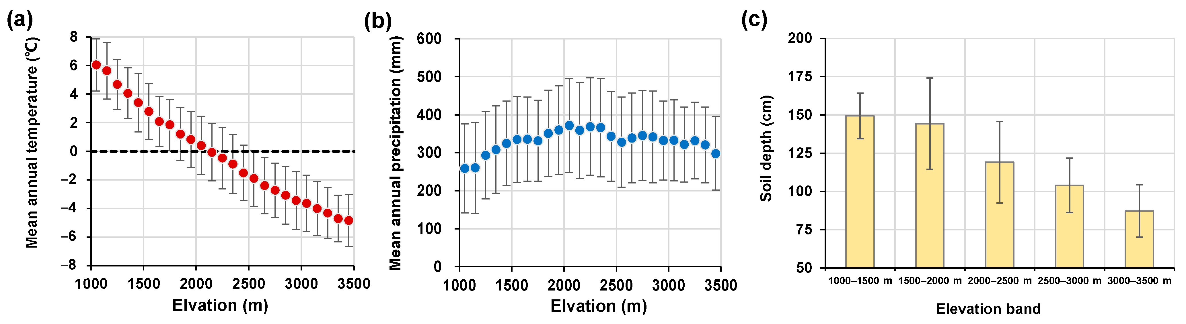
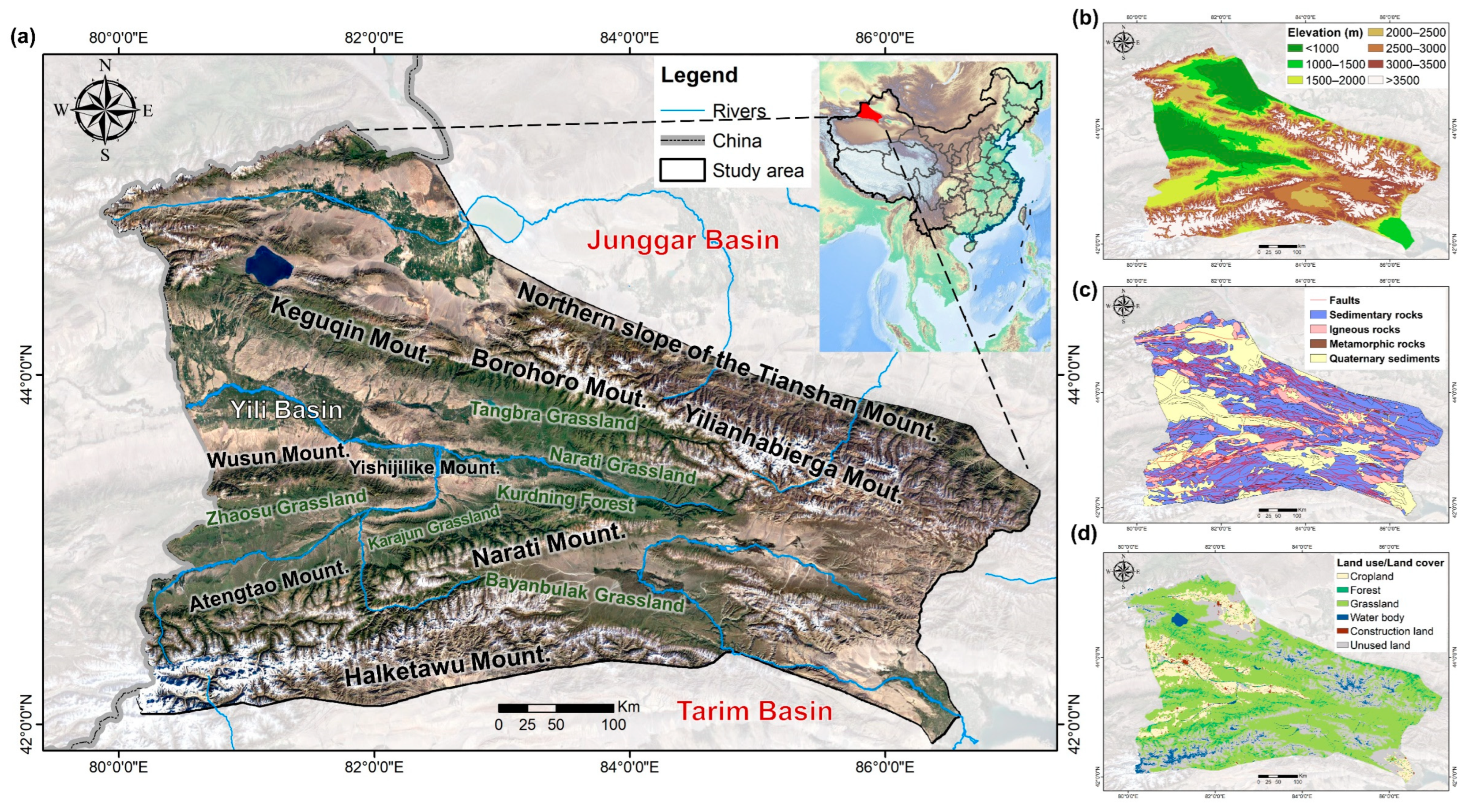
2.1. Study Area

The Tianshan Mountains are a large mountain range in Central Asia stretching approximately 2500 km in length and 200–400 km in width. It is the largest mountain chain and the largest isolated east-west mountain in the world’s temperate arid region, constituting a major segment of the southern part of the Central Asia Orogenic Belt. The Chinese segment of the Tianshan mountain range (its eastern portion), located in northwest China’s Xinjiang Uygur Autonomous Region, spans 1700 km from east to west, with an average elevation of approximately 2300 m above sea level (asl.) [27]. The Chinese Tianshan Mountains are geographically divided into eastern and western parts along the Urumqi-Korla line [28]. Our study focuses on the western part of Chinese Tianshan Mountains, CWTM (79°45′ E to 86°58′ E, 41°46′ N to 45°24′ N; Figure 1), which cover an area of approximately 248 × 103 km2 and include lofty mountains and steep hills, as well as broad intermountain basins and river valley plains (e.g., the Yili Basin). The CWTM extend across different bioclimatic zones, all belonging to a semi-arid climate, located between the Tarim Basin (warm–temperate desert) to the south and the Junggar Basin (temperate desert) to the north.
As a major part of the Tianshan Mountains, the CWTM have rich and diverse natural landscapes, such as glaciers, permanent snow cover, virgin forests, grasslands, and deserts, and thus form the most complete mountain altitudinal vegetation belts in a temperate arid region in the world. With the increase in altitude, it transitions into a montane steppe belt, a coniferous forest belt, an alpine meadow belt, an alpine cushion vegetation belt, and a nival belt [27]. The mean annual temperature is approximately 8 °C, and the mean annual precipitation varies from approximately 200 mm in the lower land to 500–700 mm in the mountain area, with most precipitation occurring during the wet season (June–September). The dominant vegetation type on the CWTM is grassland, including three grassland types: montane steppe, meadows, and desert steppe, consisting of Stipa capillata, Kobresia capillifolia, and Carex melanantha, respectively [29]. The major forest is the boreal forest Picea schrenkiana var. tianshannica. The main soil types of the western part of the Tianshan range are chernozems and kastanozems, with a thickness of generally <80 cm, derived from the soil parent material of uneven-thickness loess-like substances [30].
The Tianshan range is a classical resurgence orogenic belt produced by the far-field effects of the Indian–Eurasian continent collision, experiencing multi-stage episode uplift and deformation [31]. The Tianshan range is characterized by widely distributed active Cenozoic thrust faults, which present along the boundaries of all the basins [24]. The CWTM orogen is sandwiched between the Junggar Terrane to the north and the Tarim Block to the south. This orogen and its adjacent regions from north to south, including the Northern Tianshan Accretionary Complex, the Yili Block, the Central Tianshan Arc Terrane, and the Tarim Block, are separated by the North Tianshan Fault, the Nikolaev Line-North Nalati Fault, the Atbashi-Inylchek-South Nalati-Qawabulak Fault, and the North Tarim Fault, respectively [32]. Numerous active faults and folds are developed in the basin–mountain boundary zone and have caused highly fragmented rocks and a series of thrust earthquakes in these areas [25].

2.2. Data and Processing

Geological fault data were obtained from the 1:250,000 geological map provided by the GeoClound3.0 (https://geocloud.cgs.gov.cn) (Table 1). The 1:250,000 geological map contains fault line distribution with relevant attributes (i.e., fault segment length and style). A high density of faults indicates that the rock is relatively broken, and more fractures are conducive to the dissolution of carbonate rocks, thus accelerating the infiltration of water. Advanced spaceborne thermal emission and reflection radiometer (ASTER) global digital elevation model (DEM) data were downloaded from the Geospatial Data Cloud site (http://www.gscloud.cn/). The data were extracted and resampled with a spatial resolution of 90 m using a bilinear method to match the other datasets. Soil depth data with a spatial resolution of 1 km were extracted from a Chinese dataset of soil properties for land surface modeling (https://poles.tpdc.ac.cn/) [33].
This study used the China National Land Use and Cover Change (CNLUCC) dataset from the Resources and Environmental Sciences Data Center of the Chinese Academy of Sciences (http://www.resdc.cn/) [34]. The dataset was derived from the visual interpretation of Landsat Enhanced Thematic Mapper Plus (ETM+) images, with standard procedures and references to the well-established national land use and land cover remote sensing classification system. There are six land use and land cover categories in CNLUCC, including farmland, forestland, grassland, water, urban land, and unused land. Grassland is further classified into high-coverage (>50%), medium-coverage (20% to 50%), and low-coverage (5% to 20%) grassland according to the vegetation coverage. The classification accuracy of CNLUCC was validated using nationwide field verification. The CNLUCC dataset was shown to be suitable for conducting relevant long-term time series research due to its long time span, high data accuracy, and relatively higher accuracy when upscaled [35]. The CNLUCC data from 2000, 2005, 2010, 2015, and 2020 are averaged to represent the steady state of the regional cover.
To detect the spatial and temporal variations of vegetation growth in the study area, satellite-based NDVIs derived from a moderate resolution imaging spectroradiometer (MODIS) were employed. The MODIS-NDVI products named MOD13A2—with the spatial and temporal resolutions of 500 m and 16 days, respectively, from 2000 to 2020—were collected from Google Earth Engine (GEE). The monthly mean NDVI from April to October was used to calculate the annual growing season (GS) NDVI [29]. The Savitzky–Golay filter was used to eliminate the mixed noise in the image and improve the NDVI band quality [36].
Air temperature and precipitation data were obtained from the European Centre for Medium-Range Weather Forecast Reanalysis v5 (ERA5), which was relatively well constrained with satellite radiance observation through data assimilation. The temperature at 2 m and precipitation from January 2000 to December 2020 were extracted from the ERA5 dataset on the GEE online platform, then processed as an annual mean value for usage (shown in Figure A1).
Using the ArcGIS Desktop 10.8 (Esri Co. Ltd., Redlands, CA, USA), all the data were projected on the WGS 1984 coordinate system of the Mercator projection (Universal Transverse Mercator, UTM), and the index band was selected to be 45° N. The boundary of the CWTM was cropped to a unified range according to the previous section for processing and analysis. Through the fishing net tool in the ArcGIS software, multi grids with different sizes (1 km × 1 km, 2 km × 2 km, 3 km × 3 km, 5 km × 5 km, 10 km × 10 km) were created (Figure 2). Considering the size of forestland patches and the influence range of the faults, 3 km × 3 km grid units were chosen. For faults, the sum of fault lengths within each grid was counted, and the fault length density (FLD; their length (km) per km2, km/km2) within the grid was calculated; for LUCCs, the plurality within the grid cell was counted; and for the DEMs, NDVIs, meteorological elements, and environmental elements of soil properties, the mean value within the cell was counted. Extraction tools in the ArcGIS software were used to generate multiple attributes for individual grids, which were then analyzed, processed, and plotted in Microsoft Excel; some plots were drawn in Chiplot (https://www.chiplot.online/, accessed on 28 August 2023). Maps were drawn in the ArcGIS software.

2.3. Analysis Methods

2.3.1. Derivation of the Effect of the Individual Factor by the Boundary Line Approach

One environmental variable can be influenced jointly by many other variables, which limits the analysis and derivation of the relation between one dependent variable and one independent variable from the noncontrolled field data. To solve this problem, the boundary line approach (BLA) was developed, in which scatter plots are drawn between one dependent variable and each individual independent variable [37].

2.3.2. Correlation and Trend Analysis

Determination coefficients (R2) were used to analyze the correlation between the NDVI and elevation and year in this study. The Theil–Sen median (Sen’s slope estimation method) is a robust non-parametric statistical trend analysis method for evaluating the trend of long time series data [38]. This method has high computational efficiency and is insensitive to measurement error and discrete data, and it has been widely applied in the trend analysis of long time series. The Theil–Sen median can indicate the change trend of the NDVI in long time series at the pixel scale, and it can be calculated using the following formula:
S N D V I = M e d i a n N D V I j N D V I i j i , 2000 i < j 2020
where S N D V I is the value of the slope estimated by the Theil–Sen median; N D V I x is the value of the NDVI of each year in this study; and i and j are the different years between 2000 and 2020. When S N D V I > 0, it represents an uptrend, and when S N D V I < 0, it represents a downtrend.
The Mann–Kendall test is a nonparametric statistical test method that was first proposed by Mann in 1945 and further improved by Kendall and Sneyers. This test method has been widely used in trend significance tests of long time series data such as hydrological data, meteorological data, and climate data [38]. Trend index can be calculated using the following formulas:
Z = S 1 V ( S ) S > 0 0 S = 0 S + 1 V ( S ) S < 0
S = j = 1 n 1 i = j + 1 n s g n N D V I j N D V I i
s g n = 1 N D V I i N D V I j > 0 0 N D V I i N D V I j = 0 1 N D V I i N D V I j < 0
V S = n ( n 1 ) ( 2 n + 5 ) / 18
where Z is the standardized test statistic; n is the number of time series data, which is 21 in this study; and s g n indicates the function symbol. When n ≥ 8, the test statistic S is approximately normally distributed, and its mean and variance are as follows: if Z Z 1 α / 2 at an α level, it indicates that the assumption that there is no trend is rejected and there is an obvious trend change in the NDVI in the time series. Z 1 α / 2 is the value corresponding to the distribution table of the standard normal distribution function at the α confidence level. When Z > 1.65, Z >1.96, and Z > 2.58, it indicates that the trend passes the significance test of 90%, 95%, and 99%, respectively. We set α = 0.05 in this study (Table 2).

3. Results

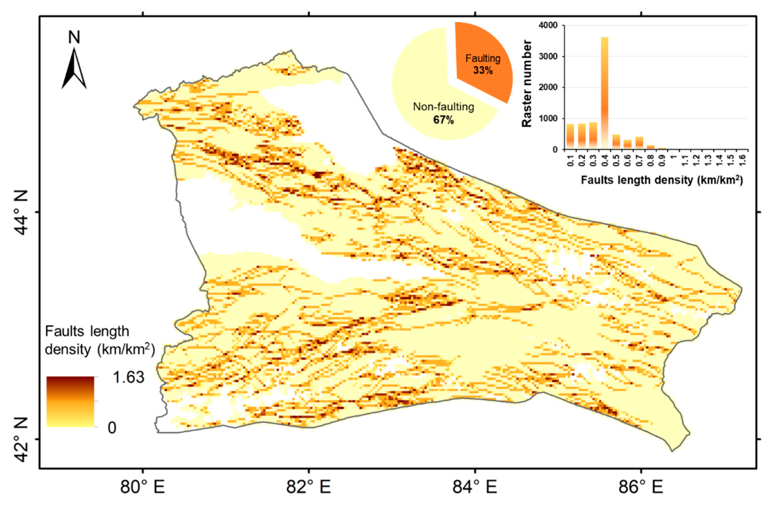
3.1. Spatial Distribution of Faults

3.1.1. Fault Length Density

Regional distribution of FLD provides a good representation of the fault direction in CWTM, with the principal fault directions observed being northwest–southeast and northeast–southwest (Figure 3). The faulting area accounts for 66.9% of the total area, whereas the non-faulting zone accounts for 33.1%. The faulting zone is further divided into subintervals based on FLD intervals of 0.01 km/km2. Within these intervals, the areas distributed among the ranges of 0–0.01 km/km2, 0.01–0.02 km/km2, and 0.02–0.03 km/km2 are similar, with grid cells ranging from 800 to 900. The interval of 0.3–0.4 km/km2 exhibits the highest peak, covering 32.7 × 10³ km2. As the FLD value exceeds 0.4 km/km2, the number of rasters decreases sequentially. The maximum FLD recorded is 1.63 km2, observed where 10 faults intersect.
The Jenks natural breaks classification method is a data classification technique designed to maximize the differences between classes. Using this method, the faulting zones are categorized into three classes: low-faulting, medium-faulting, and high-faulting, with corresponding FLD ranges of 0–0.25, 0.25–0.5, and >0.5 km/km2, respectively (Table 3). The respective areas covered by these classes are 1.8 km2, 3.9 km2, and 0.9 × 10⁴ km2. Among these, the medium-faulting zones have the largest area, accounting for 19.7% of the total region. The average FLD values for these classes are 0.10 km/km2, 0.33 km/km2, and 0.59 km/km2, with average elevations of 2361 m, 2427 m, and 2350 m, respectively. It is worth noting that the elevations of faulting zones are significantly higher than those of non-faulting zones.

3.1.2. Variation of FLD with Elevation

The distribution of low- and medium-faulting zones is not affected by variations in elevation, whereas the distribution of high-density faulting zone is closely related to elevation (Figure 4). Faulting zones with FLDs exceeding 1.4 km/km2 are primarily distributed at elevations of 2000–2500 m. The upper boundary line illustrates the relationship between FLD and elevation, with minimal influence from other factors. The maximum FLD in the study area exhibits an increasing-then-decreasing (convex) trend with elevation: it increases from 1 km/km2 at 1000 m to a peak value of 1.6 km/km2 around 2200 m, and then gradually decreases to 0.8 km/km2 at 3500 m. The study area is subsequently divided into 500 m elevation bands, and the percentages of faulting area are calculated for each band. Likewise, a higher faulting area percentage (%) appears at elevations of 2000–2500 m.

3.2. NDVI Variations

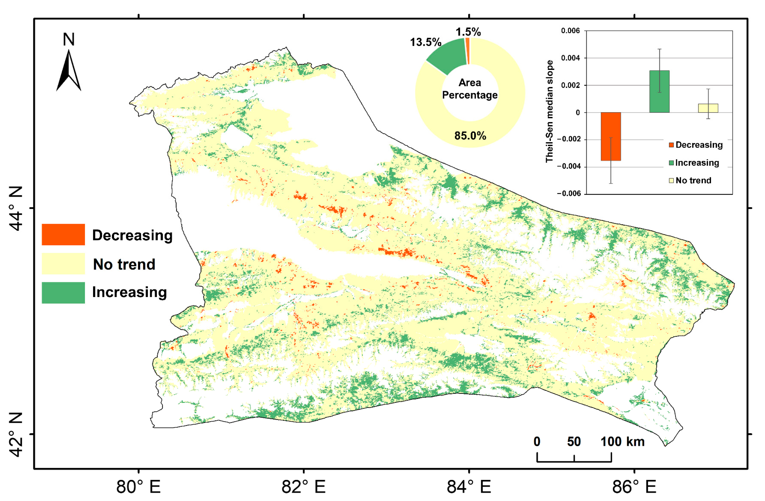
3.2.1. Spatio-Temporal Patterns of NDVI

Figure 5 shows the spatial distribution of multi-year mean NDVI values for forest and grass vegetation in the mid-altitude CWTM from 2000 to 2020. The results of hierarchical statistical analysis reveal that 27.1% of the area exhibits an NDVI of less than 0.3, whereas NDVI ranges from 0.3 to 0.5 for 40.5% of the area. Additionally, 32.4% of the area displays an NDVI value greater than 0.5. Due to the study area being located in a temperate arid and semi-arid climate, the spatial distribution of NDVI is significantly influenced by regional topographic and geomorphic factors. The low-vegetation zone primarily occupies lower-elevation areas distributed along the edges of the mountains. The medium-vegetation zone is predominantly found in the Bayanbulak Grassland and Keguqin Mountain. On the other hand, the high-vegetation zone is mainly located in the Tangbra Grassland on the southern slopes of the Borohoro Mountains (NW-SE trending), the forested areas of the mid-altitude mountains, including Wusun, Yishijilike, and Atengtao in the southern Yili Basin (near EW trend), as well as the Narati Grassland, Karajun Grassland, and Kurdning Forest on the northern slopes of the Narati and Halketawu Mountains. Notably, the high-coverage areas of the three zones correspond with the distribution of the principal faults, namely, the Kash River Fault, the North Wusunshan Fault, and the Narati Fault.
During the period from 2000 to 2020, the NDVI of forest and grass vegetation in the study area remained relatively constant, as shown in Figure 6. Zones with no apparent change covered 85.0% of the total area, with an average rate of change of 0.6 × 10⁻³ per year. Zones with a significant increase accounted for 13.5% of the total area and were mainly distributed in the northern slopes of the Tianshan, the Zhaosu Grassland, and the southern slopes of the Tianshan, with an average rate of change of 3.1 × 10⁻³ per year.. Additionally, 1.5% of the total area showed a significant decrease in NDVI, sporadically distributed in the grassland areas of the Keguqin Mountain and the Tangbra Grassland on the southern slope of the Borokonu Mountain, with an average rate of change of −3.5 × 10⁻³ per year.

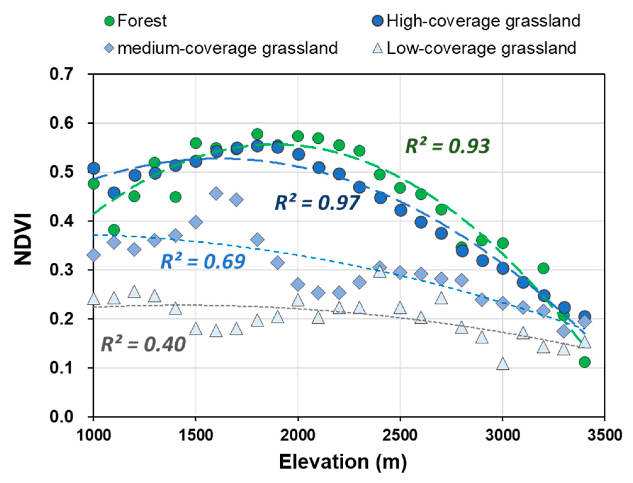
3.2.2. Relationship between NDVI Variation and Elevation

The mean multi-year NDVI values of different vegetation types exhibit a strong relationship with elevation (Figure 7). Both forest and high-coverage grassland display a convex distribution pattern, with NDVI values initially increasing and then decreasing with increasing elevation (R2 = 0.93 and 0.97, p < 0.01). The highest NDVI values for forest and high-coverage grassland are relatively similar at approximately 0.56. Moreover, the elevation bands corresponding to the maximum NDVI values are similar for both forest and grassland, located at elevations of 1800–2000 m. Grassland at higher elevations (>2000 m) present more sensitivity in NDVI changes compared to forested land. Medium-coverage grassland and low-coverage grassland exhibit relatively larger changes in NDVI with increasing elevation, but the overall trend indicates a decrease (R2 = 0.69 and 0.40, p < 0.05). Specifically, the NDVI of medium-coverage grassland decreases from 0.35 to 0.2 at 1000 m, whereas that of low-coverage grassland decreases from 0.24 to 0.15. Therefore, medium-covered grassland exhibits higher sensitivity to elevation changes.
The NDVI trends observed between 2000 and 2020 for different vegetation types are mainly characterized by no-change trends, and their distributions vary with elevation (Figure 8). In the case of forests, the percentage of area with an increasing NDVI trend significantly decreases with increasing elevation. Specifically, it decreases from 61.4% at relatively lower elevations of 1000–1500 m to 9.1% at higher elevations of 3000–3500 m. Conversely, the percentage of area exhibiting no significant change trend notably increases with increasing elevation. Regarding high-coverage and medium-coverage grasslands, the area with increasing NDVI values initially increases and then decreases with elevation. At elevations of 1500–2000 m, high-coverage grasslands reach their maximum NDVI value of 14%, whereas at higher elevations of 3000–3500 m, it decreases to 4%. Similarly, medium-coverage grasslands reach their maximum NDVI of 6.4% in the lower middle elevation zone and decrease to 2% at higher elevations of 3000–3500 m, demonstrating relative insensitivity to elevation variation. As for low-coverage grasslands, the percentage of areas with an increasing NDVI trend is highest (17%) at lower elevations of 1500–2000 m, whereas it remains low (<10%) in all other higher elevation zones.

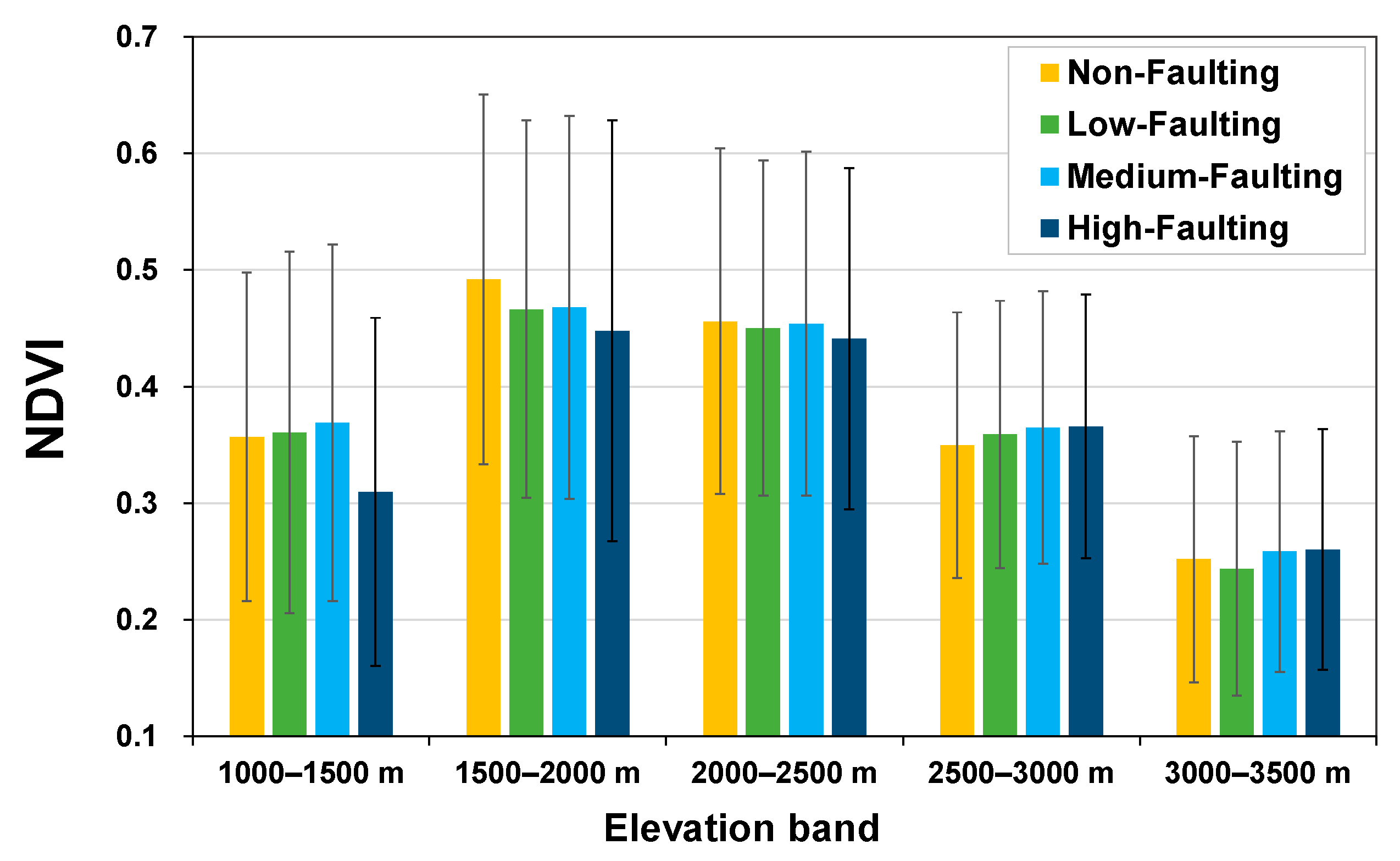
3.3. Elevation-Dependent Relationship between NDVI Variation and FLD

Multi-year mean vegetation NDVI of different faulting classes in various elevation bands shows certain variations (Figure 9). At elevations of 1000–1500 m, the NDVI is higher in the low-faulting and medium-faulting zones compared to the non-faulting zone, while it is lowest in the high-faulting zone. At elevations of 1500–2000 m, the NDVI in the faulting zone is lower than that in the non-faulting zone. At elevations of 2000–2500 m, the NDVI value is similar in the non-faulting, low-faulting, and medium faulting zones, while it is lowest in the high-faulting zone. At elevations of 2500–3500 m, the NDVI is higher in the faulting zone compared to the non-faulting zone. Therefore, the influence of fault development on vegetation growth varies along the elevation gradient.
Elevation influences the interannual variability in NDVI within different faulting zones (Figure 10). Across all elevation subzones, the multi-year NDVI exhibits a non-significant increasing trend (p > 0.05). At elevations of 1000–2500 m, the NDVI is lower in the faulting zone compared to the non-faulting zone. Conversely, at elevations of 2500–3500 m, the NDVI is higher in the faulting zone compared to the non-faulting zone. It is important to note that the presence of faults does not alter the multi-year trend in NDVI.
Different fault densities have varying impacts on the trends of NDVI variation across different elevations and vegetation types (Figure 11). Notably, forests with decreasing NDVI trends are consistently located at elevations below 2500 m. The percentage of area with increasing NDVI trends within this elevation range decreases progressively with increasing fault density, reaching its lowest value (<10%) in regions characterized by a high fault density. Conversely, for forests at elevations above 2500 m, the highest percentage of areas with increasing NDVI trends (accounting for 60%) is found in regions characterized by a high density of faults. For grasslands, areas with decreasing NDVI trends are predominantly located at elevations below 2500 m. The density of faults did not significantly affect the variation in vegetation state.

4. Discussion

4.1. Elevational Patterns of Vegetation Growth and Its Links with Tectonic Faults

The Tianshan region constitutes the principal ecological barrier in the arid northwest of China, characterized by its complete mountain altitudinal vegetation belts and complex geological and geomorphological setting. Previous studies showed that the elevational patterns of vegetation are caused by differences in temperature, humidity, radiation intensity, soil properties, and human activities [39]. With increasing elevation, temperature and soil depth usually decrease, whereas precipitation follows a trend of initially increasing and subsequently slightly decreasing (Figure A1). Additionally, the transition of vegetation types progresses gradually from desert to montane steppe, coniferous forest, and alpine meadow [27]. These dynamic factors exhibit regular variation along the vertical axis, thereby shaping the formation of altitudinal vegetation belts.
This investigation highlighted that the vegetation growth (characterized by NDVI) of forests and high-coverage grasslands within the CWTM region displays a unimodal (or convex) pattern that increases and then decreases as elevation increases (Figure 5 and Figure 7). NDVI reaches its peak value at an elevation of 1800–2000 m and subsequently decreases. This elevation-associated unimodal pattern is consistent with previous research in mountain ecology, both through ground surveys and remote sensing [39,40]. Nevertheless, the elevation distribution of the NDVI peak is slightly different from that of the nearby dryland mountains. For example, the highest NDVI elevation zone of the Altai Mountains in the north is 2100–2200 m [41], whereas that of the Qilian Mountains in the east is 2700–3200 m [42]. This difference may be attributed to variations in climate zones, soil zones, regional atmospheric water vapor, mountain heights, and slope orientations [40]. Besides, this study indicated that the NDVI of medium- and low-coverage grasslands in the CWTM showed a general decreasing trend with increasing elevation, consistent with the results of previous studies on grasslands in the mid-altitude Qinling Mountains [43].
According to our results, the elevation zones of optimal forest and high-coverage grassland are basically consistent with the high faulting zone, which are all around an elevation of 2000 m (Figure 4 and Figure 7). This consistency in vegetation growth and the high-density fault zone distribution has been less frequently reported in previous studies, most of which focus on the impact of climatic factors (such as temperature and precipitation) or human activities to vegetation variations [44,45]. In accordance with the present findings, a previous study conducted along a 3000 m elevation gradient with tectonic faults on the Tibetan Plateau (Galongla and Gongga Mountains) showed that the elevational breakpoints (2000–2800 m asl.) of biological communities and ecosystem functions surprisingly coincided with the locations of faults [10]. This research also indicated that, across the Indus-Yalu suture zone fault in southwestern Tibet, most chemical characteristics, including minerals, weathering indices, and soil properties, were significantly different. This difference could be explained by the phenomenon that active faulting leads to the exposure of buried bedrock, which then can be physically and chemically weathered to produce mineral-rich soils [46]. Hence, this consistency may have some eco-geological significance that should be validated through further field surveys.

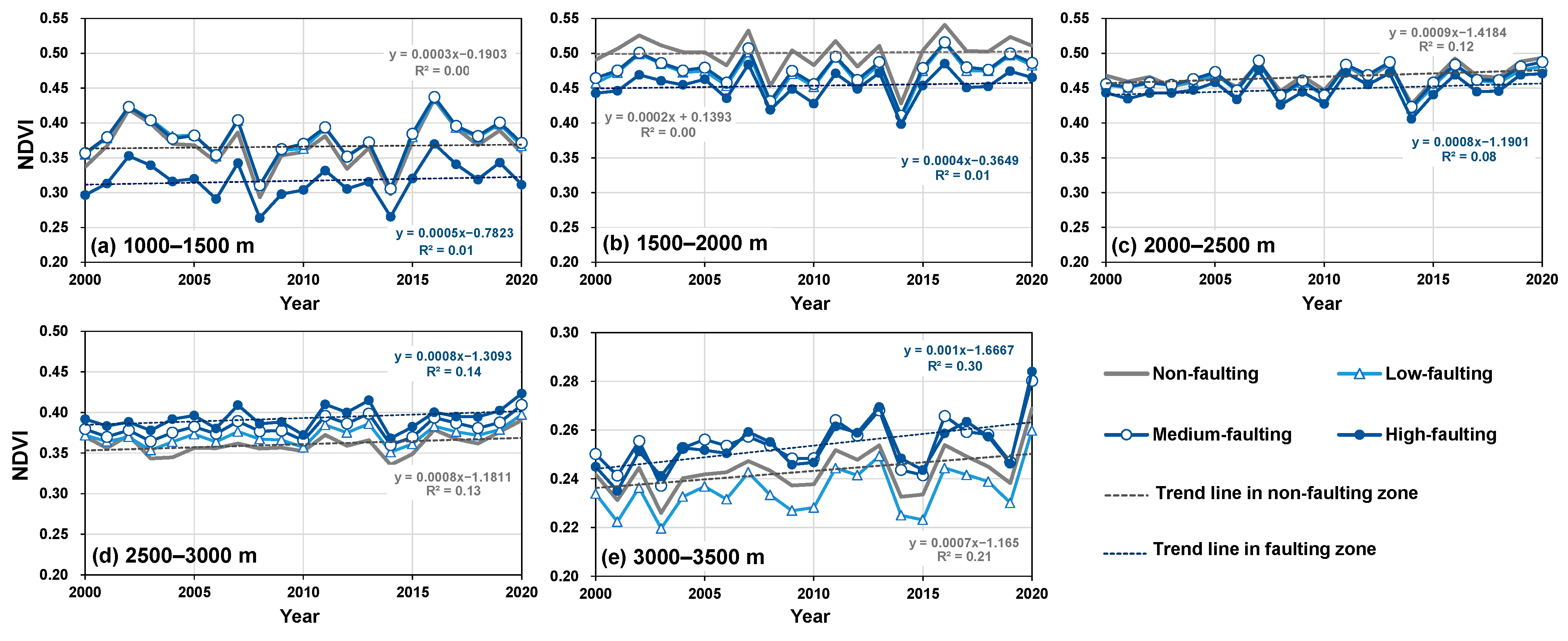
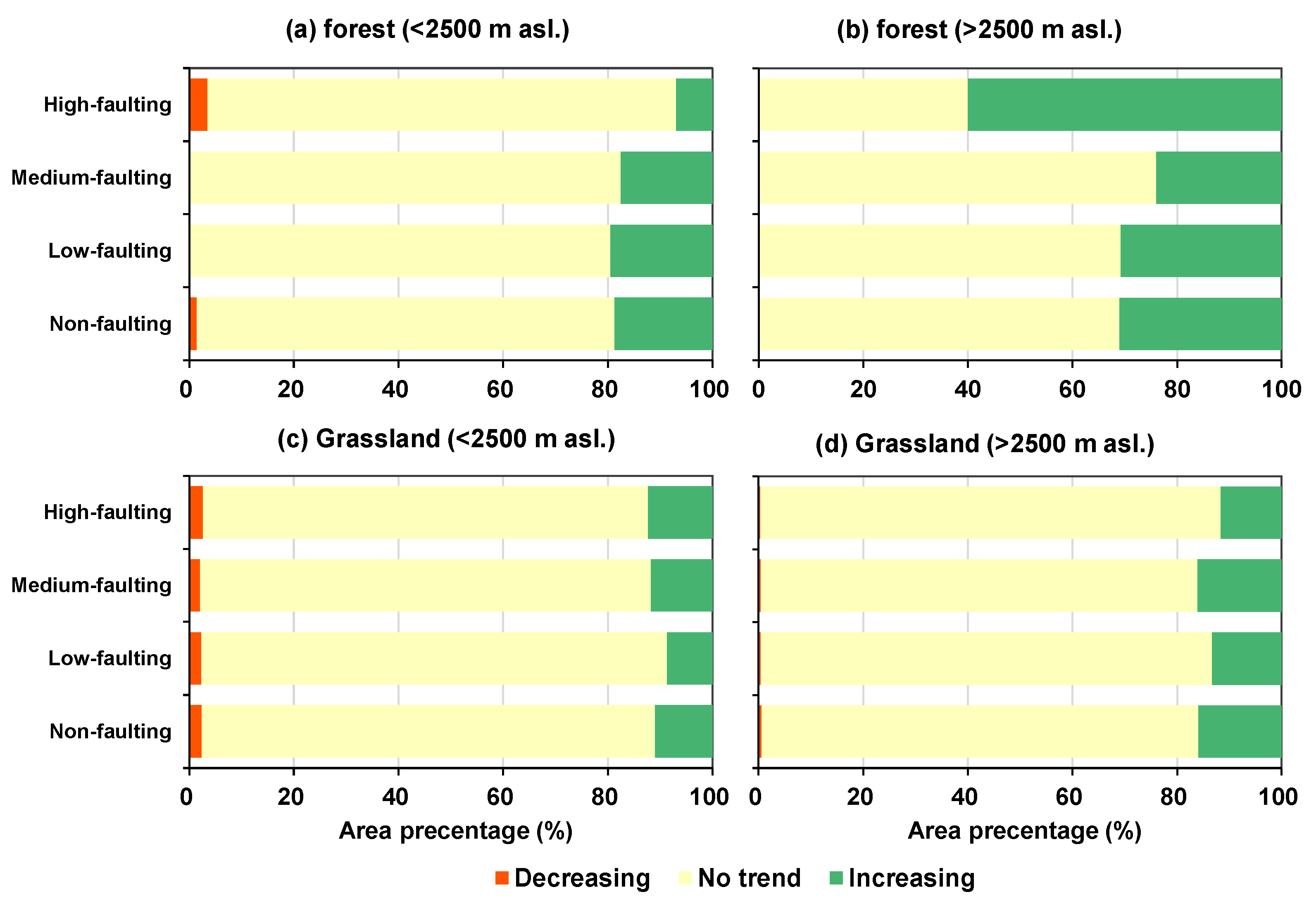
4.2. Temporal Variations of Vegetation Growth

This study revealed that the area with no trend of vegetation variation in the study area covered almost 90% of the total area (Figure 6). In contrast, recent research has highlighted the browning of vegetation on the Tianshan during the period from 1998 to 2015, attributing this phenomenon to soil water deficits [25]. This inconsistency could be explained by the fact that precipitation in the study region has increased since 2015, and Northwestern China experienced a “warming-wetting” trend in recent years [47]. The increased precipitation in recent years implies that the intensified interannual variability of precipitation has complicated the trend in vegetation variation [48].
Notably, the area with a significant greening trend, which accounted for approximately 10% of the total area, was predominantly located on the northern slopes of North Tianshan (Figure 6). This result is consistent with previous research and is mainly attributed to climate change [49]. Furthermore, it is important to highlight the influence of elevation on vegetation state. For example, the proportion of improved forest area showed a notable decrease as elevation increased (Figure 8). This observation could potentially be linked to human activities, such as the application for UNESCO World Heritage Site status of the Tianshan, which was initiated in 2010 and concluded in 2013 [49]. Interestingly, our results were consistent with a previous study indicating that the strongest positive NDVI trends occurred at lower elevations, which could be attributed to vegetation restoration activities [50]. In contrast, the area with the most degraded vegetation is also located at low-elevation regions, primarily in the grassland surrounding the Yili Basin (Figure 6 and Figure 11). Notably, the decreasing rate of the NDVI in these regions was notably high (Figure 6), suggesting that overgrazing may continue to be a challenge in this area [51]. These results suggested that human activities had a significant effect on vegetation growth in the low-elevation region.

4.3. Elevation-Dependent Contrasting Effects of Fault Distribution on Vegetation Growth

The results indicated that the NDVI of the faulting zone in the elevation range of 1000–2500 m is lower compared to the non-faulting zone, whereas that of the faulting zone in the elevation range of 2500–3500 m is higher (Figure 9). This phenomenon is particularly significant for forests and could be attributed to changes in fault-induced slope instability and hydrothermal conditions.
Ecological disturbances resulting from fault-induced landslides can exhibit variations along the elevation gradient. Disadvantageous ecological effects of tectonic events have been addressed. In southern Chile and New Zealand, the effects of tectonic disturbances, especially those associated with strong earthquakes, play a crucial role in determining forest structure and composition [20]. These landslide-related disturbances (e.g., earthquake-triggered mass movements) impact plant communities directly, causing damage to plant biomass by either killing entire plants or removing parts of them, which is particularly severe within faulting zones [22]. Previous studies have shown that earthquake-induced landslides within active fault zones have led to significant losses in local vegetation net primary productivity [52,53]. In comparison to higher elevations, bedrock in lower-elevation slopes within fault zones undergoes more pronounced physical and chemical weathering [54]. This process increases rock fracture and porosity, augments regolith thickness, and enhances slope instability and susceptibility to landslides [55]. Notably, a previous study showed that fault-induced landslides in the CWTM region were concentrated in the elevation range of 1000–2500 m. Specifically, there were 602, 814, and 78 incidents recorded at 1000–1500 m, 1500–2000 m, and 2000–2500 m, respectively [56]. In contrast, the total number of fault-induced landslides occurring in the 2500–3500 m elevation range was less than 30. Consequently, ecosystems in lower-elevation slopes (<2500 m asl.) within fault zones experience higher levels of disturbance, including an increased risk of tree falls. These areas face challenges in achieving normal ecological succession, resulting in lower vegetation cover.
Meanwhile, faulting can result in the rapid incision of valleys and the erosion of hillslopes. These changes not only alter local humidity and thermal conditions but also give rise to “catenas,” which are sequences of soil variations extending from hilltop to middle slope and the valley bottom [17,57]. Vegetation experiences differences in insulation, wind shear, and local evapotranspiration between hilltops and valleys, which could affect vegetation growth [58]. Within fault valleys at higher elevations (>2500 m asl.), water and soil accumulate, and there is limited heat exchange compared to the other hillslope positions (e.g., ridge) [59]. As a result, vegetation flourishes in the fault-induced valley. Previous study found that the mean forest carbon loading consistently decreased from valley bottoms to ridges [60]. Notably, faults in the study area predominantly exhibit an east-west orientation, leading to the formation of north-facing shaded slopes and south-facing sunny slopes [61]. The slope aspect significantly influences microclimate factors, including air and soil temperature, evapotranspiration, and wind speed [12]. In the northern hemisphere, north-facing slopes exhibit higher biomass, greater coverage, and increased vegetation height compared to south-facing slopes [60]. Consequently, the formation of fault valleys contributes to enhanced vegetation growth.
Moreover, the presence of fault-induced valleys, characterized by reductions in elevation, could have contrasting impacts on vegetation along the elevation gradient. Since vegetation growth exhibits a unimodal distribution (shown in Figure 7, with the peak value around 2000 m asl.) Reductions in elevation at lower elevations (<2000 m asl.) could lead to a deviation from the optimal environmental conditions. In contrast, reductions in elevation could have more advantageous effects on vegetation growth at higher elevations (>2000 m asl.) of the NDVI-elevation unimodal curve.
Previous studies have illustrated the beneficial ecological effects of tectonic phenomena in tectonic river basins. For example, a local-scale study in a semi-arid fault-controlled river basin in Africa (~1500 m asl.) indicated that active normal faulting is an important factor in stabilizing vegetation growth patterns, which creates favorable hydrological and pedological conditions along the escarpment [17]. Tectonic basin and associated alluvial fan (~1000 m asl.) contain porous aeolian sands and a significant number of transported fines, indicating its potential for groundwater buffering [23]. This fault-induced landscape serves as an environmental hydro-refugia for local vegetation. Consistent with the literature, this research suggested that fault valleys in high-elevation mountains could also serve as environmental refugia for local vegetation.
Notably, thermal anomalies associated with faults have been detected in previous studies [62]. The average land surface temperature in the central zone of active faults is 1° higher than the surrounding environment within a certain distance of approximately 5 km [63]. In particular, permeable structures such as faults exercise a primary control on local fluid flow patterns, with most upflow zones residing in complex fault interaction zones [64]. Most intermediate- (≥125 °C) to high-temperature (≥225 °C) geothermal systems reside along normal faults in complex interaction zones.
Therefore, the effects of faults on local habitats vary along the elevation gradient. At lower elevations (1000–2500 m asl.), vegetation in fault zones experiences reduced growth due to increased ecological disturbance caused by landslides. In contrast, the incidence of geohazards in faulting zones at higher elevations (2500–3500 m asl.) is significantly reduced. Meanwhile, fault valleys provide favorable accommodation space for vegetation in high-altitude landscapes, creating improved hydrothermal conditions for growth. Furthermore, thermal anomalies within fault zones may help mitigate temperature stress on vegetation in high-elevation, temperature-limited areas.
Our findings corroborate previous studies on the relationship between alpine ecosystem functions and geological events. For example, the inclusion of geological factors, such as parent rock and weathering, increased the explained variations in plant communities and ecosystem functions in the southeastern Tibetan Plateau by 67.9% and 27.6%, respectively [10]. Geological conditions, such as bedrock lithology and erodibility, strongly affect local soil thickness and water storage capacity, which in turn determine the distribution and seasonal stability of vegetation [65]. Further fieldwork and research would be required to obtain a deeper understanding of the influence of tectonic activity on hydrological, pedological, and biological properties in sensitive ecosystems within tectonically active landscapes.

5. Conclusions

Collectively, this study investigated the distribution and dynamics of NDVI in the mid-altitude region of the CWTM, and their relationships with tectonic fault length density at different elevation zones. The NDVI of forests and high-coverage grasslands exhibited a convex distribution along the elevation gradient. The elevation of the high-density faulting zone was consistent with the peak value of forests and high-coverage grasslands, both of which were located at elevations around 2000 m. There were obvious differences in the effects of FLD on vegetation variation at different elevation zones: FLD had a negative effect on NDVI in the water-limited zone at elevations of 1000–2500 m, whereas it enhanced NDVI in the temperature-limited zone at 2500–3500 m (particularly for forests). This elevation-dependent contrasting effect of faults on vegetation growth could be attributed to the more favorable hydrothermal conditions for vegetation in fault-induced geomorphology and the reduced susceptibility to landslides with increasing elevation. This study has important implications for understanding how tectonics control the alpine ecosystem in tectonically active, dryland mountains, revealing the diversity and complexity of the geology–environment relationship. Further field-based studies on the lithology of bedrock, as well as terrain attributes in the faulting zone, would provide a better understanding of the effects of tectonic activities on vegetation growth.

Author Contributions

Conceptualization, X.L. (Xiaohuang Liu) and J.L.; data curation, analysis, and methodology, H.L. and X.L. (Xinping Luo); visualization, R.W. and L.X.; writing—original draft preparation, and editing, H.L., X.Z. and W.Z. All authors have read and agreed to the published version of the manuscript.

Funding

This research was supported by the project of China Geological Survey (grant No. DD20230514), and the Third Xinjiang Scientific Expedition Program (grant No. 2022xjkk090405 and 2021xjkk1401).

Data Availability Statement

The data presented in this study are available from the corresponding author X.L. with a reasonable request. The data are not publicly available due to privacy restrictions.

Acknowledgments

We thank the reviewers for their thoughtful comments and constructive suggestions which substantially improved this manuscript.

Conflicts of Interest

The authors declare no conflict of interest.

Appendix A

Figure A1. (a) Mean annual temperature, (b) precipitation and (c) soil depth varies along elevational gradients on the CWTM (error bars represent the standard deviation).
Forests 14 02336 g0a1

References

  1. Gao, W.; Zheng, C.; Liu, X.; Lu, Y.; Chen, Y.; Wei, Y.; Ma, Y. NDVI-based vegetation dynamics and their responses to climate change and human activities from 1982 to 2020: A case study in the Mu Us Sandy Land, China. Ecol. Indic. 2022, 137, 108745. [Google Scholar] [CrossRef]
  2. Chen, Z.; Wang, W.; Fu, J. Vegetation response to precipitation anomalies under different climatic and biogeographical conditions in China. Sci. Rep. 2020, 10, 830. [Google Scholar] [CrossRef] [PubMed]
  3. Sun, G.; Li, L.; Li, J.; Liu, C.; Wu, Y.; Gao, S.; Wang, Z.; Feng, G. Impacts of climate change on vegetation pattern: Mathematical modelling and data analysis. Phys. Life Rev. 2022, 42, 239–270. [Google Scholar] [CrossRef] [PubMed]
  4. Wang, J.; Hu, A.; Meng, F.; Zhao, W.; Yang, Y.; Soininen, J.; Shen, J.; Zhou, J. Embracing mountain microbiome and ecosystem functions under global change. New Phytol. 2022, 234, 1987–2002. [Google Scholar] [CrossRef] [PubMed]
  5. Antonelli, A.; Kissling, W.D.; Flantua, S.A.; Bermúdez, M.A.; Mulch, A.; Muellner-Riehl, A.N.; Kreft, H.; Linder, H.P.; Badgley, C.; Fjeldså, J.; et al. Geological and climatic influences on mountain biodiversity. Nat. Geosci. 2018, 11, 718–725. [Google Scholar] [CrossRef]
  6. Dong, Y.; Shi, X.; Sun, S.; Sun, J.; Hui, B.; He, D.; Chong, F.; Yang, Z. Co-evolution of the Cenozoic tectonics, geomorphology, environment and ecosystem in the Qinling Mountains and adjacent areas, Central China. Geosyst. Geoenviron. 2022, 1, 100032. [Google Scholar] [CrossRef]
  7. Dong, X.; Martin, J.B.; Cohen, M.J.; Tu, T. Bedrock mediates responses of ecosystem productivity to climate variability. Commun. Earth Environ. 2023, 4, 114. [Google Scholar] [CrossRef]
  8. Graham, R.; Rossi, A.; Hubbert, R. Rock to regolith conversion: Producing hospitable substrates for terrestrial ecosystems. GSA today 2010, 20, 4–9. [Google Scholar] [CrossRef]
  9. Ding, W.; Ree, R.; Spicer, R.; Xing, Y. Ancient orogenic and monsoon-driven assembly of the world’s richest temperate alpine flora. Science 2020, 369, 578–581. [Google Scholar] [CrossRef]
  10. Hu, A.; Wang, J.; Sun, H.; Niu, B.; Si, G.; Wang, J.; Yeh, C.; Zhu, X.; Lu, X.; Zhou, J.; et al. Mountain biodiversity and ecosystem functions: Interplay between geology and contemporary environments. ISME J. 2020, 14, 931–944. [Google Scholar] [CrossRef]
  11. Fan, Y.; Clark, M.; Lawrence, D.; Swenson, S.; Band, L.E.; Brantley, S.; Brooks, P.; Dietrich, W.; Flores, A.; Grant, G.; et al. Hillslope hydrology in global change research and earth system modeling. Water Resour. Res. 2019, 55, 1737–1772. [Google Scholar] [CrossRef]
  12. Yang, J.; El-Kassaby, Y.A.; Guan, W. The effect of slope aspect on vegetation attributes in a mountainous dry valley, Southwest China. Sci. Rep. 2020, 10, 16465. [Google Scholar] [CrossRef] [PubMed]
  13. Dawson, T.E.; Hahm, W.J.; Crutchfield-Peters, K. Digging deeper: What the critical zone perspective adds to the study of plant ecophysiology. New Phytol. 2020, 226, 666–671. [Google Scholar] [CrossRef] [PubMed]
  14. Hahm, W.J.; Riebe, C.S.; Lukens, C.E.; Araki, S. Bedrock composition regulates mountain ecosystems and landscape evolution. Proc. Natl. Acad. Sci. USA 2014, 111, 3338–3343. [Google Scholar] [CrossRef] [PubMed]
  15. Hahm, W.J.; Rempe, D.M.; Dralle, D.N.; Dawson, T.E.; Dietrich, W.E. Oak transpiration drawn from the weathered bedrock vadose zone in the summer dry season. Water Resour. Res. 2020, 56, e2020WR027419. [Google Scholar] [CrossRef]
  16. Jiménez-Rodríguez, C.D.; Sulis, M.; Schymanski, S. Exploring the role of bedrock representation on plant transpiration response during dry periods at four forested sites in Europe. Biogeosciences 2020, 19, 3395–3423. [Google Scholar] [CrossRef]
  17. Ludat, A.L.; Kübler, S. Tectonic controls on the ecosystem of the Mara River basin, East Africa, from geomorphological and spectral index analysis. Biogeosciences 2023, 20, 1991–2012. [Google Scholar] [CrossRef]
  18. Shlemon, R.J.; Riefner, R.E. The Role of Tectonic Processes in the Interaction between Geology and Ecosystems, In Geology and Ecosystems, 1st ed.; Zektser, I.S., Marker, B., Ridgway, J., Rogachevskaya, L., Vartanyan, G., Eds.; Springer: Boston, MA, USA, 2006; pp. 49–60. [Google Scholar]
  19. Dixon, J.L.; Hartshorn, A.S.; Heimsath, A.M.; DiBiase, R.A.; Whipple, K.X. Chemical weathering response to tectonic forcing: A soils perspective from the San Gabriel Mountains, California. Earth Planet. Sci. Lett. 2012, 323, 40–49. [Google Scholar] [CrossRef]
  20. Veblen, T.T.; González, M.E.; Stewart, G.H.; Kitzberger, T.; Brunet, J. Tectonic ecology of the temperate forests of South America and New Zealand. N. Z. J. Bot. 2006, 54, 223–246. [Google Scholar] [CrossRef]
  21. Kübler, S.; Rucina, S.; Aßbichler, D.; Eckmeier, E.; King, G. Lithological and topographic impact on soil nutrient distributions in tectonic landscapes: Implications for Pleistocene human-landscape interactions in the southern Kenya Rift. Front. Environ. Sci. 2021, 9, 103. [Google Scholar] [CrossRef]
  22. Duan, Y.; Di, B.; Ustin, S.L.; Xu, C.; Xie, Q.; Wu, S.; Li, J.; Zhang, R. Changes in ecosystem services in a montane landscape impacted by major earthquakes: A case study in Wenchuan earthquake-affected area, China. Ecol. Indic. 2021, 126, 107683. [Google Scholar] [CrossRef]
  23. Reynolds, S.C.; Marston, C.G.; Hassani, H.; King, G.C.; Bennett, M.R. Environmental hydro-refugia demonstrated by vegetation vigour in the Okavango Delta, Botswana. Sci. Rep. 2016, 6, 35951. [Google Scholar] [CrossRef] [PubMed]
  24. Li, J.; Zhang, J.; Zhao, X.; Jiang, M.; Li, Y.; Zhu, Z.; Feng, Q.; Wang, L.; Sun, G.; Liu, J.; et al. Mantle subduction and uplift of intracontinental mountains: A case study from the Chinese Tianshan Mountains within Eurasia. Sci. Rep. 2016, 6, 28831. [Google Scholar] [CrossRef] [PubMed]
  25. Li, W.; Chen, Y.; Yuan, X.; Xiao, W.; Windley, B.F. Intracontinental deformation of the Tianshan Orogen in response to India-Asia collision. Nat. Commun. 2022, 13, 3738. [Google Scholar] [CrossRef] [PubMed]
  26. Yao, Y.; Wen, S.; Yang, L.; Wu, C.; Sun, X.; Wang, L.; Zhang, Z. A shallow and left-lateral rupture event of the 2021 Mw 5.3 Baicheng earthquake: Implications for the diffuse deformation of southern Tianshan. Earth Space Sci. 2022, 9, e2021EA001995. [Google Scholar] [CrossRef]
  27. Zhang, W.; Luo, G.; Chen, C.; Ochege, F.; Hellwich, O.; Zheng, H.; Hamdi, R.; Wu, S. Quantifying the contribution of climate change and human activities to biophysical parameters in an arid region. Ecol. Indic. 2021, 129, 107996. [Google Scholar] [CrossRef]
  28. Ni, X.; Wang, B.; Cluzel, D.; Liu, J.; He, Z. Late Paleozoic tectonic evolution of the North Tianshan Belt: New structural and geochronological constraints from meta-sedimentary rocks and migmatites in the Harlik Range (NW China). J. Asian Earth Sci. 2021, 210, 104711. [Google Scholar] [CrossRef]
  29. Li, Y.; Chen, Y.; Sun, F.; Li, Z. Recent vegetation browning and its drivers on Tianshan Mountain, Central Asia. Ecol. Indic. 2021, 129, 107912. [Google Scholar] [CrossRef]
  30. Tudi, M.; Li, H.; Li, H.; Wang, L.; Yang, L.; Tong, S.; Yu, Q.J.; Ruan, H.D. Evaluation of soil nutrient characteristics in Tianshan Mountains, North-western China. Ecol. Indic. 2022, 143, 109431. [Google Scholar] [CrossRef]
  31. Liu, X.; Yuan, S.; Bai, X.; Jiang, J.; Li, Y.; Liu, J. Tectonic uplift of the Tianshan Mountains since Quaternary: Evidence from magnetostratigraphy of the Yili Basin, northwestern China. Int. J. Earth Sci. 2023, 112, 855–865. [Google Scholar] [CrossRef]
  32. Luo, W.; Zhang, Z.; Duan, S.; Jiang, Z.; Wang, D.; Chen, J.; Sun, J. Geochemistry of the Zhibo submarine intermediate-mafic volcanic rocks and associated iron ores, Western Tianshan, Northwest China: Implications for ore genesis. Geol. J. 2018, 53, 3147–3172. [Google Scholar] [CrossRef]
  33. Shangguan, W.; Dai, Y.; Liu, B.; Zhu, A.; Duan, Q.; Wu, L.; Ji, D.; Ye, A.; Yuan, H.; Zhang, Q.; et al. A China Dataset of Soil Properties for Land Surface Modeling. J. Adv. Model. Earth Syst. 2013, 5, 212–224. [Google Scholar] [CrossRef]
  34. Liu, J.; Kuang, W.; Zhang, Z.; Xu, X.; Qin, Y.; Ning, J.; Zhou, W.; Zhang, S.; Li, R.; Yan, C.; et al. Spatiotemporal characteristics, patterns, and causes of land-use changes in China since the late 1980s. J. Geogr. Sci. 2014, 24, 195–210. [Google Scholar] [CrossRef]
  35. He, S.; Li, J.; Wang, J.; Liu, F. Evaluation and analysis of upscaling of different land use/land cover products (FORM-GLC30, GLC_FCS30, CCI_LC, MCD12Q1 and CNLUCC): A case study in China. Geocarto Int. 2022, 37, 17340–17360. [Google Scholar] [CrossRef]
  36. Li, H.; Luo, Y.; Sun, L.; Li, X.; Ma, C.; Wang, X.; Jiang, T.; Zhu, H. Modelling the artificial forest (Robinia pseudoacacia L.) root–soil water interactions in the Loess Plateau, China. Hydrol. Earth Syst. Sci. 2022, 26, 17–34. [Google Scholar] [CrossRef]
  37. Yang, W.; Wang, Y.; Webb, A.A.; Li, Z.; Tian, X.; Han, Z.; Wang, S.; Yu, P. Influence of climatic and geographic factors on the spatial distribution of Qinghai spruce forests in the dryland Qilian Mountains of Northwest China. Sci. Total. Environ. 2018, 612, 1007–1017. [Google Scholar] [CrossRef]
  38. Gao, X.; Huang, X.; Lo, K.; Dang, Q.; Wen, R. Vegetation responses to climate change in the Qilian Mountain Nature Reserve, Northwest China. Glob. Ecol. Conserv. 2021, 28, e01698. [Google Scholar] [CrossRef]
  39. Xiong, Y.; Wang, H. Spatial relationships between NDVI and topographic factors at multiple scales in a watershed of the Minjiang River, China. Ecol. Inform. 2022, 69, 101617. [Google Scholar] [CrossRef]
  40. Zou, L.; Tian, F.; Liang, T.; Eklundh, L.; Tong, X.; Tagesson, T.; Dou, Y.; He, T.; Liang, S.; Fensholt, R. Assessing the upper elevational limits of vegetation growth in global high-mountains. Remote Sens. Environ. 2023, 286, 113423. [Google Scholar] [CrossRef]
  41. Tai, X.; Epstein, H.E.; Li, B. Elevation and climate effects on vegetation greenness in an arid mountain-basin system of Central Asia. Remote Sens. 2020, 12, 1665. [Google Scholar] [CrossRef]
  42. Fu, J.X.; Cao, G.C.; Guo, W.J. Changes of growing season NDVI at different elevations, slopes, slope aspects and its relationship with meteorological factors in the southern slope of the Qilian Mountains, China from 1998 to 2017. J. Appl. Ecol. 2020, 31, 1203–1212, (In Chinese with English abstract). [Google Scholar] [CrossRef]
  43. Huang, C.; Yang, Q.; Guo, Y.; Zhang, Y.; Guo, L. The pattern, change and driven factors of vegetation cover in the Qin Mountains region. Sci. Rep. 2020, 10, 20591. [Google Scholar] [CrossRef] [PubMed]
  44. Zhang, Y.; Liu, L.Y.; Liu, Y.; Zhang, M.; An, C.B. Response of altitudinal vegetation belts of the Tianshan Mountains in northwestern China to climate change during 1989–2015. Sci. Rep. 2021, 11, 4870. [Google Scholar] [CrossRef] [PubMed]
  45. Wei, Y.; Lu, H.; Wang, J.; Wang, X.; Sun, J. Dual influence of climate change and anthropogenic activities on the spatiotemporal vegetation dynamics over the Qinghai-Tibetan plateau from 1981 to 2015. Earth’s Future 2022, 10, e2021EF002566. [Google Scholar] [CrossRef]
  46. Wei, Z.; He, H. Weathering history of an exposed bedrock fault surface interpreted from its topography. J. Struct. Geol. 2013, 56, 34–44. [Google Scholar] [CrossRef]
  47. Wang, Q.; Zhai, P.M.; Qin, D.H. New perspectives on ‘warming–wetting’ trend in Xinjiang, China. Adv. Clim. Chang. Res. 2020, 11, 252–260. [Google Scholar] [CrossRef]
  48. Yao, J.; Chen, Y.; Guan, X.; Zhao, Y.; Chen, J.; Mao, W. Recent climate and hydrological changes in a mountain–basin system in Xinjiang, China. Earth Sci. Rev. 2022, 226, 103957. [Google Scholar] [CrossRef]
  49. Zhang, W.; Luo, G.; Zheng, H.; Wang, H.; Hamdi, R.; HE, H.; Peng, C.; Chen, C. Analysis of vegetation index changes and driving forces in inland arid areas based on random forest model: A case study of the middle part of northern slope of the north Tianshan Mountains. Chin. J. Plant Ecol. 2020, 44, 1113–1126, (In Chinese with English abstract). [Google Scholar] [CrossRef]
  50. Zhu, M.; Zhang, J.; Zhu, L. Article title variations in growing season NDVI and its sensitivity to climate change responses to green development in mountainous areas. Front. Environ. Sci. 2021, 9, 678450. [Google Scholar] [CrossRef]
  51. Huang, X.; Luo, G.; He, H.; Wang, X.; Amuti, T. Ecological effects of grazing in the northern Tianshan Mountains. Water 2017, 9, 932. [Google Scholar] [CrossRef]
  52. Yang, Y.; Fan, X.; Wang, X.; Lv, L.; Zou, C.; Feng, Z. Net primary productivity changes associated with landslides induced by the 2008 Wenchuan Earthquake. Land Degrad. Dev. 2023, 34, 1035–1050. [Google Scholar] [CrossRef]
  53. Allen, R.B.; MacKenzie, D.I.; Bellingham, P.J.; Wiser, S.K.; Arnst, E.A.; Coomes, D.A.; Hurst, J.M. Tree survival and growth responses in the aftermath of a strong earthquake. J. Ecol. 2020, 108, 107–121. [Google Scholar] [CrossRef]
  54. Yan, F.; Shangguan, W.; Zhang, J.; Hu, B. Depth-to-bedrock map of China at a spatial resolution of 100 meters. Sci. Data 2020, 7, 2. [Google Scholar] [CrossRef]
  55. Zou, Y.; Qi, S.; Guo, S.; Zheng, B.; Zhan, Z.; He, N.; Hou, X.; Liu, H. Factors controlling the spatial distribution of coseismic landslides triggered by the Mw 6.1 Ludian earthquake in China. Eng. Geol. 2022, 296, 106477. [Google Scholar] [CrossRef]
  56. Liang, S.; Qiao, H.; Lyu, D.; He, Q. Distribution characteristics and main controlling factors of geohazards in Ili Valley. Arid Land Geogr. 2023, 46, 880–888, (In Chinese with English abstract). [Google Scholar] [CrossRef]
  57. Molnar, P.; Anderson, R.S.; Anderson, S.P. Tectonics, fracturing of rock, and erosion. J. Geophys. Res. Earth. Surf. 2007, 112, F03014. [Google Scholar] [CrossRef]
  58. Brocard, G.; Willebring, J.; Scatena, F. Shaping of topography by topographically-controlled vegetation in tropical montane rainforest. PLoS ONE 2023, 18, e0281835. [Google Scholar] [CrossRef]
  59. Hoylman, Z.; Jencso, K.; Hu, J.; Martin, J.; Holden, Z.; Seielstad, C.; Rowell, E. Hillslope topography mediates spatial patterns of ecosystem sensitivity to climate. J. Geophys. Res. Biogeosci. 2018, 123, 353–371. [Google Scholar] [CrossRef]
  60. Swetnam, T.; Brooks, P.; Barnard, H.; Harpold, A.; Gallo, E. Topographically driven differences in energy and water constrain climatic control on forest carbon sequestration. Ecosphere 2017, 8, e01797. [Google Scholar] [CrossRef]
  61. Ding, C.; Li, Y.; Xie, Q.; Li, H.; Zhang, B. Impacts of terrain on land surface phenology derived from Harmonized Landsat 8 and Sentinel-2 in the Tianshan Mountains, China. GIsci. Remote Sens. 2023, 60, 2242621. [Google Scholar] [CrossRef]
  62. Wang, C.; Chen, J.; Chen, X.; Chen, J. Identification of concealed faults in a grassland area in Inner Mongolia, China, using the temperature vegetation dryness index. J. Earth Sci. 2019, 30, 853–860. [Google Scholar] [CrossRef]
  63. Wu, W.; Zou, L.; Shen, X.; Lu, S.; Su, N.; Kong, F.; Dong, Y. Thermal infrared remote-sensing detection of thermal information associated with faults: A case study in Western Sichuan Basin, China. J. Asian Earth Sci. 2012, 43, 110–117. [Google Scholar] [CrossRef]
  64. Jolie, E.; Scott, S.; Faulds, J.; Chambefort, I.; Axelsson, G.; Gutiérrez-Negrín, L.C.; Regenspurg, S.; Ziegler, M.; Ayling, B.; Richter, A.; et al. Geological controls on geothermal resources for power generation. Nat. Rev. Earth Env. 2023, 2, 324–339. [Google Scholar] [CrossRef]
  65. Hahm, W.; Rempe, D.; Dralle, D.; Dawson, T.; Lovill, S.; Bryk, A.; Bish, D.; Schieber, J.; Dietrich, W. Lithologically controlled subsurface critical zone thickness and water storage capacity determine regional plant community composition. Water Resour. Res. 2019, 55, 3028–3055. [Google Scholar] [CrossRef]
Figure 1. (a) Location of the Chinese Western Tianshan Mountains (CWTM) with labels of major mountains and grasslands; spatial distribution of (b) elevation; (c) faults and rock type; and (d) land use/land cover.
Forests 14 02336 g001
Figure 2. Logical flow diagram of geospatial analysis.
Forests 14 02336 g002
Figure 3. Spatial distribution of fault length density (km/km2).
Forests 14 02336 g003
Figure 4. Variation of (a) fault length density with elevation and (b) area percentage of different faulting classes and elevation bands.
Forests 14 02336 g004
Figure 5. Spatial distribution of average normalized difference vegetation index (NDVI) from 2000 to 2020.
Forests 14 02336 g005
Figure 6. Spatial distribution and area percentage of inter-annual NDVI variation trends from 2000 to 2020.
Forests 14 02336 g006
Figure 7. Variation of average NDVI with elevation across different land use types.
Forests 14 02336 g007
Figure 8. Area percentage of different NDVI variation trends along elevation bands in different land use types: (a) forest; (b) high-coverage grassland; (c) medium-coverage grassland; (d) low-coverage grassland.
Forests 14 02336 g008
Figure 9. Comparison of the multi-year mean NDVIs of different faulting classes in different elevation bands. The error bars display the standard error of the mean for each bin.
Forests 14 02336 g009
Figure 10. Interannual variations of average NDVI in different faulting zones and elevation bands (1000–1500 m, 1500–2000 m, 2000–2500 m, 2500–3000 m and 3000–3500 m above sea level). The grey and blue dashed lines represent the trend lines for linear regression in non-faulting and faulting zones, respectively.
Forests 14 02336 g010
Figure 11. Area percentage of variation trends in different vegetation types and faulting zones: (a,b) forests at elevations above and below 2500 m, respectively; (c,d) grassland at elevations above and below 2500 m, respectively. asl.: above sea level.
Forests 14 02336 g011
Table 1. Data description and source.
DataData TypeSpatial ResolutionTemporal RangeData Source
Faults (Spatial Database of 1:250,000 Digital Geologic Map of Xinjiang)Line vector--GeoCloud3.0 (https://geocloud.cgs.gov.cn, accessed on 16 July 2023)
DEM (ASTER)Raster90 m-Geospatial Data Cloud site (https://www.gscloud.cn/, accessed on 16 July 2023)
Soil depth (A China dataset of soil properties for land surface modeling)Raster1000 m-A Big Earth Data Platform for Three Poles (https://poles.tpdc.ac.cn/, accessed on 23 July 2023)
Land Cover (China National Land Use and Cover Change dataset)Raster1000 m2000, 2005, 2010, 2015, 2020Resources and Environmental Sciences Data Center (https://www.resdc.cn/, accessed on 30 June 2023)
NDVI (MOD13A2)Raster500 m2000–2020Google Earth Engine (https://code.earthengine.google.com/, accessed on 7 July 2023)
Annual temperature and precipitation (ERA5, Latest Climate Reanalysis Produced by ECMWF)Raster0.1°2000–2020Google Earth Engine (https://earthengine.google.com/, accessed on 20 July 2023)
Table 2. NDVI variation type and scales.
NDVI Variation TypeScales
Significant increase S N D V I > 0 , Z 1.96
Significant decrease S N D V I < 0 , Z 1.96
No trend Z < 1.96
Table 3. Faulting classes and properties.
Faulting Class: Fault Length Density Range (km/km2)Area
(104 km2)
Area Percentage (%)Average Fault Length Density (km/km2)Average Elevation (m)
Non-faulting (0)13.266.902283
Low-faulting (0–0.25)1.88.90.102361
Medium-faulting (0.25–0.5)3.919.70.332427
High-faulting (>0.5)0.94.40.592350
Disclaimer/Publisher’s Note: The statements, opinions and data contained in all publications are solely those of the individual author(s) and contributor(s) and not of MDPI and/or the editor(s). MDPI and/or the editor(s) disclaim responsibility for any injury to people or property resulting from any ideas, methods, instructions or products referred to in the content.

