Enhancing Forest Security through Advanced Surveillance Applications

Abstract

Forests established through afforestation are one of the most precious natural resources, especially in harsh and desert-biased conditions. Trees are often exposed to various threats that need to be addressed. Some of the threats are igniting fires, illegal lumberjacking, hunting, using, and crossing prohibited areas, etc. This article delves into the combination of advanced technologies, such as radars, thermal imaging, remote sensing, artificial intelligence, and biomass monitoring systems, in the field of forestry and natural resource security. By examining the parametric assurance technologies described in this paper, the potentials of real-time monitoring, early detection of threats, and rapid response capabilities are examined, which significantly improves the efficiency of forest protection efforts. This article deals with the presentation of advanced algorithms that include radar, thermal cameras, and artificial intelligence, which enable the automatic identification and classification of potential threats with a false alarm rate (FAR) as low as possible. The article presents a systemic solution that optimizes the answer for a parametric security system that is required to work in a complex environment with multiple triggers that can cause false alarms. In addition to this, a presented system is required to be easy to assemble and have the ability to integrate into natural areas and serve as a vulnerable aid in nature as much as possible. In conclusion, this study highlights the transformative potential of security applications in improving forest and natural reserve security while taking into account the complexity of the environment.

1. Introduction

Today, the importance of afforestation and nature grows beyond imagination, especially in harsh climatic or soil conditions, often common in nature reserves in Israel (see Figure 1) and natural forests (see Figure 2). Among the pressing challenges is the effective monitoring and protection of natural spaces, especially forests, against waste disposal and other detrimental activities [1]. Newly grown trees and forests along the river are potentially still exposed to illegal logging, and climate change that increases the intensity of fires every year, illegal hunting, as well as movement in prohibited and protected areas require an innovative and effective security response [2]. The ability to classify different objects that are in a forested surveillance area, determine their position, and estimate their speeds offers essential information for such applications [3]. In the field of forest security, tracking and identifying objects is of utmost importance to reduce illegal activity and maintain and cultivate the forest [4]. On the one hand, we want to allow a person to enjoy a walk in nature; at the same time, we want to ensure that there is no misuse of resources, maintain approved travel routes, and prevent entry with prohibited equipment, such as motorcycles or bicycles, on pedestrian paths. We also want to monitor wild animals that are on the premises and, if necessary, in close access to humans visiting natural sites.

Traditional methods often fall short in scenarios with challenging environmental conditions, such as low-light situations or interference, like smoke [5]. To address these limitations, researchers and technologists have explored the integration of multiple sensor technologies to enhance object tracking and monitoring capabilities in such environments. One notable avenue of research involves the combination of radar systems with thermal imaging and analytics to improve detection and follow-up in challenging conditions [6]. Radar technology, known for its proficiency in detecting objects, when integrated with thermal cameras, allows for more reliable and effective monitoring regardless of lighting conditions [7]. Furthermore, the complementary strengths of these technologies can potentially mitigate the limitations each could face individually, providing a more comprehensive solution for nature protection and waste management in forest environments. The ongoing research in this domain revolves around the development of multisensor tracking models [8]. These models aim to take advantage of the unique capabilities of each sensor while employing sophisticated fusion techniques to enhance the accuracy and reliability of the tracking.

Experimental studies, both in controlled lab environments and in real forest scenarios, have been crucial in assessing the feasibility and performance of these integrated sensor systems [9]. These experiments aim to fine-tune, adapt, and measure the effectiveness of the proposed multisensor tracking models. By integrating various sensors and capitalizing on their combined strengths, researchers are striving to create a more robust system that can significantly improve tracking performance and address the limitations faced by single-sensor solutions [10], with the research landscape evolving towards the development of sophisticated multisensor-based solutions that can address the complexities of nature protection, waste monitoring, and tracking challenges in various environmental conditions, particularly within forest settings [11].

Obviously, in the pursuit of protecting our environment and improving safety measures, there is a growing need for even more advanced monitoring and tracking systems. These systems play a central role in protecting nature, managing waste disposal, and responding to various challenges in our dynamic world [12]. To meet these demands, we propose a comprehensive system that combines radar, a thermal camera, and analytics, which can address some of the aforementioned cases. This system aims to enhance responses in protecting nature and monitoring spaces to prevent waste disposal, among other objectives. Our multi-target tracking model is designed for target detection and tracking, achieved by combining thermal imaging tracking, MMW radar, and a track-to-track fusion technique.

Our approach offers distinct advantages. The thermal camera operates independently of lighting conditions, allowing it to be used in complete darkness. On the contrary, the MMW radar uses a track-before-detection method, focusing on establishing reliable tracks before executing detection. This feature proves particularly beneficial in scenarios with low light or smoke interference, where traditional detection methods might be ineffective. To generate object tracks, we propose adopting a track-by-detection approach using Bayesian-based filters. This method combines detections from both the thermal camera and MMW radar to create robust and accurate object tracks. Using the strengths of each sensor and employing the track-to-track fusion strategy, our model aims to overcome the limitations and challenges associated with individual sensors.

Our main contributions are as follows:

• Thermal camera tracking methods for multi-target tracking are explored and adopted for required object localization and tracking, with CNN object classification and improved thermal motion detection and tracking.
• A novel thermal camera and MMW radar fusion model is proposed and tested. The proposed model has advanced capability to handle rush environments with different clutter situations from sensors. The model used in the fusion approach enables the targets to be more accurately tracked by individual sensors before fusion.
• The performance of the fusion and tracking strategy was evaluated via false alarm rate field test, detection accuracy, and time.

The remainder of this paper is organized as follows: Section 2 provides an overview of related works in the context of multisensor object tracking and forest security. In Section 3, we detail our proposed multisensor tracking model. Section 4 presents the results of our experiments and the test scenarios used to evaluate our approach. Finally, in Section 5, we conclude the paper, discussing potential future work in advancing Forest 4.0’s goals through innovative multisensor object tracking solutions.

2. Related Works

In recent years, the application of machine learning has made significant strides in increasing the ability to classify and track objects in the two-dimensional image plane [13]. However, as new applications such as autonomous vehicles, robotics, and forest conservation bring new challenges and opportunities, relying on 2D tracking alone is no longer sufficient. Achieving accurate 3D space location turned out to be an intuitive choice to improve the robustness and reliability of systems. As a result, the task of tracking 3D objects, along with object detection, has received increased attention from researchers and has become increasingly critical [14,15].

The complexity of object detection and tracking is increased further when applied to real-world scenarios such as forests. Forests are dynamic ecosystems, often filled with multiple organisms [16]. The background changes at different speeds and is sometimes unpredictable. Cases where targets are frequently missed or falsely detected can be addressed by adopting the track-before-detect approach. For example, in cases where a low-resolution radar captures limited reflections in noisy environments, exploiting target trajectories that contain information about the history, velocity, and acceleration of objects becomes a valuable asset for reliable detection and tracking. The track-before-detection method proves to be very valuable when the forest environment poses significant challenges for target detection and tracking [17,18].

In situations where the information coming from the sensors is rich enough to be recognized using classification tasks, a detection tracking method can be used. This method leads to more robust tracking results compared to a tracking-before-detection approach. However, the main challenge comes from the probability of encountering false-positive detections or missing targets in a complex environment such as a forest in each frame. To address this, advanced data association methods, such as graph neural networks (GNN) [19], joint probabilistic data association (JPDA) [20], and multiple hypothesis tracking (MHT) [21], are widely used in the context of tracking tasks. Because the forest environment is replete with complex interactions and rapidly changing conditions, the number of possible association proposals can be overwhelming. Strategies that involve the retention of a subset of propositions are implemented to ease computational complexity.

Basis-based estimation methods [22,23,24] play a central role in updating the associated target states. Advanced tracking theories have introduced new approaches [25,26] to adapt to the complexity of forest environments. Techniques such as the probability hypothesis density (PHD) filter, cardinality PHD (CPHD) filter, and Gaussian mixture PHD (GM-PHD) filter [27], based on random finite sets, are widely used when the number of objects in the scene is changing and unknown.

A multitude of sensors can be harnessed to acquire information to locate and track objects in the forest [28]. Among these, cameras, radar, and LiDAR are frequently used options, each with its own advantages and disadvantages. Similar to human vision, cameras excel at distinguishing between shapes, colors, and quickly identifying types of objects based on visual information [29]. As a result, cameras can provide an autonomous classification experience that closely resembles the capabilities of a human. In addition, their low cost makes them accessible to a wide variety of original equipment manufacturers (OEMs) and users for various applications. One major drawback of cameras, despite their similarity to the human eye, is their limited performance in extreme weather events [30]. Modern cameras often come with infrared lighting, which enables efficient navigation in night conditions. To create three-dimensional information, stereo cameras can be used. By matching the corresponding points from similar viewpoints with a known baseline, stereo cameras can estimate depth. However, the accuracy of stereo cameras is highly dependent on the calibration results and the environmental conditions [31]. In the case of monocular cameras, depth information is estimated based on external camera parameters and the size of the strong object [32]. Recent advances in convolutional neural networks (CNN) and their derivatives have introduced a new approach to estimating monocular depth [33]. As a result, a variety of solutions for monocular 3D detection became possible. Neural networks specifically designed for this task are being extensively studied, and their performance continues to improve [34,35] steadily. Harsh conditions such as snowstorms, sandstorms, or situations with low visibility pose significant challenges for the cameras, impairing their effectiveness. In such scenarios, thermal cameras offer an advantage over traditional daylight cameras due to their independence from ambient lighting conditions and the ability to take pictures even in total darkness [36] (see Appendix A for further details). However, thermal sensors generally have a lower resolution than CMOS sensors, resulting in less-detailed images. In addition, the nature of thermal imaging is different from that of reflective images in CMOS cameras, which leads to slight changes in shape perception. Furthermore, the cost of thermal cameras remains relatively high, although it is gradually decreasing as consumer technology advances.

Millimeter-wave radar technology (MMW) uses short-wavelength electromagnetic waves to detect and analyze objects [37]. Radar systems emit electromagnetic signals that are reflected by objects in their path, allowing the radar to determine the range, speed, and angle of the objects. An advantage of MMW radar is its use of short wavelengths, resulting in smaller system components, such as antennas [38]. In addition, the use of short wavelengths allows for high accuracy, with the ability to detect movements as small as fractions of a millimeter [39] (see further details in Appendix B). MMW radar offers a promising option for object detection as it is unaffected by weather conditions. Unlike other sensors, radar performance remains consistent in all environmental conditions. It provides accurate localization results up to centimeter-level precision [40] and infers the velocity of the object from Doppler information. However, radar is relatively limited in modeling the precise shape of objects compared to cameras. While radar can determine the speed of an object, it can struggle to precisely identify the specific type of object. For example, distinguishing between bicycles and motorcycles can be challenging for radar, despite accurately determining their speeds.

LiDAR, on the other hand, utilizes laser lights instead of radio waves, similar to radar. It emits invisible laser beams to the surroundings, and, by calculating the reflection time and speed of light, LiDAR can accurately measure the distance to objects [41]. LiDAR offers high-definition 3D modeling capabilities, with a detection range of up to 100 m and a calculation error of less than two centimeters [42]. It can capture thousands of points in real time, enabling the creation of precise 3D representations of the surrounding environment. Similar to radar, LiDAR is also unaffected by weather conditions and maintains consistent efficacy in different environmental settings. However, LiDAR requires substantial computing power to process the vast amount of data it captures [43]. This can make it more susceptible to system malfunctions and software glitches compared to cameras and radar. Another notable drawback of LiDAR is its high cost of accurate sensors. The complexity of the software and the computing resources needed contribute to the higher price associated with implementing a set of LiDAR sensors compared to other sensor technologies.

Different types of sensors have their strengths and weaknesses for different scenarios (

Table 1. Compaction table with different detection technologies. Cells in green color show that detection technique well fits the purpose indicated. Yellow color denotes that it can be used but with less than optimal performance, while red color signifies that it is not well-suited for the intended purpose.

	Daylight Camera	Thermal Camera	Radar	Lidar
Angular Resolution
Depth Resolution
Velocity
Depth Range
Traffic Sights
Object Edge Precision
Lane Detection
Color Recognition
Adverse Weaver
Low-Light Performance
Cost

). Multisensor solutions are proposed to increase the accuracy and robustness of the systems [15,44,45]. LiDAR detection can be enriched via the assistance of a monocular camera [46,47]. Radar and image fusion have become quite popular these days and can be used in more and more applications, such as ADAS, autonomous cars, healthcare, remote monitoring, and security. Fusion results can be accurate and robust at a reasonable cost and are thoroughly developed, as was shown in the study by Varone et al. [48]. LiDAR with radar can enhance the output point clouds by increasing the density or introducing velocity. It is often not enough to use multiple sensors and select them according to the application. There is a major influence of the fusion strategy on multisensor tracking performance. We can categorize sensor fusion into low-level raw data fusion, mid-level feature fusion, and high-level track fusion [49].

At a high level, track fusion involves combining the processed data from each sensor to obtain a fused output result [50]. This type of fusion is typically performed on already processed data and is not influenced by other sensors during the processing stage. On the other hand, raw data fusion has a greater impact on sensor detection and tracking but also requires more complex processing [51]. Raw data fusion involves combining raw sensor data before any processing is applied, which can provide more comprehensive information but requires sophisticated algorithms for fusion. In contrast to raw data fusion, mid-level fusion operates on extracted features, such as bounding boxes from images or clusters from point clouds [52]. These features are more representative than the raw data and can be combined effectively. For example, Zhao et al. [46] utilize a sensor modality to generate information about the region of interest (ROI), which enables faster detection and more accurate clustering.

Some researchers have also explored the combination of multisensor data features into a unified neural network for detection [53,54,55,56,57]. This approach allows for joint processing of sensor data, leveraging the strengths of each sensor to improve detection performance. Track-to-track fusion is a fusion method that offers flexibility and scalability compared to sequential fusion approaches [58]. It involves combining the tracks obtained from individual sensors to obtain a fused track. This method is particularly effective in scenarios where multiple objects are tracked. To achieve the best results for each sensor, the data received from each sensor are adapted to suit the detection and tracking task, often by specializing the tracking model for each sensor [49,59]. This adaptation ensures that each sensor can perform optimally and contribute effectively to the overall tracking system.

3. Methods

Thermal camera video and millimeter-wave radar are the main sources of data used in the detection, fusion, and classification of targets, as illustrated in Figure 3, with further technical details offered in Appendix C.

3.1. Thermal Imaging Tracking and Localization

This section describes the visual motion detection (VMD) and tracking algorithm shown in Figure 4, implemented on thermal video input.

We concentrate our approach on meeting the following requirements as a top priority:

• Probability of detection (PD) > 98%.
• False alarm rate (FAR) < 1 per week.

Any parameters describing the accuracy of the position detection are less important, but FAR and PD should allow for better system scaling. Generating even 0.001% of false alarms could mean several hundred false alarms for even a modest number of such systems installed on the site. With such a strict FAR requirement, some parts of the system must be redesigned.

In order to achieve the desired performance, it is necessary to build a mechanism that will allow high sensitivity, on the one hand, and, on the other hand, provide minimal false alarms. We used the background subtraction mask technique with the addition of the parameters scaling mask. This created blobs that entered a probability tracker similar to what is detailed in the tracker for radar. In order to offer another level of improvement and speed up detection, we introduced a neural network to classify targets that are activated on parts of an image in which movement has been detected. Positive detection by a network makes it possible to reduce the time to promote a tracker and to issue an alert on a detected target more quickly. All targets that are detected by a neural network or tracker or both go through additional filters, such as movement time, movement area, speed, and target size, according to a parametric mask, etc. The following subsections describe the major components of VMD and how the results were achieved.

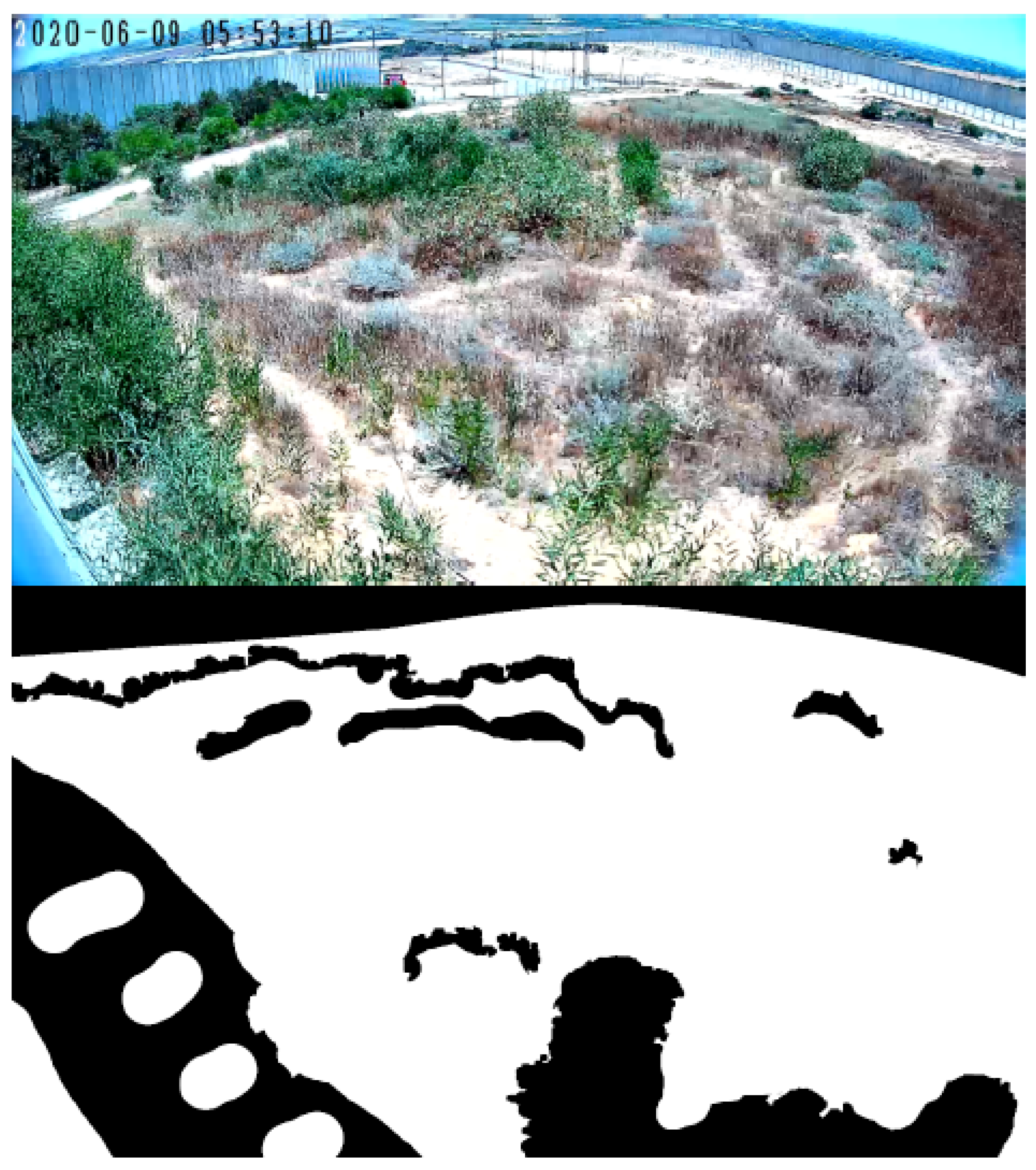
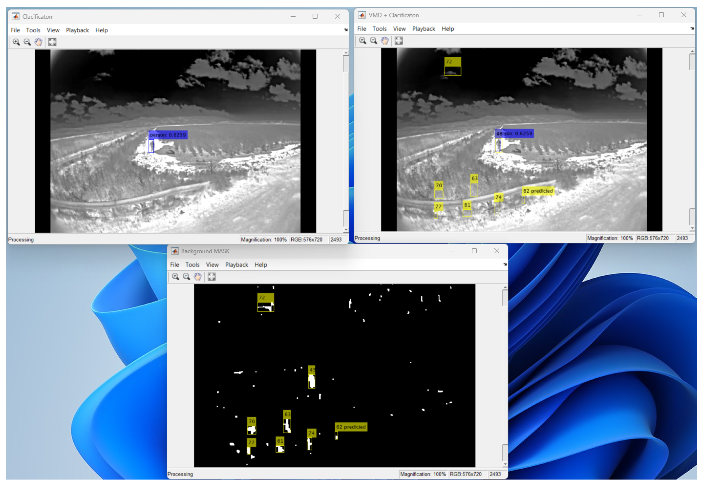
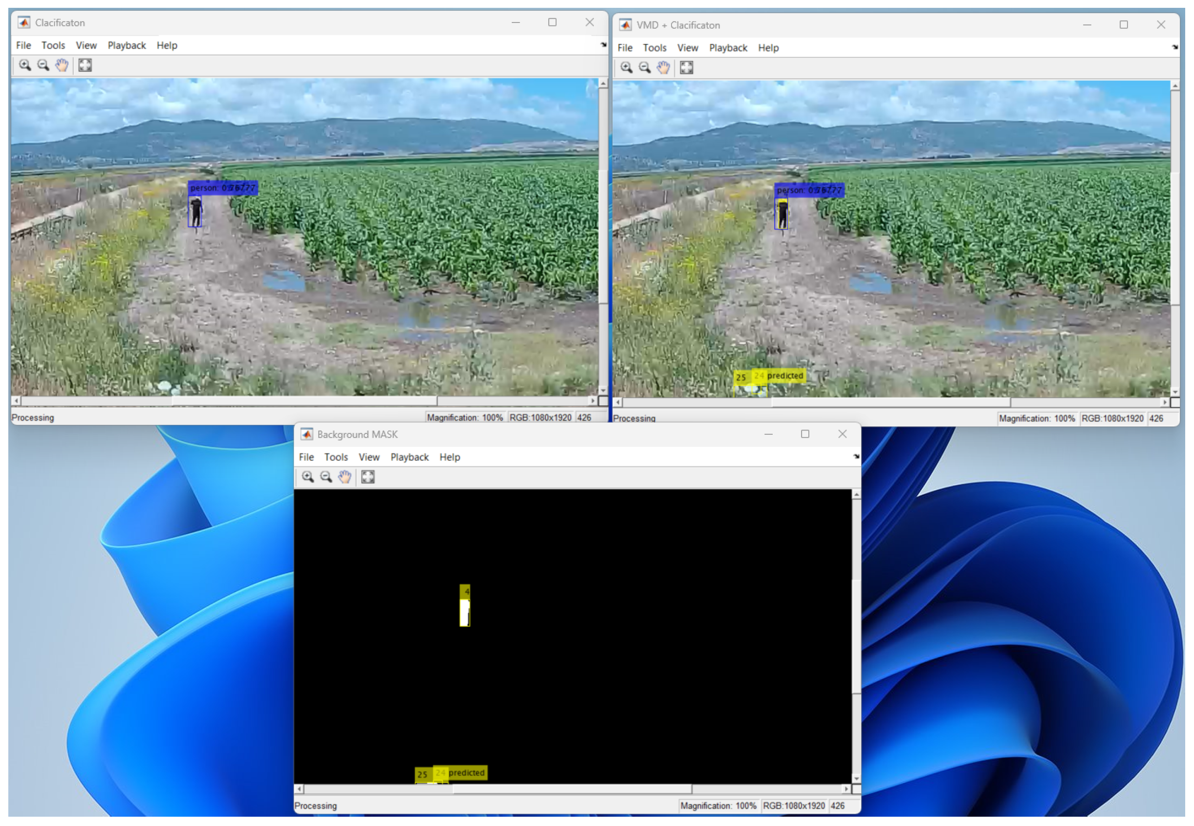
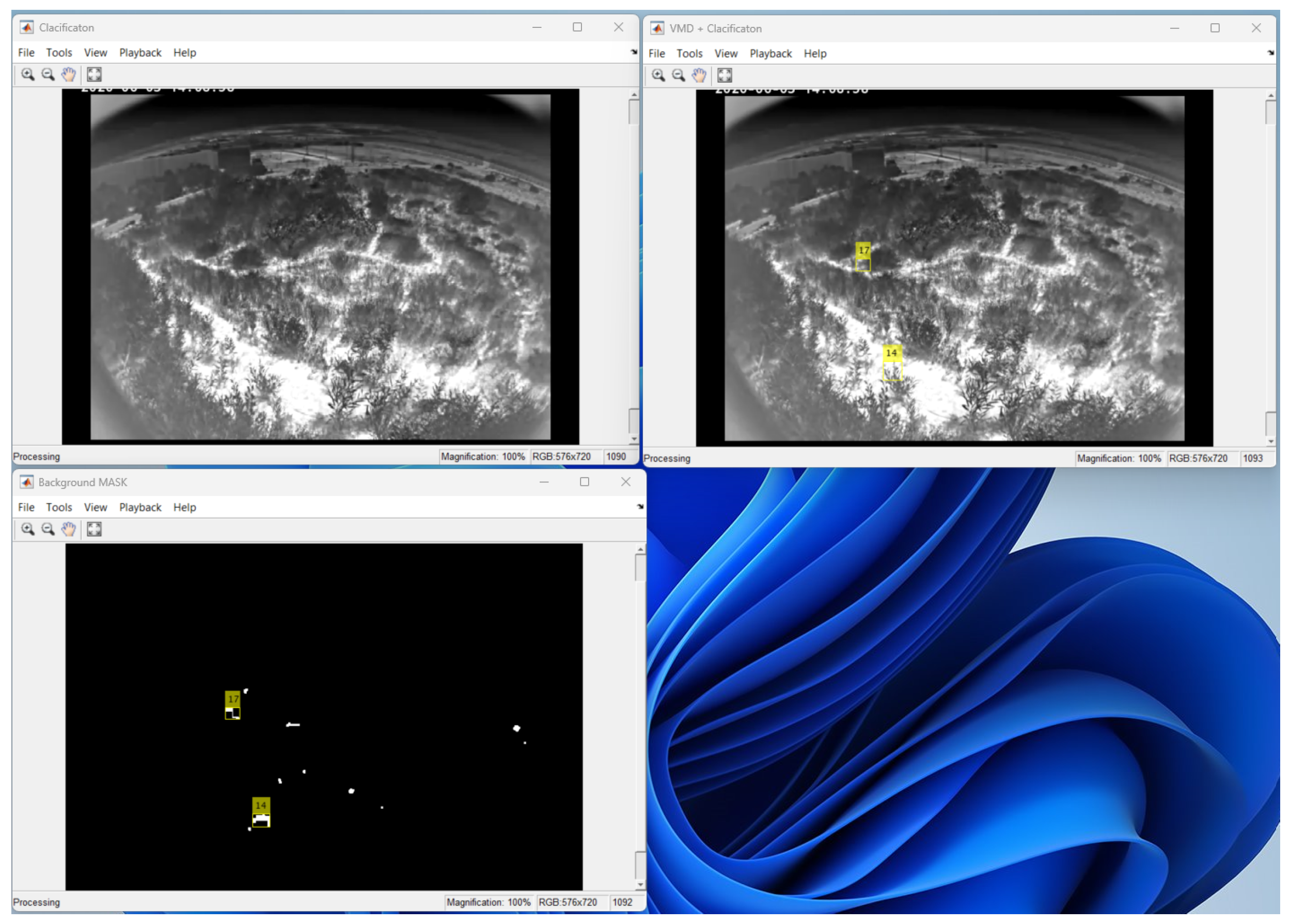
3.1.1. Background Subtraction Mask

It has been observed that the mixture of Gaussian (MOG) background subtraction model is not effective in fully distinguishing between moving background elements and foreground objects in the scene. Factors such as moving tree leaves, clouds, and sudden changes in lighting can cause significant changes in the view and can be detected as tracks. Reducing the sensitivity of the background subtraction can result in a long detection duration for distant objects as the main criteria for identifying false tracks are the duration of the track’s presence in the view and the distance traveled. This can lead to a situation where a trade-off must be made between some false detections and the undesirable long detection duration.

The background subtraction mask is a structure used to validate or discard raw detections. It is a binary mask, meaning that the detection of a specific pixel is either accepted or rejected, with no intermediate states for background–foreground segmentation. The actual implementation multiplies the background subtraction result (after a threshold has been applied) by the background subtraction mask to effectively filter the raw detections. An example of the background subtraction mask alongside a frame from a video from a test site is shown in Figure 5. The mask has zeros on regions where high-contrast moving background elements could interfere, and the sky region is fully masked as there are no relevant detections in this area.

The background subtraction mask is created through three main steps: scene variance estimation, initial background mask calculation, and mask editing. During scene variance estimation, the system runs for a set period of time (ranging from several minutes to several tens of minutes) with no objects of interest present in the scene. Images containing the minimum values $\left(Imin\right)$ and maximum values $\left(Imax\right)$ of the pixels are saved, and the total variance is calculated by taking the difference $(Imax$–$Imin)$. In the second step, a 2D low-pass filter is applied to the scene variance image, followed by a threshold operation. The output of this step is a binary image that can be used as a background subtraction mask.

One issue with using the MOG background subtraction model to generate a mask is that it does not take into account the 3D configuration of the scene or any common knowledge about the environment. There may be areas in the scene where detections are not relevant (such as the sky or high trees), but these are not considered when calculating the mask. For example, the sky may be clear during the period of variance estimation, but, during system operation, any weather conditions may be present. Clouds appearing in the sky would not be a relevant target but would still be included in the mask. Small variations in the environment due to wind, or other factors that affect the 3D configuration of the scene, can also impact the mask.

Manual mask editing allows for more precise control of the system performance based on an understanding of the underlying methods used to process the data. For example, a single high-variance background object of small size can be ignored and left in the estimation without being masked. Random, localized detections, even when the background subtraction is not perfect, can be filtered out by the tracking step. However, a series of ever-changing background objects (such as a row of bushes) can cause false tracks and false alarms. Manual mask editing allows for the removal of such objects from the mask, improving the performance of the system.

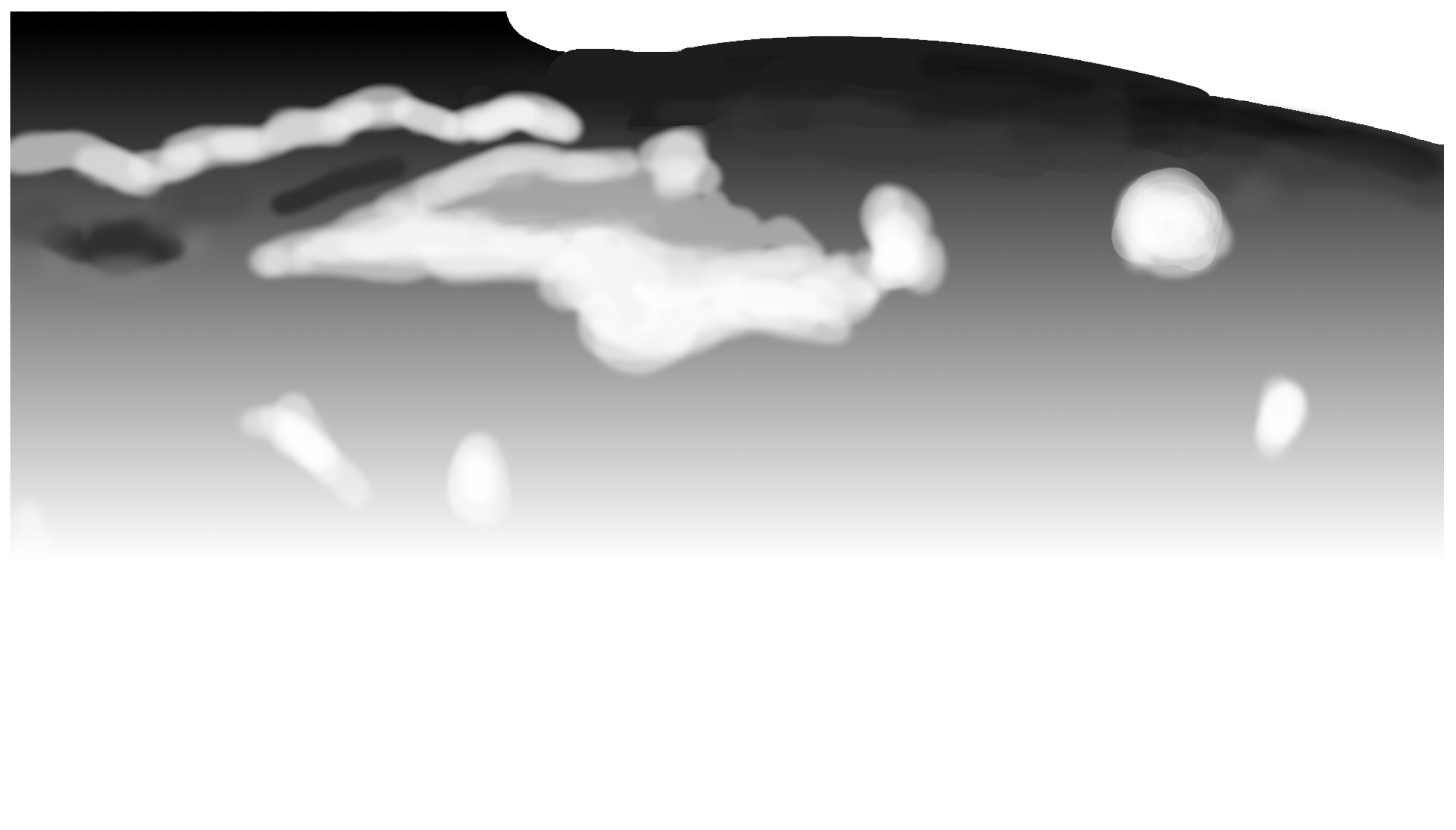
3.1.2. Parameters Scaling Mask

The parameter mask is a 2D structure similar to the background subtraction mask, representing each pixel of the video frame. It is generated using large-scale geometrical knowledge of the system setup, but is also modified manually. The main difference between the background subtraction mask and the parameters scaling mask is that the latter is a grayscale image, with pixels that can take on any value from 0 to 255. The purpose of the parameters mask is to improve the validation of potential tracks. It is applied in the tracking module, where potential tracks are validated based on various properties, such as size, duration, and distance traveled. By scaling the threshold values of these filters based on the location of the track in the scene, it is possible to have finer control over the detection probability. This can improve the overall performance of the system.

The example of the scaling mask parameters used is shown in Figure 6.

3.1.3. Fusion with a Neural Network

The track fusion scheme is a way to combine the outputs of a visual motion detection (VMD) system and a neural network (NN). In this scheme, the VMD potential tracks are compared to the NN detections based on their location in the video frame. If a VMD track matches an NN detection of the relevant class, it is considered a validated track, even if it does not meet other thresholds. The use of NN outputs allows VMD to act as more than just a motion detector. If the NN detects an object with a high score, it can be treated as a validated track right away. In the current implementation, a high score detection from the NN creates a validated VMD track by setting certain track-filtering parameters above the threshold. Further research could explore different methods for weighing the importance of score or consistency in detection between video frames.

We integrated the “You Only Look Once version 4 (YOLO v4)” object detection network with VMD detections. YOLO v4 is a one-stage object detection network composed of three main parts: the backbone, neck, and head. The backbone of YOLO v4 is typically a pre-trained convolutional neural network (CNN) like VGG16 or CSPDarkNet53, which has been trained on large datasets such as COCO or ImageNet. The backbone serves as a feature extraction network that generates feature maps from input images. The neck connects the backbone to the head. It consists of a spatial pyramid pooling (SPP) module and a path aggregation network (PAN). The SPP module combines feature maps from different layers of the backbone network, allowing for multiscale feature representation. The PAN further aggregates and processes these features for improved object detection performance. The head of YOLO v4 processes the aggregated features and generates predictions for bounding boxes, objectness scores, and classification scores. The head employs one-stage object detectors, similar to those used in YOLO v3, to perform the detection task. The YOLO v4 network is designed to achieve real-time object detection by efficiently processing images and videos. Its backbone, neck, and head work together to extract relevant features, fuse them at different stages, and produce accurate predictions for object detection. It has been established through conducted experiments that using the YOLOv4 network with its default weights is inadequate for successful object detection in certain security-related scenarios.

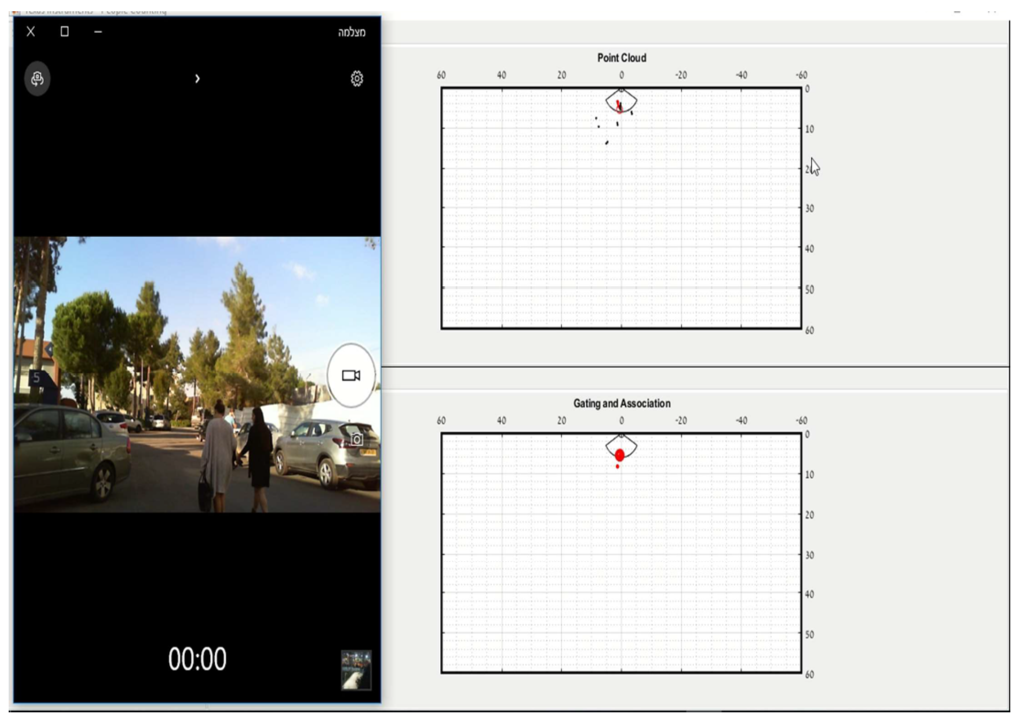
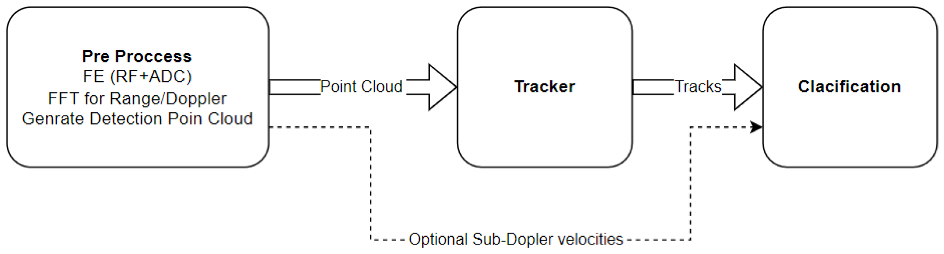
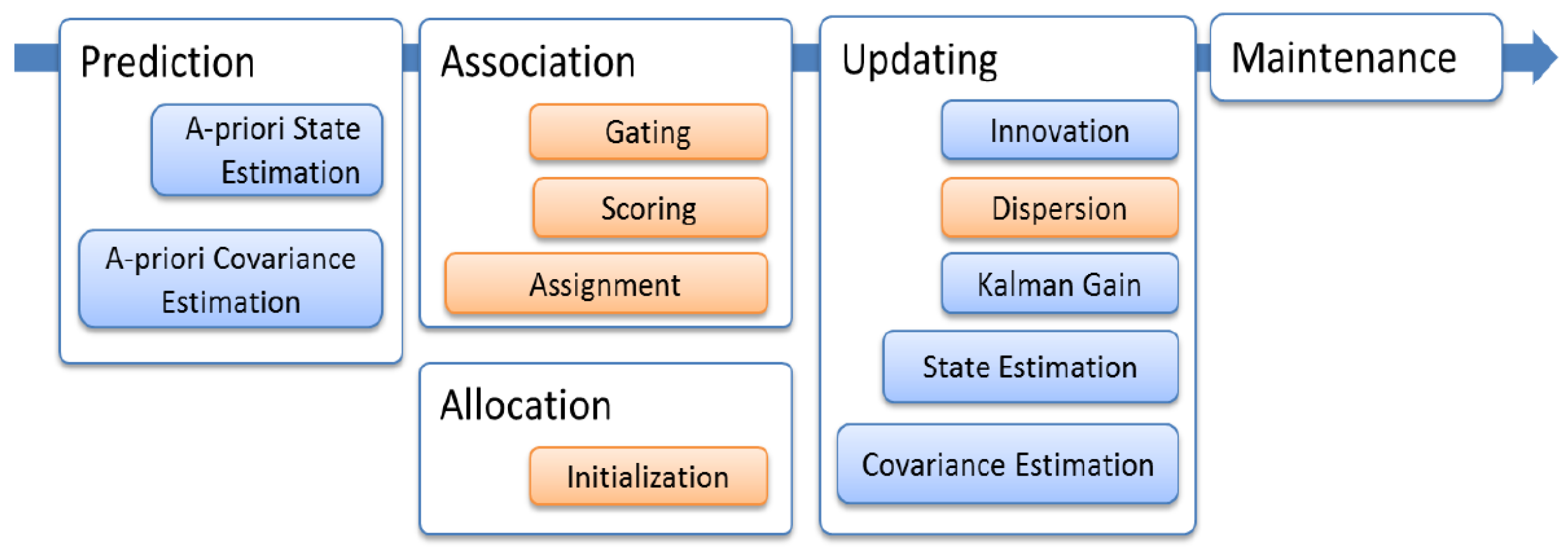
3.2. MMW Radar Object Tracking

In this section, we will discuss algorithms that were used and implemented for different setups we implemented and used for the research.

3.2.1. MMW Radar Object Tracking Used with IWR6843IS Radar

First setup is built using IWR6843IS MMW radar (Figure 7), and we will briefly review the algorithm provided by TI [60] for MMW radar object tracking and its evaluation platform. We utilized a pre-built algorithm and made adjustments to the parameters to achieve the desired performance. The tracking algorithms are integrated into the localization processing layer within the radar processing stack. The tracker collaborates with the input of the detection layer to provide localization information to the classification layers (see Figure 8). The tracking layer performs several tasks, including receiving point cloud data, conducting target localization, and delivering the results in the form of a target list to the classification layer. The tracker’s output consists of a collection of trackable objects with various properties, such as position, velocity, size, point density, and other features that can be utilized by the classifier for identification purposes. High-resolution radar sensors can detect multiple reflections from real-world targets, resulting in a substantial number of measurement vectors, collectively referred to as a point cloud. Each measurement vector represents a reflection point characterized by range, azimuth, and radial velocity and may include reliability information. These vectors are generated by the detection layer.

Due to the advantages of MMW radar in terms of accuracy, the radar target is primarily represented as multiple reflection points to the tracker layer. Groups of targets exhibit correlations in measured range, angle, and angular velocity. Multiple target scenarios are common in real-world situations, and therefore a tracker capable of handling multiple target groups is required. The group tracking approach, as depicted in Figure 9, is used to address these challenges.

The flow of the algorithm is represented in a block diagram, as shown in Figure 10, where the blue functions correspond to classical extended Kalman filter operations and the brown functions denote supplementary adjustments implemented to facilitate multi-point grouping.

3.2.2. MMW Radar Object Tracking Used with iSYS-5020 Radar

We use the implemented probabilistic data association (PDA) tracking model [61,62]. The tracking state is defined as follows:

• ID.
• State vector (range, range rate, range acceleration, azimuth, azimuth rate, azimuth acceleration).
• Timestamp (when last updated).
• Track probability.
• Age (only increased, if matching measurement is found, used as one of the properties for track validation).

The Bernoulli distribution is used to describe several aspects of the PDA (probability data association). One of those is describing the probability of positive object detection while clutter is present. If x is a detection value, which can take values 0 or 1:

$$x=\left\{\begin{array}{cc}1\hfill & \mathrm{with}\mathrm{probability}{P}^D\hfill \\ 0\hfill & \mathrm{with}\mathrm{probability}1-P^D\hfill \end{array}\right.$$

One of the main assumptions used in this document, but not necessary for PDA to be used, is that the track state update is defined as

$$x\left(k\right)=f_{k-1}x(k-1)+q_{k-1}$$

where q has a normal distribution with mean 0 and covariance $Q_{k-1}$. The probability density of the track being in state $x_k$ given the previous state $x_{k-1}$ is

$$p\left(x_k\right|x_{k-1})=\mathcal{N}(x_k;f_{k-1}\left(x_{k-1}\right);Q_{k-1})$$

which reads as the Gaussian density of $f_{k-1}\left(x_{k-1}\right)$ with covariance $Q_{k-1}$ evaluated at $x_k$.

Similarly, the probability distribution function of measurement $z_k$ given state $x_k$ (for a single target) is

$$g_k\left(z_k\right|x_k)=\mathcal{N}(z_k;h_{k-1}\left(x_k\right);R_k)$$

where $R_k$ is the covariance of normal distribution measurement noise.

It is also assumed that noise detections have a Poisson distribution (per unit of time in a given volume) with intensity ${\lambda }_c$.

Without derivation (which is explained in detail in a series of videos on single-object tracking in clutter [63] among other sources), the general formulas used for the target state (and its probability distribution function) can be summarized as follows.

The probability distribution (posterior) of the hypothesis that none of the gated detections was of the object is

$$P_{k|k}\left(x\right)=P_{k|k-1}\left(x_k\right)$$

which means it is just the prior calculated by the usual Kalman filter evaluation step.

The probability distribution (posterior) of the hypothesis that each of m gated measurements could be a real target detection is

$$P_{k|k}\left(x\right)=\mathcal{N}(x_k;{\mu }_{k|k};R_{k|k})$$

which reads as a Gaussian distribution with mean ${\mu }_{k|k}$ and covariance matrix $P_{k|k}$ evaluated at $x_k$. $P_{k|k}$ and ${\mu }_{k|k}$ are posteriors, evaluated using Kalman filter update functions while having $z^{\theta }$ (where $\theta$ takes values from 1 to m) measurements.

Weights of each hypothesis are also needed to calculate the final probability distribution of the target state given all the measurements. In the case of no measurement hypothesis:

$$w_k=w_{k-1}(1-P^D)$$

where $w_{k-1}$ is the previous time step weight, but, due to subsequent weight normalization, it can be omitted. $P^D$, as mentioned previously, is the probability of detection.

For the calculation based on one of m gated measurements:

$$w_k=P^D\frac{\mathcal{N}(z^{\theta };z_{k|k-1};S_{k|k-1})}{{\lambda }_c\left(z^{\theta }\right)}$$

where $z_{k|k-1}$ is the measurement based on prediction from $x_{k-1}$ state, $S_{k|k-1}$ is the prediction covariance. Both are calculated as per usual Kalman state update functions. ${\lambda }_c\left(z^{\theta }\right)$ is the noise intensity at measurement point $z^{\theta }$, and it may be given or calculated based on some measurement statistics.

With all probability distribution functions $P_{k|k}$ and weights $w_k$, the updated state of the target can be calculated as

$$x=\sum _{\theta }{w}_k{x}_{k|k}$$

summation here is performed over all the possible hypotheses ($\theta$ takes values from 0 to m, the index is omitted).

The updated state covariance is calculated as

$$P=\sum _{\theta }(w_k{P}_{k|k}+w_k(x-x^{\theta }){(x-x^{\theta })}^T)$$

again, summation is over $\theta$, taking values from 0 to m. The first term in the summation is called the average covariance, and the second is the spread of the mean.

Several pruning strategies can be implemented to limit processing time. For example, unverified tracks are removed if their posterior probability falls below a certain threshold. This threshold is aggressively increased when the number of tracks increases, so unverified tracks are removed from memory at a higher rate.

After calculating the updated state probability distribution function, the probability of the target being in a specific space region should be calculated as an integral in some region of state space. However, it was observed that the calculation of integrals in several dimensions for many potential tracks is not feasible. Instead, the probability of the target being in a specific state is inferred just from the maximum value of the relevant distribution. For a Gaussian distribution, the maximum is at the mean value of the distribution, and its value is inversely proportional to the covariance.

In multidimensional cases, this can be implemented as a division by the determinant of the result of the Cholesky decomposition of the covariance matrix. Finally, logarithmic probability is used:

$$p\left(x_k\right|x_{k-1},z_k)\propto log\left(\frac{1}{|\sqrt{P}|}\right)$$

or

$$p\left(x_k\right|x_{k-1},z_k)\propto -log\left(\right|\sqrt{P}\left|\right)$$

The proportionality sign is used here since all the constants involved in the calculation are removed. The full set of constants for probability calculations should be used while conducting proper integration, though. In particular, the implementation scale of relevant probabilities is built from the limits used in the model. Calculated from the above formula, $p\left(x_k\right|x_{k-1},z_k)$ can take only values from a certain range. $p_{\min }$ and $p_{\max }$ are calculated based on empirical observations of what is considered close to 100% detection probability and 0% detection probability:

$$p_{\min }=-log\left(\right|\sqrt{P_{\max }}\left|\right),p_{\max }=-log\left(\right|\sqrt{P_{\min }}\left|\right).$$

These values are calculated at initialization.

The full process of one tracking cycle:

• Update tracks by measurement.
• Merge existing tracks.
• Update clutter model.
• Create potential tracks.
• Validate tracks.

The update of the tracks is performed in two main steps: gating of candidate measurements using the Mahalanobis distance metric and updating each track. Gating is performed by first calculating the state vector and state covariance matrix priors, then calculating innovation, measurement covariance, and the Mahalanobis distance between the real measurement and the measurement that should have been observed if it had come from the evaluated state vector.

The matching of tracks is performed by calculating the distance between their state vectors (in all dimensions) but limiting the lower bound of covariances to some minimal values required by the accuracy of the track estimation. For example, the distance and angle variation fields of the covariance matrices are set to the precisions of the radar sensor even if these fields are small (precise track). Furthermore, the worst-case Mahalanobis distance between two tracks is calculated (using the smaller of the covariances). If the matching distance condition is met, attributes of tracks are merged based on policies highlighted below:

$$\begin{array}{c}\left(*\mathrm{tr}\right)!\mathrm{age}=max\left(\right(*\mathrm{tr})!\mathrm{age},(*\mathrm{tr}2)!\mathrm{age})\hfill \\ \left(*\mathrm{tr}\right)!\mathrm{ID}=min\left(\right(*\mathrm{tr})!\mathrm{ID},(*\mathrm{tr}2)!\mathrm{ID})\hfill \end{array}$$

Tracks are only selected for merging if their velocity variance is small enough, based on the idea that a track with high velocity variance is an unsettled one.

The clutter model is important for suppressing false detections and unreliable updates in regions of space where the rate of detection from stationary targets not relevant for tracking is very high. The noise intensity is calculated per state-space cell. The state-space is compressed in the dimensions of the velocities to reduce the number of calculations, so it can be described as ${\lambda }_c(r,\theta )$; i.e., it is spatial-coordinates-dependent. ${\lambda }_c$ is continuously evaluated by calculating the number of measurements that are not used to update tracks or create new tracks.

The entire scan space is split into a grid of 5 m by 5 degrees. Each detection in a given cell is added with a weight value of 1 to the current cell, and, for each neighbor (diagonal included), weight is calculated as the value of a Gaussian centered at the given cell and a predefined standard deviation. The reason is that the source of stationary detections will yield normally distributed detections in spatial dimensions.

${\lambda }_x$ values for each cell are updated using Kalman filter formulas for the state of one element:

$$\begin{array}{cc}\hfill \mathrm{num}& =(\ast it).detections;\hfill \\ \hfill (\ast it).variance& =(\ast it).variance+0.1f;//\mathrm{Process}\mathrm{noise}\hfill \\ \hfill y& =\mathrm{num}-(\ast it).lambda;//\mathrm{Innovation}\hfill \\ \hfill S& =(\ast it).variance+3.0f/(0.2f+\mathrm{num});//\mathrm{Measurement}\mathrm{noise}\hfill \\ \hfill K& =(\ast it).variance/S;//\mathrm{Kalman}\mathrm{gain}\hfill \\ \hfill (\ast it).lambda& =(\ast it).lambda+K\ast y;\hfill \\ \hfill (\ast it).variance& =(\ast it).variance-K\ast (\ast it).variance;\hfill \end{array}$$

New tracks are created from any non-stationary measurement. Before creating tracks, simple clustering of radar detections is performed: similar detections to a given one are collected, and, if there are at least 3 matches, the average of these is used to create a track.

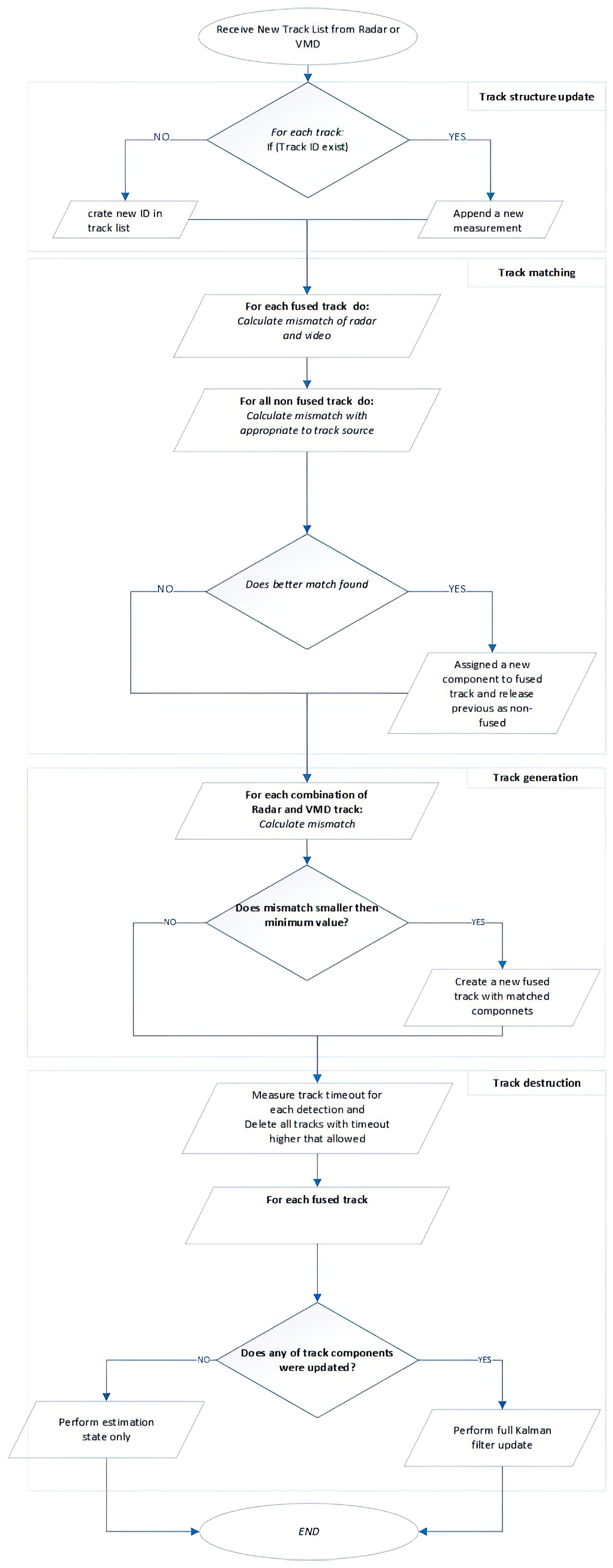
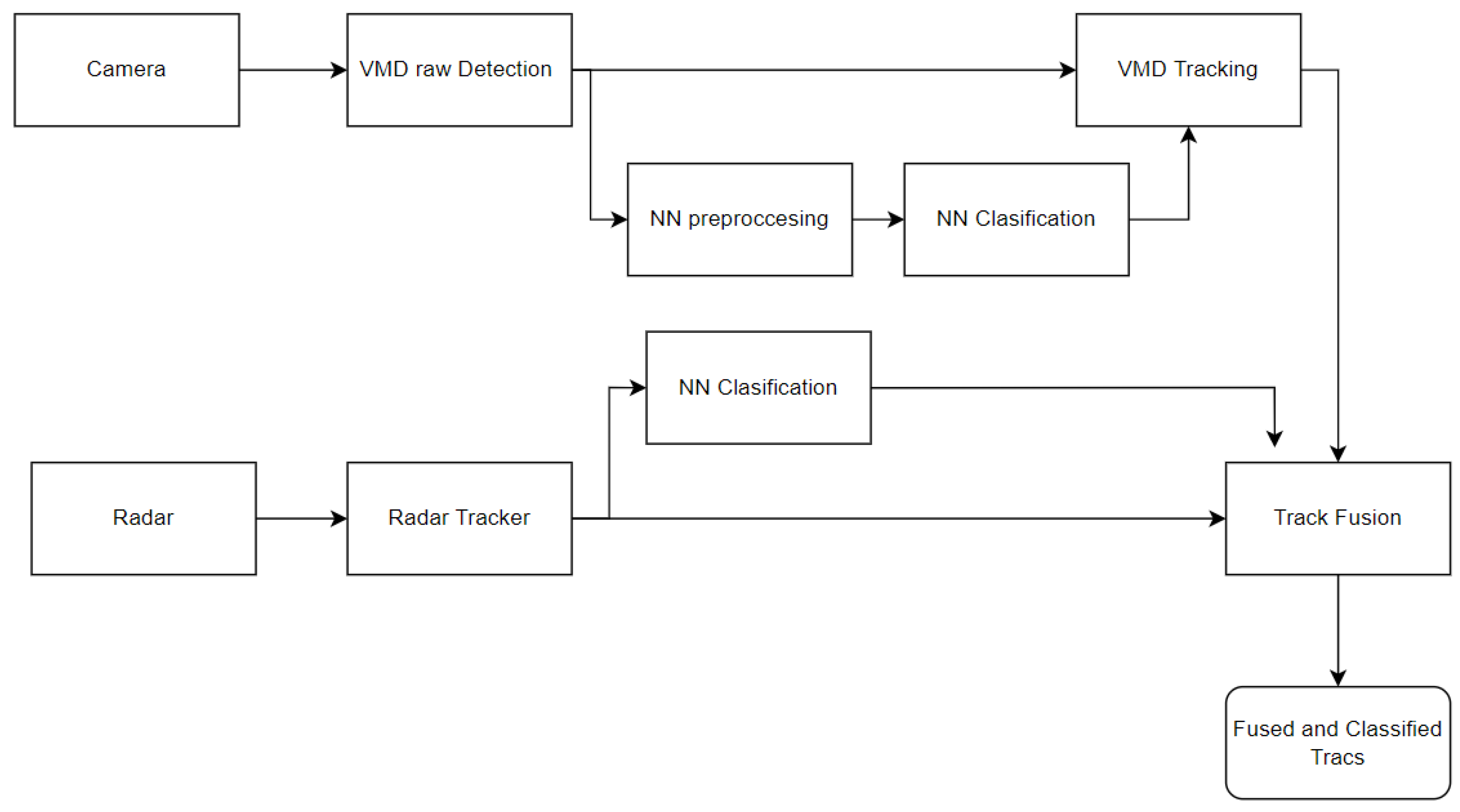
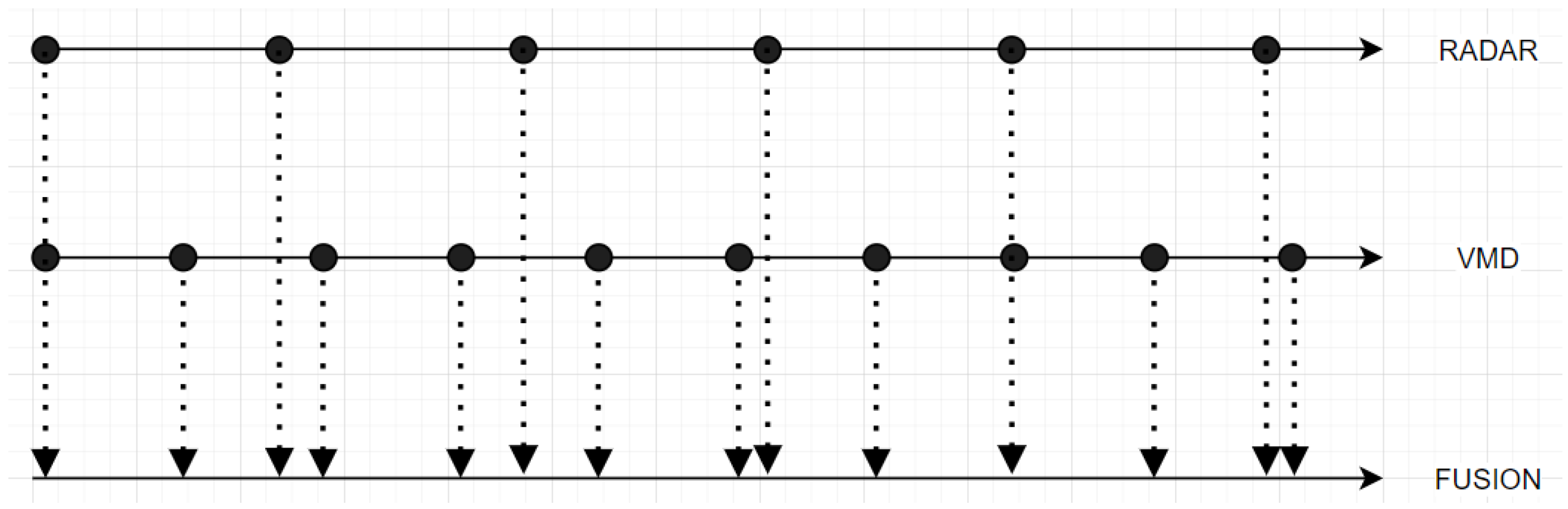
3.3. Fusion Strategy

Track Fusion

Track fusion is a distributed method to combine features (tracks) of a visual motion detection (VMD) system and a radar tracker. The fusion process is performed after the data from both sources have been processed and the tracks have been detected on both sets of data. The tracks are then matched (track-to-track association) in order to more accurately reflect the behavior of the object being tracked. If one of the sources does not return a track while the other does, different policies can be used to prioritize either reducing false detections or extending tracking duration. Track fusion is generally easier to debug and tune than data fusion because the separate modules can be tested and tuned more efficiently due to the reduced complexity of the process.

A general strategy for track fusion can be summarized as follows in Figure 11:

• It is possible for both sources (the VMD system and the radar tracker) to create fusion tracks that are not yet complete and are waiting for a match to be found at a later stage. This means that the tracks may not yet contain all the necessary information about the object being tracked, but they can still be used to help estimate the object’s location and other characteristics. Once a match is found, the fusion tracks can be updated with additional information from the other source, and the complete track will be more accurate and reliable.
• Data association (matching the tracks to the Kalman state estimate) has already been performed in the tracker, so the input tracks can be used directly in the fusion process without further verification.
• VMD and radar tracker tracks can be merged (combined) if certain requirements are met. Once the tracks are merged, the resulting fusion track will contain information from both the VMD and the radar tracker.
• The track can be split (divided) if it is determined that the visual and radar data are diverging too much. This process of track splitting and merging is performed at each step where new data is received and updates are made to the track. This allows the track to be refined and kept as accurate as possible on the basis of the most current data.

Figure 11. Track fusion algorithm.

Figure 11. Track fusion algorithm.

The track fusion algorithm involves several distinct steps. To begin, measurement timestamps are generated for all entries in both radar and moving object detection (VMD) tracks. The matching estimates are then calculated using interpolation or extrapolation techniques, as depicted in Figure 12. The average azimuth mismatch is used as a parameter for the matching, and the process may terminate prematurely if the mismatch exceeds a predefined threshold. The age of each track is updated with every new radar tracker output. Each output is treated as a new radar measurement with a time step equivalent to the duration of the radar update. If no measurements are added to a track, its timeout value is increased. The timeout value for track deletion is determined based on the current number of tracks. When the number of tracks is below the maximum track limit ($N_{\max }$), the timeout value defaults to 3 s. However, if the number of tracks exceeds $N_{\max }$, the allowed timeout value decreases. Tracks are created or initialized with each detection of moving objects from radar and each VMD detection. Upon creation, a VMD track is in a nonvalidated state, while a track created from radar tracker data starts in a validated state. If a fused track is created using both radar and VMD components, and the VMD measurements significantly deviate from the tracker output, the track can be split. In such cases, the VMD portion of the split track inherits the range data and all relevant information pertaining to the duration of detections and the track’s age. After a brief invalidation period, the VMD track can be matched again.

Algorithm 1 illustrates scoring and classification of fused tracks using the results of the classification of objects of radar and thermal camera objects.

Algorithm 1: Classification Fusion Algorithm

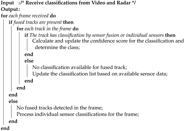
4. Experimental Results

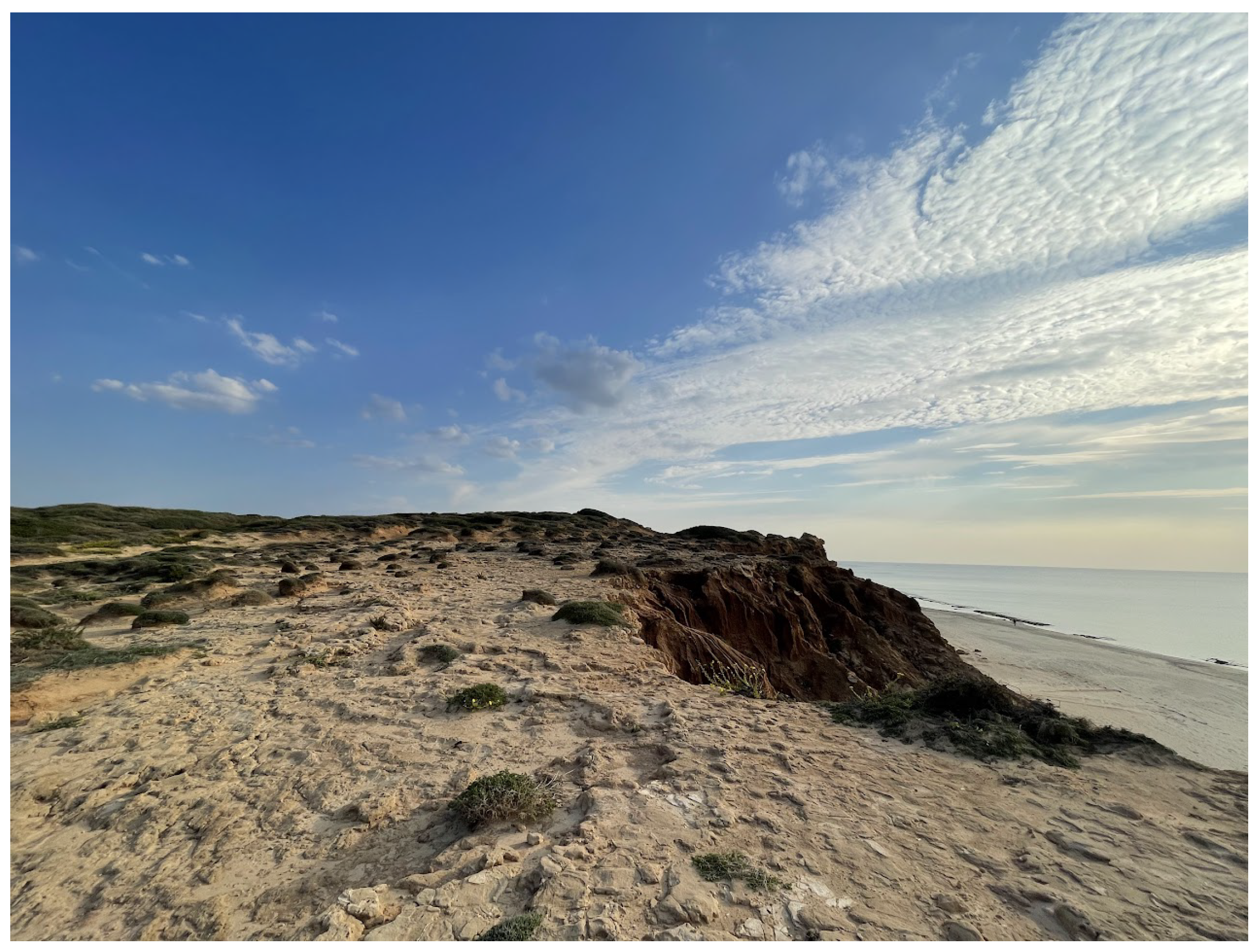
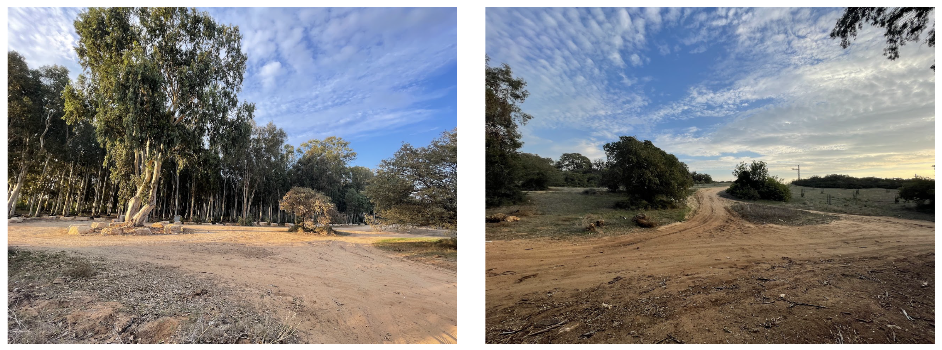
4.1. Dataset Used

The proprietary dataset used encompassed a comprehensive collection of sensor data obtained from a multisensor system designed to detect and track objects under various challenging environmental conditions in natural environments in Israel and Lithuania. This dataset includes 126 h of video information gathered from a thermal camera operating independently of lighting conditions, ensuring functionality in complete darkness. Additionally, it comprises data derived from a millimeter-wave (MMW) radar that utilizes a track-before-detection method, prioritizing the establishment of reliable object tracks before the execution of detection, gathered over a continuous period of 12 months. This particular feature proved advantageous in scenarios involving low light or smoke interference, where conventional detection methods might falter. Moreover, 12,541 object tracks were generated using a track-by-detection approach, employing Bayesian-based filters that amalgamate detections from both the thermal camera and the MMW radar, ensuring robust and accurate object tracking. The dataset was meticulously evaluated against defined criteria, including significant event detection, probability of detection, duration of detection, and false detections. Trained personnel performed diverse movement patterns (104 variants) within a 130 m range to assess the system’s performance under various operational challenges.

4.2. Metrics

Traditional metrics like the Wasserstein metric may lack a consistent physical interpretation. The scoring methods proposed by Fridling and Drummond offer a fair evaluation of multiple target tracking algorithms but may require further development of track-to-truth associations. The OSPA metric has gained popularity as the most commonly used metric for multi-target tracking [64]. It optimally assigns all targets in the test and target sets and computes the localization error based on this assignment, while also modeling cardinality mismatches with penalties. The GOSPA metric builds upon the OSPA metric by penalizing localization errors for detected, missed, and false targets in different ways. Its aim is to encourage trackers to have fewer false and missed targets. However, the improvement it provides over the original OSPA metric may be limited.

In cases where object size is also a consideration, the metric needs to be extended to include bounding-box error estimation. Conventional metrics such as MOTP and MOTA based on CLEAR metrics may not accurately describe performance when false positives occur and can be influenced by the choice of confidence threshold. The AMOTA and sAMOTA metrics have been proposed as integral and scaled accuracy metrics, respectively, to standardize the evaluation of 3D multi-object tracking [65]. However, these metrics do not consider the object size. In such cases, the OSPA metric is commonly used for tracking evaluation as it effectively balances localization error, cardinality error, and computational burden.

4.3. Test Setups

Figure 7 and Figure 13 include the image of the test setup used for the experiments.

Two test setups were built, calibrated, and tested. Test setup 1 includes IWR6843IS MMW radar (

Table 2. The main parameters of radars.

Property	Value	Value
Operating frequency	62 GHz	24 GHz
Bandwidth	1768.66 MHz	250 MHz
Chirp time	32.0 us
Range resolution	0.15 m	2 m
Speed resolution	0.4 km/h	0.5 km/h
Detection range	up to 100 m	up to 200 m
Detection speed	−50–50 km/h	−100–100 km/h
Detection angle	48 degrees (azimuth)	75 degrees (azimuth)

) from TI [66]) and Sii-Core OEM thermal camera module (

Table 3. Sii-core thermal camera parameters.

Property	Value
Sensor resolution	640 × 480
Sensor type	Uncooled Bolometr
Focal Length	FOV
35 mm	Horizontal: 17 degrees, Vertical: 13 degrees, Diagonal: 20.9 degrees
8.5 mm	Horizontal: 73 degrees, Vertical: 54 degrees, Diagonal: 93 degrees

) from Opgal [67].

Test setup 2 includes Innosent ISYS-5020 MMW radar (Table 2) [68] and Sii-Core OEM thermal camera module (Table 3).

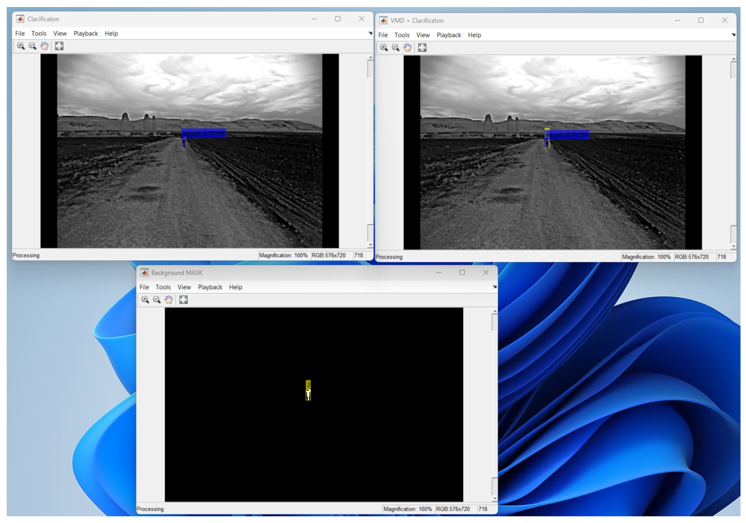
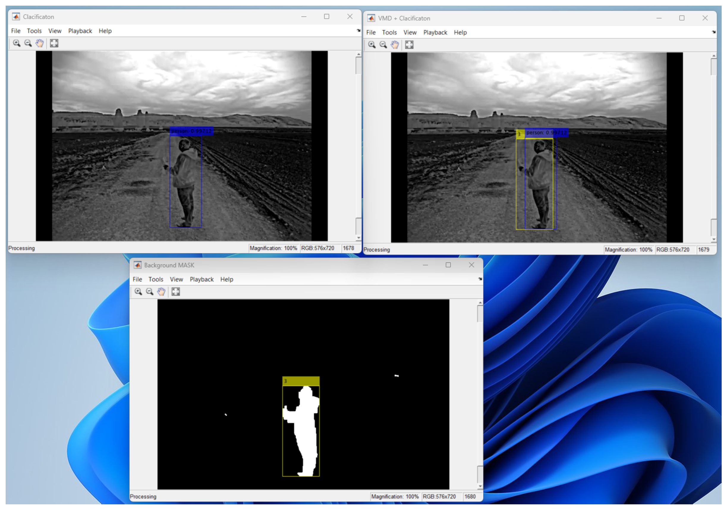
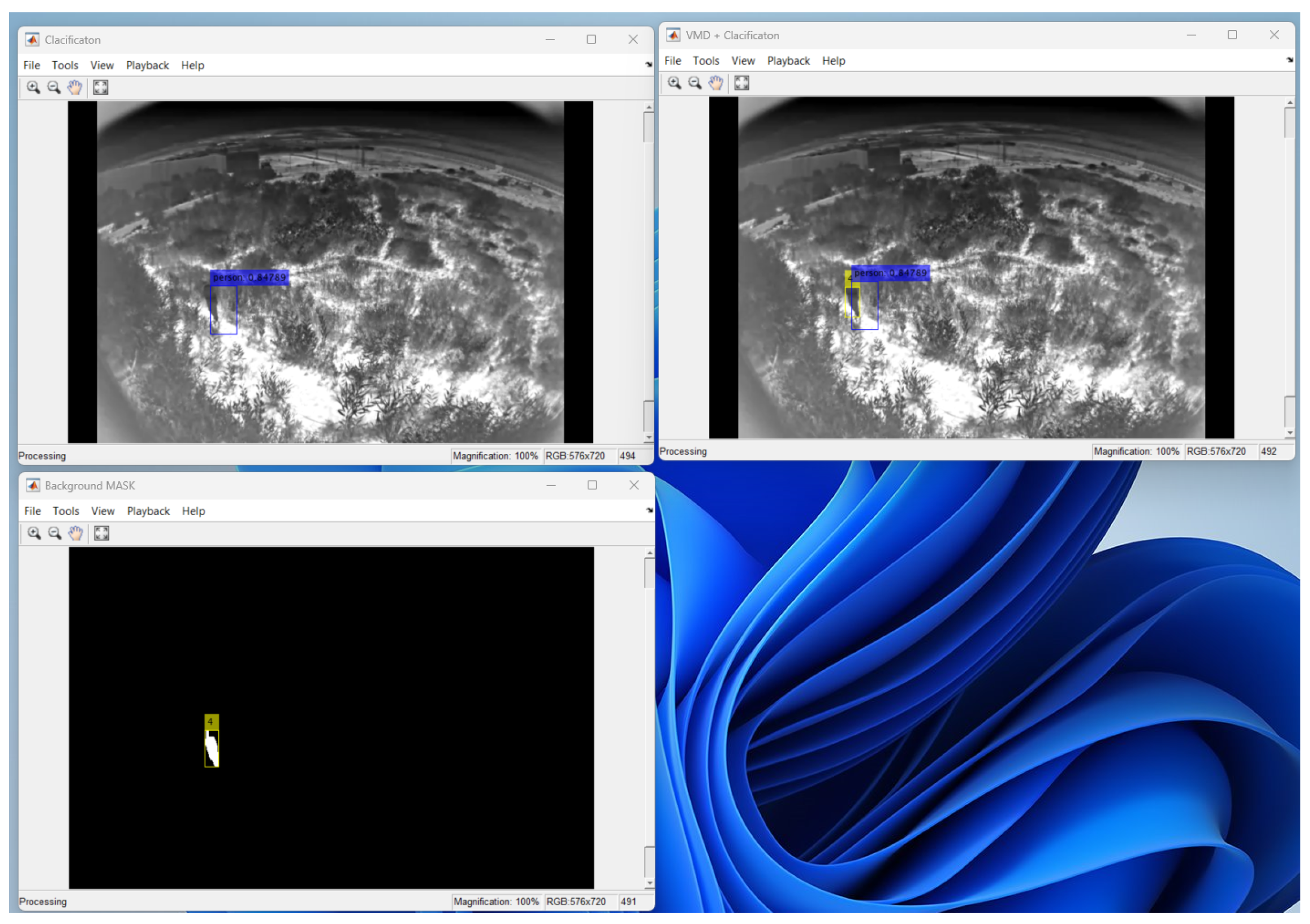
Camera Detection Test and Improvements

We conducted various tests using different scenarios to assess the effectiveness of the improvements we made to our algorithm. After each round of testing, we implemented additional algorithmic enhancements and reran the scenarios to verify their impact on performance. Throughout the research and development phase of the algorithm, we made several additions to our basic motion detection approach. We introduced a parameter scaling mask, a background addition mask, and a neural network fusion method, which helped improve the accuracy of the algorithm. By incorporating these enhancements, we were able to achieve an optimized detection level that could be fine-tuned to meet the specific performance requirements of our users. To provide a snapshot of the research angle, we have included some examples of the tests we conducted during the research and development phase of the algorithm. As you can see, the algorithm’s performance steadily improved as we introduced new features and optimizations. Ultimately, our efforts led to a highly effective and customizable motion detection system that can be customized to meet unique needs at test sites, as illustrated in Figure 14, Figure 15, Figure 16, Figure 17, Figure 18, Figure 19 and Figure 20.

Upon analysis, it became evident that fusion alone was insufficient to address the challenges regarding misdetection or oversensitivity in our detection system. Instead, we determined that, to optimize our detection capabilities, we needed to combine high accuracy with a low false alarm rate (FAR). Our goal was to develop a VMD detector that strikes the right balance between accuracy and sensitivity. We recognized the importance of being able to identify targets even if they were not classified while still minimizing the likelihood of false alarms. Therefore, we focused on improving the accuracy of our VMD detector, which would help us detect moving objects more reliably. At the same time, we worked to fine-tune the detector’s sensitivity so that it could still detect targets that were not classified without triggering false alarms. By combining these two features, we were able to achieve a highly effective detection system that strikes a balance between precision and sensitivity. This allowed us to detect moving objects with high accuracy while minimizing false alarms, ultimately leading to a more effective and reliable system.

4.4. Achieved Results

During calibration and tests, we concluded that we will be able to achieve a better result with test setup 2 in Figure 13 because the distance and angles are more suitable for the test scenarios we attempted. We wanted to achieve stable detection results for human targets for 100+ meters and could not achieve them with setup 1, although this setup has better performance with distance and speed resolution.

Table 4. Comparison of COTS tracker output and own tracker output for iSYS-5020.

	Approaching	Meeting/Crossing	Complex Enviroment
COTS tracker
Track detection distance	77.9092	58.8766	95.847
Average object count accuracy	0.817647	0.880142	0.511081
False alarm rate	0	0.0247525	0.878553
Average OSPA, (c = 1)	0.388855	0.495837	2.18644
Average OSPA, (c = 10)	1.91344	2.20029	10.6034
Average OSPA, (c = 50)	8.6894	9.69494	51.6263
Own tracker
Track detection distance	92.5097	75.8336	126.063
Average object count accuracy	0.905882	0.916934	0.900298
False alarm rate	0	0.00495049	0.108527
Average OSPA, (c = 1)	0.325851	0.363873	0.484733
Average OSPA, (c = 10)	1.1516	1.59612	2.14556
Average OSPA, (c = 50)	4.64887	6.77777	9.27821

shows the result achieved by comparing the tracer results for ISYS-5020 radar using a provider and a developed tracker.

A lack of performance for radar was observed to suffer from many missed detections only if the target trajectory was close to tangential. Another issue that was observed is that fast changes in motion direction can cause many false tracks to appear. Sensor fusion offers a solution to both problems, as shown in the evaluation results. OCA increased drastically in this case compared to radar-only tracking. It was also observed that the implemented VMD only suffers from the following limitations:

• The tracks, which are approaching and staying together, will still be merged if a single blob is reported for many frames.
• During merging/splitting of three or more objects, it is very likely that the tracks will become unstable and will often switch between objects.
• The use of velocity-based or size-based filters still requires defining the geometry of the station relative to the observed area.
• The inclusion of shadow detection, when using the mixture of Gaussians (MOG) background subtractor [69], often causes the separation of objects into two or more detections. Currently, it is not clear how to join all such detections to a single track while still being able to resolve two separate tracks moving close to one another.
• Tuning a frame memory of the MOG background subtractor does not allow to cleanly remove some periodic background movement (water, branches, etc.) while at the same time avoiding false tracks from the large-scale changes (changed lighting, slowly moving clouds).
• The detection of left/added objects cannot be performed for a long period for the same reason of large-scale changes causing many false detections.

The causes of the problems highlighted above can be separated into two large groups. Most of the issues highlighted above are caused by the fact that VMD does not recognize any single instance of objects, so several moving objects or parts of the objects are treated as a single detection. It is a fundamental problem for a detector that does not use the content of the area of interest. Related issues may be solved using recognition-based techniques. The second largest group of symptoms is caused by the fact that the number of frames used in the MOG algorithm reference frame calculation cannot be set to an optimal value. On the one hand, setting this history to some large number allows one to filter some periodic unrelated movement in the scene and allows long detection of a left object. On the other hand, a long history is not resistant to slow but large-scale changes in the scene.

In Figure 21, we present an illustrative example that shows the fusion of detection outputs from two different sources: radar and VMD (visual motion detection). Within this visualization, the radar component plays a pivotal role by not only tracing but also fusing the detected objects. This fusion process incorporates the input point cloud data obtained from the sensor, providing a comprehensive representation of the detected objects within the scene. It is also noteworthy that the forest in the background has the potential to generate false alarms, mainly due to the movement of trees. However, this challenging aspect of the environment can be effectively addressed by enhanced VMD, radar, and fusion models.

During our testing phase, we conducted a series of experiments using different scenarios for people and vehicle motion detection and measurement, in various locations. We performed over 104 different scenarios and collected data on false alarms for more than four weeks in a single location.

Table 5. Testing scenario.

Testing Scenario	Event Duration, s	Detection Duration, s	Detection Duration by Competition, s	Event Type
1	14	6	11 (7)	Person approaching
2	17	0	4 (0)	Person approaching, Was tracked from previous event
3	9	2	not detected	Person approaching and hiding
4	18	5	7 (6)	Person approaching
5	22	2.5	2 (2)	Person receding and hiding
6	9	2	not detected	Person receding from behind obstacle, Lost and retracked
7	19	2	2 (2)	Person receding and hiding
8	17	2	not detected	Car sideways, Very far
9	9	3	not detected	Person receding from behind obstacle
10	6	4	not detected	Car sideways, Was part of the background
11	18	4	not detected	Car sideways, Was part of the background
12	10	7	not detected (5)	Group approaching, Event end after the group split
13	60	2	Not detected	Car, Sideways
14	33	3	5 (5), Bus	Sideways
15	41	6	6 (6), Person	Along perimeter, partially covered
16	32	8	8 (8), Person	Along perimeter, partially covered
17	71	3.5	3 (2), Person	Receding
18	8	2	Not detected	Car, Sideways, very far
19	16	5	7 (5)	Person, Receding from previously stationary position
20	75	2	2.5 (1.5), Person	Receding, was tracked while stationary
21	35	2.5	5 (3)	Car, Sideways, very far
22	20	0	0 (0)	Person, Was tracked from previous event

presents some of the scenarios and results that were obtained. The requirements of our test sites focused on achieving low false alarm rates and high detection probability. While the client did not provide an explicit definition of the probability of detection, it was evident that the system user was more interested in the early detection of objects of interest entering the observed area.

To evaluate system performance, we defined several criteria, including important event detection (i.e., when an object of interest enters the observed area), probability of detection (i.e., the ratio of detected important events to all important events), detection duration (i.e., the average time from object appearance to detection), and false detection (i.e., movement reported by the fusion module when there was no moving object or the movement was of a non-object of interest, such as a small animal). The trained personnel performed various movement patterns, such as approaching, running, crawling, moving with stops, hiding behind an obstacle, and approaching from different distances, to evaluate footage of around 130 m. The aim was to test specific trade-offs that a system might encounter during operation.

Table 6. Average FAR and PD values for radar, VMD and fusion for complex environment.

	Radar	VMD	$\begin{array}{|c|}\hline \mathbf{Fusion}\\ \hline\end{array}$
Average object count accuracy	90%	96%	98.8%
False alarm rate (Per Day)	15	30	0.5

compares the performance of three systems—radar, VMD (video motion detection), and fusion—in a complex environment based on two key metrics: average object count accuracy and false alarm rates per day. The data reveal that, while radar achieves 90% accuracy in object counting with 15 false alarms per day, VMD outperforms it with 96% accuracy but a higher false alarm rate of 30 per day. Fusion stands out as the most accurate, achieving an object count accuracy of 98.8% while remarkably minimizing false alarms to just 0.5 per day. This comparison demonstrates that fusion excels in both accurate object counting and substantially reducing false alarms, making it an optimal choice for this complex environment.

Table 5 presents the performance results of the system for important events in the test scenarios where the algorithm did not detect false positives. We achieved a high probability of detection of 98.8%, with only a single event missed out of 104 test scenarios. In addition, we collected the false alarm rate results for two weeks of operation and examined them for each detection. The algorithm achieved the goal of detecting only three false alarms per week. Although we could have decreased the false alarm rate, it would have increased the detection time, which resulted in lower performance for short motion detections. To decrease the false alarm rate, we needed to increase the confidence for each detection. In cases where only a single source had the detection and the recognition had low confidence, we increased the time for tracking the object before reporting the detection. For short motion detections, the detection would have low performance. Overall, our results demonstrate the effectiveness of our system in achieving the desired performance parameters and provide a solid foundation for further development and improvement.

5. Conclusions and Future Works

In this paper, we present a novel approach that seamlessly integrates thermal imaging and MMW radar tracking to achieve accurate detection results while minimizing false alarms. While our approach actually provided the desired level of performance, we encountered a challenge related to the need to maintain a low false alarm rate, which led to long detection times. To address this challenge regarding detecting and identifying targets in forests and open areas, we implemented a neural network fusion module within the VMD system, complemented by a tracking-before-detection strategy applied to both the VMD and radar signals. Furthermore, we increased the confidence and probability of detection by combining the tracking data obtained from the MMW and thermal VMD radar. Additionally, we improved classification accuracy by incorporating visual classification data derived from radar tracks.

Our research efforts were primarily focused on optimizing performance, with a specific focus on achieving a high detection probability while simultaneously minimizing false alarms to as low as three false alarms per week. Although we have successfully achieved these goals and the results are impressive for stationary monitoring systems, the approach significantly increased detection duration and cannot be used for mobile or scanning platforms.

At the broader system level, our technology has the innate ability to seamlessly integrate fire detection capabilities and a diverse set of object classifications. This extends beyond security applications to encompass essential aspects of biomass monitoring. These classifications can be applied effectively to MMW radar technology, further improving our [70] detection and classification capabilities. This set of enhanced and multifaceted characteristics is of great importance, especially in the context of forest security and monitoring, where comprehensive fire detection and object classification play key roles in the preservation of our natural ecosystems.

Looking ahead, our main goal is to streamline the identification process, effectively reducing the time required while maintaining our current high levels of accuracy. We are also committed to exploring potential upgrades that will expand the versatility of our approach, making it applicable to an even wider range of use cases and scenarios. Our research lays a strong foundation for further research and development in this area and promises to significantly increase the capabilities of detection systems across a wide range of settings, including vital applications in forest security and environmental monitoring.

Sensor fusion methods still remain a key focus for future potential exploration and publication once even more meticulously curated data are obtained from operational systems installed in our national parks. We expect to provide a more extensive range of multisensor data captured in real-world scenarios, facilitating a deeper analysis of sensor fusion techniques. Future research will aim to delve into the intricacies of sensor fusion methodologies, drawing insights from the newly collected data, hopefully better and more naturally representing real-life conditions, with the anticipated goal being to seek to showcase the performance and efficacy of fusion strategies and their applications in real-life object detection and tracking.

References

1. Roman, L.A.; Conway, T.M.; Eisenman, T.S.; Koeser, A.K.; Ordóñez Barona, C.; Locke, D.H.; Jenerette, G.D.; Östberg, J.; Vogt, J. Beyond ‘trees are good’: Disservices, management costs, and tradeoffs in urban forestry. Ambio 2021, 50, 615–630. [Google Scholar] [CrossRef] [PubMed]
2. Esperon-Rodriguez, M.; Tjoelker, M.G.; Lenoir, J.; Baumgartner, J.B.; Beaumont, L.J.; Nipperess, D.A.; Power, S.A.; Richard, B.; Rymer, P.D.; Gallagher, R.V. Climate change increases global risk to urban forests. Nat. Clim. Chang. 2022, 12, 950–955. [Google Scholar] [CrossRef]
3. Keefe, R.F.; Wempe, A.M.; Becker, R.M.; Zimbelman, E.G.; Nagler, E.S.; Gilbert, S.L.; Caudill, C.C. Positioning methods and the use of location and activity data in forests. Forests 2019, 10, 458. [Google Scholar] [CrossRef] [PubMed]
4. Singh, R.; Gehlot, A.; Akram, S.V.; Thakur, A.K.; Buddhi, D.; Das, P.K. Forest 4.0: Digitalization of forest using the Internet of Things (IoT). J. King Saud. Univ. Comput. Inf. Sci. 2022, 34, 5587–5601. [Google Scholar] [CrossRef]
5. Borges, P.; Peynot, T.; Liang, S.; Arain, B.; Wildie, M.; Minareci, M.; Lichman, S.; Samvedi, G.; Sa, I.; Hudson, N.; et al. A survey on terrain traversability analysis for autonomous ground vehicles: Methods, sensors, and challenges. Field Robot. 2022, 2, 1567–1627. [Google Scholar] [CrossRef]
6. Blasch, E.; Pham, T.; Chong, C.Y.; Koch, W.; Leung, H.; Braines, D.; Abdelzaher, T. Machine learning/artificial intelligence for sensor data fusion–opportunities and challenges. IEEE Aerosp. Electron. Syst. Mag. 2021, 36, 80–93. [Google Scholar] [CrossRef]
7. Fayyad, J.; Jaradat, M.A.; Gruyer, D.; Najjaran, H. Deep learning sensor fusion for autonomous vehicle perception and localization: A review. Sensors 2020, 20, 4220. [Google Scholar] [CrossRef]
8. Ma, K.; Zhang, H.; Wang, R.; Zhang, Z. Target tracking system for multi-sensor data fusion. In Proceedings of the 2017 IEEE 2nd Information Technology, Networking, Electronic and Automation Control Conference (ITNEC), Chengdu, China, 15–17 December 2017; pp. 1768–1772. [Google Scholar]
9. Guimarães, N.; Pádua, L.; Marques, P.; Silva, N.; Peres, E.; Sousa, J.J. Forestry remote sensing from unmanned aerial vehicles: A review focusing on the data, processing and potentialities. Remote. Sens. 2020, 12, 1046. [Google Scholar] [CrossRef]
10. Qiu, S.; Zhao, H.; Jiang, N.; Wang, Z.; Liu, L.; An, Y.; Zhao, H.; Miao, X.; Liu, R.; Fortino, G. Multi-sensor information fusion based on machine learning for real applications in human activity recognition: State-of-the-art and research challenges. Inf. Fusion 2022, 80, 241–265. [Google Scholar] [CrossRef]
11. Rizi, M.H.P.; Seno, S.A.H. A systematic review of technologies and solutions to improve security and privacy protection of citizens in the smart city. Internet Things 2022, 20, 100584. [Google Scholar] [CrossRef]
12. Elmustafa, S.A.A.; Mujtaba, E.Y. Internet of things in smart environment: Concept, applications, challenges, and future directions. World Sci. News 2019, 134, 1–51. [Google Scholar]
13. Nobis, F.; Geisslinger, M.; Weber, M.; Betz, J.; Lienkamp, M. A deep learning-based radar and camera sensor fusion architecture for object detection. In 2019 Sensor Data Fusion: Trends, Solutions, Applications (SDF); IEEE: Piscataway, NJ, USA, 2019; pp. 1–7. [Google Scholar]
14. Vo, B.N.; Mallick, M.; Bar-Shalom, Y.; Coraluppi, S.; Osborne, R.; Mahler, R.; Vo, B.T. Multitarget tracking. In Wiley Encyclopedia of Electrical and Electronics Engineering; John Wiley & Sons, Inc.: Hoboken, NJ, USA, 2015. [Google Scholar]
15. Zhu, Y.; Wang, T.; Zhu, S. Adaptive Multi-Pedestrian Tracking by Multi-Sensor: Track-to-Track Fusion Using Monocular 3D Detection and MMW Radar. Remote Sens. 2022, 14, 1837. [Google Scholar] [CrossRef]
16. Tan, M.; Chao, W.; Cheng, J.K.; Zhou, M.; Ma, Y.; Jiang, X.; Ge, J.; Yu, L.; Feng, L. Animal detection and classification from camera trap images using different mainstream object detection architectures. Animals 2022, 12, 1976. [Google Scholar] [CrossRef] [PubMed]
17. Feichtenhofer, C.; Pin, A.; Zisserman, A. Detect to Track and Track to Detect. In Proceedings of the IEEE International Conference on Computer Vision, Venice, Italy, 22–29 October 2017. [Google Scholar] [CrossRef]
18. Andriluka, M.; Roth, S.; Schiele, B. People-tracking-by-detection and people-detection-by-tracking. In Proceedings of the IEEE Conference on Computer Vision and Pattern Recognition, Anchorage, AK, USA, 23–28 June 2008; Volume 14. [Google Scholar] [CrossRef]
19. Zvonko, R. A study of a target tracking method using Global Nearest Neighbor algorithm. Vojnoteh. Glas. 2006, 54, 160–167. [Google Scholar]
20. Thomas, F.; Bar-Shalom, Y.; Scheffe, M. Sonar tracking of multiple targets using joint probabilistic data association. IEEE J. Ocean. Eng. 1983, 8, 173–184. [Google Scholar] [CrossRef]
21. Reid, D. An algorithm for tracking multiple targets. IEEE Trans. Autom. Control. 1979, 24, 843–854. [Google Scholar] [CrossRef]
22. Kalman, R.E. A New Approach to Linear Filtering and Prediction Problems. J. Basic Eng. 1960, 82, 35–45. [Google Scholar] [CrossRef]
23. Simon, J.; Julier, J.K.U. New extension of the Kalman filter to nonlinear systems. Signal Process. Sens. Fusion Target Recognit. VI 1997, 3068, 182–193. [Google Scholar]
24. Welch, G.; Bishop, G. An Introduction to the Kalman Filter; Department of Computer Science, University of North Carolina: Chapel Hill, NC, USA, 1999. [Google Scholar]
25. Blackman, S.S.; Popoli, R. Design and Analysis of Modern Tracking Systems; Artech House: Norwood, MA, USA, 1999. [Google Scholar]
26. Blackman, S. Multiple hypothesis tracking for multiple target tracking. IEEE Trans. Aerosp. Electron. Syst. 2004, 19, 5–18. [Google Scholar] [CrossRef]
27. Mahler, R. Multitarget Bayes Filtering via First-Order Multitarget Moments. IEEE Trans. Aerosp. Electron. Syst. 2003, 39, 1152–1178. [Google Scholar] [CrossRef]
28. Lahoz-Monfort, J.J.; Magrath, M.J. A comprehensive overview of technologies for species and habitat monitoring and conservation. BioScience 2021, 71, 1038–1062. [Google Scholar] [CrossRef] [PubMed]
29. Yang, J.; Wang, C.; Jiang, B.; Song, H.; Meng, Q. Visual perception enabled industry intelligence: State of the art, challenges and prospects. IEEE Trans. Ind. Inform. 2020, 17, 2204–2219. [Google Scholar] [CrossRef]
30. Adaval, R.; Saluja, G.; Jiang, Y. Seeing and thinking in pictures: A review of visual information processing. Consum. Psychol. Rev. 2019, 2, 50–69. [Google Scholar] [CrossRef]
31. Kahmen, O.; Rofallski, R.; Luhmann, T. Impact of stereo camera calibration to object accuracy in multimedia photogrammetry. Remote. Sens. 2020, 12, 2057. [Google Scholar] [CrossRef]
32. Garg, R.; Wadhwa, N.; Ansari, S.; Barron, J.T. Learning single camera depth estimation using dual-pixels. In Proceedings of the IEEE/CVF International Conference on Computer Vision, Seoul, Republic of Korea, 2 October–2 November 2019; pp. 7628–7637. [Google Scholar]
33. Hu, J.; Zhang, Y.; Okatani, T. Visualization of convolutional neural networks for monocular depth estimation. In Proceedings of the IEEE/CVF International Conference on Computer Vision, Seoul, Republic of Korea, 2 October–2 November 2019; pp. 3869–3878. [Google Scholar]
34. Arnold, E.; Al-Jarrah, O.Y.; Dianati, M.; Fallah, S.; Oxtoby, D.; Mouzakitis, A. A Survey on 3D Object Detection Methods for Autonomous Driving Applications. IEEE Trans. Intell. Transp. Syst. 2019, 20, 3782–3795. [Google Scholar] [CrossRef]
35. Qian, R.; Lai, X.L.X. 3D Object Detection for Autonomous Driving. A Survey. Pattern Recognit. 2021, 39, 1152–1178. [Google Scholar] [CrossRef]
36. Zhang, Y.; Carballo, A.; Yang, H.; Takeda, K. Perception and sensing for autonomous vehicles under adverse weather conditions: A survey. ISPRS J. Photogramm. Remote. Sens. 2023, 196, 146–177. [Google Scholar] [CrossRef]
37. Jha, U.S. The millimeter Wave (mmW) radar characterization, testing, verification challenges and opportunities. In Proceedings of the 2018 IEEE Autotestcon, National Harbor, MD, USA, 17–20 September 2018; pp. 1–5. [Google Scholar]
38. Katkevičius, A.; Plonis, D.; Damaševičius, R.; Maskeliūnas, R. Trends of microwave devices design based on artificial neural networks: A review. Electronics 2022, 11, 2360. [Google Scholar] [CrossRef]
39. Plonis, D.; Katkevičius, A.; Gurskas, A.; Urbanavičius, V.; Maskeliūnas, R.; Damaševičius, R. Prediction of meander delay system parameters for internet-of-things devices using pareto-optimal artificial neural network and multiple linear regression. IEEE Access 2020, 8, 39525–39535. [Google Scholar] [CrossRef]
40. van Berlo, B.; Elkelany, A.; Ozcelebi, T.; Meratnia, N. Millimeter Wave Sensing: A Review of Application Pipelines and Building Blocks. IEEE Sens. J. 2021, 8, 10332–10368. [Google Scholar] [CrossRef]
41. Hurl, B.; Czarnecki, K.; Waslander, S. Precise synthetic image and lidar (presil) dataset for autonomous vehicle perception. In Proceedings of the 2019 IEEE Intelligent Vehicles Symposium (IV), Paris, France, 9–12 June 2019; pp. 2522–2529. [Google Scholar]
42. Ilci, V.; Toth, C. High definition 3D map creation using GNSS/IMU/LiDAR sensor integration to support autonomous vehicle navigation. Sensors 2020, 20, 899. [Google Scholar] [CrossRef] [PubMed]
43. Raj, T.; Hanim Hashim, F.; Baseri Huddin, A.; Ibrahim, M.F.; Hussain, A. A survey on LiDAR scanning mechanisms. Electronics 2020, 9, 741. [Google Scholar] [CrossRef]
44. Wang, Z.; Wu, Y.; Niu, Q. Multi-Sensor Fusion in Automated Driving: A Survey. IEEE Sens. J. 2019, 21, 2847–2868. [Google Scholar] [CrossRef]
45. Buchman, D.; Drozdov, M.; Mackute-Varoneckiene, A.; Krilavicius, T. Visual and Radar Sensor Fusion for Perimeter Protection and Homeland Security on Edge. In Proceedings of the IVUS 2020: Information Society and University Studies, Kaunas, Lithuania, 23 April 2020; Volume 21. [Google Scholar]
46. Zhao, X.; Sun, P.; Xu, Z.; Min, H.; Yu, H. Fusion of 3D LIDAR and Camera Data for Object Detection in Autonomous Vehicle Applications. IEEE Sens. J. 2020, 20, 4901–4913. [Google Scholar] [CrossRef]
47. Samal, K.; Kumawat, H.; Saha, P.; Wolf, M.; Mukhopadhyay, S. Task-Driven RGB-Lidar Fusion for Object Tracking in Resource-Efficient Autonomous System. In Proceedings of the IVUS 2020: Information Society and University Studies, Kaunas, Lithuania, 23 April 2020; Volume 7, pp. 102–112. [Google Scholar]
48. Varone, G.; Boulila, W.; Driss, M.; Kumari, S.; Khan, M.K.; Gadekallu, T.R.; Hussain, A. Finger pinching and imagination classification: A fusion of CNN architectures for IoMT-enabled BCI applications. Inf. Fusion 2024, 101, 102006. [Google Scholar] [CrossRef]
49. Lee, K.H.; Kanzawa, Y.; Derry, M.; James, M.R. Multi-Target Track-to-Track Fusion Based on Permutation Matrix Track Association. In Proceedings of the 2018 IEEE Intelligent Vehicles Symposium (IV), Changshu, China, 26–30 June 2018. [Google Scholar]
50. Kong, L.; Peng, X.; Chen, Y.; Wang, P.; Xu, M. Multi-sensor measurement and data fusion technology for manufacturing process monitoring: A literature review. Int. J. Extrem. Manuf. 2020, 2, 022001. [Google Scholar] [CrossRef]
51. Nweke, H.F.; Teh, Y.W.; Mujtaba, G.; Al-Garadi, M.A. Data fusion and multiple classifier systems for human activity detection and health monitoring: Review and open research directions. Inf. Fusion 2019, 46, 147–170. [Google Scholar] [CrossRef]
52. El Madawi, K.; Rashed, H.; El Sallab, A.; Nasr, O.; Kamel, H.; Yogamani, S. Rgb and lidar fusion based 3d semantic segmentation for autonomous driving. In Proceedings of the 2019 IEEE Intelligent Transportation Systems Conference (ITSC), Auckland, New Zealand, 27–30 October 2019; pp. 7–12. [Google Scholar]
53. Qi, R.N.H. CenterFusion: Center-based Radar and Camera Fusion for 3D Object Detection. In Proceedings of the 2021 IEEE Winter Conference on Applications of Computer Vision (WACV), Virtual, 5–9 January 2021. [Google Scholar]
54. Wang, X.; Xu, L.; Sun, H.; Xin, J.; Zheng, N. On-Road Vehicle Detection and Tracking Using MMW Radar and Monovision Fusion. IEEE Trans. Intell. Transp. Syst. 2016, 17, 2075–2084. [Google Scholar] [CrossRef]
55. Chang, S.; Zhang, Y.; Zhang, F.; Zhao, X.; Huang, S.; Feng, Z.; Wei, Z. Spatial Attention Fusion for Obstacle Detection Using MmWave Radar and Vision Sensor. Sensors 2020, 20, 956. [Google Scholar] [CrossRef]
56. Zhang, W.; Zhou, H.; Sun, S.; Wang, Z.; Shi, J.; Loy, C.C. Robust Multi-Modality Multi-Object Tracking. In Proceedings of the 2019 IEEE/CVF International Conference on Computer Vision (ICCV), Seoul, Republic of Korea, 27 October–2 November 2020. [Google Scholar]
57. Wang, Z.; Miao, X.; Huang, Z.; Luo, H. Research of Target Detection and Classification Techniques Using Millimeter-Wave Radar and Vision Sensors. Remote Sens. 2021, 13, 1064. [Google Scholar] [CrossRef]
58. Cao, R.Z.S. Extending Reliability of mmWave Radar Tracking and Detection via Fusion With Camera. IEEE Access 2021, 7, 137065–137079. [Google Scholar]
59. Kim, H.S.W.C.H. Robust Vision-Based Relative-Localization Approach Using an RGB-Depth Camera and LiDAR Sensor Fusion. IEEE Trans. Ind. Electron. 2016, 63, 3725–3736. [Google Scholar]
60. Texas Instruments. Tracking Radar Targets with Multiple Reflection Points; Texas Instruments: Dallas, TX, USA, 2018; Available online: https://dev.ti.com/tirex/explore/content/mmwave_industrial_toolbox_3_2_0/labs/lab0013_traffic_monitoring_16xx/src/mss/gtrack/docs/Tracking_radar_targets_with_multiple_reflection_points.pdf (accessed on 2 October 2023).
61. Kirubarajan, T.; Bar-Shalom, Y.; Blair, W.D.; Watson, G.A. IMMPDA solution to benchmark for radar resource allocation and tracking in the presence of ECM. IEEE Trans. Aerosp. Electron. Syst. 1998, 34, 1023–1036. [Google Scholar] [CrossRef]
62. Otto, C.; Gerber, W.; León, F.P.; Wirnitzer, J. A Joint Integrated Probabilistic Data Association Filter for pedestrian tracking across blind regions using monocular camera and radar. In Proceedings of the 2012 IEEE Intelligent Vehicles Symposium, Alcala de Henares, Spain, 3–7 June 2012. [Google Scholar]
63. Svensson, L.; Granström, K. Multiple Object Tracking. Available online: https://www.youtube.com/channel/UCa2-fpj6AV8T6JK1uTRuFpw (accessed on 15 October 2019).
64. Shi, X.; Yang, F.; Tong, F.; Lian, H. A comprehensive performance metric for evaluation of multi-target tracking algorithms. In Proceedings of the 2017 3rd International Conference on Information Management (ICIM), Chengdu, China, 21–23 April 2017; pp. 373–377. [Google Scholar]
65. Weng, X.; Wang, J.; Held, D.; Kitani, K. 3d multi-object tracking: A baseline and new evaluation metrics. In Proceedings of the 2020 IEEE/RSJ International Conference on Intelligent Robots and Systems (IROS), Las Vegas, NV, USA, 25–29 October 2020; pp. 10359–10366. [Google Scholar]
66. Texas Instruments. IWR6843ISK. Available online: https://www.ti.com.cn/tool/IWR6843ISK (accessed on 2 October 2023).
67. Opgal. 2023. Available online: https://www.opgal.com/products/sii-uc-uncooled-thermal-core/ (accessed on 2 October 2023).
68. iSYS-5020 Radarsystem for Security Applications. Available online: https://www.innosent.de/en/radar-systems/isys-5020-radar-system/ (accessed on 2 October 2023).
69. pen Source Computer Vision. cv::BackgroundSubtractorMOG2 Class Reference. Available online: https://docs.opencv.org/4.1.0/d7/d7b/classcv_1_1BackgroundSubtractorMOG2.html (accessed on 2 October 2023).
70. Buchman, D.; Drozdov, M.; Krilavičius, T.; Maskeliūnas, R.; Damaševičius, R. Pedestrian and Animal Recognition Using Doppler Radar Signature and Deep Learning. Sensors 2022, 22, 3456. [Google Scholar] [CrossRef]
71. Liu, Q.; Li, X.; He, Z.; Li, C.; Li, J.; Zhou, Z.; Yuan, D.; Li, J.; Yang, K.; Fan, N.; et al. LSOTB-TIR: A Large-Scale High-Diversity Thermal Infrared Object Tracking Benchmark. In Proceedings of the 28th ACM International Conference on Multimedia (MM ’20), Seattle, WA, USA, 12–16 October 2020. [Google Scholar] [CrossRef]
72. Banuls, A.; Mandow, A.; Vázquez-Martín, R.; Morales, J.; García-Cerezo, A. Object Detection from Thermal Infrared and Visible Light Cameras in Search and Rescue Scenes. In Proceedings of the 2020 IEEE International Symposium on Safety, Security, and Rescue Robotics (SSRR) 2020, Abu Dhabi, United Arab Emirates, 4–6 November 2020. [Google Scholar] [CrossRef]
73. Haseeb, M.A.; Ristić-Durrant, D.; Gräser, A. Long-range obstacle detection from a monocular camera. In Proceedings of the 9th International Conference on Circuits, Systems, Control, Signals (CSCS18), Sliema, Malta, 22–24 June 2018. [Google Scholar]
74. Huang, K.C.; Wu, T.H.; Su, H.T.; Hsu, W.H. MonoDTR: Monocular 3D Object Detection with Depth-Aware Transformer. In Proceedings of the CVPR, New Orleans, LA, USA, 19–24 June 2022. [Google Scholar]
75. Texas Instruments. Tracking Radar Targets with Multiple Reflection Points; Texas Instruments: Dallas, TX, USA, 2021; Available online: https://dev.ti.com/tirex/explore/node?node=A__AAylBLCUuYnsMFERA.sL8g__com.ti.mmwave_industrial_toolbox__VLyFKFf__LATEST (accessed on 2 October 2023).
Figure 1. Gador Nature Reserve; coordinates: [32.424939, 34.873738].
Forests 14 02335 g001
Figure 2. Hadera planted forest (old plantation on right and new one on left image); coordinates: [32.417927, 34.890286].
Forests 14 02335 g002
Figure 3. Algorithm flow diagram.
Forests 14 02335 g003
Figure 4. Visual motion detection and tracking flow diagram.
Forests 14 02335 g004
Figure 5. An example of the background subtraction mask (top) used for the video (bottom) while processing in VMD.
Forests 14 02335 g005
Figure 6. An example of the parameters scaling mask.
Forests 14 02335 g006
Figure 7. Test setup with 62 GHz radar.
Forests 14 02335 g007
Figure 8. Radar processing layers.
Forests 14 02335 g008
Figure 9. Group tracking.
Forests 14 02335 g009
Figure 10. Radar tracking block diagram.
Forests 14 02335 g010
Figure 12. Time alignment of radar and VMD tracks for matching.
Forests 14 02335 g012
Figure 13. Test setup with 24 Ghz radar.
Forests 14 02335 g013
Figure 14. Fused tests scene 1.
Forests 14 02335 g014
Figure 15. Fused tests scene 2.
Forests 14 02335 g015
Figure 16. Fused tests scene 3.
Forests 14 02335 g016
Figure 17. Fused tests scene 4.
Forests 14 02335 g017
Figure 18. Fused tests scene 5—thermal camera.
Forests 14 02335 g018
Figure 19. Fused tests scene 5—day camera.
Forests 14 02335 g019
Figure 20. Pure VMD faulty detections.
Forests 14 02335 g020
Figure 21. Fused tests scene 6—day camera + radar.
Forests 14 02335 g021