Research on Tree Pith Location in Radial Direction Based on Terrestrial Laser Scanning

Abstract

Obtaining the direction of a diameter line through the tree pith is the basis of effective sampling by a micro-drill resistance instrument. In order to implement non-destructive tree pith location in the radial direction, the geometric property of tree pith, the longest chord through the tree pith on the cross-section will bisect outer contour circumference, as first proposed and proven in this paper. Based on this property, a non-destructive tree pith radial location method based on terrestrial laser scanning was developed. The experiments of pith radial location were made on the tree discs and the error of location is less than 1.5% for cross-section shape closed to ellipse on four tree species. The geometric property and location method of the tree pith in this research would play an important role in studying the growth process of standing trees, obtaining processed wood properties, and estimating tree age.

1. Introduction

The tree trunk consists of bark, cambium, xylem, and tree pith [1]. The pith is ground tissue formed by the ground meristem, whereas the primary xylem is formed by the procambium. As the foundation of forest survey and trunk analysis, pith location plays an important role in measuring the parameters of tree ring, studying the growth process of trees, obtaining wood properties, and estimating tree age [2,3,4].

In order to evaluate the actual state of the tree or wood structure, there are usually four pith-related ways. (1) The method based on image processing: Chen Jie et al. scanned the images of tree disk horizontally and vertically, then detected the tree piths one by one in horizontal and vertical coordinates [5]. (2) The method based on CT [6,7,8,9,10,11,12,13,14]: Alkan et al. got the CT images of the tree disks, then some image processing methods were adopted to locate the tree pith and reconstruct the 3D images [15]. However, one limitation of the two above-mentioned methods is the need to cut down trees. (3) With their method based on ultrasonic wave, Perlin et al. placed twenty fixed ultrasonic receivers at equal intervals along the tree disc, the pith is located at the convergence point of the maximum sum of all ultrasonic velocities [16]. Results showed that the distance error between the final result and the actual pith was 0.5 cm. (4) The method based on using a micro-drilling resistance instrument: Perlin et al. pointed out that this method could be widely used in tree ring parameter measurement and tree age estimation due to the relative lower cost [16].

However, one of the main problems of micro-drilling resistance instruments is that drill bits do not reach the pith due to difficult alignment when drilling or pith position deviating from the cross-section center [17,18]. When coring is off the pith, several holes must be implemented till obtaining satisfactory results [16]. The potential solution is the pith position in radial direction is estimated before drilling. The tree pith location in radial direction is to determine the direction of a diameter line, passing through the tree pith. The pith radial location outside of the cross-section, is more challenging when the cross-section is visible, but this method would work for micro-drilling resistance instruments coring in standing tress and processed wood.

Nevertheless, related researches on radial tree pith positioning are relatively few. Zhang Tongwen et al. designed a tree pith location calibration instrument to ensure that the drilling position of micro-drill resistance instrument can pass through the pith. The working principle is that the pith is located in the bisector of cross-section outer contour circumference of trunk [19]. However, the result of this method is accurate only when the pith is located in the geometric center of the cross-section. When the pith is off the center of cross-section, the bisectors of the circumference obtained by this method may not pass through the tree pith.

The purpose of this paper is to present a pith radial location method outside of the cross-section [20]. First, a hypothesis about the geometric properties of tree pith on the cross-section was proposed for the first time, and then the hypothesis was verified. Second, in order to easily compare the location result of this method with the real pith position, tree discs were employed to obtain point cloud of cross-section by 2D LiDAR, then tree pith location in radial direction was realized after series of data processing.

2. Theory

2.1. Hypothesis

Cambium only grows one layer around the pith each year, named a ring. Therefore, the pith is usually located in the center of the trunk. We can conclude that the number of the rings, which the diameter lines pass through, must be the largest on the cross-section of the trunk. Combining the above-mentioned researches, the hypothesis about the geometric properties of tree pith is presented in this paper [21,22,23,24,25], that is, the longest chord passing through tree pith on the cross-section can bisect outer contour circumference.

2.2. Hypothesis Verification

In order to testify the hypothesis of the geometric properties of the tree pith, the digital images of tree discs were imposed into AutoCAD [26,27]. Then, auxiliary lines were drawn and measured. Finally, the statistical analysis method was used to verify whether the results met the hypothesis.

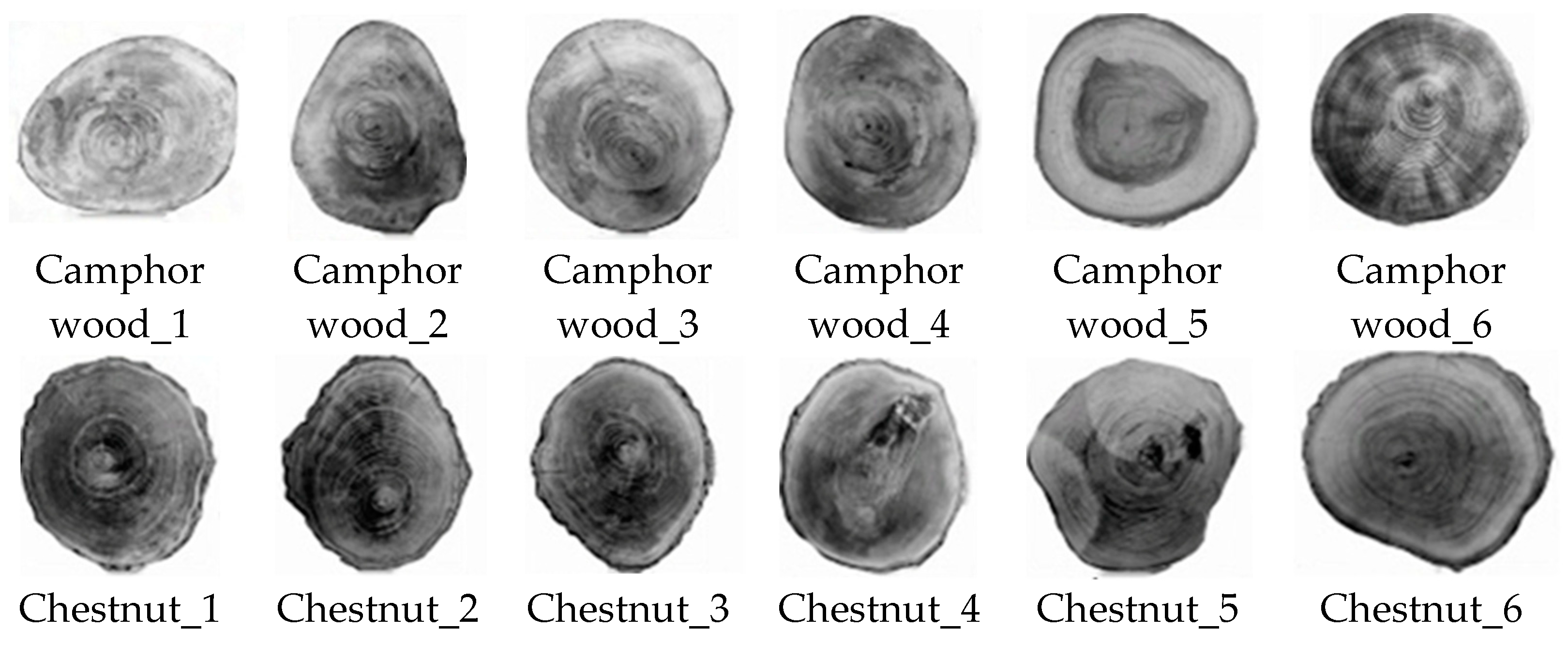
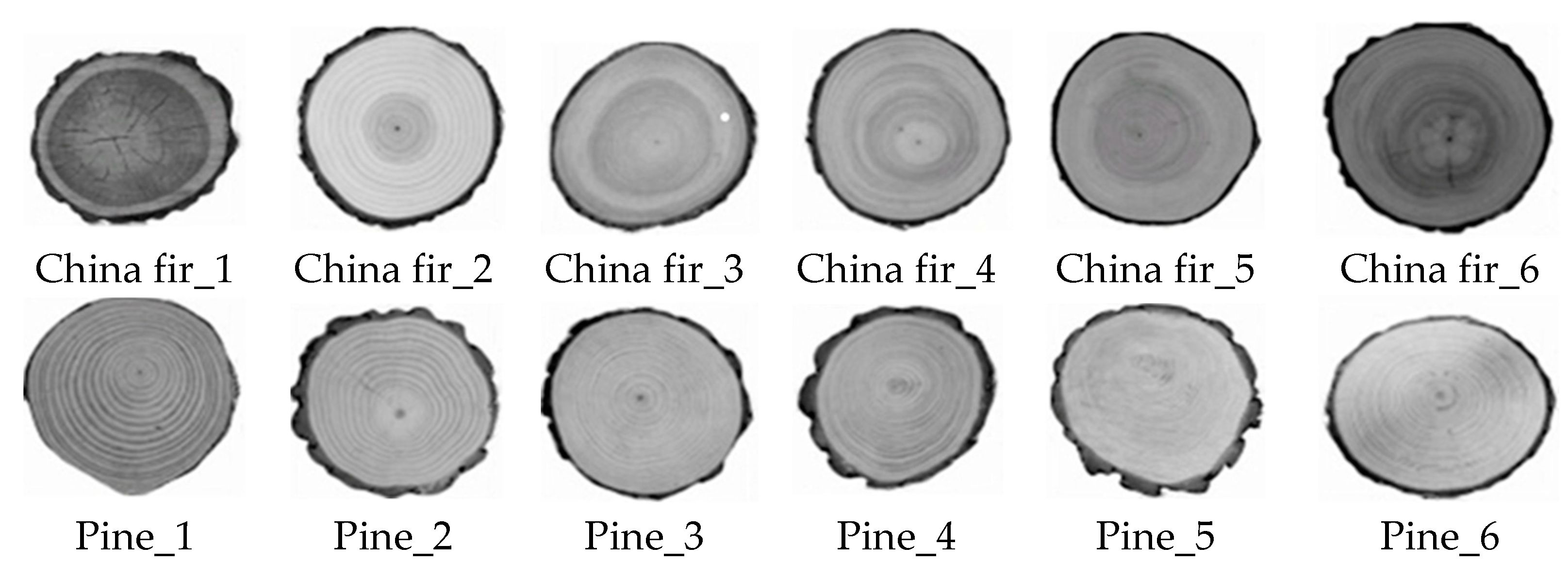
• Image acquisition of tree discs

The discs of four different species of trees were adopted as the research samples in this paper, including camphorwood, chestnut, China fir and pine. These tree species are widely distributed in China and are common wood raw material. Accordingly, a total of 12 transverse-cutting sample discs were employed for each species and the digital images were mostly obtained from the internet and a small part were obtained by the camera. Some samples are shown in Figure 1.

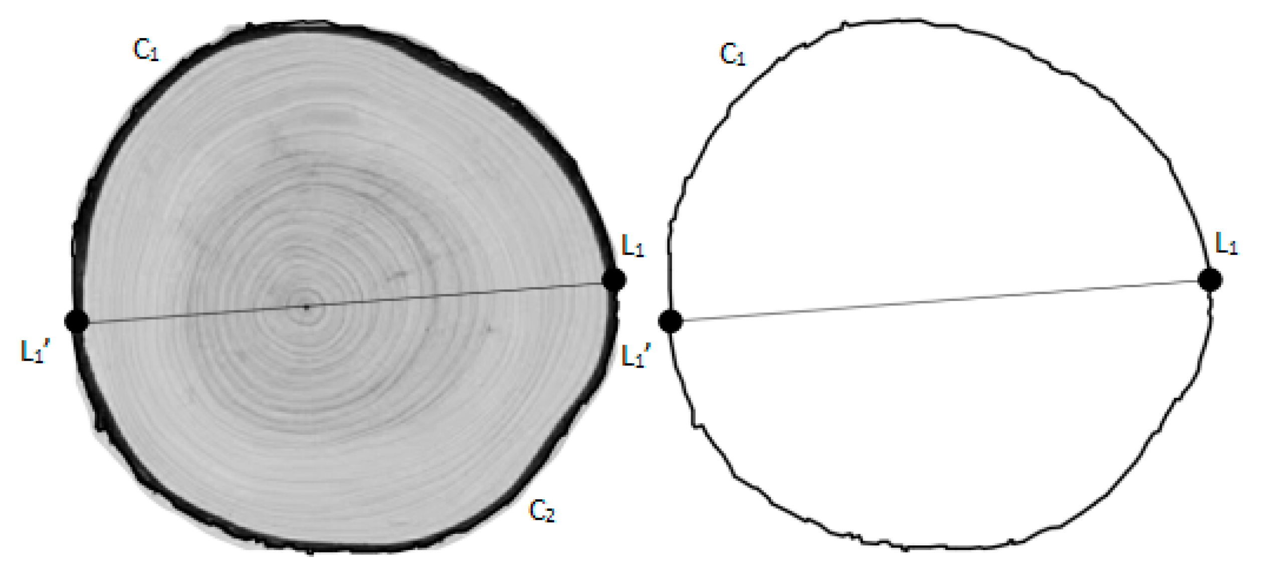
• Verification of geometric properties

1 Finding the longest chord through the pith

Sample images were shown in Figure 2. After sample images were imported into AutoCAD, the pith positions were marked manually. Then, as shown in Figure 3, many relatively long chords through the pith were assumed, measured and compared. Finally, the longest chord passing through the pith on the tree disc was obtained.

2 Perimeter measurement

In order to measure the length of every part of the outer contour of the tree disc, split by the longest chord through the pith, polylines were respectively made on the two parts, based on the principle of cyclotomy.

As shown in Figure 4, the outer-contour circumference, C was segmented into C₁ and C₂. ΔC is defined as the length difference between C₁ and C₂. ΔC of samples of different species are shown in

Table 1. Value ΔC ¹ of different species.

Species	1	2	3	4	5	6	7	8	9	10	11	12
camphorwood	3.91	4.66	0.56	6.07	3.63	0.88	3.71	0.99	4.43	6.18	2.52	7.58
chestnut	7.33	1.54	2.78	8.58	3.12	4.64	3.43	0.21	6.66	1.66	1.90	0.51
China fir	7.75	0.02	1.25	7.74	1.01	1.72	1.40	4.39	5.90	2.13	2.29	6.39
pine	2.60	2.82	2.56	3.94	0.97	6.75	6.28	2.40	8.15	0.94	2.45	3.64

¹ The units of measurement in this table are cm.

.

$$\begin{array}{c}C=C_1+C_2\\ \mathsf{\Delta }C=\left|C_1-C_2\right|\end{array}$$

(1)

3 t-test

Single sample t-test was used to analyze whether there was length difference between the two parts of the outer-contour circumference, split by the longest chord passing through the pith. The result of t-test shows that the significance of all species is less than 0.05, that is, the longest chord passing through the pith cannot bisect the outer-contour circumference without any error. In order to obtain the permissible error range, the range of ΔC and 95% confidence interval were analyzed, as shown in

Table 2. 95% confidence interval of value ΔC of different species.

Species	Mean Value (cm)	Lower Limit of 95% Confidence Interval (cm)	Upper Limit of 95% Confidence Interval (cm)
camphorwood	3.76	2.34	5.18
chestnut	3.53	1.80	5.26
China fir	3.86	1.77	5.94
pine	3.62	2.17	5.08

.

In order to make an overall estimate of the error range, the upper limit of 95% confidence interval was employed during the error analysis, and the error E is defined as the Formula (2). Error E of 12 samples in each species is shown in

Table 3. Error E of different species.

Species	1	2	3	4	5	6	7	8	9	10	11	12
camphor-wood	4.3%	3.8%	5.4%	4.7%	5.1%	4.9%	5.1%	4.4%	4.8%	5.9%	5.0%	4.2%
chestnut	5.3%	4.4%	5.0%	4.6%	5.7%	5.3%	5.2%	5.7%	5.2%	6.9%	4.3%	5.0%
China fir	4.1%	5.6%	4.0%	4.9%	4.7%	4.3%	6.6%	6.5%	4.0%	4.8%	4.7%	4.2%
pine	5.2%	6.3%	6.1%	5.9%	4.9%	4.2%	5.1%	4.2%	4.4%	6.8%	5.4%	4.9%

, and the 95% confidence interval of error E in each species is shown in

Table 4. 95% confidence interval of error E of different species.

Species	Mean Value	Lower Limit of 95% Confidence Interval	Upper Limit of 95% Confidence Interval
camphorwood	4.80%	4.44%	5.16%
chestnut	5.22%	4.78%	5.66%
China fir	5.47%	4.83%	6.10%
pine	5.28%	4.75%	5.82%

.

$$E=\frac{\mathsf{\Delta }{C}_{95\%\mathrm{upperlimit}} }{C}\times 100\%$$

(2)

From Table 3 and Table 4, it can be concluded that all the errors E of four different species are within 7%, lower than the permissible error range of 10% in this paper. Furthermore, single sample t-test with the test value of 5% was made to error E of each species samples. The result of t-test shows that the significance of all species is greater than 0.05, which means that there is no distinguished difference. Moreover, error E of samples of each species fluctuates around 5%, all of ΔC are within the permissible range of test error. Therefore, to an extent, the hypothesis about the geometric properties can be verified that the longest chord passing through the pith can bisect the outer-contour circumference of the tree disc within a permissible range of test error. In further research, more samples will be added to verify the geometric properties.

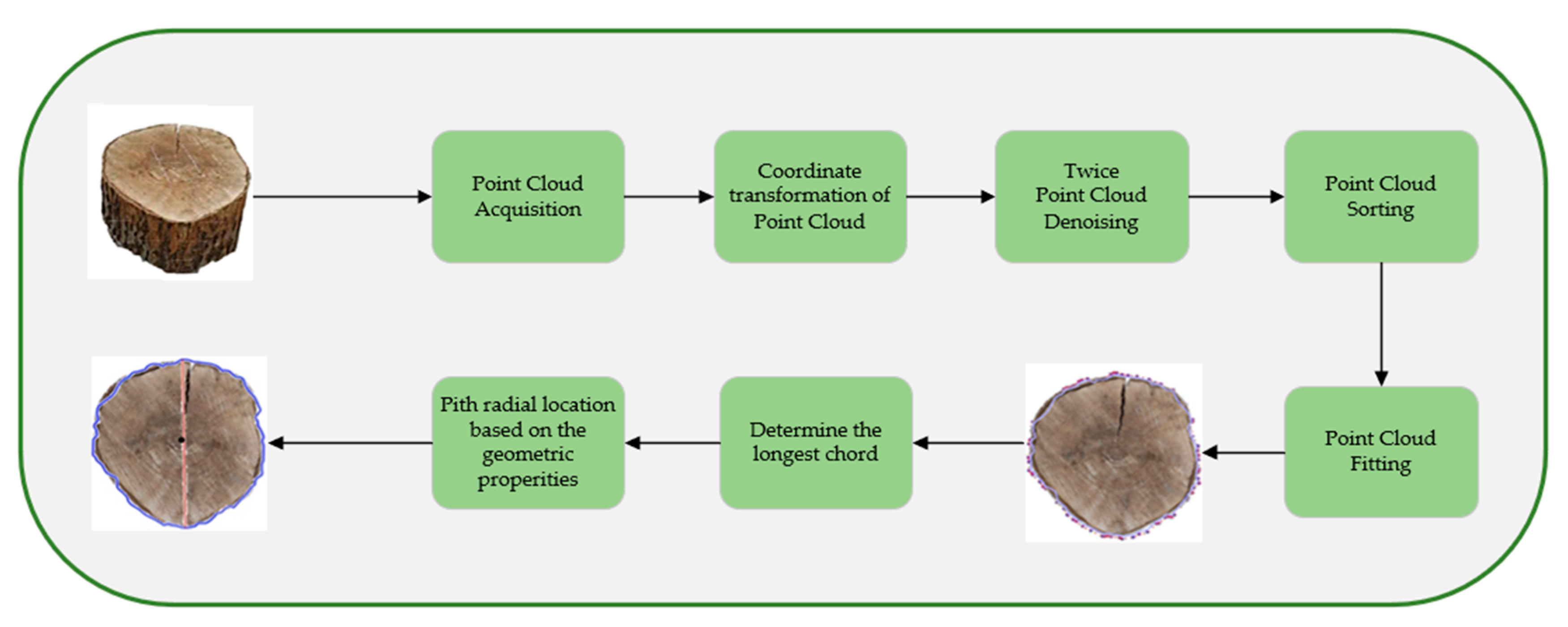
3. Materials and Methods

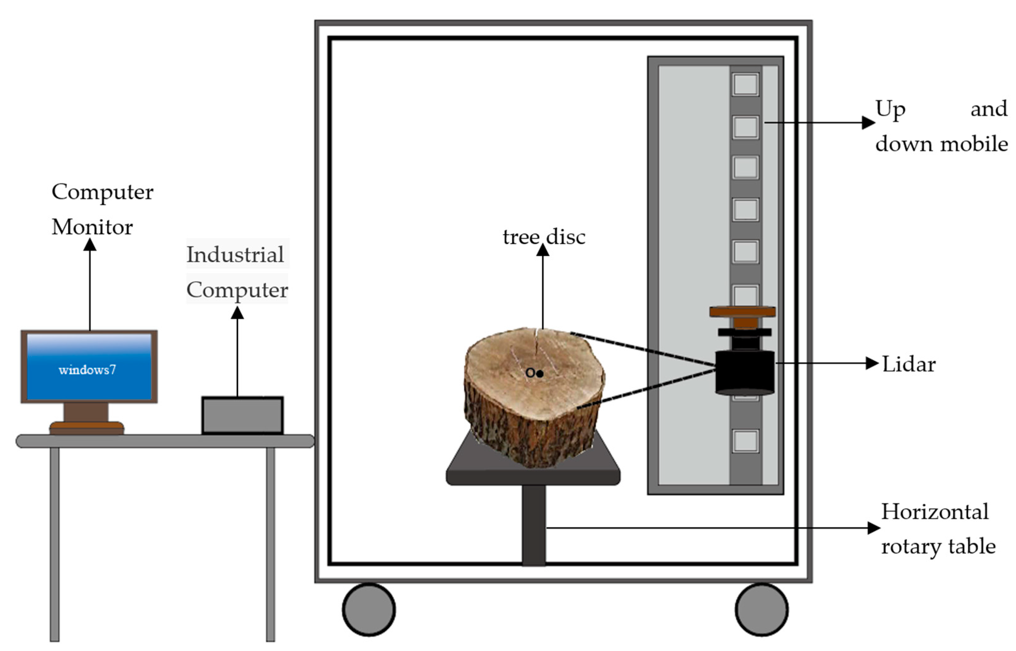
3.1. Data Acquisition

The data acquisition equipment is a 2D terrestrial laser scanner, SICK LMS141-15100 [28,29,30,31,32,33]. The laser lidar parameters are shown in

Table 5. The parameters of LMS 141-15100.

Parameters	Value
work area	0.5 m–40 m
operation temperature	−40 °C–+60 °C
working voltage	9 V DC–30 V DC
opening angle	270°
angular resolution	0.25°–0.5°
scanning frequency	25 Hz–50 Hz
response time	≥20 ms
measurement error	±12 mm (0.5 m–10 m) ±20 mm (10 m–20 m) ±35 mm (20 m–40 m)

. The experimental scene in the laboratory is shown in Figure 5. When using for standing trees in the field, the principle and the process are the same with that for tree discs. The tree disc was scanned at four points, including A, B, C, and D, with the same distance to O, the center of Square ABCD, as shown in Figure 6.

As seen in Figure 6, the position of the laser transmitter of LiDAR was regarded as the origin of the above-mentioned four coordinate systems, the direction orienting to the target disc as the direction of the positive axis X, and the direction of the positive axis Y was determined according to the right-hand rule. When the sample was scanned at points A, B, C, and D, $\left(x_{Ai},y_{Ai}\right)$,$\left(x_{Bi},y_{Bi}\right)$,$\left(x_{Ci},y_{Ci}\right)$ and $\left(x_{Di},y_{Di}\right)$ are defined as coordinates of the obtained data in the corresponding coordinate systems XAY, $X^{\prime }B{Y}^{\prime }$,$X^{″}C{Y}^{″}$ and $X^{‴}D{Y}^{‴}$.

After four-time scanning of the tree disc, the point cloud data obtained by the LiDAR are shown in Figure 7. The blue dots represent the scanning data of point A, the red dots represent the scanning data of point B, the green dots represent the scanning data of point C, and the yellow dots represent the scanning data of point D.

3.2. Data Processing

The flow chart of data processing is listed in Figure 8.

3.2.1. Point Cloud Coordinate Transformation

From the spatial position relationship among the four Cartesian coordinate systems, it can be inferred that the transformation relationship between the different coordinate systems [34]. As shown in Formulas (3)–(5), the transformation matrix, $T_B^A$, $T_C^A, T_D^A$respectively means the matrix to transform the point cloud in the coordinate system $X^{\prime }B{Y}^{\prime }$, $X^{″}C{Y}^{″}$,$X^{‴}D{Y}^{‴}$ to the coordinate system XAY.

$$T_B^A=\left|\begin{array}{ccc}{\mathit{cos}90}^{°}& {\mathit{sin}90}^{°}& \frac{\sqrt{2}}{2}L\\ {-\mathit{sin}90}^{°}& {\mathit{cos}90}^{°}& \frac{\sqrt{2}}{2}L\\ 0& 0& 1\end{array}\right|$$

(3)

$$T_C^A=\left|\begin{array}{ccc}{\mathit{cos}180}^{°}& {\mathit{sin}180}^{°}& L\\ {-\mathit{sin}180}^{°}& {\mathit{cos}180}^{°}& 0\\ 0& 0& 1\end{array}\right|$$

(4)

$$T_D^A=\left|\begin{array}{ccc}{\mathit{cos}(-90}^{°})& {\mathit{sin}(-90}^{°})& \frac{\sqrt{2}}{2}L\\ {-\mathit{sin}(-90}^{°})& {\mathit{cos}(-90}^{°})& -\frac{\sqrt{2}}{2}L\\ 0& 0& 1\end{array}\right|$$

(5)

After transforming all the scanning data to the coordinate system XAY, the visualization results of four-time scanning data are displayed in Figure 9.

3.2.2. Point Cloud Denoising

Because there are lots of noise data in the raw data, denoising of point cloud in this paper was divided into two steps. First, the gross error was removed. According to the scanning principle of LiDAR, the measuring angle of the marginal part of LiDAR is bigger than the central one, so that there was a relatively large error in the marginal data compared with the central data, which led to the distortion of the marginal data. This paper filtered out the most marginal point cloud, and the first-step denoising result is shown in Figure 10.

The second-step denoising made use of the distance threshold method [35,36,37]. That is to say, the data obtained from four-time scanning were grouped to denoise, according to the different scanning positions. Since the curve of each group of data is approximately arc-like, when the points on the arc satisfied Formula (6) were retained. Otherwise, they were filtered out, and the second-step denoising result is presented in Figure 11.

$$\{\begin{array}{c}0.95\overline{d}\le d_i\le 1.05\overline{d}\\ \frac{\overline{d}=\left({\sum }_{i=1}^n{d}_i\right)}{n}\end{array}$$

(6)

where d_i is defined as the distance between the data point and the center point O, $\overline{d}$ means the average distance of the group, and n is the number of collected point cloud.

3.2.3. Point Cloud Sorting

The order of point cloud plays an important role in curve reconstruction [38]. The ant colony algorithm was employed to sort the denoised data. As seen in Figure 12a, the connected polygon of the unsorted point cloud is relatively unsmooth, and the connected sequence of several data points is obviously wrong. After sorting by the ant colony algorithm [39,40,41], it can be seen that the connected order of the point cloud is significantly improved in Figure 12b.

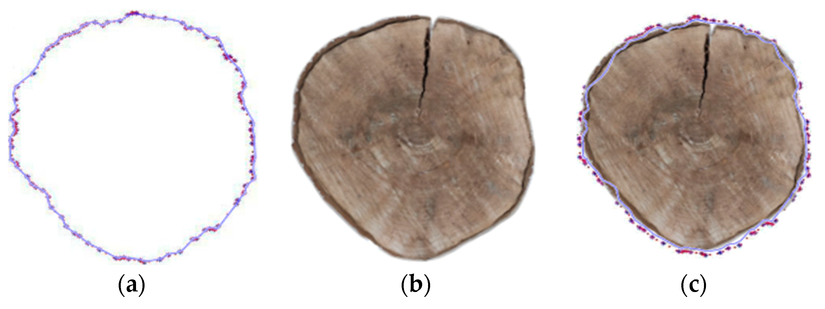
3.3. Point Cloud Fitting of Cross-Section Contour

In this paper, cubic spline curves were adopted to interpolate point cloud data of cross-section outline under the cyclic boundary condition [42,43,44]. The data visualization results after interpolation are shown in Figure 13. The blue-marked points are the original data, and the red-marked points are 200 interpolation points.

The point cloud data were connected to generate the outer-contour fitting curve of the cross-section, as shown in the blue line of Figure 13. Compared with the real contour of the disc, it can be found that both are basically coincident, indicating that the performance of interpolation and curve-fitting are good.

3.4. Pith Localization in Radial Direction

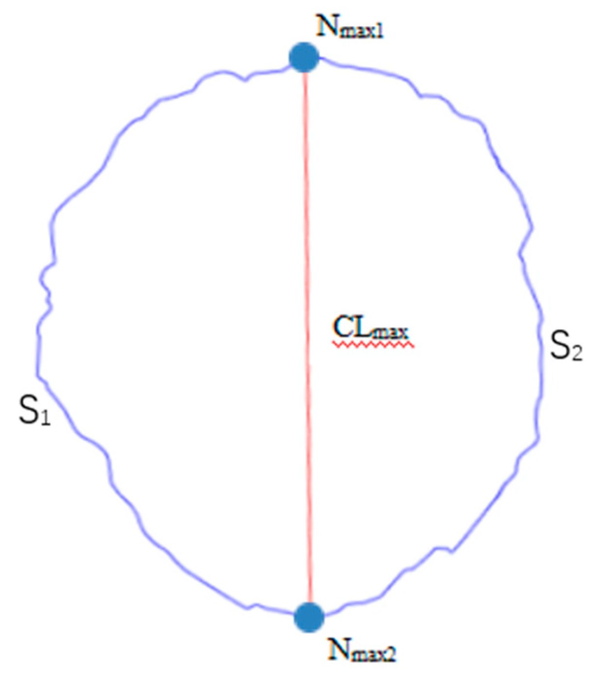
3.4.1. Finding the Longest Chord

As shown in Formula (7), the chord lengths between two points were calculated and then the longest chord on the cross-section was obtained.

$${\mathit{CL}}_i=\sqrt{{\left(x_{i+1}{-x}_i\right)}^2+{\left(y_{i+1}{-y}_i\right)}^2}$$

(7)

where $\left(x_i,y_i\right)$and $\left(x_j,y_j\right)$ are any two points, and CL_i is defined as the chord length between the corresponding two points. As seen in Figure 14, CL_max, with the two endpoints N_max1 and N_max2, is the longest chord, assumed to pass through the pith.

3.4.2. The Radial Location of the Pith

Supposed the fitting perimeter of the disc’s cross-section is S, the perimeter of the two parts, segmented by the assumed longest chord, is respectively S₁ and S₂. The fitting curve is divided into several sub-intervals, composed of two adjacent points on the curve. As seen in Figure 15, the length of the curve in each sub-interval is $\Delta S_i$ and the length of the straight line is $\Delta L_i$, and the differences of x-coordinate and y-coordinate at the endpoints are separately dx and dy. The length of the curve in each sub-interval is simplified as the length of the straight line between the two endpoints. It can be expressed as Formulas (8) and (9).

$$\Delta S_i\approx \Delta L_i=\sqrt{{\mathit{dx}}^2{+\mathit{dy}}^2}$$

(8)

$${S=S}_1{+S}_2={\displaystyle \sum }\Delta S_i\approx {\displaystyle \sum }\Delta L_i$$

(9)

Based on the calculation results of S₁ and S₂, if the longest chord could not bisect the circumference of the cross-section, it was concluded that this chord does not pass through the pith. The second longest chord on the cross-section need to be searched until a longer chord conforming to the geometric properties, that is, bisecting the circumference, was found. Consequently, the radial direction of the pith was located.

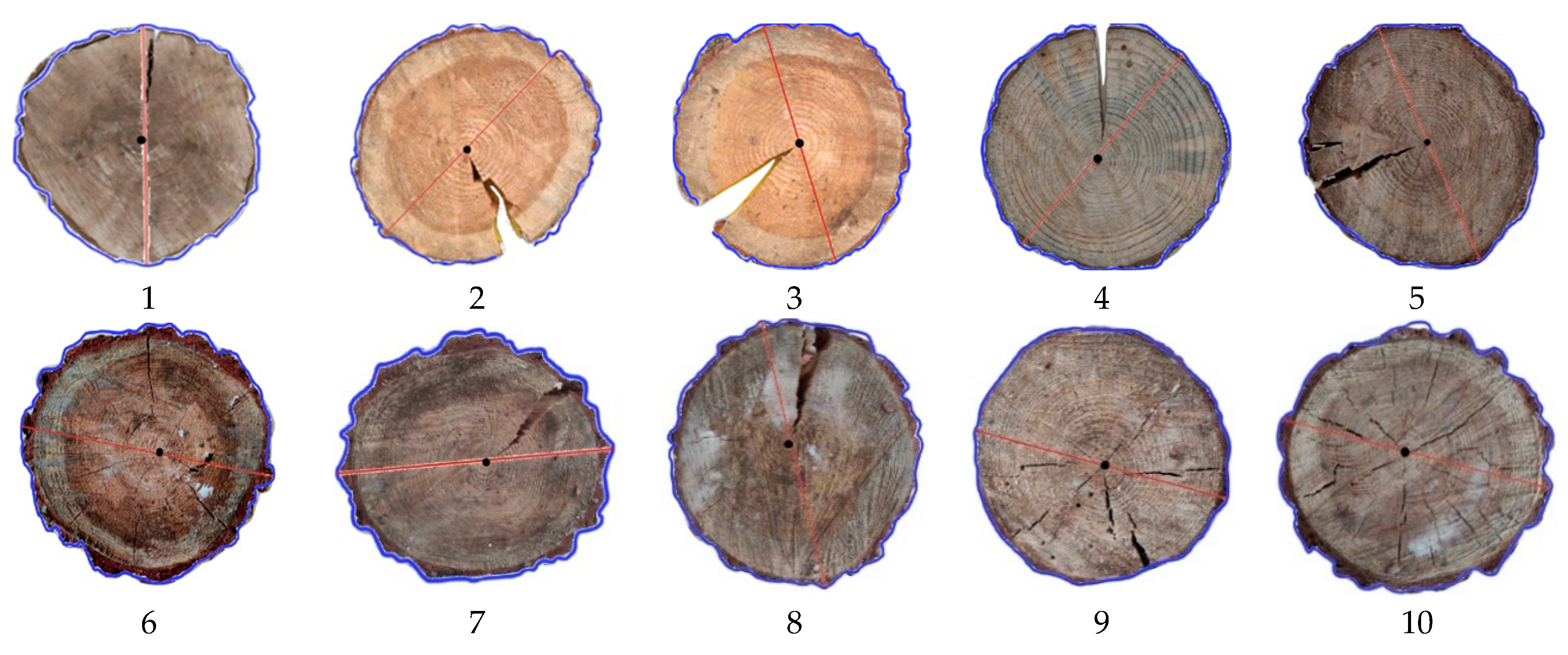
4. Experiment and Analysis

In this paper, discs were employed to make location experiments out of cross-section because the visible pith made it easier to evaluate the location performance. Due to water loss over time, half of 10 tree discs had cracks as shown in Figure 16. In order to make sure that the above-mentioned geometric properties of tree pith apply to the cracked tree discs, error E of ΔC, the length difference between the two outer-contour circumferences, split by the longest chord passing through the pith, was calculated for the digital images of 10 tree discs. The results are shown in

Table 6. Error E of the ten discs.

Samples.	1	2	3	4	5	6	7	8	9	10
ΔC (cm)	1.46	1.17	4.56	5.59	2.24	1.48	5.93	0.72	1.04	0.31
E	2.7%	2.4%	2.3%	4.6%	4.4%	3.7%	3.9%	4.7%	4.4%	3.8%

.

In Table 6, all the errors of ΔC of 10 tree discs are lower than 5%, that is, the geometric properties of tree pith work for 10 tree discs. Therefore, 10 tree disc samples were tested outside of the cross-section for radial pith location based on LiDAR. The results are shown in

Table 7. Experimental results of different samples.

Samples	1	2	3	4	5	6	7	8	9	10
ECL	0.17%	0.21%	1.27%	3.65%	1.29%	0.48%	1.45%	1.44%	3.00%	1.46%

. The error E_CL of the two-part outer contour circumference, S₁ and S₂, is defined as Formula (10).

$$E_{\mathit{CL}}=\frac{\left|S_1{-S}_2\right|}{S}\times 100\%$$

(10)

According to the regulation for trees with DBH (diameter at breast height) greater than 20 cm in ‘the Technical Regulations on Continuous Inventory of National Forest Resources’ (State Forestry Administration, 2014), the DBH measurement error is required to be less than 1.5%. Therefore, the permissible error range in this paper is defined to be 1.5%.

CL_max of Sample 8 and 10 through the pith is respectively the second and third longest one of all the chords on the cross-section, and CL_max of all the other samples through the pith are the longest chord. As shown in Table 7, except for Sample 4 and 9, E_CL errors of other samples are less than 1.5%, and the minimum error is only 0.17%. That is, for the other eight samples except Samples 4 and 9, the radial location of the pith can be achieved by finding the longest chord that bisects the circumference of the cross-section contour of the disc. On the cross-sections of Samples 4 and 9, the first five longest chords bisect the circumference of the cross-section outer contour of the disc with an error of more than 1.5%.

A comparison was made between the experimental result and the ground truth of the sample discs, as shown in Figure 16. The red line means the chord passing through the pith obtained by the experiment, and the black dot was marked manually, representing the real pith of the disc. In Figure 16, it was concluded that all the CL_max obtained by this method passed through the pith O on the cross-section of the sample discs. In Sample 4 and 9, CL_max also passed through the real pith, although the bisectional effect of the circumference of the cross-section outer contour was not ideal.

By comparing the cross-section shapes of all the sample discs, it was found that the cross-section shapes of Sample 4 and 9 are more similar to circles, while other samples are more similar to ellipses. For the disc with the oval cross-section, the method proposed in this paper can be used to locate the radial direction of the pith in trees discs. However, for the disc with the circle-like cross-section shape, the longest chord on the cross-section would pass through the pith to implement radial location, and it is not necessary to verify whether this chord has the geometric property of bisecting the cross-section perimeter.

5. Conclusions

In this paper, the geometric property of the pith was first proposed and verified, that is, the longest chord passing through the pith, can bisect the circumference of cross-section outline of the disc within a certain error range. On this basis, a radial location method of the pith based on terrestrial laser scanning was put forward. Two-dimensional LiDAR was used to scan tree discs to obtain data. Then, coordinate transformation, denoising, sorting, and interpolation of the point cloud were carried out, and the longest chords bisecting the cross-section perimeter were obtained to locate the radial direction of the pith. Through experimental verification and comparative analysis on tree discs, for the tree disc whose cross-section shape is close to ellipse, the error of the method proposed in this paper is less than 1.5%.

References

1. Youming, X. Wood Science; China Forestry Press: Beijing, China, 2006. [Google Scholar]
2. Jianju, L.; Jinyang, L.V. The structure of tree pith and its aesthetic application. J. South. Agric. 2012, 43, 1367–1372. [Google Scholar]
3. Cao, T.; Valsta, L.; Harkonen, S.; Saranpää, P.; Mäkelä, A. Effects of thinnin and fertilization on wood properties and economic return for Norway spruce. For. Ecol. Manag. 2008, 256, 1280–1289. [Google Scholar] [CrossRef]
4. Ikami, Y.; Murata, K.; Matsumura, Y.; Tsuchikawa, S. Influence of pith location on warp of lumber in sawing medium-quality sugi (Cryptomeria japonicaD. Don) logs. Eur. J. Wood Wood Prod. 2009, 67, 271–276. [Google Scholar] [CrossRef]
5. Jie, C. Application of Image Processing Technology and Statistical Method in Automatic Tree Ring Analysis System. Ph.D. Thesis, Xi′an University of Electronic Science and Technology, Xi′an, China, 2013. [Google Scholar]
6. Longuetaud, F.; Leban, J.-M.; Mothe, F.; Kerrien, E.; Berger, M.-O. Automatic detection of pith on ct images of spruce logs. Comput. Electron. Agric. 2004, 44, 107–119. [Google Scholar] [CrossRef]
7. Arx, G.V.; Dietz, H. Automated image analysis of annual rings in the roots of perennial forbs. Int. J. Plant. Sci. 2005, 166, 723–732. [Google Scholar] [CrossRef]
8. Bhandarkar, S.; Faust, T.D.; Tang, M. A system for detection of internal log defects by computer analysis of axial ct images. In Proceedings of the IEEE Workshop on Applications of Computer Vision, Sarasoto, FL, USA, 2–4 December 1996; pp. 258–263. [Google Scholar]
9. Boukadida, M.; Longuetaud, F.; Colin, F.; Freyburger, C.; Constant, T.; Leban, J.M.; Mothe, F. Pith Extract: A robust algorithm for pith detection in computer tomography images of wood Application to 125 logs from 17 tree species. Comput. Electron. Agric. 2012, 85, 90–98. [Google Scholar] [CrossRef]
10. Zhu, D.; Conners, R.W. A prototype vision system for analyzing ct imagery of hardwood logs. IEEE Trans. Syst. Man Cybern. Part B 1996, 26, 522–532. [Google Scholar] [CrossRef]
11. Longuetaud, F.; Saint-Andr, L.; Leban, J.M. Automatic detection of annual growth units on Picea abies Logs Using Optical and X-Ray Techniques. J. Nondestruct. Eval. 2005, 24, 29–43. [Google Scholar] [CrossRef]
12. Gazo, R.; Chang, J. Hardwood Log CT scanning—Proof of Concept. In Proceedings of the Joint UNECE Timber Committee Session and Society of Wood Science and Technology International Convention: Innovative Wood Products are the Future, United Nations, Geneva, Switzerland, 11–14 October 2010. [Google Scholar]
13. Gazo, R.; Vanek, J.; Abdul_Massih, M.; Benes, B. A fast pith detection for computed tomography scanned hardwood logs. Comput. Electron. Agric. 2020, 170, 105–107. [Google Scholar] [CrossRef]
14. Entacher, K.; Hegenbart, S.; Kerschbaumer, J.; Lenz, C.; Planitzer, D.; Seidel, M.; Uhl, A.; Weiglmaier, R. Pith Detection on CT-Cross-Section Images of Logs: An Experimental Comparison. In Proceedings of the International Symposium on Communications, Saint Julian’s, Malta, 12–14 March 2008; IEEE: Piscataway, NJ, USA, 2008. [Google Scholar]
15. Alkan, S. Industrial Computed Tomography (CT) Scanning of Subalpine Fir Logs: Proof of Concept; Forintek Canada Corp.: Vancouver, Canada, March 2003. [Google Scholar]
16. Perlin, L.P.; do Valle, Â.; Pinto, R.C.D.A. New method to locate the pith position in a wood cross-section based on ultrasonic measurements. Constr. Build. Mater. 2018, 169, 733–739. [Google Scholar] [CrossRef]
17. Altman, J.; Dolezal, J.; Čížek, L. Age estimation of large trees: New method based on partial increment core tested on an example of veteran oaks. For. Ecol. Manag. 2016, 380, 82–89. [Google Scholar] [CrossRef]
18. Kurdthongmee, W. A comparative study of the effectiveness of using popular dnn object detection algorithms for pith detection in cross-sectional images of parawood. Heliyon 2020, 6, e03480. [Google Scholar] [CrossRef] [PubMed] [Green Version]
19. Tongwen, Z.; Shulong, Y.; Yuting, F.; Heli, Z.; Ruibo, Z.; Huaming, S.; Li, Q.; Shengxia, J.; Feng, C. A Calibration Instrument for Measuring the Core Direction of the Growth Cone. CN208937368U, 4 June 2019. [Google Scholar]
20. Bucur, V. Nondestructive Characterization and Imaging of Wood; Springer: Berlin/Heidelberg, Germany, 2003. [Google Scholar]
21. Jianxun, L.; Dan, L.; Jinqiu, Q.; Xingyan, H.; Feng, L. Study on wood ring width and anatomical morphological characteristics of Toona sinensis. J. Southwest For. Univ. 2015, 35, 95–99. [Google Scholar]
22. Qijing, L. Application of digital photos in tree trunk analysis. J. Ecol. 2008, 3, 484–490. [Google Scholar]
23. Wu, M.; Xiangdon, L.; Guang, X.; Yingjun, Y.; Quanjun, W. Study on growth model of Quercus mongolica natural forest—IV. Growth model of entering boundary. J. Northwest Univ. Agric. For. Sci. Technol. (Nat. Sci. Ed.) 2015, 43, 58–64. [Google Scholar]
24. Jinqiu, Q.; Jianfeng, H.; Jiulong, X.; Bingling, W.; Hao, L. Study on radial variation of ring width and tracheid morphology of Metasequoia glyptostroboides. Guangxi Plants 2014, 34, 27–33. [Google Scholar]
25. Huning, W.; Tao, W. Discussion on the research progress of tree age determination method. Green Sci. Technol. 2013, 7, 152–155. [Google Scholar]
26. Juanjuan, Z.; Zhicheng, G.; Fang, S.; Yaming, Z. Research on tree ring width measurement based on digital image method. Ind. Instrum. Autom. 2017, 6, 75–77. [Google Scholar] [CrossRef]
27. Xingwen, B.; Luo, X.; Shubin, L. Application of AutoCAD in analyzing digital photos of wood disc. For. Resour. Manag. 2013, 2, 145–148. [Google Scholar] [CrossRef]
28. Leeuwen, M.V.; Nieuwenhuis, M. Retrieval of forest structural parameters using LiDAR remote sensing. Eur. J. For. Res. 2010, 129, 749–770. [Google Scholar] [CrossRef]
29. Liang, X.; Litkey, P.; Hyyppa, J.; Kaartinen, H.; Vastaranta, M.; Holopainen, M. Automatic Stem Mapping Using Single-Scan Terrestrial Laser Scanning. IEEE Trans. Geosci. Remote Sens. 2012, 50, 661–670. [Google Scholar] [CrossRef]
30. Lovell, J.; Jupp, D.; Newnham, G.; Culvenor, D. Measuring tree stem diameters using intensity profiles from ground-based scanning lidar from a fixed viewpoint. ISPRS J. Photogramm. Remote Sens. 2011, 66, 46–55. [Google Scholar] [CrossRef]
31. Ekevad, M. Method to compute fiber directions in wood from computed tomography images. J. Wood Sci. 2004, 50, 41–46. [Google Scholar] [CrossRef]
32. Raumonen, P.; Kaasalainen, M.; Åkerblom, M.; Kaasalainen, S.; Kaartinen, H.; Vastaranta, M.; Holopainen, M.; Disney, M.; Lewis, P. Fast automatic precision tree models from terrestrial laser scanner data. Remote Sens. 2013, 5, 491–520. [Google Scholar] [CrossRef] [Green Version]
33. Schraml, R.; Uhl, A. Pith estimation on rough log end images using local Fourier spectrum analysis. In Proceedings of the 14th Conference on Computer Graphics and Imaging (CGIM’13), Innsbruck, Austria, 12 February 2013. [Google Scholar]
34. Xiaoyue, W.; Shizhou, Y.; Changzhi, Z.; Guangtian, C. Research and application of data point sorting algorithm of section line. Mech. Manuf. Autom. 2009, 38, 58–59. [Google Scholar]
35. Yaohui, L. Implementation of three threshold calculation methods in Matlab 6.5. J. Xiangnan Univ. 2007, 5, 81–84. [Google Scholar] [CrossRef]
36. Ya, W.; Xinhua, L.; Haifeng, W. An improved wavelet threshold denoising method and its implementation in MATLAB. Microcomput. Inf. 2006, 6, 266–268. [Google Scholar]
37. Xinming, Z.; Lansun, S.; Bo, S. Thresholding method based on feature distance and its application in ophthalmic image segmentation. Chin. J. Image Graph. 2001, 6, 159–163. [Google Scholar] [CrossRef]
38. Tannert, T.; Anthony, R.W.; Kasal, B.; Kloiber, M.; Piazza, M.; Riggio, M.; Rinn, F.; Widmann, R.; Yamaguchi, N. In Situ assessment of structural timber using semi-destructive techniques. Mater. Struct. 2014, 47, 767–785. [Google Scholar] [CrossRef]
39. Kurdthongmee, W.; Suwannarat, K. Locating Wood Pith in a Wood Stem Cross Sectional Image Using YOLO Object Detection. In Proceedings of the 2019 International Conference on Technologies and Applications of Artificial Intelligence (TAAI), Kaohsiung, Taiwan, 1 November 2019. [Google Scholar]
40. Feng, S.; Zhou, H.; Dong, H. Using deep neural network with small dataset to predict material defects. Mater. Des. 2019, 162, 300–310. [Google Scholar] [CrossRef]
41. Matlab Chinese Forum. Analysis of 30 Cases of MATLAB Neural Network; Beijing University of Aeronautics and Astronautics Press: Beijing China, 2010. [Google Scholar]
42. Du, X.; Li, S.; Li, G.; Feng, H.; Chen, S. Stress Wave Tomography of Wood Internal Defects using Ellipse-Based Spatial Interpolation and Velocity Compensation. Bioresources 2015, 10. [Google Scholar] [CrossRef]
43. Feng, H.; Li, G.; Fu, S.; Wang, X. Tomographic Image Reconstruction Using an Interpolation Method for Tree Decay Detection. Bioresources 2014, 9, 3248–3263. [Google Scholar] [CrossRef]
44. Xiaoyong, X.; Taiyong, Z. Construction of cubic spline interpolation function and its implementation in MATLAB. Ordnance Autom. 2006, 25, 76–78. [Google Scholar] [CrossRef]
Figure 1. Digital images of some samples.
Forests 12 00671 g001aForests 12 00671 g001b
Figure 2. Sample images of cross-section of lumber.
Forests 12 00671 g002
Figure 3. Drawing the longest chord passing through the pith.
Forests 12 00671 g003
Figure 4. Measuring the perimeter of tree disk.
Forests 12 00671 g004
Figure 5. Experimental scene diagram.
Forests 12 00671 g005
Figure 6. Diagrammatic sketch of data collection.
Forests 12 00671 g006
Figure 7. Point cloud data obtained from four-time scanning.
Forests 12 00671 g007
Figure 8. Data processing flow chart.
Forests 12 00671 g008
Figure 9. Data visualization after coordinate transformation.
Forests 12 00671 g009
Figure 10. The first-step denoising.
Forests 12 00671 g010
Figure 11. The result of the second-step denoising.
Forests 12 00671 g011
Figure 12. Comparison of point cloud connections before and after sorting. (a) Point cloud connection before sorting; (b) Point cloud connection after sorting.
Forests 12 00671 g012
Figure 13. Comparison of point cloud fitting contour and cubic spline interpolation contour. (a) Interpolation results and fitting contour; (b) True disc contour; (c) Comparison chart.
Forests 12 00671 g013
Figure 14. The longest chord CLmax on the cross-section.
Forests 12 00671 g014
Figure 15. Parameters of the sub-interval segment.
Forests 12 00671 g015
Figure 16. The radial location experimental results of the pith.
Forests 12 00671 g016