The Effect of Post-Fire Disturbances on a Seasonally Thawed Layer in the Permafrost Larch Forests of Central Siberia

 ,
,  ,
,  ,
,
Abstract
1. Introduction
2. Materials and Methods
2.1. Study Area
2.2. Remote Sensing Data on Wildfires and Post-Fire Plots
2.3. Data on Soils and STL Influenced by Natural Conditions
2.4. Numerical Simulation of The STL’s Thickness under the Conditions of the Post-Fire Plots
3. Results
3.1. Characteristics of Fire-Disturbed Areas from Remote Sensing Data
3.2. Regression Model of STL
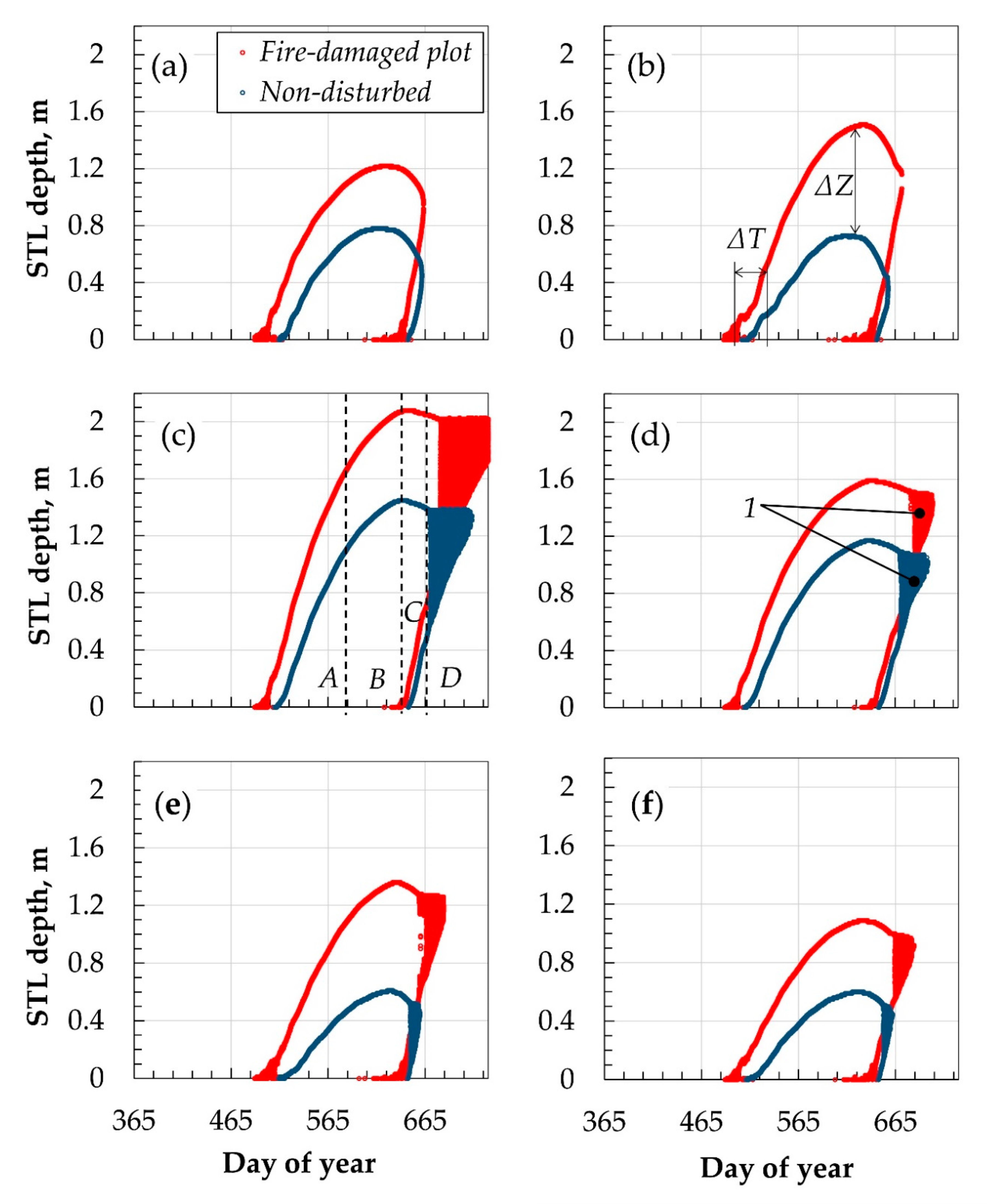
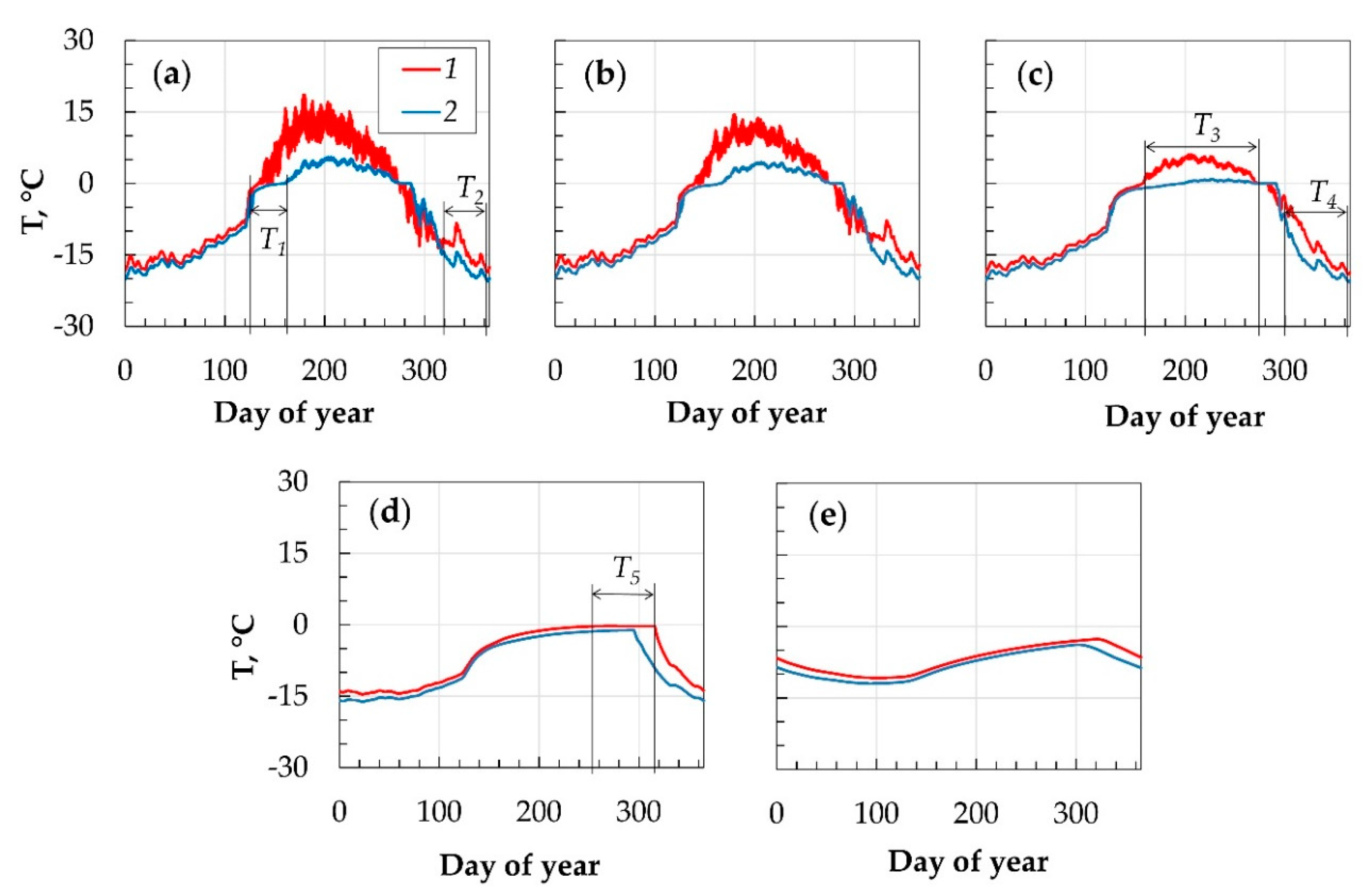
3.3. Simulated Annual Dynamics of Soil Temperature and STL Depth
4. Discussion
4.1. Fire Disturbances and Post-Fire Effects
4.2. Statistical Data on STL and Regression Model
4.3. Numeric Simulation of Soil Temperature and STL Depth
4.4. Limitations
- (1)
- The speed of loss of NDVI deviation, as well as the temperature deviation, should be mediated by fire severity, drainage, stand density, etc. However, in the current study, we did not attempt to quantify such relations.
- (2)
- Accounting for the movement of water in the soil is the primary purpose of further developments of the mathematical model. The vertical movement of moisture associated with precipitation, snow melting and the evaporation of moisture from the surface can make a significant contribution to the heat transfer in the soil. Moisture transfer can be significantly different depending on the presence of fire damage, since the damaged and intact organic layer differs in its ability to accumulate moisture.
- (3)
- The simulation was carried out under the assumption that plots were damaged by fire recently, in cases of the complete degradation of the moss–lichen cover and disturbance of the forest stand. The complete absence of the upper organic layer (Opir) was assumed in the model for fire-damaged soils. All these remain a topic for future research, and further validations of simulation results are also required.
5. Conclusions
Supplementary Materials
Author Contributions
Funding
Conflicts of Interest
References
- Ponomarev, E.I.; Ponomareva, T.V. The Effect of Postfire Temperature Anomalies on Seasonal Soil Thawing in the Permafrost Zone of Central Siberia Evaluated Using Remote Data. Contemp. Probl. Ecol. 2018, 11, 420–427. [Google Scholar] [CrossRef]
- Kharuk, V.I.; Ponomarev, E.I. Spatiotemporal Characteristics of Wildfire Frequency and Relative Area Burned in Larch-dominated Forests of Central Siberia. Rus. J. Ecol. 2017, 48, 507–512. [Google Scholar] [CrossRef]
- Abaimov, A.P.; Sofronov, M.A. The main trends of post-fire succession in near-tundra forests of central Siberia. In Fire in Ecosystems of Boreal Eurasia; Goldammer, J.G., Furyaev, V.V., Eds.; Kluwer Academic Publishers: Dordrecht, The Netherlands, 1996; pp. 372–386. [Google Scholar]
- Gorbachev, V.N.; Popova, E.P. Fires and soil formation. In Fire in Ecosystems of Boreal Eurasia; Goldammer, J.G., Furyaev, V.V., Eds.; Kluwer Academic Publishers: Dordrecht, The Netherlands, 1996; pp. 331–336. [Google Scholar]
- Sofronov, M.A.; Volokitina, A.V.; Kajimoto, T.; Matsuura, Y.; Uemura, S. Zonal peculiarities of forest vegetation controlled by fires in northern Siberia. Eurasian J. For. Res. 2000, 1, 51–59. [Google Scholar]
- Anisimov, O.A. Potential feedback of thawing permafrost to the global climate system through methane emission. Environ. Res. Lett. 2007, 2, 045016. [Google Scholar] [CrossRef]
- Desyatkin, R.V.; Desyatkin, A.R. Temperature Regime of Solonetzic Meadow-Chernozemic Permafrost-Affected Soil in a Long-Term Cycle. Eurasian Soil Sci. 2017, 50, 1301–1310. [Google Scholar] [CrossRef]
- Park, H.; Launiainen, S.; Konstantinov, P.Y.; Iijima, Y.; Fedorov, A.N. Modeling the effect of moss cover on soil temperature and carbon fluxes at a tundra site in northeastern Siberia. J. Geophys. Res. Biogeosci. 2018, 123, 3028–3044. [Google Scholar] [CrossRef]
- Sofronov, M.A.; Volokitina, A.V.; Kajimoto, T. Ecology of wildland fires and permafrost: Their interdependence in the northern part of Siberia. In Proceedings of the Eighth Symposium on the Joint Siberian Permafrost Studies between Japan and Russia in 1999, Tsukuba, Japan, 19–20 January 2000; pp. 211–218. [Google Scholar]
- Anisimov, O.A.; Sherstiukov, A.B. Evaluating the effect of environmental factors on permafrost in Russia. Kriosf. Zemli (Earth’s Cryosphere) 2016, 2, 78–86. (In Russian) [Google Scholar]
- Masyagina, O.V.; Menyailo, O.V. The impact of permafrost on carbon dioxide and methane fluxes in Siberia: A meta-analysis. Environ. Res. 2020, 182, 109096. [Google Scholar] [CrossRef]
- Knorre, A.A.; Kirdyanov, A.V.; Prokushkin, A.S.; Krusic, P.J.; Büntgen, U. Tree ring-based reconstruction of the long-term influence of wildfires on permafrost active layer dynamics in Central Siberia. Sci. Total Environ. 2019, 652, 314–319. [Google Scholar] [CrossRef]
- Orgogozo, L.; Prokushkin, A.S.; Pokrovsky, O.S.; Grenier, C.; Quintard, M.; Viers, J.; Audry, S. Water and energy transfer modeling in a permafrost dominated, forested catchment of Central Siberia: The key role of rooting depth. Permafr. Periglac. Process. 2019, 30, 75–89. [Google Scholar] [CrossRef]
- Kirdyanov, A.V.; Prokushkin, A.S.; Tabakova, M.A. Tree-ring growth of Gmelin larch in the north of Central Siberia under contrasting soil conditions in the north of Central Siberia. Dendrochronologia 2013, 31, 114–119. [Google Scholar] [CrossRef]
- Desyatkin, R.V.; Desyatkin, A.R.; Fedorov, P.P. Temperature regime of taiga cryosoils of Central Yakutia. Kriosf. Zemli (Earth Cryosphere) 2012, 16, 70–78. (In Russian) [Google Scholar]
- Lebedeva, L.S.; Semenova, O.M.; Vinogradova, T.A. Calculation of the depth of seasonally melted layer in various landscapes of Kolyma water-balance station based on Gidrograf hydrological model. Kriosf. Zemli (Earth Cryosphere) 2015, 19, 35–44. [Google Scholar]
- Viereck, L.A. Effects of fire and firelines on active layer thickness and soil temperature in interior Alaska. In Proceedings of the Fourth Canadian Permafrost Conference, Calgary, Alberta, 2–6 March 1981; Frech, H.M., Ed.; National Research Council Canada: Ottawa, ON, Canada, 1982; pp. 123–135. [Google Scholar]
- Dyrness, C.T.; Viereck, L.A.; van Cleve, K. Fire in taiga communities of Interior Alaska. In Forest Ecosystems in the Alaskan Taiga; Van Cleve, K., Chapin, F.S., III, Flanagan, P.W., Viereck, L.A., Dyrness, C.T., Eds.; Ecological Studies; Springer: Berlin, Germany, 1986; Volume 57, pp. 74–86. [Google Scholar]
- Wein, R.W.; Bliss, L.C. Changes in arctic Eriophorum Tussock communities following fire. Ecology 1973, 54, 845–852. [Google Scholar] [CrossRef]
- Rouse, W.R. Microclimatic changes accompanying burning in subarctic lichen woodland. Arct. Alp. Res. 1976, 4, 357–376. [Google Scholar] [CrossRef]
- Landhäusser, S.M.; Wein, R.W. Postfire vegetation recovery and tree establishment at the arctic treeline: Climate-change-vegetation-response hypotheses. J. Ecol. 1993, 81, 665–672. [Google Scholar] [CrossRef]
- Brown, J.; Ferrians, O.J.; Heginbottom, J.A.; Melnikov, E.S. Circum-Arctic Map of Permafrost and Ground Ice Conditions, Ver. 2; National Snow and Ice Data Center. Digital Media: Boulder, CO, USA, 2002. Available online: https://nsidc.org/data/ggd318 (accessed on 22 June 2020).
- Masyagina, O.; Prokushkin, A.; Kirdyanov, A.; Artyukhov, A.; Udalova, T.; Senchenkov, S.; Rublev, A. Intraseasonal carbon sequestration and allocation in larch trees growing on permafrost in Siberia after 13C labeling (two seasons of 2013–2014 observation). Photosynth. Res. 2016, 130, 267–274. [Google Scholar] [CrossRef]
- Masyagina, O.V.; Evgrafova, S.Y.; Titov, S.V.; Prokushkin, A.S. Dynamics of soil respiration at different stages of pyrogenic restoration succession with different-aged burns in Evenkia as an example. Russ. J. Ecol. 2015, 46, 27–35. [Google Scholar] [CrossRef]
- World Reference Base for Soil Resources. 2014. Available online: https://www.isric.org/explore/wrb (accessed on 19 March 2020).
- Wild, B.; Schnecker, J.; Bárt, J.; Čapek, P.; Guggenberger, G.; Hofhansl, F.; Kaiser, C.; Lashchinsky, N.; Mikutta, R.; Mooshammer, M.; et al. Nitrogen dynamics in Turbic Cryosols from Siberia and Greenland. Soil Biol. Biochem. 2013, 67, 85–93. [Google Scholar] [CrossRef]
- Shishov, L.L.; Tonkonogov, V.D.; Lebedeva, I.I.; Gerasimova, I.I. Classification Diagnosis of Russian Soils; Oikumena: Smolensk, Russia, 2004; 341p. (In Russian) [Google Scholar]
- Startsev, V.V.; Dymov, A.A.; Prokushkin, A.S. Soils of Postpyrogenic Larch Stands in Central Siberia: Morphology, Physicochemical Properties, and Specificity of Soil Organic Matter. Eurasian Soil Sci. 2017, 50, 885–897. [Google Scholar] [CrossRef]
- Bezkorovaynaya, I.N.; Borisova, I.V.; Klimchenko, A.V.; Shabalina, O.M.; Zakharchenko, L.P.; Il’in, A.A.; Beskrovny, A.K. Influence of the pyrogenic factor on the biological activity of the soil under permafrost conditions (Central Evenkia). Vestnik KrasGAU 2017, 9, 181–189. (In Russian) [Google Scholar]
- Babichev, A.P.; Babushkina, N.A.; Bratkovskiy, A.M. Physical Quantities: Reference; Grigoryev, I.S., Meilikhova, Z.E., Eds.; Energoatomizdat: Moscow, Russia, 1991; 1232p. (In Russian) [Google Scholar]
- Sobol, V.R.; Goman, P.N.; Dedyulya, I.V.; Brovka, A.G.; Mazurenko, O.N. Thermal properties of the ground forest material with a characteristic moisture content. J. Eng. Phys. Thermophys. 2011, 84, 1079–1087. (In Russian) [Google Scholar]
- Gavrilyev, R.I.; Zheleznyak, M.N.; Zhilin, V.I.; Kirillin, A.R.; Zhirkov, A.F.; Pazynych, A.V. Thermophysical properties of the main types of rocks of the Elkonsky massif. Kriosfera Zemli (Earth’s Cryosphere) 2013, 17, 76–82. (In Russian) [Google Scholar]
- Gubin, S.V.; Lupachev, A.V. Suprapermafrost Horizons of the Accumulation of Raw Organic Matter in Tundra Cryozems of Northern Yakutia. Eurasian Soil Sci. 2018, 51, 772–781. [Google Scholar] [CrossRef]
- Ponomarev, E.I.; Shvetsov, E.G. Satellite detection of forest fires and geoinformation methods of calibration of the results. Issled Zemli Kosmosa (Rem. Sens.) 2015, 1, 84–91. (In Russian) [Google Scholar] [CrossRef]
- Giglio, L.; Descloitres, J.; Justice, C.; Kaufman, Y. An enhanced contextual fire detection algorithm for MODIS. Remote Sens. Environ. 2003, 87, 273–282. [Google Scholar] [CrossRef]
- Shvetsov, E.G. Probabilistic Approach of Satellite Detection and Assessment of Fire Energy Characteristics in Forests of East Siberia. Ph.D. Thesis, V.N. Sukachev Institute of Forest, Krasnoyarsk, Russia, 2012. (In Russian). [Google Scholar]
- Vermote, E.; Wolfe, R. MOD09GQ MODIS/Terra Surface Reflectance Daily L2G Global 250 m SIN Grid V006; NASA EOSDIS LP DAAC: Washington, DC, USA, 2015. [CrossRef]
- Wan, Z.; Hook, S.; Hulley, G. MOD11A1 MODIS/Terra Land Surface Temperature/Emissivity Daily L3 Global 1km SIN Grid V006; NASA EOSDIS LP DAAC: Washington, DC, USA, 2015. [CrossRef]
- Kornienko, S.G. Transformation of tundra land cover at the sites of pyrogenic disturbance: Studies based on LANDSAT satellite data. Kriosfera Zemli (Earth’s Cryosphere) 2017, 21, 93–104. [Google Scholar]
- Lunardini, V.J. Heat Transfer with Freezing and Thawing; Elsevier: Radarweg, The Netherlands, 1991; 65p. [Google Scholar]
- Nourgaliev, R.R.; Dinh, T.N.; Haraldsson, H.O.; Sehgal, B.R. The multiphase Eulerian-Lagrangian transport (MELT-3D) approach for modeling of multiphase mixing in fragmentation processes. Prog. Nucl. Energy 2003, 42, 123–157. [Google Scholar] [CrossRef]
- Oke, T.R. Boundary Layer Climates, 2d ed.; Routledge: London, UK, 1987; 435p. [Google Scholar]
- Psiloglou, B.E.; Santamouris, M.; Asimakopoulos, D.N. Atmospheric Broadband Model for Computation of Solar Radiation at the Earth’s Surface. Application to Mediterranean Climate. Pure Appl. Geophys 2000, 157, 829–860. [Google Scholar] [CrossRef]
- Pavlov, A.V. Thermal Physics of Landscapes; Nauka: Novosibirsk, Russia, 1979; 285p. (In Russian) [Google Scholar]
- Pavlov, A.V. Cryolithozone Monitoring; Geo: Novosibirsk, Russia, 2008; 229p. (In Russian) [Google Scholar]
- Climatic Research Unit. Available online: http://www.cru.uea.ac.uk/ (accessed on 19 March 2020).
- Weather Archive. Available online: http://rp5.ru (accessed on 19 March 2020).
- NNDC Climate Data. Available online: http://www7.ncdc.noaa.gov/CDO/cdo (accessed on 19 March 2020).
- Tarnawski, V.R.; Leong, W.H.; Bristow, K.L. Developing a temperature-dependent Kersten function for soil thermal conductivity. Int. J. Energy Res. 2000, 24, 1335–1350. [Google Scholar] [CrossRef]
- Semenov, S.M. Methods of Assessment of Climate Change Consequences for Physical and Biological Systems; Gidrometeoizdat: Moscow, Russia, 2012; 509p. (In Russian) [Google Scholar]
- Ekici, A.; Beer, C.; Hagemann, S.; Boike, J.; Langer, M. Simulating high-latitude permafrost regions by the JSBACH terrestrial ecosystem model. Geosci. Model. Dev. 2014, 7, 631–647. [Google Scholar] [CrossRef]
- Porada, P.; Ekici, A.; Beer, C. Effects of bryophyte and lichen cover on permafrost soil temperature at large scale. Cryosphere 2016, 10, 2291–2315. [Google Scholar] [CrossRef]
- Johansen, O. Thermal Conductivity of Soils. Ph.D. Thesis, University of Trondheim, Trondheim, Norway, 1975; 236p. [Google Scholar]
- Anisimov, O.A.; Anokhin, Y.A.; Lavrov, S.A.; Malkova, G.V.; Myach, L.T.; Pavlov, A.V.; Romanovskii, V.A.; Streletskii, D.A.; Kholodov, A.L.; Shiklomanov, N.I. Continental permafrost. In Methods of Assessment of Climate Change Consequences for Physical and Biological Systems; Semenov, S.M., Ed.; Gidrometeoizdat: Moscow, Russia, 2012; pp. 301–359. [Google Scholar]
- Kharuk, V.I.; Dvinskaya, M.L.; Ranson, K.J. Spatio-temporal dynamics of fires in the larch forests of the northern taiga of Central Siberia. Russ. J. Ecol. 2005, 5, 1–10. (In Russian) [Google Scholar]
- Ponomarev, E.I.; Kharuk, V.I.; Ranson, J.K. Wildfires Dynamics in Siberian Larch Forests. Forests 2016, 7, 125. [Google Scholar] [CrossRef]
- de Groot, W.J.; Cantin, A.S.; Flannigan, M.D.; Soja, A.J.; Gowman, L.M.; Newbery, A. A comparison of Canadian and Russian boreal forest fire regimes. For. Ecol. Manag. 2013, 294, 23–34. [Google Scholar] [CrossRef]
- Ponomarev, E.I.; Ponomareva, T.V.; Masyagina, O.V.; Shvetsov, E.G.; Ponomarev, O.I.; Krasnoshchekov, K.V.; Dergunov, A.V. Post-fire effect modeling for the permafrost zone in Central Siberia on the basis of remote sensing data. Proceedings 2019, 18, 2. [Google Scholar] [CrossRef]
- Shvetsov, E.G.; Ponomarev, E.I. Postfire Effects in Siberian Larch Stands on Multispectral Satellite Data. Contemp. Probl. Ecol. 2020, 13, 104–112. [Google Scholar] [CrossRef]
- Brown, D.R.N.; Jorgenson, M.T.; Kielland, K.; Verbyla, D.L.; Prakash, A.; Koch, J.C. Landscape Effects of Wildfire on Permafrost Distribution in Interior Alaska Derived from Remote Sensing. Remote Sens 2016, 8, 654. [Google Scholar] [CrossRef]
- Flannigan, M.; Stocks, B.; Turetsky, M.; Wotton, M. Impacts of climate change on fire activity and fire management in the circumboreal forest. Glob. Chang. Biol. 2009, 15, 549–560. [Google Scholar] [CrossRef]
- Valendik, E.N.; Kisilyakhov, E.K.; Ryzhkova, V.A.; Ponomarev, E.I.; Danilova, I.V. Conflagration fires in taiga landscapes of Central Siberia. Geogr. Nat. Resour. 2014, 35, 41–47. [Google Scholar] [CrossRef]


| Horizon | Depth, cm | Texture | Bulk Density, kg/m3 | Porosity | Specific Heat, J/(kg·K) |
|---|---|---|---|---|---|
| Control plots (non-disturbed soil) | |||||
| Oao | 0–12 | 60 | 0.91 | 1500 | |
| O(F+H) | 12–17 | 170 | 0.81 | 1880 | |
| CR | 17–35 | loamy | 1100 | 0.48 | 750 |
| C | 35–50 | loamy | 1600 | 0.36 | 920 |
| Postpyrogenic plots (fire-damaged soil) | |||||
| Opir | 0–2 | 180 | 0.74 | 1880 | |
| O(F+H)pir | 2–7 | 400 | 0.67 | 1000 | |
| CR | 7–25 | loamy | 1100 | 0.48 | 750 |
| C | 25–40 | loamy | 1600 | 0.36 | 920 |
| Soil Horizon | Qw | Qi | ||
|---|---|---|---|---|
| Non-Disturbed Plot | Fire-Damaged Plot | Non-Disturbed Plot | Fire-Damaged Plot | |
| Oao | 0.3 | NA * | 0.8 | NA * |
| O(F+H) | 0.35 | 0.14 | 0.79 | 0.55 |
| CR | 0.275 | 0.21 | 0.3 | 0.225 |
| C | 0.3 | 0.3 | 0.33 | 0.33 |
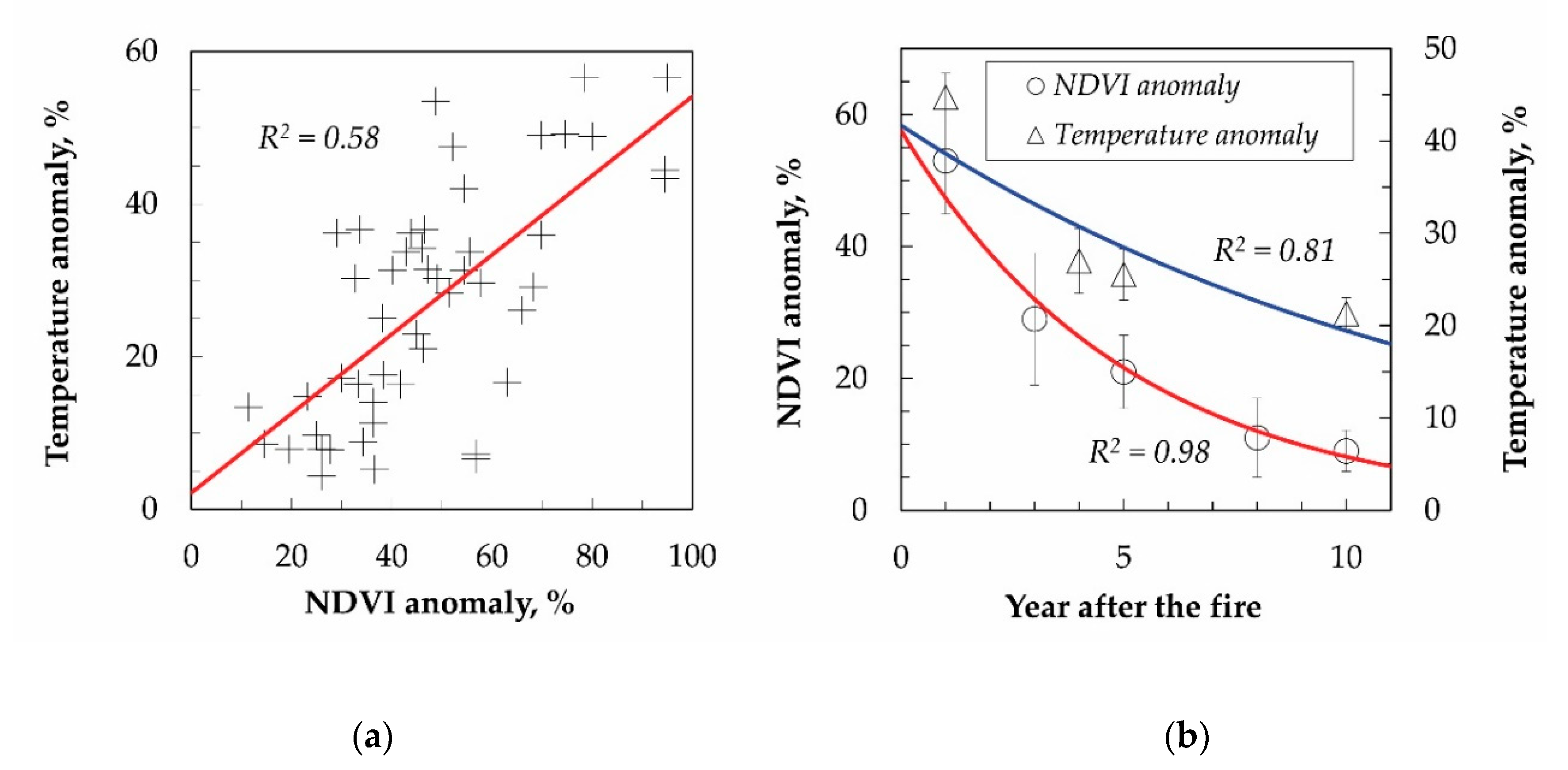
| Years after Fire | NDVI Anomaly, % | Range of Temperature Maximum, °C | Range of Temperature Anomaly, % |
|---|---|---|---|
| 1 | 53.5 ± 10.7 | 6.5−7.2 | 40–50 |
| 5 | 21.0 ± 7.8 | 3.8−4.9 | 27–32 |
| 10 | 9.0 ± 5.0 | 3.4−4.6 | 15–20 |
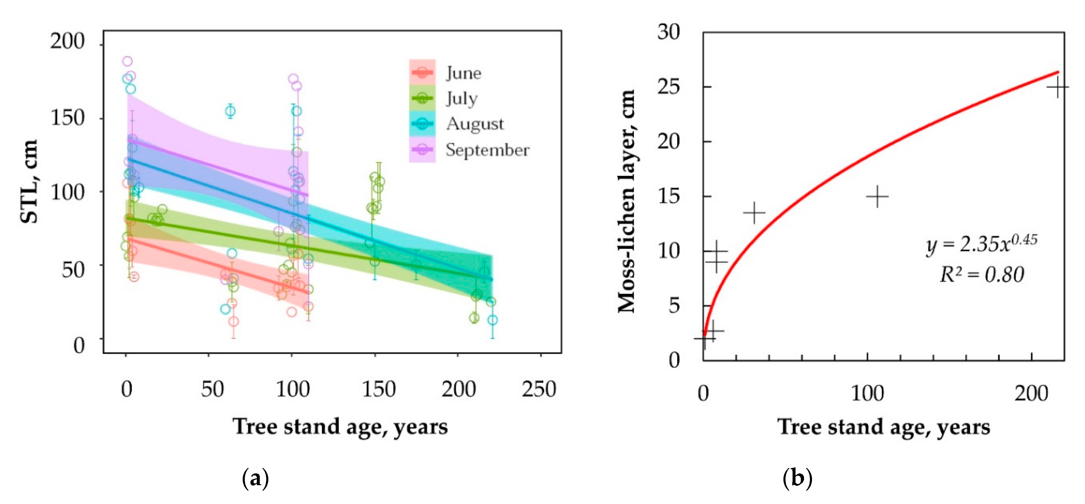
| Description | Coefficient | R2 Adjusted | p | df | |
|---|---|---|---|---|---|
| a | Intercept | 103.93 | 0.46 | <0.0001 | 70 |
| b | −0.18 | ||||
| c | −16.71 | ||||
| d | Coefficient for July | 22.88 | |||
| d | Coefficient for August | 41.13 | |||
| d | Coefficient for September | 40.42 | |||
| A | Data on tree stand age | ||||
| L | Data on soil organic layer (litter) | ||||
| t | Time step |
© 2020 by the authors. Licensee MDPI, Basel, Switzerland. This article is an open access article distributed under the terms and conditions of the Creative Commons Attribution (CC BY) license (http://creativecommons.org/licenses/by/4.0/).
Share and Cite
Ponomarev, E.; Masyagina, O.; Litvintsev, K.; Ponomareva, T.; Shvetsov, E.; Finnikov, K. The Effect of Post-Fire Disturbances on a Seasonally Thawed Layer in the Permafrost Larch Forests of Central Siberia. Forests 2020, 11, 790. https://doi.org/10.3390/f11080790
Ponomarev E, Masyagina O, Litvintsev K, Ponomareva T, Shvetsov E, Finnikov K. The Effect of Post-Fire Disturbances on a Seasonally Thawed Layer in the Permafrost Larch Forests of Central Siberia. Forests. 2020; 11(8):790. https://doi.org/10.3390/f11080790
Chicago/Turabian StylePonomarev, Evgenii, Oxana Masyagina, Kirill Litvintsev, Tatiana Ponomareva, Evgeny Shvetsov, and Konstantin Finnikov. 2020. "The Effect of Post-Fire Disturbances on a Seasonally Thawed Layer in the Permafrost Larch Forests of Central Siberia" Forests 11, no. 8: 790. https://doi.org/10.3390/f11080790
APA StylePonomarev, E., Masyagina, O., Litvintsev, K., Ponomareva, T., Shvetsov, E., & Finnikov, K. (2020). The Effect of Post-Fire Disturbances on a Seasonally Thawed Layer in the Permafrost Larch Forests of Central Siberia. Forests, 11(8), 790. https://doi.org/10.3390/f11080790