Article

Forest Phenology Shifts in Response to Climate Change over China–Mongolia–Russia International Economic Corridor

1
Northeast Institute of Geography and Agroecology, Chinese Academy of Sciences, Changchun 130012, China
2
College of Earth Science, Jilin University, Changchun 130102, China
*
Author to whom correspondence should be addressed.
Forests 2020, 11(7), 757; https://doi.org/10.3390/f11070757
Submission received: 21 May 2020 / Revised: 4 July 2020 / Accepted: 13 July 2020 / Published: 14 July 2020
(This article belongs to the Special Issue Effect of Climate Change on Forest Growth and Phenology)

Abstract

:
Vegetation phenology is a sensitive indicator of climate change. With the intensification of global warming, the changes in growing seasons of various vegetation types have been widely documented across the world. However, as one of the most vulnerable regions in response to the global climate change, the phenological responses and associated mechanisms in mid–high latitude forests are still not fully understood. In this study, long-term changes in forest phenology and the associated relationship with the temperature and snow water equivalent in the China–Mongolia–Russia International Economic Corridor were examined by analyzing the satellite-measured normalized difference vegetation index and the meteorological observation data during 1982 to 2015. The average start date of the growing season (SOS) of the forest ecosystem in our study area advanced at a rate of 2.5 days/decade, while the end date of the growing season (EOS) was delayed at a rate of 2.3 days/decade, contributing to a growing season that was approximately 15 days longer in the 2010s compared to that in 1980s. A higher April temperature is beneficial to the advance in the SOS, and a higher summer temperature has the potential to extend the EOS in the forest ecosystem. However, our results also suggest that a single temperature cannot fully explain the advance of the SOS, as well as the delay in the EOS. The preseason Snow Water Equivalent (SWE) is also an essential factor in influencing the growing season. A higher SWE in February and March and lower SWE in April tend to advance the SOS, while higher SWE in pre-year December and lower SWE in current year October are beneficial to the extension of the EOS.

1. Introduction

Vegetation phenology is a sensitive indicator of climate change [1,2,3,4,5]. The advance or delay of the growing season reflects the long-term biological impacts of climate on the terrestrial ecosystem and, as a result, influences the productivity of the ecosystem [6]. Temperature records, as well as model simulations, show that global temperatures have increased obviously and significantly, especially in mid and high latitudes since the beginning of the 20th century [7,8,9]. Over the past several decades, both field observations and satellite records showed an extension of the growing season at regional and global scales [10,11,12].
Remote sensing measurements are capable of providing continuous spatiotemporal information and have become the most commonly used tool to monitor the phenology variations at large scales in recent decades [13]. Previous studies have investigated phenology variations in the Northern Hemisphere based on a series of remote sensing datasets [11,14,15,16,17]. Among the datasets, the long-term Advanced Very High-Resolution Radiometer (AVHRR) Normalized difference vegetation index (NDVI) dataset since 1981 provides the most commonly used data to detect phenology events on both continental and global scales. Based on this long-term NDVI series, Stockli and Vidale found that the start date of the growing season (SOS) advanced by about 0.56 days per decade, while the end date of the growing season (EOS) was delayed by about 9.6 days per decade during 1982 to 2001 in Europe [2]. Jeong’s (2011) study found that the SOS advanced by 5.4 days and the EOS was delayed by 6.6 days in the temperate vegetation over the Northern Hemisphere from 1982 to 2008 [14]. The advance in the SOS, combined with the delayed EOS, contribute to the extension of the growing season.
The relationship between vegetation phenology and climate change has been widely documented on different temporal and spatial scales. Most studies have provided evidence that the warmer temperature unequivocally contributed to the progressive advance of the start date of the growing season (SOS) for various vegetation types over both temporal and boreal regions [13,14,15,18]. However, the magnitude of this consistent SOS advance varied across vegetation types, geographical locations, as well as investigation periods [13]. With respect to temperatures, other factors, such as soil moisture and precipitation, may help explain the vegetation’s phenological changes, particularly in arid regions [19,20]. Several studies also indicated the importance of snowmelt and snow depth in determining vegetation growth as the snow changes can directly influence the global energy and moisture balance, which have the potential to affect the vegetation phenology [21,22].
In the forest ecosystem, the relationship between phenological variations and temperature has been well studied. Forests tend to grow in relative moisture conditions and there is little evidence that precipitation has a significant influence on temperate or boreal forest phenology [23]. Snow is different from rainfall as, in the high-latitude environments, thicker snowpack can insulate the soil from extremely cold temperatures and can help hold the soil nutrients, which is beneficial for forest growth [22]. Grippa et al. (2005) found a significant positive correlation between snow depth and growing season NDVI over central Siberia [24]. However, little is known about the relative role of winter and spring snowpack and the possible lagged effects on the beginning or the end of the growing season in mid- and high-latitude forests. Though the changes in the end date of the growing season (EOS) also play a vital role in determining the length of the growing season, the variations in the EOS and its associated climatic driving mechanisms are still not fully identified in the forest ecosystem [14,23].
The China–Mongolia–Russia International Economic Corridor is one of the most crucial regions for the application of the Belt and Road Initiative, a global development strategy adopted by the Chinese government in 2013 involving infrastructure development and investments in nearly 70 countries and international organizations [25]. With seasonally varied snow covers, the ecological environment of the area is extremely sensitive to global climate change [9,26], which should be fully evaluated to achieve a win–win between ecology and economy. The forest phenology shifts are proven to be sensitive indictors reflecting climate change. Monitoring forest phenology changes and unveiling their corresponding relationships with climatic factors can provide an important reference for the evaluation of the investment environment in the China–Mongolia–Russia International Economic Corridor, which can help avoid ecological issues or risks and achieve sustainable development for the whole region. Therefore, the primary objective of this study was to evaluate the spatial distribution pattern, as well as the long-term variations in the SOS and EOS of the forest ecosystem over the China–Mongolia–Russia International Economic Corridor from 1982 to 2015, based on the Global Inventory Modeling and Mapping Studies (GIMMS) NDVI dataset. Combined with the climate observation data, the relationship between phenological variations and temperature was examined. Snow water equivalent (SWE) was selected as a critical latent factor in influencing forest phenology variation and further identifying the response mechanisms of forest phenology to climate change. This study can help us to understand the vegetation’s phenological variation and its associated climatic driving factors in mid–high latitude forests, which is helpful for predicting vegetation response to future climate change and improving the estimation of the ecosystem process and function.

2. Materials and Methods

2.1. Study Area

The China–Mongolia–Russia International Economic Corridor is located in North and Northeast Asia and ranges from 56° E to 141.5° E in longitude and from 37.3° N to 62° N in latitude, as shown in Figure 1. The China–Mongolia–Russia International Economic Corridor mainly covers three countries, namely Northeast and Inner Mongolia of China, Mongolia and the southern part of Siberia in Russia. The elevation of this study area ranges from −272 m to 4390 m. The climate of this region was characterized by a long period of snow-covered winter and a relatively short, mild summer. The climate records show that the annual average temperature ranges from −11 °C to 13 °C, and the yearly total precipitation ranges from 35 mm to 990 mm in this region. Forests are the dominant land cover types in the area. Forests in this region include four different vegetation types, specifically broadleaved deciduous, needleleaved evergreen, needleleaved deciduous and mixed forest, which are classified as European Space Agency (ESA) Climate Change Initiative (CCI) land cover products used in this study [27].
However, the mid- and high-latitude regions of the Northern Hemisphere have experienced extraordinary warming since the beginning of the 20th century—far higher than the global average level [9]. The warming here directly influences the snow cover, as well as the phenology stages, including the start or the end date of the growing season. Understanding the forest phenology changes, as well as the contributors in this area, is helpful in tracking the natural climate change and forecasting future forest shifts in the northern hemisphere.

2.2. Data

Global Inventory Modeling and Mapping Studies (GIMMS) normalized difference vegetation index (NDVI) time-series data, derived from the advanced very high-resolution radiometer (AVHRR) from 1982 to 2015, were used to detect the phenology changes in our study area [28]. Previous studies have reported that a 6–16 day temporal resolution of the satellite data can generate the optimal estimate of the phenological stages [29]. The temporal resolution of the GIMMS NDVI3g data is 15 days, and spatial resolution is 8 km, which is suitable for large-scale ground phenological monitoring. The dataset ranges from July 1981 to December 2015. To eliminate the uncertainty caused by the data quality, we used quality flags equal to 0 (best quality) and 1 (good quality) to select the good values for the phenology model. The fitting weight for best qualities was set to 1, and for the good quality pixels it was set to 0.5.
The 300 m resolution global land cover data series from 1992 to 2015 produced by the European Space Agency (ESA) Climate Change Initiative (CCI) were used to extract the forest distribution in our study area [27]. The CCI land cover data created for climate studies have been widely used to describe the vegetation patterns in previous studies [30,31,32]. To avoid the impact of land cover changes on the phenology variation, only the unchanged forest during 1992 to 2015 was analyzed in this paper. Due to fewer human activities, the land use and land cover changes were not significant from 1975 to 2010 in Siberia [33]. Although the land use changes were significant in Northeast China from the 1980s to 2000, the forests changes mainly concentrated on deforestation [34]. Based on the previous studies and the data availability, forest increase or conversion between different forest types from 1982 to 1991 were not taken into consideration in this study. To make sure the CCI land cover data could capture the spatial distribution for different forest types, we used the 1:4,000,000 vegetation map in Russia and the 1:1,000,000 vegetation map in China to qualitatively evaluate the CCI’s accuracy. The two datasets showed good consistency in the forest and open woodlands, especially for dark and light coniferous forests and broad-leaved forests. It should be noted that the CCI data described the spatial distribution of different forest types with a higher resolution.
Mean air temperature, maximum air temperature, minimum air temperature and precipitation from the year 1982 to the year 2015 were obtained from Climate Research Unit (CRU) TS4.3 monthly data with a spatial resolution of 0.5° [35]. The monthly SWE data in the same time period were obtained from GlobSnow SWE v2.0 data [36], which combine ground-based weather station data with satellite-based passive microwave measurements. We rescaled both the climate data and land cover data to 8 km using the bilinear spatial interpolation method to match the spatial resolution of the NDVI products.

2.3. Methods and Analyses

Logistic models have been commonly used to detect phenological events [15,37]. Logistic models have good conceptual coherency with biophysical inference in terms of being a “growth curve” and are the primary technique used to extract phenological information from satellite observation data [38]. The double logistic functions have proved to be an effective way to accurately monitor the ground phenological transition dates by optimally removing outliers and reducing noise in remote sensing time series data [39,40]. In this study, we used a double logistic function to fit the time series NDVI data for each year:
g ( t ; x 1 , x 2 , x 3 , x 4 ) = 1 1 + exp ( x 1 t x 2 ) 1 1 + exp ( x 3 t x 4 )
where x 1 and x 3 determine the position of the left and right inflection point, respectively, while x 2 and x 4 represent the rate of change at the corresponding inflection points. Based on our previous studies [41], we selected the dynamic thresholds of 0.2 and 0.3 to extract the start of the season (SOS) and the end of the season (EOS), respectively. Then, the length of the season can be obtained by subtracting the SOS from the EOS. As the SOS and EOS extraction from the first (1982) and the last (2015) year was not robust, the results between 1983 and 2014 were analyzed.
We used least square regression to detect the changing trend for the SOS and EOS from 1982 to 2015 at the pixel scale. Our previous study used this method to identify the change slope for the growing season in Northeast China, and detailed information about this method can be found in Yu et al. (2017) [41]. We evaluated the response of spring and autumn phenology to monthly temperatures and SWE based on the partial least-squares (PLS) regression (implemented in JMP 13, SAS Institute). PLS regression is demonstrated to be suitable for highly autocorrelated variables [18,20,42], such as monthly temperature or SWE, as used here. This analysis can provide both influence direction (model coefficients, MCs) and the importance of the independent variables (variable importance plot, VIP) in explaining the variation in the response variable [18,20,42]. We spatially averaged data for all forest pixels of the temperature and SWE, as well as phenology grids for this analysis. In this study, the MC and VIP values can reflect the direction and importance of monthly temperature and SWE in influencing the SOS and EOS.

3. Results

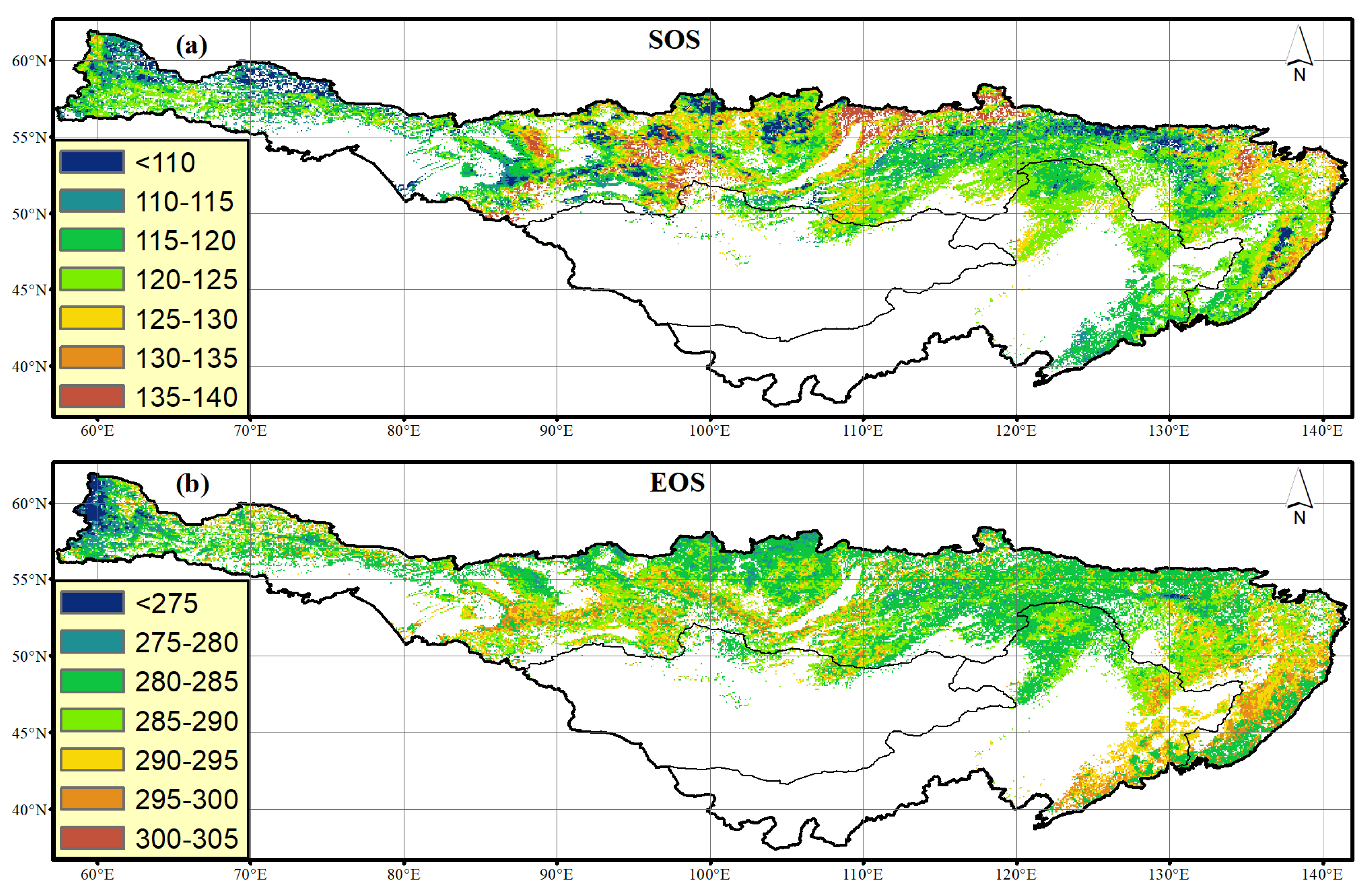
3.1. Characterization of Forest Phenology

The start date (SOS) and the end date (EOS)of the growing season across the forest in the China–Mongolia–Russia International Economic Corridor was detected by remote sensing during our studying period, as shown in Figure 2. On average, the SOS and EOS occurred on 120.8 ± 7.8 and 290.9 ± 9.5 Julian days across the forest landscape in the study area. The start and the end date of the growing season varied significantly across our study area, with some areas in the northwest beginning to green up before the 110th Julian day (20 April), while some areas north of Baikal and the mountain areas started to green up after the 135th Julian day (15 May). The end date of the growing season also showed remarkable spatial heterogeneity. The EOS of the west part of the economic corridor occurred before the 275th Julian day (5 October), while the EOS in the southernmost of the study area was close to late October. It should be noted that the SOS and EOS varied across different forests. The detailed SOS and EOS days are shown in Table 1.

3.2. Trends in Growing Season of Forest Phenology

To investigate the variations in forest phenology stages, we calculated the trend of the SOS and EOS from 1983 to 2014 at the pixel scale in our study area, as shown in Figure 3. The trend of the SOS, determined by the linear regression, was negative in approximately 95.7% of the forest, especially in the broadleaved deciduous forests and evergreen forests. The SOS trend was significantly negative (p < 0.05, t-test) in about 40.2% of the pixels, indicating significant advances in the SOS. The SOS advance exceeds 0.2 days/year, which is 6.4 days from 1983 to 2014, in nearly 41.7% of the area. Though the majority of pixels exhibited SOS advance, positive trends were also observed, and only 4.3% of the pixels showed an SOS delay during our study period. Significant spatial heterogeneity was also detected. Among the four forest types, the SOS advance in the broadleaved deciduous forest was the slowest, with 0.14 days/year, while the mixed forest showed the fastest SOS advances, which were 0.30 days/year on average.
In contrast to the SOS, the trend for the EOS was positive in 64.9% of the forests, indicating a delayed end of growing season, and 75.6% of which was significantly positive (p < 0.05, t-test). The EOS delay exceeded 0.2 days/year in nearly 55.8% of the forest area. Similar to the SOS, the changing trend in the EOS showed significant spatial distribution differences. Areas, such as the Greater Khingan Mountains and central Siberia, showed a delayed trend higher than 0.6, indicating that the end of the growing season was extended by more than 19 days. A negative EOS trend was mainly found in the north part of our study area, and the pixels with an advance in EOS account for 4.8% of the forest area.
To analyze the temporal trends in the SOS and EOS, we averaged the change slope over all pixels covered by forest, as shown in Figure 4c,d. The regional mean SOS over the forest in the China–Mongolia–Russia International Economic Corridor advanced over the past 32 years (R2 = 0.264, p = 0.0026), with an annual advance of 0.25 days per year, as shown in Figure 4c. The regional mean of the EOS was delayed by 7.3 days during our study period (R2 = 0.356, p = 0.0003), with a delay rate of 0.23 days per year, as shown in Figure 4d. To analyze the climate background change trend in this area, we calculated the annual average temperature and SWE for the forest grids. The regional mean temperature in this area increased at a rate of 0.019 °C/year from 1983 to 2014 (R2 = 0.071, p = 0.1407). The mean SWE increased 2.74 mm (R2 = 0.129, p = 0.0437), with an increased rate of 0.086 mm/year.
The regression analysis between the SOS and the climatic factors, including the annual average temperature and SWE, indicated negative sensitivity of SOS to temperature (R2 = 0.18, p = 0.0165). An increase in annual average temperature would advance the SOS by 2.81 days across the forest in our study area, indicating that the temperature plays an essential role in regulating the SOS. The observed EOS changes are not linear responses to temperature, meaning that the changes in EOS do not result from a monotonic vegetation response to temperature. To further investigate the climatic driving factors for the phenology changes, we used PLS regression to analyze the dominant variables in determining the SOS and EOS.

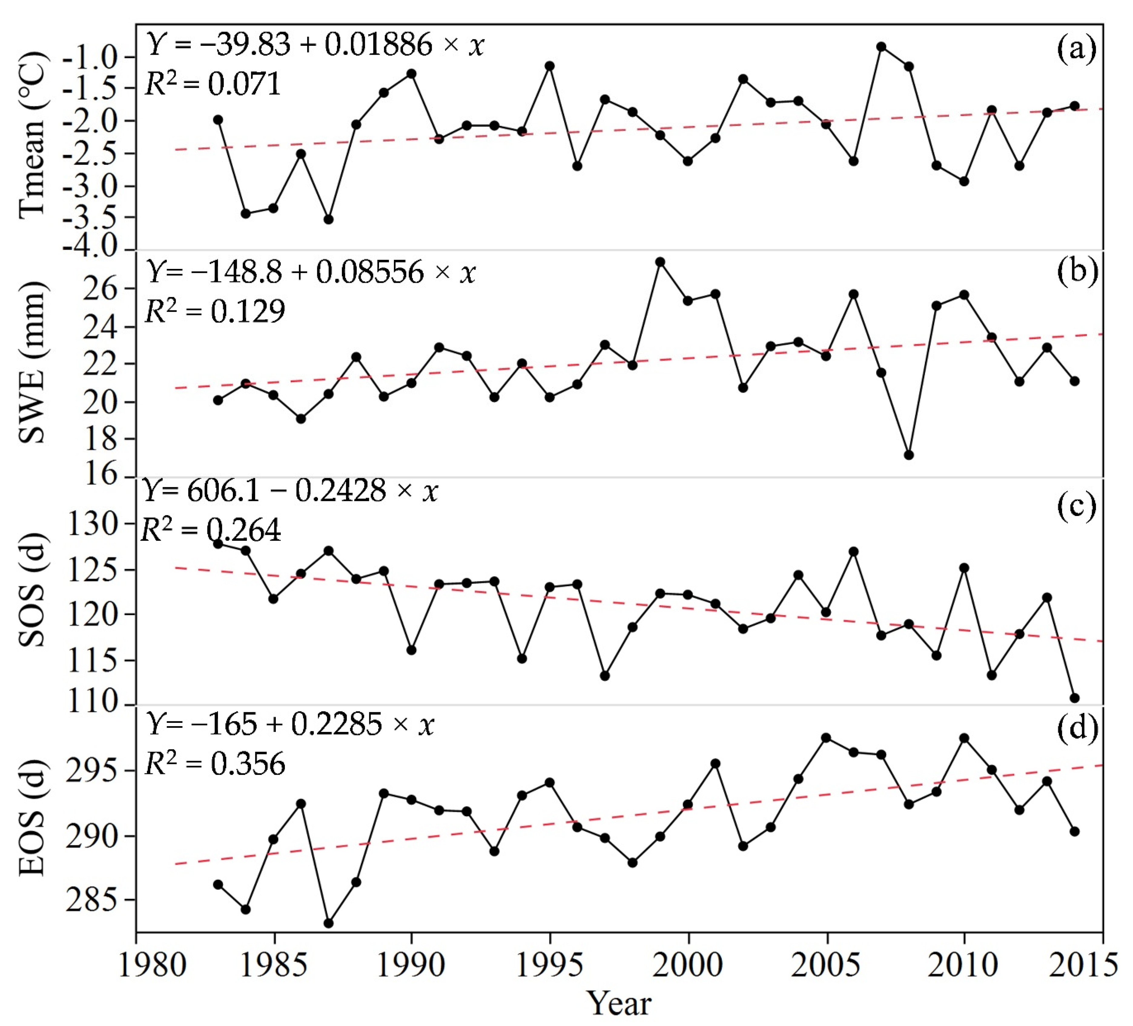
3.3. SOS and EOS Trends in Relation to Climate

Figure 5 illustrates the response of the SOS, as well as the EOS, in the forest ecosystem of the China–Mongolia–Russia International Economic Corridor to the monthly mean temperature and monthly snow water equivalent (SWE), according to PLS regression. The PLS regression analysis included both temperatures and SWE as important variables in an explanatory model for the SOS and EOS.
For the SOS, the variable importance plots (VIPs), as shown in Figure 5a,b indicate that the temperature in pre-year July, March, April and May, and the SWE in the winter half-year from November to the following April, play an essential role in determining the SOS in the forest ecosystem in our study area (VIP > 0.8). Temperatures in spring (March, April and May) have negative model coefficients, indicating that the warm temperature during these months advances the SOS. Temperatures in pre-year July have a positive model coefficient, indicating that the higher temperature may contribute to the delay of the SOS. It is clear that the temperature in April plays the dominant role in determining the SOS (MC = −0.86, VIP value = 2.45). We also calculated the relationship between SOS and Tmax and Tmin, which showed similar results, and no major difference was obtained. SWE in February and March has negative coefficients, suggesting that higher SWE in these months contributed to the advance of SOS, while the SWE in months such as November, December, January and April have positive model coefficients, indicating that the higher SWE in these months tends to delay the SOS.
Figure 5c,d illustrates the EOS responses to monthly temperature and SWE. Combining the model coefficients and VIP values, the temperature in months such as June, July, October and the pre-year December and the SWE in pre-year December and October determined the EOS. The high positive model coefficients in June, July and October indicate that the warmer temperature tends to delay the EOS, while the high negative model coefficient in pre-year December indicates that the temperature chilling is beneficial to the delaying of the EOS. The positive coefficient in pre-year December, March and April suggests that the higher SWE in these months tends to delay the EOS, while the negative coefficients in pre-year November, January and October indicate that the higher SWE might contribute to advances in EOS. PLS regression for different forest types was also conducted, but the results did not show significant differences.

4. Discussion

4.1. Trends and Spatiotemporal Variations in Forest Phenology

In this study, we investigated the start (SOS) and the end (EOS) date of the growing season in the forest ecosystem over the China–Mongolia–Russia International Economic Corridor by using long-term GIMMS NDVI records and the double logistic model from 1982 to 2015. The SOS and EOS of forests in our study area are 120.8 ± 7.8 and 290.9 ± 9.5 Julian days, respectively, and the spatial distribution pattern of these two phenological parameters is roughly consistent with two previous studies in mid- and high-latitudes in the Northern hemisphere [14,15].
Similar to numerous previous studies, our results showed a significant advance in the SOS with the background of climate warming [13,18]. We found that the average SOS of the forest ecosystem advanced at a rate of 2.5 days/decade in our study area. Myneni et al. (1997) reported that the SOS advanced by 8 ± 3 days from 1981 to 1991 in northern latitudes (45–70° N) [11]. Deng et al. (2019) found that the SOS in boreal forests varied with an average advancement rate of 3.38 days/decade [17]. The difference in trends is mainly attributed to the mismatch of the spatial extension and temporal duration. Even utilizing the same time series data, Jeong et al. (2011) found that the SOS advanced by 5.2 days from 1982–1999 but advanced by only 0.2 days from 2000–2008 in the Northern Hemisphere’s temperate vegetation [14]. It should also be noted that our study also detected a significant delay in the EOS, at a rate of 2.3 days/decade. Usually, the SOS is considered to be the most sensitive phenological parameter in response to global warming, while the EOS changes show more uncertainty [23]. Our results indicate that the EOS is as significant as the SOS in response to climate change and in determining the length of the growing season. Undeniably, however, the trends in the EOS appeared to be more spatially variable compared with those of the SOS, suggesting a more complicated feedback mechanism of the EOS to climate variation.

4.2. Relationship between SOS/EOS and Climatic Factors

The warming temperature triggering the advance of the SOS for diverse vegetation types has been widely reported [16,43]. Our results found that the SOS of the forest ecosystem in our study area was highly dependent on the temperature in April (MC = −0.86, VIP = 2.45). Though the PLS regression showed that the temperatures in other spring months, such as March and May, are also important variables in determining the advance of the SOS, their model coefficients are relatively small, indicating a relatively slight impact. Different to other studies, we chose the SWE instead of precipitation as a latent factor influencing forest phenology variations. Our results found that the winter SWE from pre-year November to current year April are essential factors in determining the SOS. The SOS is negative to SWE in February and March, while positive in other winter months. A greater snow depth can increase the amount of available water used for vegetation growth as well as maintain the soil temperature and nutrients [22]. Furthermore, the phenological changes in the boreal regions may be partially related to snowmelt timing variations [44,45]. Our results suggest that the higher SWE in February and March created adequate water, temperature and nutrient conditions for the forest green-up and the rapid increase in temperature accompanied by the decrease in snow water equivalent in April, which accelerated the advance of the SOS.
The autumn dormancy and the associated mechanisms in the forest are not well documented as compared with those of the SOS [23]. Our results found that the warmer summer is conducive to the extension of the growing season, which was consistent with most published studies [46,47]. Though the SOS showed different responses to monthly SWE, our results showed that the pre-year December and current year October SWE play a dominant role in determining the EOS. Previous studies showed that winter chilling has the potential to advance the SOS [48,49]. Our results suggest that the temperature chilling, as well as higher SWE in December, tend to have more potential to extend the EOS instead of the SOS. As the winter chilling requirements can always be sufficient in this mid–high region, the chilling environment and the snow cover protection may trigger more robust photosynthesis and a more extended photoperiod in the next growing season, as documented by Grippa et al. (2005) [24]. On the other hand, our study also suggested that using the annual values or preseason values to reveal the relationship between the SOS/EOS and its latent driving factors may be defective unless the response trends of these months are consistent between each other.

4.3. Uncertainties and Future Works

In this study, we estimated the forest phenology in the China–Mongolia–Russia International Economic Corridor, based on remote sensing observation records. By using the available in situ phenology observation data, we verified that the start and end dates of the growing season in Northeast China and the root mean square error of the simulated SOS and EOS are 3.14 and 3.90 days [41], indicating that the double logistic model and the threshold can detect the phenology effectively. Though our results showed a similar SOS and EOS pattern compared with previous studies [14,15], the in situ phenology observations in Mongolia and Russia are still further required to verify our results presented here.
It should be noted that, though the needleleaved evergreen forest shared similar average SOS and EOS values with other forest types, the standard deviations are much higher, suggesting that significant phenology uncertainties exist in the needleleaved evergreen forest. With evergreen leaves, the changes in the photosynthetic capacity and dormancy are hard to detect [50]. Wu et al. (2014) documented that widely used NDVI and EVI may exhibit limited potential in tracking growing season phenology, especially for the evergreen needleleaf forest ecosystems [39], which can explain why some needleleaved evergreen forest showed smaller SOS values (<110 days of Julian) in spring and larger values in autumn (>300 days in the autumn). A field-based survey, as well as a study of the temperature thresholds, should be further conducted to verify the accuracy of our results.
Furthermore, the boreal forests are vulnerable to global warming, which may contribute to the forest shift, and the increased fire or insect disturbances may change the forest pattern on the local scale [51]. Though we already eliminated the uncertainty caused by the land cover changes through using unchanged forest cover pixels based on the long-term land cover series (1992–2015), the lack of land use and land cover data before 1992 may result in some forest conversions due to human activities being ignored and, as a result, add to the uncertainty of our results.

5. Conclusions

In this study, the long-term changes in the forest phenology and the associated relationship with the temperatures and snow water equivalent over the China–Mongolia–Russia International Economic Corridor were examined by analyzing satellite-measured normalized difference vegetation index and meteorological observation data during 1982 to 2015. The average SOS of the forest ecosystem in our study area advanced at a rate of 2.5 days/decade, while the EOS was delayed at a rate of 2.3 days/decade, contributing to a growing season approximately 15 days longer in the 2010s compared to that in 1980s. A higher April temperature is beneficial to the advance in the SOS, and the higher summer temperature has the potential to extend the EOS in the forest ecosystem. However, our results also suggested that a single temperature cannot fully explain the advance of the SOS, as well as the delay in the EOS. The preseason SWE is also an essential factor in influencing the growing season. A higher SWE in February and March, and lower SWE in April, tend to advance the SOS, while higher SWE in pre-year December and lower SWE in current year October are beneficial to the extension of the EOS. Our results suggest both the temperature and snow water equivalent should be combined in predicting the forest phenology variations over China–Mongolia–Russia in the future. Furthermore, our findings would have further implications for reasonably estimating the productivity of the forest ecosystem and evaluating the regional ecosystem service value under the changing climate and economic development.

Author Contributions

Conceptualization, methodology and writing, L.Y.; climate data processing, Z.Y.; project administration and funding acquisition, S.Z. All authors have read and agreed to the published version of the manuscript.

Funding

This research was funded by National Natural Science Foundation of China, grant number, 41701493, the Scientific and Technological Development Program of Jilin province (20190103152JH), National Science and Technology basic Resources Survey Project of “Multidisciplinary Joint Scientific Expedition for China-Mongolia-Russia Economic Corridor”, grant number, 2017FY101301.

Acknowledgments

The authors want to thank the anonymous reviewers for their valuable and constructive comments/suggestions to help improve the paper.

Conflicts of Interest

The authors declare no conflict of interest.

References

  1. Menzel, A.; Fabian, P. Growing Season Extended in Europe. Nature 1999, 397, 659. [Google Scholar] [CrossRef]
  2. Stockli, R.; Vidale, P.L. European Plant Phenology and Climate as Seen in a 20-Year Avhrr Land-Surface Parameter Dataset. Int. J. Remote Sens. 2004, 25, 3303–3330. [Google Scholar] [CrossRef]
  3. Christiansen, D.E.; Markstrom, S.L.; Hay, L.E. Impacts of Climate Change on the Growing Season in the United States. Earth Interact. 2011, 15, 1–17. [Google Scholar] [CrossRef]
  4. Cook, K.H.; Vizy, E.K. Impact of Climate Change on Mid-Twenty-First Century Growing Seasons in Africa. Clim. Dyn. 2012, 39, 2937–2955. [Google Scholar] [CrossRef] [Green Version]
  5. Vujadinovic, M.; Vukovic, A.; Djurdjevic, V.; Rankovic-Vasic, Z.; Atanackovic, Z.; Sivcev, B.; Markovic, N.; Petrovic, N. Impact of Climate Change on Growing Season and Dormant Period Characteristics for the Balkan Region. Acta Hortic. 2012, 931, 87–94. [Google Scholar] [CrossRef]
  6. Bradley, N.L.; Leopold, A.C.; Ross, J.; Huffaker, W. Phenological Changes Reflect Climate Change in Wisconsin. Proc. Natl. Acad. Sci. USA 1999, 96, 9701–9704. [Google Scholar] [CrossRef] [Green Version]
  7. Euskirchen, E.S.; Mcguire, A.D.; Chapin, F.S. Energy Feedbacks of Northern High-Latitude Ecosystems to the Climate System Due to Reduced Snow Cover During 20th Century Warming. Glob. Chang. Biol. 2007, 13, 2425–2438. [Google Scholar] [CrossRef]
  8. Loarie, S.R.; Duffy, P.B.; Hamilton, H.; Asner, G.P.; Field, C.B.; Ackerly, D.D. The Velocity of Climate Change. Nature 2009, 462, 1052–1055. [Google Scholar] [CrossRef] [PubMed]
  9. Intergovernmental Panel on Climate Change. A Simple Method for Reconstructing a High-Quality Ndvi Time-Series Data Set Based on the Savitzky-Golay Filter. Remote Sens. Environ. 2013, 91, 332–344. [Google Scholar]
  10. Beerling, D.J.; Woodward, F.I. The Climate-Change Experiment (Climex)—Phenology and Gas-Exchange Responses of Boreal Vegetation to Global Change. Glob. Ecol. Biogeogr. Lett. 1994, 4, 17–26. [Google Scholar] [CrossRef]
  11. Myneni, R.B.; Keeling, C.D.; Tucker, C.J.; Asrar, G.; Nemani, R.R. Increased Plant Growth in the Northern High Latitudes from 1981 to 1991. Nature 1997, 386, 698–702. [Google Scholar] [CrossRef]
  12. White, M.A.; Thornton, P.E.; Running, S.W. A Continental Phenology Model for Monitoring Vegetation Responses to Interannual Climatic Variability. Glob. Biogeochem. Cycles 1997, 11, 217–234. [Google Scholar] [CrossRef]
  13. Piao, S.L.; Fang, J.Y.; Zhou, L.M.; Ciais, P.; Zhu, B. Variations in Satellite-Derived Phenology in China‘s Temperate Vegetation. Glob. Chang. Biol. 2006, 12, 672–685. [Google Scholar] [CrossRef]
  14. Jeong, S.J.; Ho, C.H.; Gim, H.J.; Brown, M.E. Phenology Shifts at Start Vs. End of Growing Season in Temperate Vegetation over the Northern Hemisphere for the Period 1982-2008. Glob. Chang. Biol. 2011, 17, 2385–2399. [Google Scholar] [CrossRef]
  15. Zhang, X.Y.; Friedl, M.A.; Schaaf, C.B.; Strahler, A.H. Climate Controls on Vegetation Phenological Patterns in Northern Mid- and High Latitudes Inferred from Modis Data. Glob. Chang. Biol. 2004, 10, 1133–1145. [Google Scholar] [CrossRef]
  16. Piao, S.L.; Tan, J.G.; Chen, A.P.; Fu, Y.H.; Ciais, P.; Liu, Q.; Janssens, I.A.; Vicca, S.; Zeng, Z.Z.; Jeong, S.J.; et al. Pennuelas. Leaf Onset in the Northern Hemisphere Triggered by Daytime Temperature. Nat. Commun. 2015, 6, 6911. [Google Scholar] [CrossRef] [Green Version]
  17. Deng, G.R.; Zhang, H.Y.; Guo, X.Y.; Shan, Y.; Ying, H.; Wu, R.H.; Li, H.; Han, Y.L. Asymmetric Effects of Daytime and Nighttime Warming on Boreal Forest Spring Phenology. Remote Sens. 2019, 11, 1651. [Google Scholar] [CrossRef] [Green Version]
  18. Yu, H.; Luedeling, E.; Xu, J. Winter and Spring Warming Result in Delayed Spring Phenology on the Tibetan Plateau. Proc. Natl. Acad. Sci. USA 2010, 107, 22151–22156. [Google Scholar] [CrossRef] [Green Version]
  19. Shen, M.; Piao, S.; Cong, N.; Zhang, G.; Jassens, I.A. Precipitation Impacts on Vegetation Spring Phenology on the Tibetan Plateau. Glob. Chang. Biol. 2015, 21, 3647–3656. [Google Scholar] [CrossRef] [Green Version]
  20. Shen, X.; Liu, B.; Henderson, M.; Wang, L.; Wu, Z.; Wu, H.; Jiang, M.; Lu, X. Asymmetric Effects of Daytime and Nighttime Warming on Spring Phenology in the Temperate Grasslands of China. Agric. For. Meteorol. 2018, 259, 240–249. [Google Scholar] [CrossRef]
  21. Groffman, P.M.; Driscoll, C.T.; Fahey, T.J.; Hardy, J.P.; Fitzhugh, R.D.; Tierney, G.L. Colder Soils in a Warmer World: A Snow Manipulation Study in a Northern Hardwood Forest Ecosystem. Biogeochemistry 2001, 56, 135–150. [Google Scholar] [CrossRef]
  22. Peng, S.; Piao, S.; Ciais, P.; Fang, J.; Wang, X. Change in Winter Snow Depth and Its Impacts on Vegetation in China. Glob. Chang. Biol. 2010, 16, 3004–3013. [Google Scholar] [CrossRef]
  23. Richardson, A.D.; Keenan, T.F.; Migliavacca, M.; Ryu, Y.; Sonnentag, O.; Toomey, M. Climate Change, Phenology, and Phenological Control of Vegetation Feedbacks to the Climate System. Agric. For. Meteorol. 2013, 169, 156–173. [Google Scholar] [CrossRef]
  24. Grippa, M.; Kergoat, L.; Le Toan, T.; Mognard, N.M.; Delbart, N.; L’Hermitte, J.; Vicente-Serrano, S.M. The Impact of Snow Depth and Snowmelt on the Vegetation Variability over Central Siberia. Geophys. Res. Lett. 2005, 32. [Google Scholar] [CrossRef]
  25. Belt and Road Initiative. Overview-Belt and Road Initiative Forum 2019; Belt and Road Forum for International Cooperation: Beijing, China, 2019. [Google Scholar]
  26. Yu, L.X.; Liu, T.X.; Zhang, S.W. Temporal and Spatial Changes in Snow Cover and the Corresponding Radiative Forcing Analysis in Siberia from the 1970s to the 2010s. Adv. Meteorol. 2017, 2017, 1–11. [Google Scholar] [CrossRef] [Green Version]
  27. European Space Agency. Land Cover Cci Product User Guide Version 2. Tech. Rep. Available online: Maps.Elie.Ucl.Ac.Be/Cci/Viewer/Download/Esacci-Lc-Ph2-Pugv2_2.0.Pdf (accessed on 25 March 2020).
  28. Tucker, C.; Pinzón, J.; Brown, M.E.; Slayback, D.; Pak, E.W.; Mahoney, R.; Vermote, E.; Saleous, N. An Extended Avhrr 8-Km Ndvi Dataset Compatible with Modis and Spot Vegetation Ndvi Data. Int. J. Remote.Sens. 2005, 26, 4485–4498. [Google Scholar] [CrossRef]
  29. Zhang, X.; Friedl, M.A.; Schaaf, C. Sensitivity of vegetation phenology detection to the temporal resolution of satellite data. Int. J. Remot. Sens. 2009, 30, 2061–2074. [Google Scholar] [CrossRef]
  30. Duveiller, G.; Hooker, J.; Cescatti, A. The mark of vegetation change on Earth’s surface energy balance. Nat. Commun. 2018, 9, 1–12. [Google Scholar] [CrossRef] [Green Version]
  31. Li, C.; Li, M.; Liu, J.; Li, Y.; Dai, Q.S. Comparative Analysis of Seasonal Landsat 8 Images for Forest Aboveground Biomass Estimation in a Subtropical Forest. Forests 2019, 11, 45. [Google Scholar] [CrossRef] [Green Version]
  32. Qiu, T.; Song, C.; Zhang, Y.; Liu, H.; Vose, J.M. Urbanization and climate change jointly shift land surface phenology in the northern mid-latitude large cities. Remote Sens. Environ. 2020, 236, 111477. [Google Scholar] [CrossRef]
  33. Liu, T.; Zhang, S.; Xu, X.; Bu, K.; Ning, J.; Chang, L. High resolution land cover datasets integration and application based on Landsat and Globcover data from 1975 to 2010 in Siberia. Chin. Geogr. Sci. 2016, 26, 429–438. [Google Scholar] [CrossRef] [Green Version]
  34. Liu, J.; Kuang, W.; Zhang, Z.; Xu, X.; Qin, Y.; Ning, J.; Zhou, W.; Zhang, S.; Li, R.; Yan, C.; et al. Spatiotemporal characteristics, patterns, and causes of land-use changes in China since the late 1980s. J. Geogr. Sci. 2014, 24, 195–210. [Google Scholar] [CrossRef]
  35. Harris, I.; Osborn, T.J.; Jones, P.; Lister, D. Version 4 of the CRU TS monthly high-resolution gridded multivariate climate dataset. Sci. Data 2020, 7, 109–118. [Google Scholar] [CrossRef] [PubMed] [Green Version]
  36. Luojus, K. European Space Agency (Esa) Globsnow Snow Water Equivalent (Swe) V2.0 L3b Monthly Data (1979–2013); Finnish Meteorological Institute: Helsinki, Finland, 2015.
  37. Zhang, X.; Friedl, M.A.; Schaaf, C.; Strahler, A.H.; Hodges, J.C.; Gao, F.; Reed, B.C.; Huete, A. Monitoring vegetation phenology using MODIS. Remote Sens. Environ. 2003, 84, 471–475. [Google Scholar] [CrossRef]
  38. Liang, L.; Schwartz, M.; Fei, S. Validating satellite phenology through intensive ground observation and landscape scaling in a mixed seasonal forest. Remote Sens. Environ. 2011, 115, 143–157. [Google Scholar] [CrossRef]
  39. Wu, C.; Gonsamo, A.; Gough, C.M.; Chen, J.M.; Xu, S. Modeling growing season phenology in North American forests using seasonal mean vegetation indices from MODIS. Remote Sens. Environ. 2014, 147, 79–88. [Google Scholar] [CrossRef]
  40. Beck, P.S.A.; Atzberger, C.; Høgda, K.A.; Johansen, B.; Skidmore, A. Improved monitoring of vegetation dynamics at very high latitudes: A new method using Modis Ndvi. Remote Sens. Environ. 2006, 100, 321–334. [Google Scholar] [CrossRef]
  41. Yu, L.; Liu, T.; Bu, K.; Yan, F.; Yang, J.; Chang, L.; Zhang, S. Monitoring the long term vegetation phenology change in Northeast China from 1982 to 2015. Sci. Rep. 2017, 7, 14770. [Google Scholar] [CrossRef] [Green Version]
  42. Wold, S.; Sjöström, M.; Eriksson, L. PLS-regression: A basic tool of chemometrics. Chemom. Intell. Lab. Syst. 2001, 58, 109–130. [Google Scholar] [CrossRef]
  43. Peng, S.; Piao, S.; Ciais, P.; Myneni, R.; Chen, A.; Chevallier, F.; Dolman, H.; Janssens, I.A.; Peñuelas, J.; Zhang, G.; et al. Asymmetric effects of daytime and night-time warming on Northern Hemisphere vegetation. Nature 2013, 501, 88–92. [Google Scholar] [CrossRef]
  44. Shabanov, N.; Zhou, L.; Knyazikhin, Y.; Myneni, R.; Tucker, C. Analysis of interannual changes in northern vegetation activity observed in AVHRR data from 1981 to 1994. IEEE Trans. Geosci. Remote Sens. 2002, 40, 115–130. [Google Scholar] [CrossRef] [Green Version]
  45. Dye, D.G.; Tucker, C.J. Seasonality and trends of snow-cover, vegetation index, and temperature in northern Eurasia. Geophys. Res. Lett. 2003, 30, 30. [Google Scholar] [CrossRef]
  46. Doi, H.; Takahashi, M. Latitudinal patterns in the phenological responses of leaf colouring and leaf fall to climate change in Japan. Glob. Ecol. Biogeogr. 2008, 17, 556–561. [Google Scholar] [CrossRef]
  47. Estrella, N.; Menzel, A. Responses of leaf colouring in four deciduous tree species to climate and weather in Germany. Clim. Res. 2006, 32, 253–267. [Google Scholar] [CrossRef] [Green Version]
  48. Zhang, X.; Tarpley, D.; Sullivan, J.T. Diverse responses of vegetation phenology to a warming climate. Geophys. Res. Lett. 2007, 34, 34. [Google Scholar] [CrossRef]
  49. Migliavacca, M.; Sonnentag, O.; Keenan, T.F.; Cescatti, A.; O’Keefe, J.; Richardson, A.D.; O’keefe, J. On the uncertainty of phenological responses to climate change, and implications for a terrestrial biosphere model. Biogeosciences 2012, 9, 2063–2083. [Google Scholar] [CrossRef] [Green Version]
  50. Nichol, C.J.; Lloyd, J.; Shibistova, O.; Arneth, A.; Roser, C.; Knohl, A.; Matsubara, S.; Grace, J. Remote Sensing of Photosynthetic-Light-Use Efficiency of a Siberian Boreal Forest. Tellus Ser. B-Chem. Phys. Meteorol. 2002, 54, 677–687. [Google Scholar] [CrossRef]
  51. Bonan, G.B. Forests and Climate Change: Forcings, Feedbacks, and the Climate Benefits of Forests. Science 2008, 320, 1444–1449. [Google Scholar] [CrossRef] [PubMed] [Green Version]
Figure 1. The spatial distribution of the main land cover types in the China–Mongolia–Russia International Economic Corridor.
Forests 11 00757 g001
Figure 2. Spatial distribution of start date of the growing season (SOS, a) and the end date of the season (EOS, b) in the China–Mongolia–Russia International Economic Corridor.
Forests 11 00757 g002
Figure 3. Spatial distribution of change trend in start date of the growing season (SOS, a) and end date of the growing season (EOS, b) from 1982 to 2015 in the China–Mongolia–Russia International Economic Corridor. The bottom left inset shows the pixels with significant (p < 0.1, p < 0.05 and p < 0.01) SOS or EOS change.
Forests 11 00757 g003
Figure 4. Trends and temporal variations of annual mean temperature (a), annual mean snow water equivalent (b), SOS (c) and EOS (d) for forest vegetation in the China–Mongolia–Russia International Economic Corridor between 1983 and 2014.
Forests 11 00757 g004
Figure 5. Responses of SOS and EOS in forest vegetation of the China–Mongolia–Russia International Economic Corridor to monthly temperatures (a,c) and monthly SWE (b,d) according to PLS regression.
Forests 11 00757 g005
Table 1. The mean and standard deviation of start date (SOS) and the end date (EOS) of the growing season for different forests types.
IDForest TypeCountArea
(104 km2)
SOS
(mean)
SOS
(std)
EOS
(mean)
EOS
(std)
1Broadleaved deciduous forest16,996118.03120.675.28291.959.07
2Needleleaved evergreen forest969567.33119.7311.08290.758.94
3Needleleaved deciduous forest26,068181.03121.817.53291.229.86
4Mixed forest508035.28120.028.25288.079.08

