Estimating Urban Vegetation Biomass from Sentinel-2A Image Data


Abstract
1. Introduction
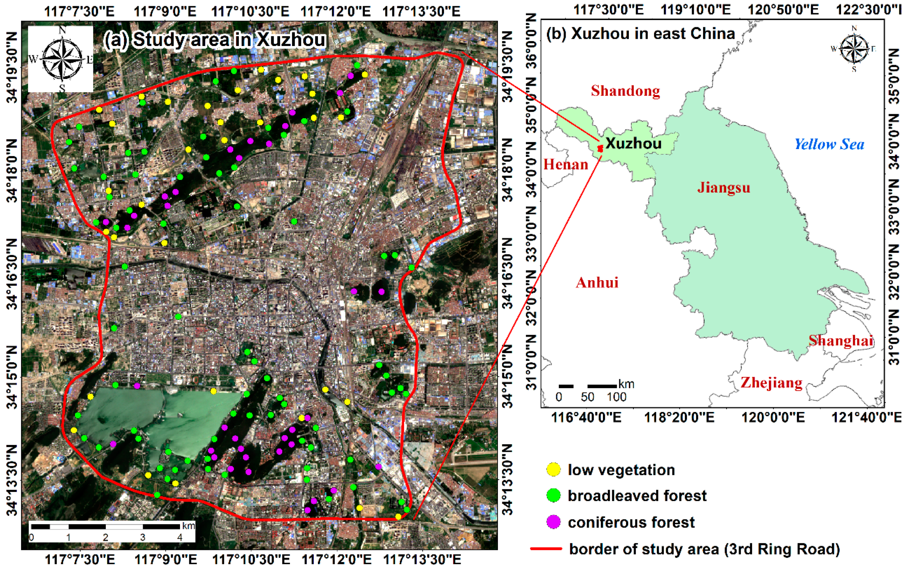
2. Study Area
3. Materials and Methods
3.1. Remote Sensing Data
3.2. Urban Vegetation Classification
3.3. Candidate Variables for Modeling
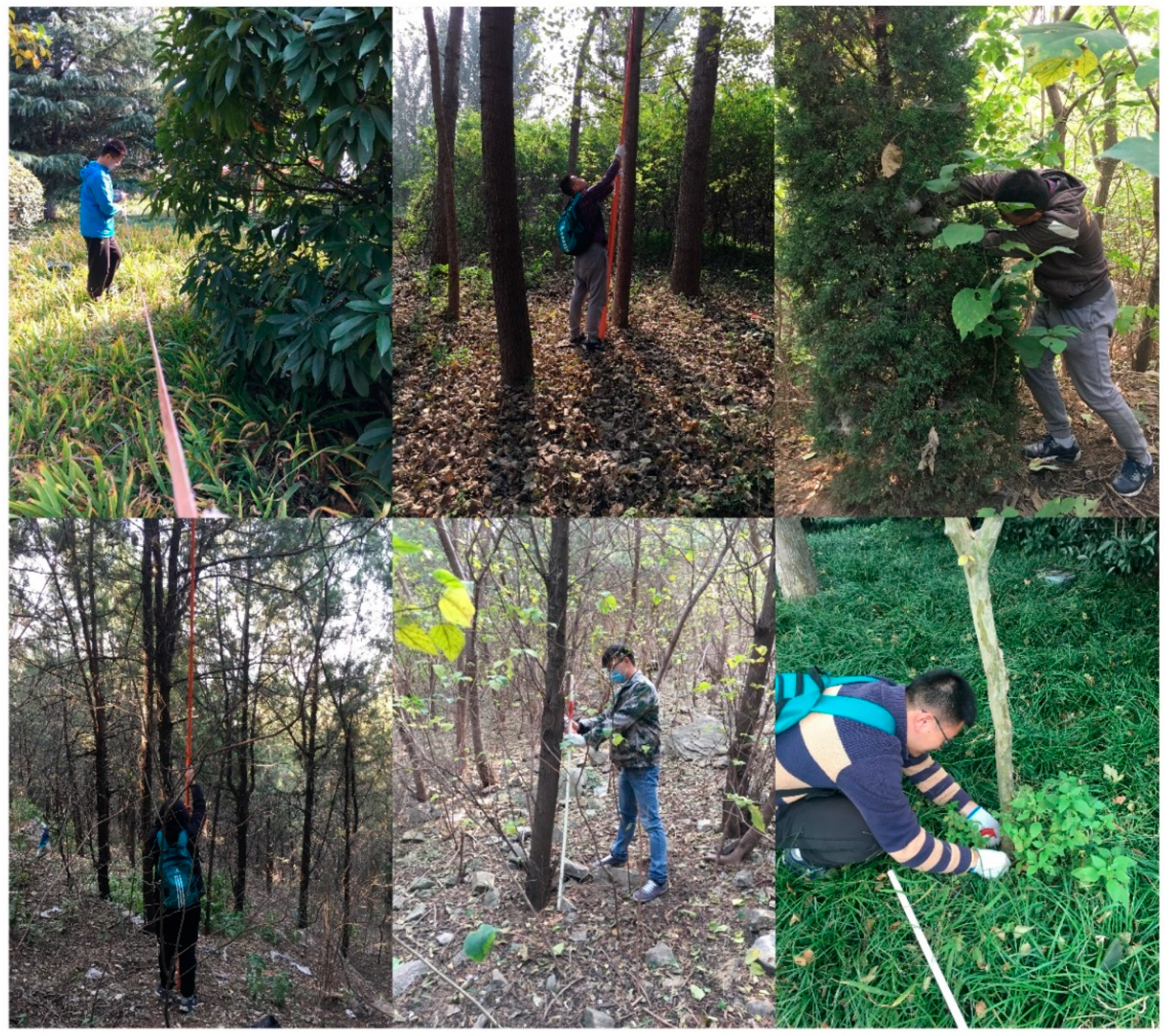
3.4. Field Measurements
3.5. Modeling
3.5.1. Correlation Analysis
3.5.2. Stepwise Regression Modeling
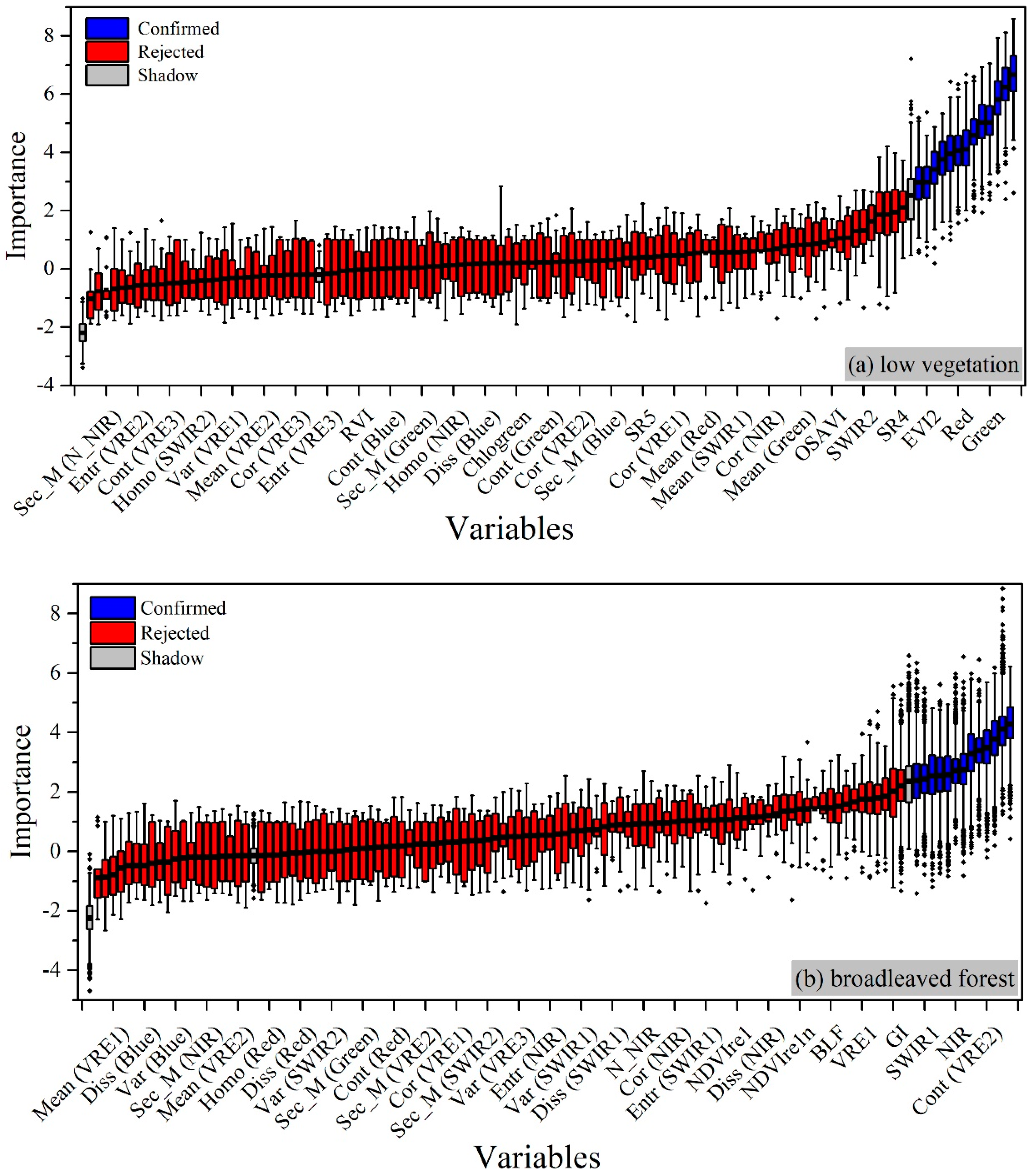
3.5.3. Boruta Based Multiple Linear Regression Modeling
3.5.4. Accuracy Assessment
3.6. Seasonal Variation of Urban Vegetation Biomass
4. Results and Analysis
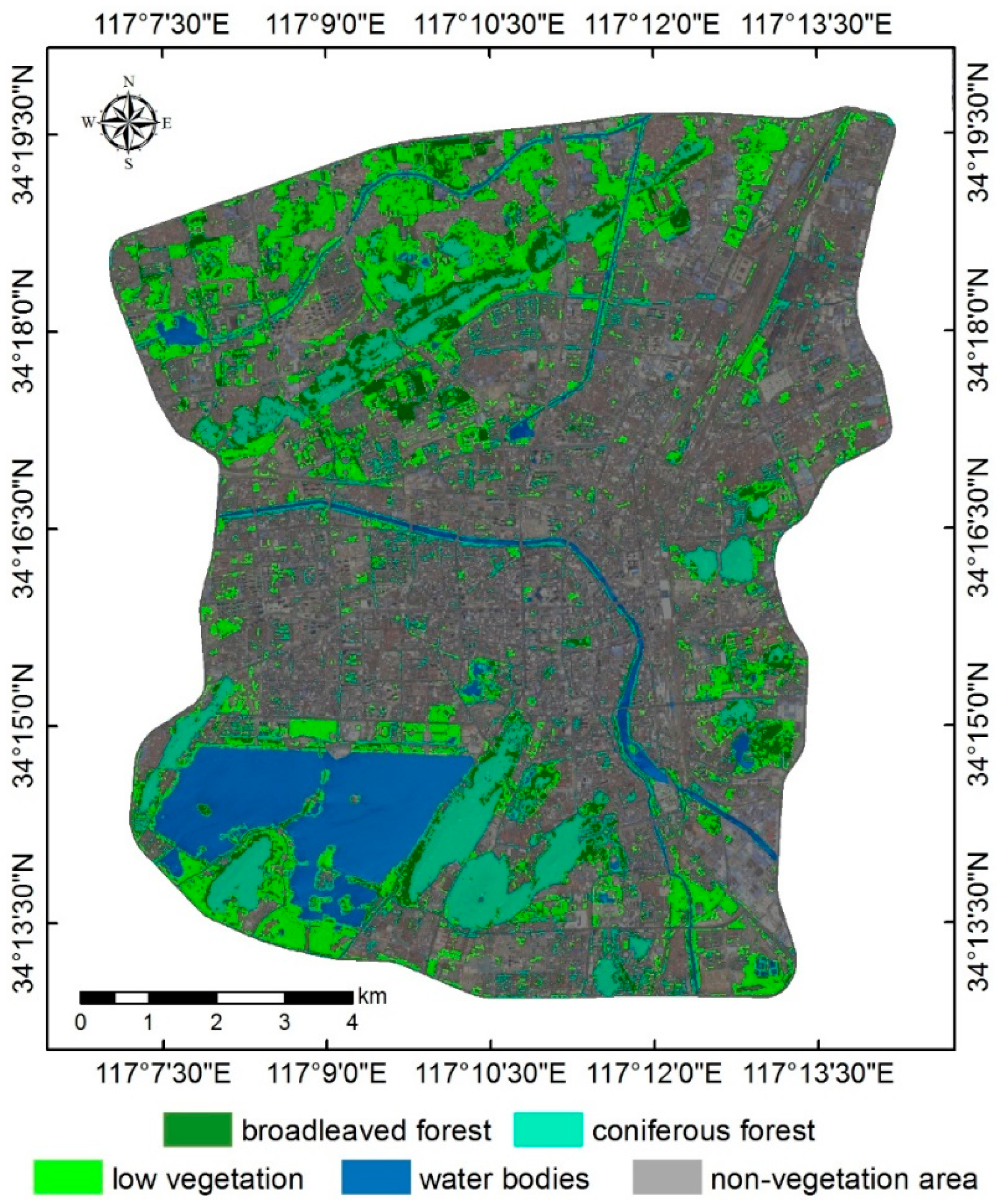
4.1. Urban Vegetation Classification
4.2. Correlations between Candidate Variables and Urban Vegetation Biomass
4.2.1. For Low Vegetation
4.2.2. For Broadleaved Forest
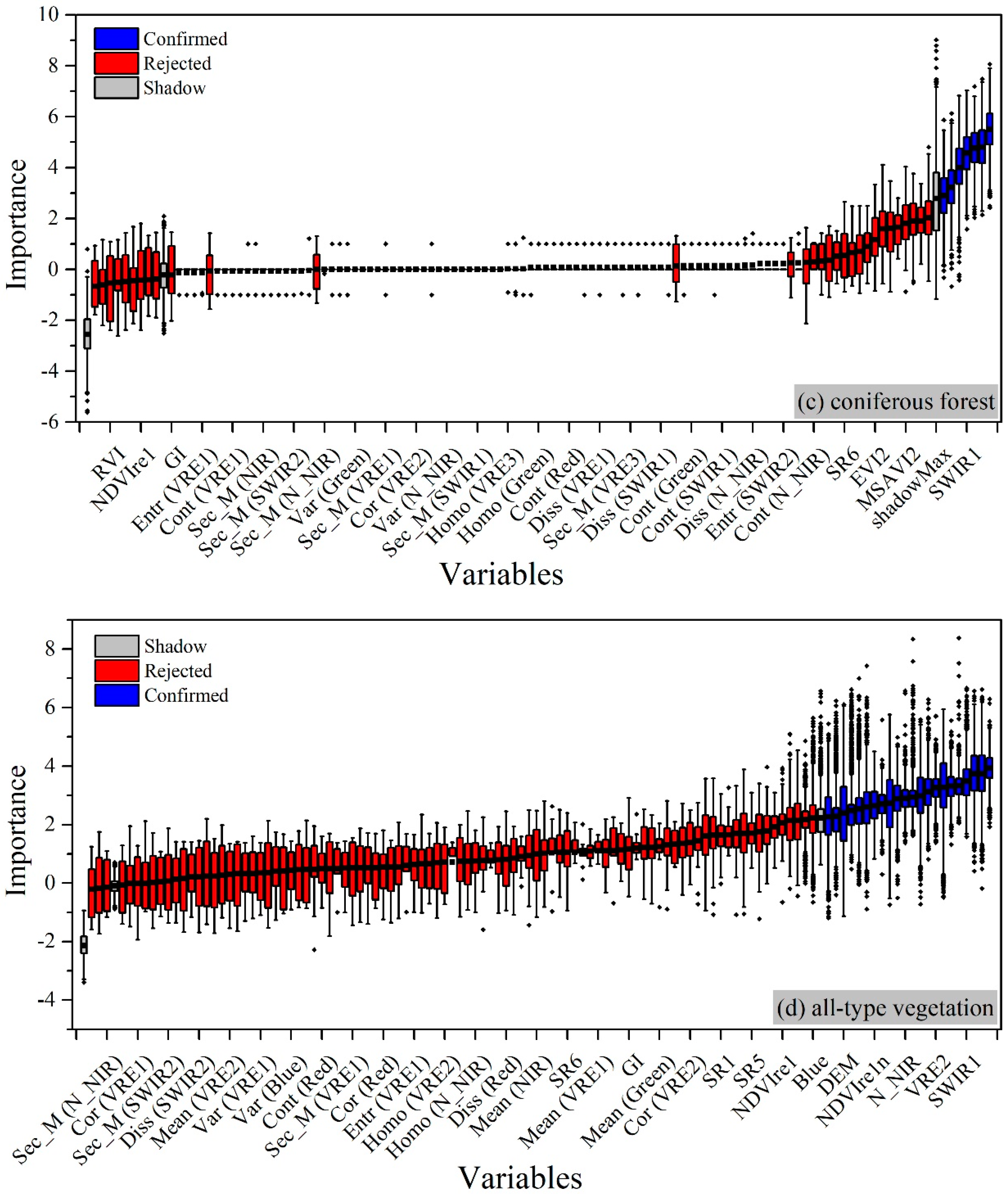
4.2.3. For Coniferous Forest
4.2.4. For All-Type Vegetation
4.3. Urban Vegetation Biomass Estimation Models
4.3.1. Stepwise Regression Models
4.3.2. Multiple Linear Regression Models
4.3.3. Accuracy Assessment
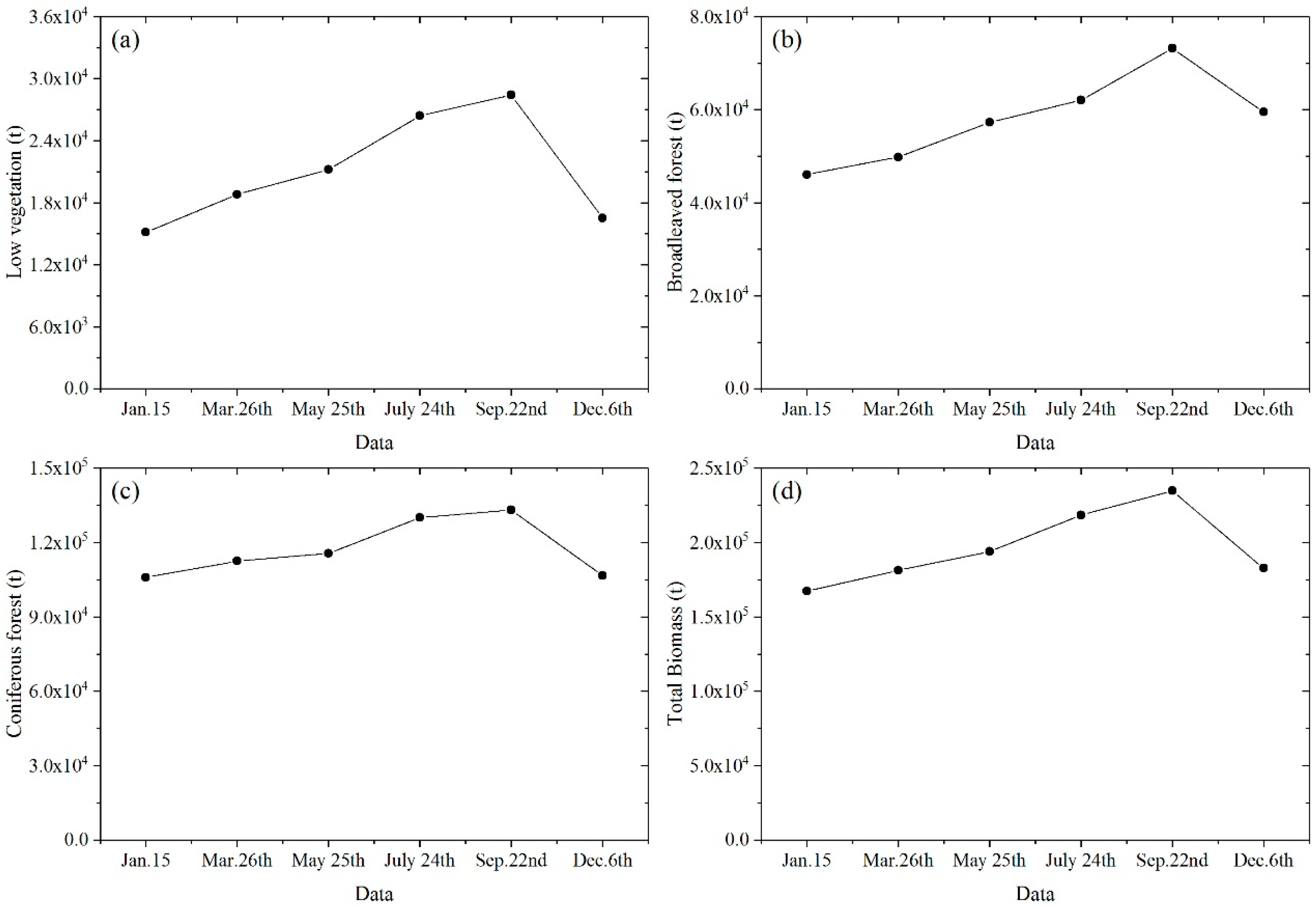
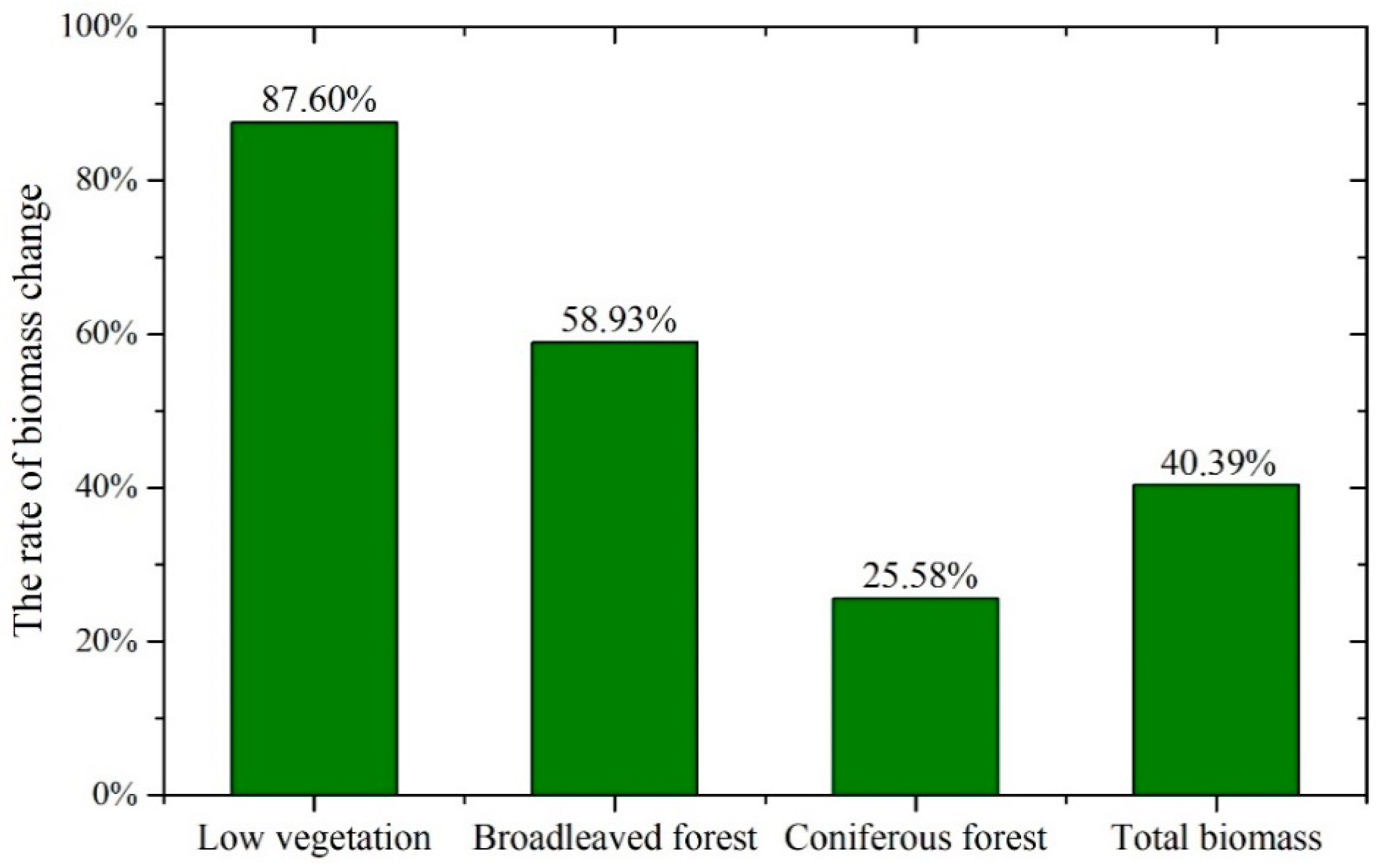
4.4. Seasonal Variation
5. Discussion
6. Conclusions
- Freely available multispectral Sentinel-2A satellite data has proven its capability in urban vegetation biomass estimation. The measured biomass of each vegetation type is closely correlated with different remote sensing derived variables, mostly spectral reflectance for low vegetation and coniferous forest and mostly textural features for broadleaved forest.
- The vegetation biomass estimation models built by the stepwise regression (SR) outperform those with the multiple linear regression. It is necessary to discriminate vegetation types in biomass modeling and the highest accuracy is obtained by the SR model for coniferous forest.
- Highest vegetation biomass occurs in autumn (September) while lowest in winter (January and December). Low vegetation and broadleaved forest have larger seasonal change rates than coniferous forest that consists mostly of evergreen trees.
Author Contributions
Funding
Acknowledgments
Conflicts of Interest
Appendix A

| Spectral Index | Formula |
|---|---|
| Green index (GI) | |
| Green normalized different vegetation index (gNDVI) | |
| Normalized difference vegetation index (NDVI) | |
| Ratio vegetation index (RVI) | |
| Difference vegetation index (DVI) | |
| Enhanced vegetation index 2 (EVI2) | |
| Chlorophyll green index (Chlogreen) | |
| Normalized difference vegetation index (NDVIre1) | |
| Normalized difference vegetation index (NDVIre1n) | |
| Simple ratio 1 (SR1) | |
| Simple ratio 2 (SR2) | |
| Simple ratio 3 (SR3) | |
| Simple ratio 4 (SR4) | |
| Simple ratio 5 (SR5) | |
| Simple ratio 6 (SR6) | |
| Simple ratio 7 (SR7) | |
| Normalized difference infrared index (NDII) | |
| Soil-adjusted vegetation index (SAVI) | |
| Modified soil-adjusted vegetation index 2 (MSAVI2) | |
| Optimized soil-adjusted vegetation index (OSAVI) |
| Tree species | Model | R2 | Reference |
|---|---|---|---|
| Platycladus orientalis | WS = 0.0573 (D2H) 0.8657 | 0.97 | [71] |
| WB = 0.0043 (D2H) 1.1085 | 0.89 | ||
| WL = 0.0038 (D2H) 1.0385 | 0.84 | ||
| WR = 0.0485 (D2H) 0.6886 | 0.80 | ||
| Robinia pseudoacacia | WS = 0.0681 (D2H) 0.9865 | 0.9545 | [72] |
| WB = 12020 + 0.009 (D2H) | 0.8862 | ||
| WL = −0.549 + 0.007 (D2H) | 0.9174 | ||
| WR = 0.0087 (D2H) 1.0513 | 0.9472 | ||
| Metasequoia glyptostroboides | WS = 0.0146 (D2H) 0.9835 | 0.993 | [73] |
| WB = 0.0243 (D2H) 0.7359 | 0.993 | ||
| WL = 0.0949 (D2H) 0.4795 | 0.982 | ||
| WR = 0.0102 (D2H) 0.8745 | 0.975 | ||
| Populus euramevicana | WS = 0.006 (D2H) 1.098 | 0.995 | [74] |
| WB =0.001 (D2H) 1.157 | 0.984 | ||
| WL = 0.012 (D2H) 0.685 | 0.955 | ||
| WR = 0.083 (D2H) 0.636 | 0.915 | ||
| Cinnamomum camphora | WS = 0.0914 (D2H) 0.7755 | 0.944 | [73] |
| WB = 0.0099 (D2H) 1.0256 | 0.946 | ||
| WL = 0.0011 (D2H) 1.1713 | 0.941 | ||
| WR = 0.0298 (D2H) 0.8740 | 0.935 | ||
| Ginkgo biloba | lnWS = −3.84 + 0.95ln (D2H) | 0.98 | [75] |
| lnWB = −9.38 + 1.46ln (D2H) | 0.852 | ||
| lnWL = −6.95 + 1.03ln (D2H) | 0.853 | ||
| lnWR = −5.60 + 1.07ln (D2H) | 0.967 | ||
| Platanus acerifolia | WT = 0.0690(D2H) 0.9133 | / | [76] |
| Larix gmelinii | lnWS = −2.8319 + 0.8379ln (D2H) | 0.9996 | [77] |
| lnWB = −3.9021 + 0.8822ln (D2H) | 0.9015 | ||
| lnWL = −4.0174 + 0.7659ln (D2H) | 0.9007 | ||
| lnWR = −3.6497 + 0.8247ln (D2H) | 0.9994 | ||
| Broussonetia papyrifera | WT = 0.07112 (D2H) 0.910358078 | / | [78] |
| Ligustrum lucidum | WS = 0.03939 (D2H) 0.95679 | 0.97 | [79] |
| WB = 0.03357 (D2H) 0.77809 | 0.84 | ||
| WL = 0.11613 (D2H) 0.45871 | 0.61 | ||
| WT = 0.11394 (D2H) 0.84957 | 0.97 | ||
| Koelreuteria bipinnata | WS = 0.08259 (D2H) 0.80831 | 0.97 | [79] |
| WB = 0.00053 (D2H) 1.29104 | 0.94 | ||
| WL = 0.01286 (D2H) 0.69408 | 0.81 | ||
| WT = 0.12238 (D2H) 0.84468 | 0.98 | ||
| Magnolia grandiflora | WS = 0.0649 (D2H) 0.8131 | 0.969 | [73] |
| WB = 0.0431 (D2H) 0.6697 | 0.904 | ||
| WL = 0.0254 (D2H) 0.8701 | 0.837 | ||
| WR = 0.0885 (D2H) 0.6713 | 0.883 | ||
| Liriodendron chinense | WS = 0.02426 (D2H) 0.942303 | 0.99537 | [80] |
| WB = 0.000349 (D2H) 1.268207 | 0.962865 | ||
| WL = 0.000419 (D2H) 1.048786 | 0.834806 | ||
| WR = 0.023475 (D2H) 0.770233 | 0.918072 | ||
| Paulownia fortunei | WS = 0.021158D 2.43244 | 0.9978 | [81] |
| WB = 0.057869D 2.06599 | 0.9959 | ||
| WL = 0.060045D 1.54688 | 0.9891 | ||
| WR = 0.030740D 2.10612 | 0.8387 |
| Species | Model | R2 | Species | Model | R2 |
|---|---|---|---|---|---|
| Ligustrum quihoui | WB = 26.332 (CH) 0.666 | 0.950 | Buxus bodinieri | WB = 262.879 (CH) 1.546 | 0.895 |
| WL = 14.646C 1.164 | 0.972 | WL = 224.662 (CH) 1.364 | 0.890 | ||
| WR = 18.721 (VC) 0.421 | 0.965 | WR = 294.262 (CH) 1.639 | 0.889 | ||
| WT = 52.388 (CH) 0.654 | 0.959 | WT = 756.343 (CH) 1.497 | 0.913 | ||
| Berberis thunbergii | WB = 73.468 (AC) 0.766 | 0.927 | Buxus megistophylla | WB = 15.572D 1.325 | 0.979 |
| WL = 3.340 (AC) 0.465 | 0.601 | WL = 20.649 + 9.047ln (CH) | 0.902 | ||
| WR = 29.029 (AC) 0.721 | 0.785 | WR = 9.654D 1.308 | 0.975 | ||
| WT = 104.637 (AC) 0.734 | 0.903 | WT = 35.982D 1.212 | 0.980 | ||
| Photinia serrulata | WB = 0.310 (D2H) 1.097 | 0.985 | Pittosporum tobira | WB = 765.073 (VC) 0.824 | 0.991 |
| WL = 0.264 (D2H) 0.916 | 0.986 | WL = 2.958 (D2H) 0.607 | 0.911 | ||
| WR = 0.259 (D2H) 1.053 | 0.988 | WR = 445.103 (VC) 0.742 | 0.972 | ||
| WT = 0.805 (D2H) 1.051 | 0.988 | WT = 1411.387 (VC) 0.742 | 0.979 | ||
| Hibiscus syriacus | WB = 108.688 (VC) 1.693 | 0.984 | Nandina domestica | WB = 75.700 (CH) 1.110 | 0.980 |
| WL = 18.925 (CH) 1.565 | 0.969 | WL = 11.109 + 17.911lnH | 0.971 | ||
| WR = 69.564 (VC) 1.563 | 0.985 | WR = 57.553 (CH) 1.187 | 0.939 | ||
| WT = 206.627 (VC) 1.589 | 0.986 | WT = 167.114 (CH) 1.174 | 0.960 | ||
| Lagerstroemia indica | WB = 30.213H 6.318 | 0.987 | Syringa oblata | WB = 0.876 (D2H) 0.894 | 0.988 |
| WL = 6.656H 5.065 | 0.994 | WL = 0.683 (D2H) 0.715 | 0.988 | ||
| WR = 20.934H 5.905 | 0.989 | WR = 0.603 (D2H) 0.877 | 0.991 | ||
| WT = 58.305H 6.065 | 0.989 | WT = 2.011 (D2H) 0.863 | 0.991 | ||
| Forsythia suspensa | WB = 0.385 (D2H) 1.025 | 0.997 | |||
| WL = 0.187 (D2H) 0.868 | 0.985 | ||||
| WR = 0.176 (D2H) 0.954 | 0.990 | ||||
| WT = 0.716 (D2H) 0.989 | 0.996 | ||||
| ID | Biomass (kg) | ID | Biomass (kg) | ID | Biomass (kg) | ID | Biomass (kg) |
|---|---|---|---|---|---|---|---|
| 1 | 1005.74 | 2 | 654.00 | 3 | 1192.37 | 5 | 1372.71 |
| 6 | 1711.81 | 7 | 11,250.00 | 8 | 972.12 | 9 | 1286.95 |
| 10 | 2118.96 | 11 | 1043.43 | 13 | 1258.78 | 14 | 1114.78 |
| 15 | 502.87 | 16 | 431.85 | 17 | 638.50 | 21 | 985.40 |
| 22 | 918.67 | 23 | 989.10 | 24 | 1212.90 | 25 | 349.37 |
| 26 | 732.72 | 27 | 838.38 | 28 | 1580.27 | 29 | 383.54 |
| 30 | 110.76 | 31 | 100.03 | 33 | 766.57 | 34 | 1556.81 |
| 35 | 917.00 | 36 | 56.07 | 37 | 383.64 | 38 | 1171.94 |
| 39 | 759.66 | 40 | 519.31 | 41 | 1383.84 | 42 | 1300.94 |
| 43 | 711.91 | 45 | 1158.74 | 46 | 831.58 | 47 | 447.30 |
| 48 | 906.36 | 50 | 607.56 | 51 | 362.14 | 52 | 325.44 |
| 53 | 734.24 | 54 | 634.06 | 55 | 2152.83 | 56 | 965.29 |
| 59 | 240.68 | 60 | 777.64 | 63 | 2042.87 | 65 | 1237.21 |
| 66 | 1573.60 | 67 | 901.01 | 68 | 1641.06 | 69 | 805.89 |
| 70 | 612.32 | 71 | 1658.79 | 72 | 433.56 | 74 | 2225.07 |
| 75 | 257.17 | 76 | 893.24 | 77 | 1209.58 | 80 | 8.23 |
| 82 | 706.14 | 83 | 989.41 | 84 | 1105.56 | 86 | 551.12 |
| 87 | 38.43 | 88 | 222.73 | 90 | 879.47 | 91 | 1285.60 |
| 92 | 17.95 | 94 | 442.08 | 95 | 822.52 | 96 | 680.24 |
| 97 | 1085.41 | 99 | 1153.80 | 100 | 188.35 | 101 | 11,085.08 |
| 106 | 2771.95 | 107 | 590.58 | 110 | 884.22 | 111 | 1531.30 |
| 116 | 984.55 | 117 | 3452.27 | 118 | 525.76 | 119 | 120.16 |
| 121 | 371.84 | 123 | 663.12 | 124 | 559.32 | 126 | 1610.53 |
| 127 | 866.05 | 129 | 3437.13 | 132 | 384.20 | 134 | 2179.22 |
| 135 | 216.23 | 137 | 2915.05 | 139 | 610.32 | 140 | 6.19 |
| 142 | 1100.06 | 143 | 1634.99 | 145 | 973.77 | 146 | 364.50 |
| 147 | 1421.20 | 148 | 1841.15 | 149 | 2707.82 | 151 | 969.84 |
| 152 | 2899.26 | 153 | 6.19 | 154 | 1176.14 | 156 | 1100.67 |
| 157 | 3279.12 | 158 | 6.19 | 159 | 1265.47 | 162 | 1007.43 |
| 163 | 2240.88 | 164 | 1189.30 | 166 | 6.19 | 168 | 6.19 |
| 169 | 6.19 | 170 | 698.32 | 172 | 198.72 | 173 | 6.19 |
| 174 | 1772.22 | 175 | 2304.31 | 176 | 6.19 | 177 | 6.19 |
| 178 | 1045.89 | 179 | 131.80 | 180 | 78.79 | 181 | 888.34 |
| 182 | 64.71 | 183 | 320.74 | 185 | 210.05 | 187 | 724.18 |
| 188 | 308.44 | 189 | 1002.98 | 190 | 6.19 | 192 | 623.21 |
| Vegetation Type | Rnh2 | Adj-Rnh2 | Variable | Coefficient | VIF |
|---|---|---|---|---|---|
| Low vegetation | 0.853 | 0.818 | Constant | −171.896 | |
| Low | −49.335 | 1.382 | |||
| CLF | 76.406 | 3.254 | |||
| gNDVI | 316.404 | 3.181 | |||
| SR2 | −13.710 | 4.274 | |||
| Cor (VRE2) | −0.365 | 1.311 | |||
| DEM | 1.087 | 1.207 | |||
| Broadleaved forest | 0.821 | 0.805 | Constant | 660.327 | |
| Cor (VRE2) | −16.739 | 2.095 | |||
| Green | −3601.606 | 1.066 | |||
| Cor (SWIR1) | 9.944 | 2.317 | |||
| OSAVI | −695.210 | 1.375 | |||
| Var (VRE2) | −196.861 | 5.043 | |||
| Cont (SWIR1) | 98.126 | 5.674 | |||
| Coniferous forest | 0.838 | 0.810 | Constant | 183.909 | |
| SWIR1 | −473.034 | 1.151 | |||
| SR3 | −0.016 | 1.346 | |||
| DEM | −0.232 | 1.109 | |||
| GI | 0.299 | 1.461 | |||
| Cor (VRE2) | 14.747 | 1.079 | |||
| All vegetation | 0.754 | 0.721 | Constant | 213.811 | |
| Green | −4566.311 | 4.279 | |||
| Cor (VRE2) | −5.370 | 1.889 | |||
| Red | 2655.001 | 4.530 | |||
| Cont (SWIR2) | 237.815 | 9.833 | |||
| Cont (VRE1) | −108.805 | 6.695 | |||
| Cor (N_NIR) | 0.366 | 1.905 | |||
| Var (SWIR1) | −273.149 | 3.947 | |||
| Var (Blue) | −395.915 | 3.295 | |||
| Var (VRE1) | 157.094 | 4.905 | |||
| Cont (Red) | −49.701 | 3.396 | |||
| Entr (Green) | 163.695 | 9.353 | |||
| Sec_M (VRE2) | −203.368 | 4.150 |
References
- United Nations. World Urbanization Prospects: The 2080 Revision; United Nations: New York, NY, USA, 2018. [Google Scholar]
- Zhou, X.; Li, L.; Chen, L.; Liu, Y.; Cui, Y.; Zhang, Y.; Zhang, T. Discriminating urban forest types from Sentinel-2A image data through linear spectral mixture analysis: A case study of Xuzhou, East China. Forests 2019, 10, 478. [Google Scholar] [CrossRef]
- Miller, R.W.; Hauer, R.J.; Werner, L.P. Urban Forestry: Planning and Managing Urban Greenspaces, 3rd ed.; Waveland Press, Inc.: Long Grove, IL, USA, 2015; ISBN 9781478606376. [Google Scholar]
- Zhao, S.; Tang, Y.; Chen, A. Carbon storage and sequestration of urban street trees in Beijing, China. Front. Ecol. Evol. 2016, 4, 53. [Google Scholar] [CrossRef]
- Cohen-Cline, H.; Turkheimer, E.; Duncan, G.E. Access to green space, physical activity and mental health: A twin study. J. Epidemiol. Community Health 2015, 69, 523–529. [Google Scholar] [CrossRef] [PubMed]
- White, M.P.; Alcock, I.; Wheeler, B.W.; Depledge, M.H. Would you be happier living in a greener urban area? A fixed-effects analysis of Panel Data. Psychol. Sci. 2013, 24, 920–928. [Google Scholar] [CrossRef] [PubMed]
- Wilkes, P.; Disney, M.; Vicari, M.B.; Calders, K.; Burt, A. Estimating urban above ground biomass with multi-scale LiDAR. Carbon Balance Manag. 2018, 13, 10. [Google Scholar] [CrossRef]
- Reis, C.; Lopes, A. Evaluating the cooling potential of urban green spaces to tackle urban climate change in Lisbon. Sustainability 2019, 11, 2480. [Google Scholar] [CrossRef]
- Pérez, G.; Perini, K. (Eds.) Nature Based Strategies for Urban and Building Sustainability; Elsevier: Oxford, UK, 2018; ISBN 9780128121504. [Google Scholar]
- He, M.; Zhao, B.; Ouyang, Z.; Yan, Y.; Li, B. Linear spectral mixture analysis of Landsat TM data for monitoring invasive exotic plants in estuarine wetlands. Int. J. Remote Sens. 2010, 31, 4319–4333. [Google Scholar] [CrossRef]
- He, H.; Zhang, C.; Zhao, X.; Fousseni, F.; Wang, J.; Dai, H.; Yang, S.; Zuo, Q. Allometric biomass equations for 12 tree species in coniferous and broadleaved mixed forests, Northeastern China. PLoS ONE 2018, 13, e0186226. [Google Scholar] [CrossRef]
- Weaver, T.; Collins, D. Measuring vegetation biomass and production. Am. Biol. Teach. 1988, 50, 164–166. [Google Scholar] [CrossRef]
- Launchbaugh, K. Direct Measures of Biomass. Available online: https://www.webpages.uidaho.edu/veg_measure/Modules/Lessons/Module7(Biomass&Utilization)/7_3_DirectMethods.htm (accessed on 1 October 2019).
- Wu, J. Developing general equations for urban tree biomass estimation with high-resolution satellite imagery. Sustainability 2019, 11, 4347. [Google Scholar] [CrossRef]
- Galidaki, G.; Zianis, D.; Gitas, I.; Radoglou, K.; Karathanassi, V.; Tsakiri-Strati, M.; Woodhouse, I.; Mallinis, G. Vegetation biomass estimation with remote sensing: Focus on forest and other wooded land over the Mediterranean ecosystem. Int. J. Remote Sens. 2017, 38, 1940–1966. [Google Scholar] [CrossRef]
- Lu, D. The potential and challenge of remote sensing-based biomass estimation. Int. J. Remote Sens. 2006, 27, 1297–1328. [Google Scholar] [CrossRef]
- Kumar, L.; Mutanga, O. Remote sensing of above-ground biomass. Remote Sens. 2017, 9, 935. [Google Scholar] [CrossRef]
- Sousa, A.M.O.; Gonçalves, A.C.; Mesquita, P.; Marques da Silva, J.R. Biomass estimation with high resolution satellite images: A case study of Quercus rotundifolia. ISPRS J. Photogramm. Remote Sens. 2015, 101, 69–79. [Google Scholar] [CrossRef]
- Simonson, W.; Ruiz-Benito, P.; Valladares, F.; Coomes, D. Modelling above-ground carbon dynamics using multi-temporal airborne lidar: Insights from a Mediterranean woodland. Biogeosciences 2016, 13, 961–973. [Google Scholar] [CrossRef]
- Gonzalez, P.; Asner, G.P.; Battles, J.J.; Lefsky, M.A.; Waring, K.M.; Palace, M. Forest carbon densities and uncertainties from Lidar, QuickBird, and field measurements in California. Remote Sens. Environ. 2010, 114, 1561–1575. [Google Scholar] [CrossRef]
- Nijland, W.; Addink, E.A.; De Jong, S.M.; Van der Meer, F.D. Optimizing spatial image support for quantitative mapping of natural vegetation. Remote Sens. Environ. 2009, 113, 771–780. [Google Scholar] [CrossRef]
- Vaglio Laurin, G.; Chen, Q.; Lindsell, J.A.; Coomes, D.A.; Del Frate, F.; Guerriero, L.; Pirotti, F.; Valentini, R. Above ground biomass estimation in an African tropical forest with lidar and hyperspectral data. ISPRS J. Photogramm. Remote Sens. 2014, 89, 49–58. [Google Scholar] [CrossRef]
- González-Jaramillo, V.; Fries, A.; Zeilinger, J.; Homeier, J.; Paladines-Benitez, J.; Bendix, J. Estimation of above ground biomass in a tropical mountain forest in Southern Ecuador using airborne LiDAR data. Remote Sens. 2018, 10, 660. [Google Scholar] [CrossRef]
- Vafaei, S.; Soosani, J.; Adeli, K.; Fadaei, H.; Naghavi, H.; Pham, T.; Tien Bui, D. Improving accuracy estimation of forest aboveground biomass based on incorporation of ALOS-2 PALSAR-2 and Sentinel-2A imagery and machine learning: A case study of the Hyrcanian forest area (Iran). Remote Sens. 2018, 10, 172. [Google Scholar] [CrossRef]
- Ren, H.; Zhou, G. Estimating green biomass ratio with remote sensing in arid grasslands. Ecol. Indic. 2019, 98, 568–574. [Google Scholar] [CrossRef]
- Jia, W.; Liu, M.; Yang, Y.; He, H.; Zhu, X.; Yang, F.; Yin, C.; Xiang, W. Estimation and uncertainty analyses of grassland biomass in Northern China: Comparison of multiple remote sensing data sources and modeling approaches. Ecol. Indic. 2016, 60, 1031–1040. [Google Scholar] [CrossRef]
- Xu, K.; Su, Y.; Liu, J.; Hu, T.; Jin, S.; Ma, Q.; Zhai, Q.; Wang, R.; Zhang, J.; Li, Y.; et al. Estimation of degraded grassland aboveground biomass using machine learning methods from terrestrial laser scanning data. Ecol. Indic. 2020, 108, 105747. [Google Scholar] [CrossRef]
- Klemas, V. Remote Sensing of Coastal Wetland Biomass: An Overview. J. Coast. Res. 2013, 290, 1016–1028. [Google Scholar] [CrossRef]
- Han, M.; Pan, B.; Liu, Y.B.; Yu, H.Z.; Liu, Y.R. Wetland biomass inversion and space differentiation: A case study of the Yellow River Delta Nature Reserve. PLoS ONE 2019, 14, e0210774. [Google Scholar] [CrossRef]
- Zhang, C.; Lu, D.; Chen, X.; Zhang, Y.; Maisupova, B.; Tao, Y. The spatiotemporal patterns of vegetation coverage and biomass of the temperate deserts in Central Asia and their relationships with climate controls. Remote Sens. Environ. 2016, 175, 271–281. [Google Scholar] [CrossRef]
- Mueed Choudhury, M.A.; Costanzini, S.; Despini, F.; Rossi, P.; Galli, A.; Marcheggiani, E.; Teggi, S. Photogrammetry and remote sensing for the identification and characterization of trees in urban areas. J. Phys. Conf. Ser. 2019, 1249, 12008. [Google Scholar] [CrossRef]
- SUHET Sentinel-2 User Handbook. Available online: https://sentinel.esa.int/documents/247904/685211/Sentinel-2_User_Handbook (accessed on 1 July 2016).
- Fernández-Manso, A.; Fernández-Manso, O.; Quintano, C. SENTINEL-2A red-edge spectral indices suitability for discriminating burn severity. Int. J. Appl. Earth Obs. Geoinf. 2016, 50, 170–175. [Google Scholar] [CrossRef]
- Navarro, G.; Caballero, I.; Silva, G.; Parra, P.C.; Vázquez, Á.; Caldeira, R. Evaluation of forest fire on Madeira Island using Sentinel-2A MSI imagery. Int. J. Appl. Earth Obs. Geoinf. 2017, 58, 97–106. [Google Scholar] [CrossRef]
- Chrysafis, I.; Mallinis, G.; Siachalou, S.; Patias, P. Assessing the relationships between growing stock volume and Sentinel-2 imagery in a Mediterranean forest ecosystem. Remote Sens. Lett. 2017, 8, 508–517. [Google Scholar] [CrossRef]
- Puliti, S.; Saarela, S.; Gobakken, T.; Ståhl, G.; Næsset, E. Combining UAV and Sentinel-2 auxiliary data for forest growing stock volume estimation through hierarchical model-based inference. Remote Sens. Environ. 2018, 204, 485–497. [Google Scholar] [CrossRef]
- Korhonen, L.; Packalen, P.; Rautiainen, M. Comparison of Sentinel-2 and Landsat 8 in the estimation of boreal forest canopy cover and leaf area index. Remote Sens. Environ. 2017, 195, 259–274. [Google Scholar] [CrossRef]
- Li, H.; Li, L.; Chen, L.; Zhou, X.; Cui, Y.; Liu, Y.; Liu, W. Mapping and characterizing spatiotemporal dynamics of impervious surfaces using Landsat images: A case study of Xuzhou, East China from 1995 to 2018. Sustainability 2019, 11, 1224. [Google Scholar] [CrossRef]
- Zhang, Y.; Li, L.; Qin, K.; Wang, Y.; Chen, L.; Yang, X. Remote sensing estimation of urban surface evapotranspiration based on a modified Penman–Monteith model. J. Appl. Remote Sens. 2018, 12, 046006. [Google Scholar] [CrossRef]
- Xinhua China’s Xuzhou City Wins UN-Habitat Scroll of Honor for Promoting Urban Renewal. Available online: http://www.xinhuanet.com/english/2018-10/01/c_137506123.htm (accessed on 1 July 2019).
- Zhou, W. Study on Carbon Stock of Vegetation and Its Affecting Factors in Xuzhou. Ph.D. Thesis, Nanjing Forestry University, Nanjing, China, 2012. [Google Scholar]
- ESA SNAP. Available online: http://step.esa.int/main/toolboxes/snap/ (accessed on 1 October 2019).
- Li, L.; Canters, F.; Solana, C.; Ma, W.; Chen, L.; Kervyn, M. Discriminating lava flows of different age within Nyamuragira’s volcanic field using spectral mixture analysis. Int. J. Appl. Earth Obs. Geoinf. 2015, 40, 1–10. [Google Scholar] [CrossRef]
- Ahmad, M.; Khan, A.; Mazzara, M.; Distefano, S. Multi-layer extreme learning machine-based autoencoder for hyperspectral image classification. In Proceedings of the 14th International Joint Conference on Computer Vision, Imaging and Computer Graphics Theory and Applications, Prague, Czech Republic, 25–27 February 2019; SCITEPRESS—Science and Technology Publications: Setúbal, Portugal, 2019; pp. 75–82. [Google Scholar]
- Ahmad, M.; Khan, A.; Khan, A.M.; Mazzara, M.; Distefano, S.; Sohaib, A.; Nibouche, O. Spatial prior fuzziness pool-based interactive classification of hyperspectral images. Remote Sens. 2019, 11, 1136. [Google Scholar] [CrossRef]
- Somogyi, Z.; Cienciala, E.; Mäkipää, R.; Muukkonen, P.; Lehtonen, A.; Weiss, P. Indirect methods of large-scale forest biomass estimation. Eur. J. For. Res. 2007, 126, 197–207. [Google Scholar] [CrossRef]
- Chave, J.; Andalo, C.; Brown, S.; Cairns, M.A.; Chambers, J.Q.; Eamus, D.; Fölster, H.; Fromard, F.; Higuchi, N.; Kira, T.; et al. Tree allometry and improved estimation of carbon stocks and balance in tropical forests. Oecologia 2005, 145, 87–99. [Google Scholar] [CrossRef]
- Pastor, J.; Aber, J.D.; Melillo, J.M. Biomass prediction using generalized allometric regressions for some northeast tree species. For. Ecol. Manag. 1984, 7, 265–274. [Google Scholar] [CrossRef]
- Haase, R.; Haase, P. Above-ground biomass estimates for invasive trees and shrubs in the Pantanal of Mato Grosso, Brazil. For. Ecol. Manag. 1995, 73, 29–35. [Google Scholar] [CrossRef]
- Kuyah, S.; Dietz, J.; Muthuri, C.; van Noordwijk, M.; Neufeldt, H. Allometry and partitioning of above- and below-ground biomass in farmed eucalyptus species dominant in Western Kenyan agricultural landscapes. Biomass Bioenergy 2013, 55, 276–284. [Google Scholar] [CrossRef]
- Cushman, K.C.; Muller-Landau, H.C.; Condit, R.S.; Hubbell, S.P. Improving estimates of biomass change in buttressed trees using tree taper models. Methods Ecol. Evol. 2014, 5, 573–582. [Google Scholar] [CrossRef]
- Mosseler, A.; Major, J.E.; Labrecque, M.; Larocque, G.R. Allometric relationships in coppice biomass production for two North American willows (Salix spp.) across three different sites. For. Ecol. Manag. 2014, 20, 190–196. [Google Scholar] [CrossRef]
- Zhao, H.; Li, Z.; Zhou, G.; Qiu, Z.; Wu, Z. Site-specific allometric models for prediction of above-and belowground biomass of subtropical forests in Guangzhou, southern China. Forests 2019, 10, 862. [Google Scholar] [CrossRef]
- Zianis, D.; Muukkonen, P.; Mäkipää, R.; Mencuccini, M. Biomass and Stem Volume Equations for Tree Species in Europe; Tammer-Paino Oy: Tampere, Finland, 2005. [Google Scholar]
- Piao, S.; Fang, J.; He, J.; Xiao, Y. Spatial distribution of grassland biomass in China. Acta Phytocol. Sin. 2004, 28, 491–498. [Google Scholar]
- Draper, N.R.; Smith, H. Applied Regression Analysis, 3rd ed.; John Wiley & Sons, Inc.: Hoboken, NJ, USA, 1998; ISBN 9781118625590. [Google Scholar]
- Li, L.; Bakelants, L.; Solana, C.; Canters, F.; Kervyn, M. Dating lava flows of tropical volcanoes by means of spatial modeling of vegetation recovery. Earth Surf. Process. Landf. 2018, 43, 840–856. [Google Scholar] [CrossRef]
- Whittingham, M.J.; Stephens, P.A.; Bradbury, R.B.; Freckleton, R.P. Why do we still use stepwise modelling in ecology and behaviour? J. Anim. Ecol. 2006, 75, 1182–1189. [Google Scholar] [CrossRef]
- Yang, X.; Li, L.; Chen, L.; Chen, L.; Shen, Z. Improving ASTER GDEM accuracy using land use-based linear regression methods: A case study of Lianyungang, East China. ISPRS Int. J. Geo-Inf. 2018, 7, 145. [Google Scholar] [CrossRef]
- Li, Y.; Li, C.; Li, M.; Liu, Z. Influence of variable selection and forest type on forest aboveground biomass estimation using machine learning algorithms. Forests 2019, 10, 1073. [Google Scholar] [CrossRef]
- Cheng, L.; Li, L.; Chen, L.; Hu, S.; Yuan, L.; Liu, Y.; Cui, Y.; Zhang, T. Spatiotemporal variability and influencing factors of aerosol optical depth over the Pan Yangtze River Delta during the 2014–2017 period. Int. J. Environ. Res. Public Health 2019, 16, 3522. [Google Scholar] [CrossRef]
- Hair, J.F.; Black, W.C.; Babin, B.J.; Anderson, R.E. Multivariate Data Analysis, 7th ed.; Pearson: New Jersey, NJ, USA, 2009; ISBN 9780138132637. [Google Scholar]
- Sauerbrei, W.; Royston, P.; Binder, H. Selection of important variables and determination of functional form for continuous predictors in multivariable model building. Stat. Med. 2007, 26, 5512–5528. [Google Scholar] [CrossRef] [PubMed]
- Shaheen, A.; Iqbal, J. Spatial distribution and mobility assessment of carcinogenic heavy metals in soil profiles using geostatistics and random forest, Boruta algorithm. Sustainability 2018, 10, 799. [Google Scholar] [CrossRef]
- Kursa, M.B.; Rudnicki, W.R. Feature selection with the Boruta package. J. Stat. Softw. 2010, 36, 1–13. [Google Scholar] [CrossRef]
- Liaw, A.; Wiener, M. Classification and Regression by randomForest. R News 2002, 2, 18–22. [Google Scholar]
- Lu, N.; Zhou, J.; Han, Z.; Li, D.; Cao, Q.; Yao, X.; Tian, Y.; Zhu, Y.; Cao, W.; Cheng, T. Improved estimation of aboveground biomass in wheat from RGB imagery and point cloud data acquired with a low-cost unmanned aerial vehicle system. Plant Methods 2019, 15, 17. [Google Scholar] [CrossRef]
- Gao, Y.; Lu, D.; Li, G.; Wang, G.; Chen, Q.; Liu, L.; Li, D. Comparative analysis of modeling algorithms for forest aboveground biomass estimation in a subtropical region. Remote Sens. 2018, 10, 627. [Google Scholar] [CrossRef]
- Rocha de Souza Pereira, F.; Kampel, M.; Gomes Soares, M.; Estrada, G.; Bentz, C.; Vincent, G. Reducing uncertainty in mapping of mangrove aboveground biomass using airborne discrete return Lidar data. Remote Sens. 2018, 10, 637. [Google Scholar] [CrossRef]
- Huete, A. Vegetation indices. In Encyclopedia of Remote Sensing; Njoku, E.G., Ed.; Springer: New York, NY, USA, 2014; pp. 883–886. [Google Scholar]
- Li, C.; Zhou, W.; Guan, Q.; Wei, W.; Dong, P.; Zhang, H. Biomass and its influencing factors of Platyclatdus orientalis plantation in the limestone mountains. J. Anhui Agric. Univ. 2010, 37, 669–674. [Google Scholar]
- Lu, Y.; Liang, Z.; Wu, Z.; Cai, Y.; Zhou, K.; Yang, G.; Yin, Z. Biomass and productivity of main afforestation tree species on the seawall in Northern Jiangsu. J. Jiangsu For. Sci. Technol. 2000, 27, 12–15. [Google Scholar]
- Zhu, Y. Characteristics of Structure and Carbon Storage of Greening on the Campus of Anhui Agricultural University. Master’s Thesis, Anhui Agricultural University, Hefei, China, 2016. [Google Scholar]
- Li, J.; Li, C.; Peng, S. Study on the biomass expansion factor of poplar plantation. J. Nanjing For. Univ. 2007, 31, 37–40. [Google Scholar]
- Kun, L.; Cao, L.; Wang, G.; Cao, F. Biomass allocation patterns and allometric models of Ginkgo biloba. J. Beijing For. Univ. 2017, 39, 12–20. [Google Scholar]
- Wen, J. Effects of Urbanization on Carbon Storage and Sequestration in the Built-Up Area. Master’s Thesis, Zhejiang University, Hangzhou, China, 2010. [Google Scholar]
- Che, R. Study on single tree biomass model for Larix Principis-rupprechtii. Shanxi For. Sci. Technol. 2017, 46, 35–36. [Google Scholar]
- State Forestry Administration of China. Carbon Accounting and Monitoring Guide for Afforestation Projects; China Forestry Press: Beijing, China, 2014; ISBN 9787503873676. [Google Scholar]
- Zhang, X.; Leng, H.; Zhao, G.; Jing, J.; Tu, A.; Song, K.; Da, L. Allometric models for estimating aboveground biomass for four common greening tree species in Shanghai City, China. J. Nanjing For. Univ. (Nat. Sci. Ed.) 2018, 42, 141–146. [Google Scholar]
- Huang, T.; Zhong, Q.; Peng, X. Sutdy on biomass and productivity of Liriodendron chinense plantation. For. Sci. Technol. 2000, 9, 12–15. [Google Scholar]
- Yang, X.; Wu, G.; Huang, D.; Yang, C. Quantitative study on biomass accumulation of Paulownia. Chin. J. Appl. Ecol. 1999, 10, 143–146. [Google Scholar]
- Yao, Z.; Liu, J.; Zhao, X.; Long, D.; Wang, L. Spatial dynamics of aboveground carbon stock in urban green space: A case study of Xi’an, China. J. Arid Land 2015, 7, 350–360. [Google Scholar] [CrossRef]
- Yao, Z.; Liu, J. Models for biomass estimation of four shrub species planted in urban area of Xi’an City, Northwest China. Chin. J. Appl. Ecol. 2014, 25, 111–116. [Google Scholar] [CrossRef]


| Image ID | Acquisition Time | Cloudiness |
|---|---|---|
| S2A_MSIL1C_20170115T030041_N0204_R032_T50SNC_20170115T030235 | 15-Jan-2017 | 40.88% |
| S2A_MSIL1C_20170326T025541_N0204_R032_T50SNC_20170326T030153 | 26-Mar-2017 | 0.10% |
| S2A_MSIL1C_20170525T025551_N0205_R032_T50SNC_20170525T030448 | 25-May-2017 | 13.40% |
| S2A_MSIL1C_20170724T025551_N0205_R032_T50SNC_20170724T030446 | 24-July-2017 | 1.74% |
| S2A_MSIL1C_20170922T025541_N0205_R032_T50SNC_20170922T030440 | 22-Sept-2017 | 0.82% |
| S2B_MSIL1C_20171206T030059_N0206_R032_T50SNC_20171206T063334 | 6-Dec-2017 | 0.02% |
| Category | Variable | Number |
|---|---|---|
| Spectral reflectance | Blue, Green, Red, VRE1, VRE2, VRE3, NIR, N_NIR, SWIR1, SWIR2 | 10 |
| Vegetation abundance | Low, BLF, CLF | 3 |
| Topographical features | DEM, Slope, Aspect | 3 |
| Vegetation indices | SAVI, MSAVI2, OSAVI, DVI, SR1-SR7, RVI, NDVIre1n, NDVIre1, NDVI, gNDVI, GI, Chlogreen, EVI2, NDII | 20 |
| Textural features | Mean (*), Var (*), Homo (*), Cont (*), Diss (*), Entr (*), Sec_M (*), Cor (*) | 80 |
| Total | 116 |
| Area | Grassland (×104 km2) | (Aboveground) Biomass of Grassland (Tg) | Average Unit (Aboveground) Biomass of Grassland (g/m2) |
|---|---|---|---|
| Jiangsu | 0.31 | 0.17 | 54.48 |
| Anhui | 1.08 | 0.69 | 63.89 |
| Henan | 1.80 | 1.14 | 63.33 |
| Shandong | 1.35 | 0.81 | 60.00 |
| Total | 4.54 | 2.81 | 61.89 |
| Variable | Correlation (p-Value) | Variable | Correlation (p-Value) |
|---|---|---|---|
| Blue | −0.397 (0.025) | SWIR2 | −0.364 (0.041) |
| Green | −0.473 (0.006) | Low | −0.564(0.001) |
| VRE2 | −0.370 (0.037) | CLF | 0.356 (0.046) |
| VRE3 | −0.397 (0.024) | DVI | −0.399 (0.024) |
| NIR | −0.553 (0.001) | SR6 | −0.455 (0.009) |
| N_NIR | −0.460 (0.008) | Cor (VRE2) | −0.411(0.019) |
| SWIR1 | −0.431 (0.014) | Cor (VRE3) | −0.423 (0.016) |
| Variable | Correlation (p-Value) | Variable | Correlation (p-Value) | Variable | Correlation (p-Value) |
|---|---|---|---|---|---|
| Green | −0.424 (0.000) | Homo (Red) | 0.255 (0.030) | Cont (NIR) | 0.357 (0.002) |
| VRE1 | −0.297 (0.011) | Entr (Red) | 0.245 (0.037) | Diss (NIR) | 0.339 (0.003) |
| NIR | −0.412 (0.000) | Sec_M (Red) | 0.231 (0.049) | Entr (NIR) | 0.322 (0.005) |
| SWIR1 | −0.272 (0.020) | Homo (VRE1) | 0.252 (0.031) | Cor (NIR) | −0.379 (0.001) |
| Low | −0.281 (0.016) | Diss (VRE1) | 0.232 (0.048) | Mean (N_NIR) | 0.310 (0.008) |
| MSAVI2 | −0.341 (0.003) | Entr (VRE1) | 0.265 (0.023) | Var (N_NIR) | 0.332 (0.004) |
| OSAVI | −0.272 (0.020) | Mean (VRE2) | 0.296 (0.011) | Cont (N_NIR) | 0.527 (0.000) |
| DVI | −0.382 (0.001) | Var (VRE2) | 0.268 (0.022) | Diss (N_NIR) | 0.482 (0.000) |
| SR4 | 0.388 (0.001) | Cont (VRE2) | 0.490 (0.000) | Entr (N_NIR) | 0.250 (0.033) |
| gNDVI | 0.366 (0.001) | Diss (VRE2) | 0.433 (0.000) | Mean (SWIR1) | 0.273 (0.019) |
| Chlogreen | 0.276 (0.018) | Entr (VRE2) | 0.399 (0.000) | Cont (SWIR1) | 0.302 (0.009) |
| EVI2 | −0.352 (0.002) | Cor (VRE2) | −0.720 (0.000) | Diss (SWIR1) | 0.327 (0.005) |
| Homo (Blue) | 0.275 (0.018) | Mean (VRE3) | 0.300 (0.010) | Entr (SWIR1) | 0.369 (0.001) |
| Entr (Blue) | 0.231 (0.049) | Cont (VRE3) | 0.353 (0.002) | Mean (SWIR2) | 0.267 (0.023) |
| Sec_M (Blue) | 0.288 (0.014) | Diss (VRE3) | 0.358 (0.002) | Cont (SWIR2) | 0.441 (0.000) |
| Homo (Green) | 0.254 (0.030) | Entr (VRE3) | 0.286 (0.014) | Diss (SWIR2) | 0.406 (0.000) |
| Diss (Green) | 0.259 (0.027) | Mean (NIR) | 0.289 (0.013) | Entr (SWIR2) | 0.373 (0.001) |
| Entr (Green) | 0.294 (0.011) | Var (NIR) | 0.254 (0.030) | Cor (SWIR2) | −0.324 (0.005) |
| Variable | Correlation (p-Value) | Variable | Correlation (p-Value) |
|---|---|---|---|
| VRE1 | −0.335 (0.049) | BLF | −0.371 (0.028) |
| VRE2 | −0.637 (0.000) | CLF | 0.531 (0.001) |
| VRE3 | −0.588 (0.000) | DEM | −0.337 (0.047) |
| NIR | −0.551 (0.001) | SAVI | −0.559 (0.000) |
| N_NIR | −0.560 (0.000) | MSAVI2 | −0.567 (0.000) |
| SWIR1 | −0.636 (0.000) | OSAVI | −0.514 (0.002) |
| SWIR2 | −0.541 (0.001) | DVI | −0.562 (0.000) |
| Low | −0.580 (0.000) | EVI2 | −0.558 (0.000) |
| Variable | Correlation (p-Value) | Variable | Correlation (p-Value) | Variable | Correlation (p-Value) |
|---|---|---|---|---|---|
| VRE1 | −0.335 (0.049) | BLF | −0.371 (0.028) | VRE1 | −0.335 (0.049) |
| VRE2 | −0.637 (0.000) | CLF | 0.531 (0.001) | VRE2 | −0.637 (0.000) |
| VRE3 | −0.588 (0.000) | DEM | −0.337 (0.047) | VRE3 | −0.588 (0.000) |
| NIR | −0.551 (0.001) | SAVI | −0.559 (0.000) | NIR | −0.551 (0.001) |
| N_NIR | −0.560 (0.000) | MSAVI2 | −0.567 (0.000) | N_NIR | −0.560 (0.000) |
| SWIR1 | −0.636 (0.000) | OSAVI | −0.514 (0.002) | SWIR1 | −0.636 (0.000) |
| SWIR2 | −0.541 (0.001) | DVI | −0.562 (0.000) | SWIR2 | −0.541 (0.001) |
| Low | −0.580 (0.000) | EVI2 | −0.558 (0.000) | Low | −0.580 (0.000) |
| VRE1 | −0.335 (0.049) | BLF | −0.371 (0.028) | VRE1 | −0.335 (0.049) |
| VRE2 | −0.637 (0.000) | CLF | 0.531 (0.001) | VRE2 | −0.637 (0.000) |
| VRE3 | −0.588 (0.000) | DEM | −0.337 (0.047) | VRE3 | −0.588 (0.000) |
| NIR | −0.551 (0.001) | SAVI | −0.559 (0.000) | NIR | −0.551 (0.001) |
| Vegetation Type | Low Vegetation | Broadleaved Forest | Coniferous Forest | All-Type Vegetation | ||||
|---|---|---|---|---|---|---|---|---|
| Ryz2 | RMSEyz | Ryz2 | RMSEyz | Ryz2 | RMSEyz | Ryz2 | RMSEyz | |
| SR | 0.77 | 7.99 | 0.73 | 45.66 | 0.79 | 6.89 | 0.58 | 45.16 |
| MLR | 0.70 | 10.89 | 0.62 | 57.06 | 0.64 | 9.67 | 0.49 | 60.19 |
© 2020 by the authors. Licensee MDPI, Basel, Switzerland. This article is an open access article distributed under the terms and conditions of the Creative Commons Attribution (CC BY) license (http://creativecommons.org/licenses/by/4.0/).
Share and Cite
Li, L.; Zhou, X.; Chen, L.; Chen, L.; Zhang, Y.; Liu, Y. Estimating Urban Vegetation Biomass from Sentinel-2A Image Data. Forests 2020, 11, 125. https://doi.org/10.3390/f11020125
Li L, Zhou X, Chen L, Chen L, Zhang Y, Liu Y. Estimating Urban Vegetation Biomass from Sentinel-2A Image Data. Forests. 2020; 11(2):125. https://doi.org/10.3390/f11020125
Chicago/Turabian StyleLi, Long, Xisheng Zhou, Longqian Chen, Longgao Chen, Yu Zhang, and Yunqiang Liu. 2020. "Estimating Urban Vegetation Biomass from Sentinel-2A Image Data" Forests 11, no. 2: 125. https://doi.org/10.3390/f11020125
APA StyleLi, L., Zhou, X., Chen, L., Chen, L., Zhang, Y., & Liu, Y. (2020). Estimating Urban Vegetation Biomass from Sentinel-2A Image Data. Forests, 11(2), 125. https://doi.org/10.3390/f11020125