1. Introduction
Climate change is arguably one of the most challenging issues that contemporary forest planners need to address. In general, forest practitioners need to provide a long term forest harvest scheduling plan that takes into account the preference of the stakeholders while complying with environmental, regional and ecological restrictions. Usually, forest planning aims at scheduling which forest units should receive a specific treatment such as harvesting, thinning, etc., in each period in order to achieve the management objectives. This planning also known as harvest scheduling, expands several decades, and is subject to many sources of uncertainty due to factors that include natural hazards (fire, windthrow, insects, etc.), and technological limitation such as forest inventory errors, growth prediction errors, and poor foresight of the price of forest products on the market [
1,
2]. It is important to incorporate all or some of these uncertainties in forest planning.
The need to incorporate uncertainty in forest harvest scheduling has been acknowledged several decades ago [
3]. Subsequently, Kooten et al. [
4] urged for consideration of forest growth uncertainty in the planning. The authors asserted that the cost of ignoring such uncertainty at a forest scale can be detrimental. When the uncertainty is ignored, we make decisions assuming the growth in the future will be the expected value of growth (average growth). However, it is rare that the actual growth will be the average one and therefore, many harvest decisions made in early periods of the planning horizon were not optimal. This leads to a failure to meet planning objectives and to satisfy many of the aforementioned restrictions. Owing to the computational challenges that the introduction of uncertainty in harvest modeling involves, Pukkala [
5] recommended that each forest harvest scheduling plan should be accompanied by an estimation of its uncertainty or its reliability. Notwithstanding all the exhortation to incorporate uncertainty in forest planning, harvest scheduling models, for a long time, have ignored uncertainty or were limited at reporting the sensitivity of the harvesting plans in case of change of one or many input parameters of the modeling. It is only recently that there has been a prolific number of papers addressing the integration of uncertainty in harvest planning. The most common uncertainties that have been addressed is the wood price and the wood demand [
6,
7,
8,
9,
10]. Recently, there is an interest to incorporate climate uncertainty in forest planning. The first study that we are aware of that explicitly addresses the issue was conducted by Garcia-Gonzalo et al. [
11]. The authors assessed how climate change affected the management decisions of a Eucalyptus forest in Portugal with a planning horizon of 15 years. A similar study was conducted by Álvarez-Miranda et al. [
12], Garcia-Gonzalo et al. [
13] using the same dataset. In addition to optimization methods for incorporating climate change in forest harvest scheduling, some authors invested in developing decision support systems (DSSs). For instance, Rammer et al. [
14] developed a vulnerability assessment toolbox that allows to generate management plans while dealing with the vulnerability of the forest to climate change. Similarly, Garcia-Gonzalo et al. [
15] developed a DSS to help forest managers address climate uncertainty by providing strategic forest plans under climate change uncertainty. However, these DSS used deterministic approaches by providing management plans for each scenario independently.
In this paper, we model harvest planning as a stochastic optimization problem and use sample average approximation (SAA) as a method for identifying the best set of actions one can take to meet the management objectives. In other words, we use SAA for solving harvest planning models. Stochastic optimization is a modeling framework for mathematical models dealing with uncertainty. In multistage stochastic programming, decisions are made sequentially at stages and the uncertainty unfolds during periods. Thus, the decision maker needs to implement a decision at the beginning of the planning horizon (first stage decisions) without knowing what the value of the uncertain parameter will be. After a period, in which the uncertainty is revealed, the decision maker can take recourse actions at subsequent stages. Therefore, it is important to make optimal decisions in the early stages of the planning without knowing the magnitude of the uncertainty that will unfold. Specifically, in strategic harvest scheduling, the decision maker needs to prioritize the set of forest units (stands) that should be harvested here and now or during the ongoing decade or period. After that period, the decision maker will have the opportunity to revisit the management in the following periods. In this case, the goal of the harvest scheduling is to decide the set of actions that managers should apply immediately “here and now" (first stage decisions).
SAA is a Monte Carlo simulation based approach for solving stochastic optimization problems. It consists of drawing repetitively samples from the distribution of the random parameter and solving the resultant average sample deterministic optimization problem. Each sample might lead to a different solution. However, if the sample size is large enough, the sample objective function value will approximate the true optimal value. Mak et al. [
16] showed that for minimization problems, the expectation of samples’ objective value corresponds to the lower bound on the true optimal value of the stochastic optimization problem and that the bound monotonically increases as the sample size increases. SAA has been successfully applied in several fields such as portfolio selection [
17], supply chain network design [
18,
19], facility location problem [
20] and personnel assignment [
21]. Notwithstanding all these applications, and the fact that SAA is well suited for problems where the objective function is difficult to evaluate such as harvest planning under climate uncertainties [
17], to the extent of our knowledge, SAA has never been applied in forestry domain. In addition, unlike stochastic programming which requires to know the probability distribution of the samples, SAA known as a data-driven optimization method, considers the samples to be equiprobable. The idea is that if the sample size is large enough, then the sample statistics will represent those of the actual population the sample is taken from. Hence, there is no need to know the actual distribution of the uncertainty. This is particularly important for harvest scheduling under climate uncertainty because climate change is forecast as possible futures without any probabilities. Moreover, although the method performs well for two-stage stochastic problems [
22], it is unclear how the method will perform on a multistage harvest scheduling problem.
The objective of this paper is to fill the gap in the literature on SAA and multistage stochastic harvest scheduling models. For multistage stochastic optimization problems, each sample of the uncertainty is known as a scenario. It is known that the number of scenarios to consider grows exponentially with the number of stages in multistage stochastic programs. Forest harvest scheduling models are typically characterized by long planning horizons with many stages. The contributions in this paper are as follows:
Introduce a method to handle climate change uncertainty in forest harvest scheduling that allows to make sound decisions in early stages of planning. Poor decisions in early stages are significantly more detrimental to many businesses compared to decisions in later stages. Hence, later stage decisions can be considered as secondary.
Propose a method to generate the set of scenarios to reduce the sample size and keep the optimization model tractable. If we generate possible scenarios of forest growth in i.i.d (independent identical distributed) fashion, then we might have a very large sample size before SAA solution converges to optimality. This large sample size can make the problem computationally intractable. We propose a sampling scheme that focuses at having higher number of replications for distant stages.
We will show that stochastic harvest scheduling has an advantage over the expected value approach (deterministic model presented in
Appendix A) because it allows to implement policies that are optimal for all foreseen forest growth changes by providing management decisions that would be implemented if we consider the uncertainty and if we do not. The rest of this document is structured as follows. In
Section 2, we present the materials and methods used in this research. We describe in that section the SAA method and the scenario generation scheme. We dedicate
Section 3 to presenting our findings. Finally, in
Section 4, we discuss the results and outline future research.
2. Material and Methods
2.1. Problem Description and Formulation
We present in this section the multistage stochastic harvest scheduling problem with forest growth uncertainty due to climate change. Let
be the set of stages in which forest units are eligible for harvest in the future. We reserve
to the time “now” (first stage decision), where there is no uncertainty on the forest growth. We define
to be the random vector characterizing forest growth change due climate change. Hence,
is the random parameter of
at time
t. Each
has a support
which is the range of values that the random parameter
can take. The meaning of parameters, variables and sets is given in
Table 1.
The objective of the decision maker is to maximize the expected net present value (NPV) from timber harvest. This can be formulated in a generic form as (
1) and (2):
where we take the expectation with respect to
and,
is the optimal value of the harvest scheduling given the harvest in the first stage (
x) and the occurrence of one forest growth scenario
. In this formulation, the decision variables are only the first stage variables which means that the decision maker mainly cares about how to select the stands that can be harvested in the first period so that the expected NPV is maximized. The value of
is obtained by solving the following optimization problem:
subject to
The objective function (
3) maximizes the net present value from subsequent stages after the current harvest (
x). This objective function includes the cost of harvest and re-plantation for each forest unit. In addition, this objective function accounts for the value of the stands that are not harvested during the planning horizon because those stands have a monetary value. Constraint set (4) imposes that if a stand is harvested now, then it cannot be harvested in the subsequent years. In other words, a forest unit can only be harvested once during the whole planning horizon. The use of
variables is to account the stands that are not scheduled for harvest in the whole planning horizon. Constraint set (5) and (6) compute the volume of wood harvested now and in the future periods during the planning horizon, respectively. The volume computed in each period depends on the scenario
. Constraint sets (7) and (8) impose that the volume fluctuation between two consecutive stages should be within a given lower and upper bounds, respectively. These sets of constraints are also known as even flow constraints since they ensure that the volume of timber harvested is almost evenly distributed in time. Even with constraint sets (7) and (8), there is a possibility that the volume harvested declines with time. Hence volume at
might be much lower than volume at
, for instance. To attenuate this effect, we impose supplementary wood flow constraints which are constraint sets (9) and (10). These two sets of constraints impose flow restriction between two non-consecutive stages. Constraint set (11) states that the age of the forest at the end of the planning horizon should be greater or equal to the current age of the forest. This constraint is a proxy for sustainability; it ensures that forest resources are not depleted during the planning horizon. Finally, the definition of the variables is given in (12).
2.2. Climate Change Data
In this paper the uncertainty in forest growth stems from climate change. In this section, we present how climate change was translated into forest growth suitable to the harvest planning model. Climate change in this project refers to the change in forest growth. Hence, the change can be positive or negative. The change is small in near future, stage 1, compared to the distant future (stage 4). There is a ten year difference between two consecutive stages. In this project, we consider the case of Pacific Northwest where most models forecast that climate change will lead to the increase of forest growth. We report in
Table 2 the growth change used for the analysis. This growth change data is based on ([
23], Table 3). Forest growth is age-dependent and this is reflected in growth change. In addition, this growth change modeling reflects a Geometric Brownian Motion process where the absolute increments of growth are not independent from one period to another although the percentages of change are. The
Lower and
Upper in the table correspond to the lowest and highest possible growth change, respectively, at each stage. Formally speaking, [
Lower, Upper] at stage
t, represents
of the random parameter
.
To assess the performance of the proposed modeling framework, we change the lower bound on the growth change by multiplying it by a factor . This allows to assess the performance of the proposed method for climate change scenarios that forecast decrease in forest growth. We assessed values of equal 1, 20 and 40. Only corresponds to forest decline whereas, of 20 corresponds to a decrease in forest growth.
2.3. Multistage Sampling
We have presented both the optimization model we intend to solve in this paper and the uncertain parameter. In this section, we describe how to sample from the distribution of the uncertain parameter. To achieve that objective, let
be a sequence of positive integers. At the first stage (stage 1), we generate
replications drawn from
, the support of the random parameter
. To minimize the number of replications necessary, we generate the
by diving
into
intervals. From each interval, we sample uniformly one realization of
. We repeat this procedure for stage 2 and so forth for the following stages. At the end, we connect the realization at
to all realizations at
. We connect all realizations at
to all others at
and we continue until the last stage. The result of this procedure is a scenario tree with a total number of scenarios or sample size
. Each path from this scenario tree can be viewed as a scenario with probability
. Varying the values of
allows to have different sample sizes which can be solved using SAA as described in the following section. It is not clear, however, whether having
is preferable to a sampling scheme with
. To answer this question, we tested the solution by considering a sampling scheme with
in
Section 3.1 and evaluate in
Section 3.2, the solution behavior when we use the two other sampling schemes.
2.4. Solution Method
We used SAA as the method for solving the stochastic harvest scheduling model since the main challenge of the decision maker is to find the set of stands that are suitable for harvest in the first period. SAA method is a Monte Carlo simulation based approach for solving stochastic optimization problems. A random sample is generated with uniform probability distribution, and then the expected value function of the stochastic problem is approximated by the corresponding sample average function. The sample average approximation problem which is specified by the generated sample is then solved by a deterministic optimization technique which is mixed integer programming in this study. This procedure is repeated by increasing the size of the samples to obtain solutions that are close enough to the true optimal solution.
To formally introduce the SAA method we used to solve the harvest scheduling problem, we reformulate the harvest scheduling problem in (
1) and (2) in a compact form, just for practicability. We can rewrite the problem as
where
X is the feasible set (constraints (2), (4) to (12)). We can write (
13) because the term
has no uncertainty.
Let
be a sample of size
n drawn from the distribution of
. The sample is generated using the method described in
Section 2.3. We can write the sample average objective function as:
where
The idea of SAA is to solve (
16) instead of (
13)
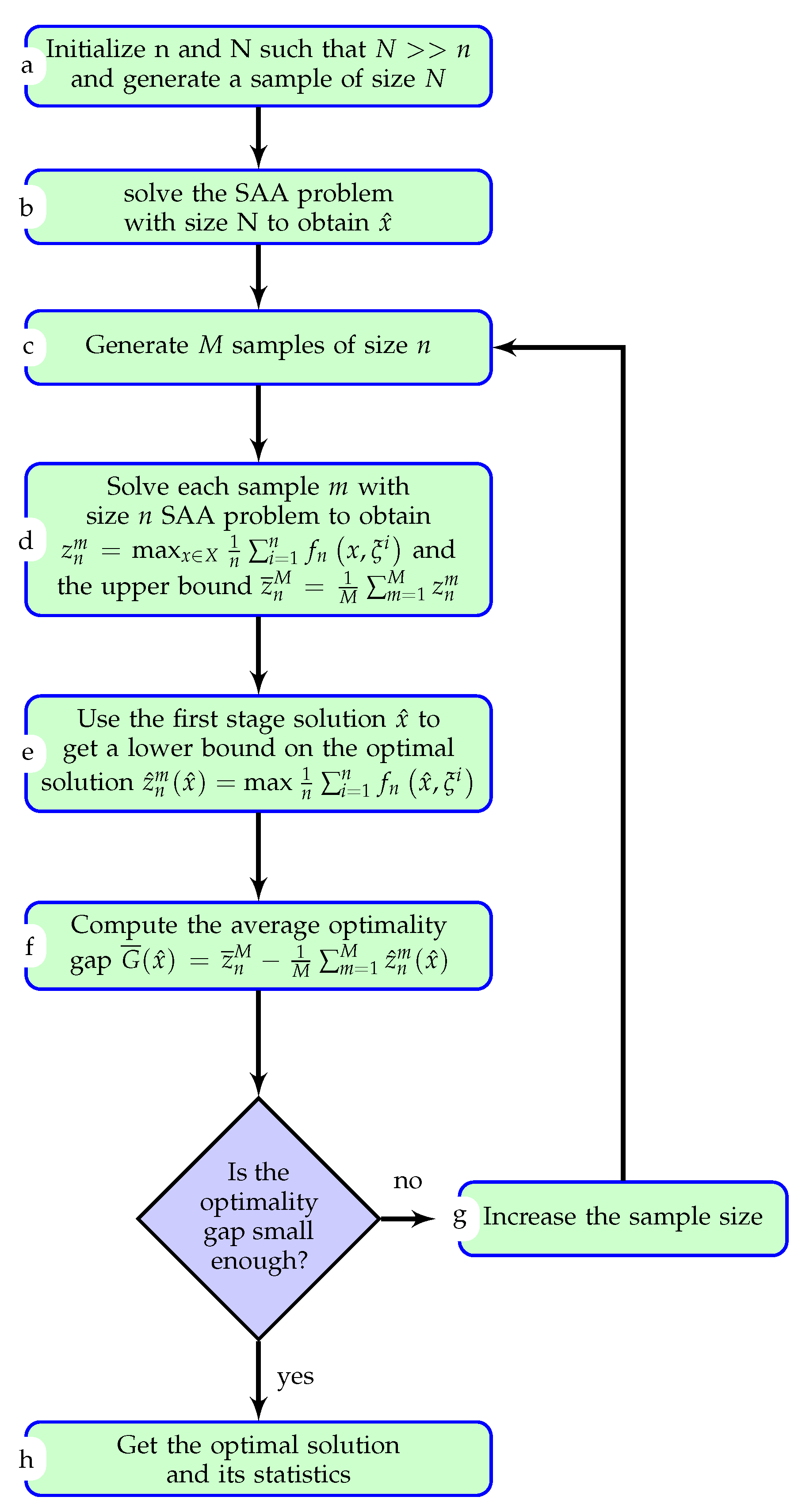
We now describe the steps for solving a stochastic optimization problem using SAA as outlined in
Figure 1.
Steps a and b: Generate a large sample of size (
N) and solve it using (
16) to obtain a first stage candidate solution
. The choice of
N depends on the model that can be solved in a reasonable time. The fact that this problem is only solved once, partially motivates on choosing the largest possible sample size.
Step c: Generate
M samples of size
n. The idea is to start with lower values of
n and increase the sample size progressively. Ref. [
24] describes a procedure for choosing the value of
M. In a nutshell,
M should be chosen in a way that allows to compute different statistics such as the mean, variance and confidence interval.
Step d: Solve SAA problem of each sample m to get and the upper bound . is an upper bound because it is the average of upper bounds obtained by using only a set of scenarios, and therefore the solution is more optimistic.
Step e: For each sample m, fix the first stage variables to obtained from steps a and b to get a lower bound on the optimal solution
Step f: Compute the average optimality gap as
. We can also compute for each sample
m the optimality gap as
where
is obtained by fixing the first stage variable in
to
from Step a. Notice that
. We can then compute the average optimality gap
and its variance
. Mak et al. [
16] proved that the optimality gap depends on the sample size
n. In fact, they proved that as
, the optimality gap converges to zero and the SAA objective function value converges to the true optimal objective value with probability one. In other words, the sample size is large enough if we have a small optimality gap.
Step g: If the optimality gap computed in step f is not sufficiently small, then increase the sample size n and go back to step c. The decision of whether the optimality gap is sufficiently small and its variance is sufficiently low is domain specific.
Step h: If the optimality gap is small enough, then we have obtained the optimal solution and we can compute the confidence interval on the optimality gap as: with a confidence of with being Type I error.
2.5. Importance of SAA
To assess the advantage of solving the stochastic optimization problem with SAA instead of the deterministic model that only considers the average scenario (the model that ignores climate change uncertainty), we compute the so-called value of stochastic solution (
) [
25]. Let
be the first stage solution we would get if we implemented the average growth solution, respectively. Similarly, let
be the optimal solution of the stochastic model obtained from SAA. We denote by
and
the NPVs of the scenario
when the first stage variables are fixed to
and
, respectively. Finally, let
whereas,
. We compute
as follows:
In term of relative value, we present
in basis points (bps) (1 basis point is equivalent to 0.01%. It is commonly used in economics and finance) as:
In case where some scenarios are not feasible after fixing the first stage to , we report the number of infeasible scenarios.
2.6. Experiment
We present in this section, the values of several parameters introduced in the methods in order to conduct a numerical experiment. The numerical experiment was run on a Windows desktop with an AMD 8 Core processor of 4 GHz and 8 GB of RAM. We have used CPLEX 12.8 to solve the stochastic model using python 3 as the modeling language. We solved each model to 0.5% mixed integer programming (MIP) optimality gap. For each model, we generated 30 independent replications (
). We used bootstrapping to compute the 95% confidence level for different metrics.
N was set to 625 scenarios and we varied the sample size
n from 16 to 625. We tested the modeling on Phyllis Leeper forest with 89 stands (
http://ifmlab.for.unb.ca/fmos/datasets/PhyllisLeeper/). Model parameters
and
were set to 0.85, whereas
and
were set to 1.15. The planning horizon was 50 years divided into 5 planning periods of 10 years each.
4. Discussion and Conclusions
Climate change is a serious issue in forest management planning. In a study conducted in Norway, the majority of forest managers showed the importance of addressing climate change in forest planning [
26]. Several researchers conducted similar studies in different ecosystems and reached analogous results [
27,
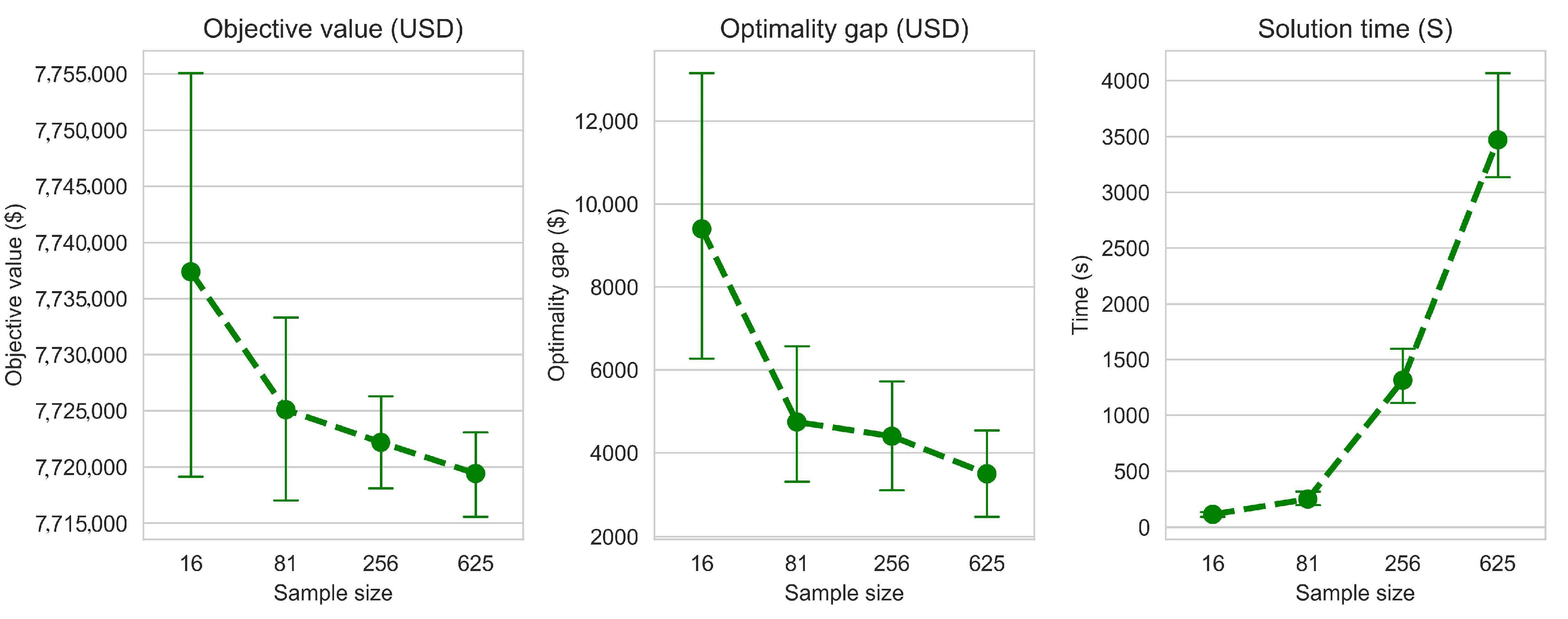
28]. To ensure the sustainability of forest resources, forest managers need to incorporate forest growth uncertainty in harvest scheduling models. In this work, we formulated a stochastic harvest scheduling model with forest growth uncertainty due to climate change and solved the model using sample average approximation (SAA). We tested the modeling and solution using climate change data transformed to forest growth change. We compared the robustness of the stochastic solution to the deterministic one by randomly generating a set of scenario and comparing the expected NPV if we implement the stochastic solution and the NPV if we use the deterministic solution. The numerical results showed that SAA allows to have stochastic solutions that are close enough to the true optimal solution when the sample size is large enough. However, large sample size leads to an exponential increase of solution time. This pattern of the computational complexity growing exponentially with the sample size was previously suggested by Kleywegt et al. [
24].
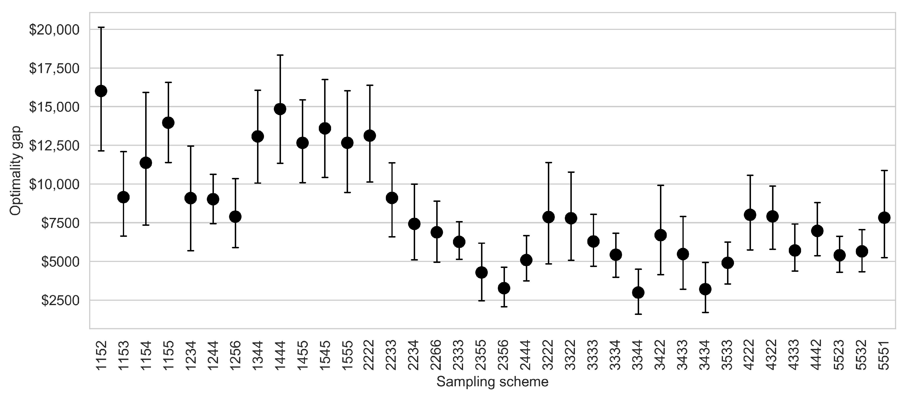
One of the main limitations of the proposed method is the computation required in step d of the algorithm presented in
Figure 1. As we discussed in the previous paragraph, the increase of the sample size leads to an exponential increase in solution time. It is therefore important to have a strategy that allows to reduce the sample size while producing solutions that allow the convergence of SAA solutions to the true optimal solutions. Our tests suggest that with the appropriate sampling scheme, it is possible to reach convergence with smaller sample sizes. For instance, the sampling schemes
2356 and
3344 yielding sample sizes of 180 and 144, respectively, have smaller optimality gaps and variances compared to a sample size of 625 which stemmed from a sampling scheme of
5555. In conclusion, when we adopt the adequate sampling strategy that allows to sufficiently explore the first stage and generate large samples for future stages, we can limit the number of scenarios necessary for the SAA solution to converge to the true optimal solution. This computational challenge is common to stochastic programs in forestry [
29].
The proposed model not only allows the managers to make intelligent decision now, but also allows the preservation of forest resources that take time to replenish once depleted. Indeed, the stochastic solution is robust to different growth scenario whereas, the deterministic one is infeasible to many of the tested growth scenarios. These results are in line with the ones obtained by Álvarez-Miranda et al. [
12], Garcia-Gonzalo et al. [
13]. The infeasibility of the deterministic solution stems mainly from the fact that the wood flow constraints are violated due to an intensive harvest in early periods.
In addition, the solution method proposed in this paper is easy to develop and implement by many forest managers. Unlike the methods used in [
11,
13] that require to know the probability distribution of the random parameter, SAA does not require such information. The method relies on the fact that if the sample size is large enough, then the sample statistics will approximate those of the actual population. The method is also suitable for many applications where the objective function cannot be computed in a closed form such as the so-called black-box optimization problems [
30] and the stochastic knapsack problem [
24]. In forestry, this method is well suited for harvest scheduling problems with wood price and demand uncertainties because we can extract samples from historical demand and price without the need to model the price like done in Alonso-Ayuso et al. [
10], Rios et al. [
31]. Compared to stochastic programming which requires the so-called non-anticipativity constraints [
13,
32], the SAA model is relatively smaller in terms of number of constraints (and possibly in terms of number of variables, depending on the formulation) since it does not require such constraints.
Regarding climate change data, we used the information of climate change forecast with statistical models developed in Latta et al. [
33]. Unlike the data from Garcia-Gonzalo et al. [
11], Álvarez-Miranda et al. [
12], Garcia-Gonzalo et al. [
13], which originated from a process-based modeling, statistical models of forest growth under climate change are much more common (e.g., Elli et al. [
34]). Hence, the method developed in this study can easily be extended to other forest systems. Moreover, it is straight forward to translate forecast of precipitation, air moisture and temperature into forest growth compared to processed-based models which require the expertise in plant biology.
Finally, this research can be extended by considering other sources of uncertainty such as the price of wood, or the demand of forest products. In this study we assumed that climate change does not lead to species transition. In some cases, one might need to consider the species shift because of climate change. It would be interesting to include this information in the decision-making process and provide to forest practitioners a range of options when implementing harvest scheduling plans and the choice of species for regeneration.


