1. Introduction
Information about timber volume and its distribution over forested area is an important prerequisite for forest management planning. For this purpose, forest inventories are usually conducted, where trees are measured in sample plots, and properties, such as timber volume per hectare, are calculated for each sample plot.
Since many years, remote sensing techniques such as airborne light detection and ranging (LiDAR) or aerial stereo photographs have been studied to obtain vegetation height [
1,
2,
3,
4,
5,
6], and to estimate timber volume or other forest properties in regression models [
1,
5,
6,
7,
8]. These models can be applied to the entire area for which a model is representative and for which the remote sensing data are available, resulting in area wide predictions of, for example, timber volume. This becomes particularly relevant when the timber volume of a smaller unit is of interest, for example of a forest stand or a forest district where not enough inventory plots are available to make reliable estimations [
9,
10].
The information about broadleaf and conifer trees improves timber volume modelling and reduces model errors and, thereby, prediction uncertainties (e.g., [
8,
11]). While there are several approaches to classify broadleaf and conifer trees, or even tree species using airborne LiDAR data (e.g., [
12,
13,
14,
15,
16]), optical data (e.g., [
17,
18,
19,
20,
21]), or a combination of both [
22,
23,
24,
25,
26,
27], these approaches are impractical for larger areas and reoccurring applications. LiDAR based approaches require either re-occurring surveys in leaf-on and leaf-off season to capture the difference between deciduous trees in summer and winter, or a very high point density to capture geometrical features of trees and their branches, which can be used for classifying broadleaf and conifer trees. However, LiDAR data collection is expensive and takes much time for large areas and at high point densities. Therefore, it is not feasible for large areas and regular, re-occurring surveying. Collection of optical data from aerial photography is less expensive compared to LiDAR data, but over larger areas the collection of this data takes much time as well. During large-area surveys, where it takes weeks or months to collect the data, development states of vegetation change affecting their spectral reflectance. Also, during data collection solar angles and solar radiation intensity changes, causing shadowing and affecting the illumination of the surface and, thereby, altering the spectral reflectance. Furthermore, modern cameras automatically adjust for situations with different illumination intensities to enhance contrasts, making it impossible to correct for the effects of varying illumination.
In contrast, satellite images cover large areas in very short time, do not have shadowing issues due to their perspective and coarser pixel size, and can be corrected for topographic and atmospheric influences. Satellite optical data have been successfully used in studies for classification of tree species [
17,
20,
21,
28] with overall accuracies exceeding 80%. Sentinel 2 images are available since 2015 and are collected by two satellites, resulting in a revisiting time of five days. The spectral bands of sentinel 2 images cover wavelengths relevant for vegetation analyses ranging from visible to red-edge, near infrared, and short-wave infrared with a ground resolution of 10 and 20 m (see
Table A1 in
Appendix A). The novelty of this data at this resolution is its free availability, offering a better alternative for spectral analyses and broadleaf-conifer classification compared to aerial photographs.
Forest management planning usually occurs regularly and on larger areas. To support forest management with remote sensing techniques on a regular basis, the availability of the remote sensing data must be guaranteed. The collection of aerial stereo photographs is less expensive compared to the collection of airborne LiDAR data, and can be used to compute 3D photogrammetric point clouds containing height information of the surfaces. Due to these limitations, many administrative bodies opt for using 3D photogrammetric point clouds to achieve regular and complete coverage of their geographic area.
The objectives of this study were to (1) model the percentage of broadleaf tree volume (BL%) using multi-temporal optical Sentinel 2 satellite images and forest inventory plots on a large and diverse geographic region in south-west Germany, and (2) model timber volume using 3D photogrammetric point clouds and forest inventory plots for the same area. This model can subsequently be applied for the entire area where the remote sensing data are available to produce spatially high-resolution growing stock data which is of great relevance for forest management planning, particularly for the assessment of standing volume of smaller units like stands by small area estimation procedures.
2. Materials and Methods
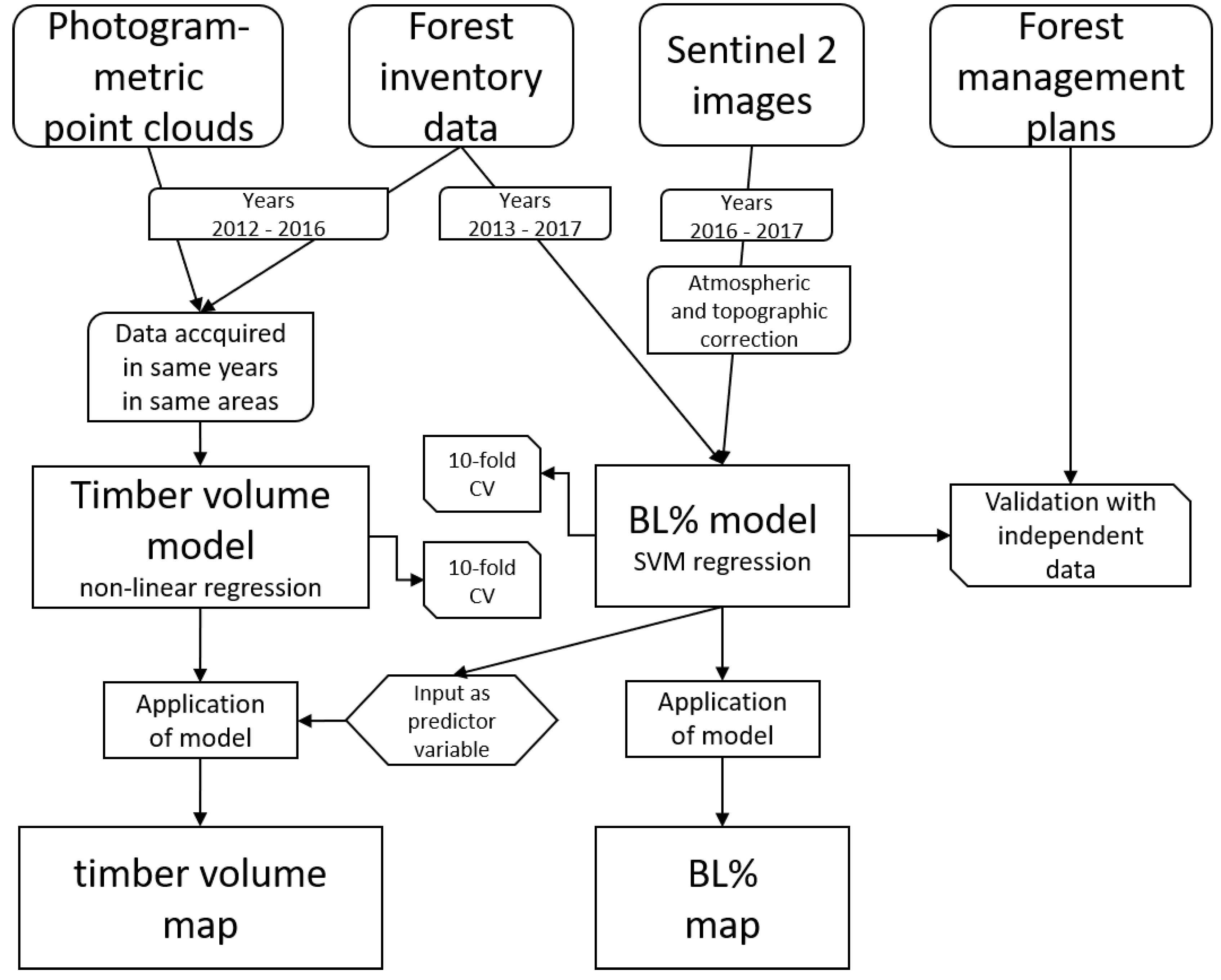
In the following we describe the data sets and the processing steps in subsections.
Figure 1 depicts the data set and the processing steps in a flow chart.
2.1. Study Site and Reference Data
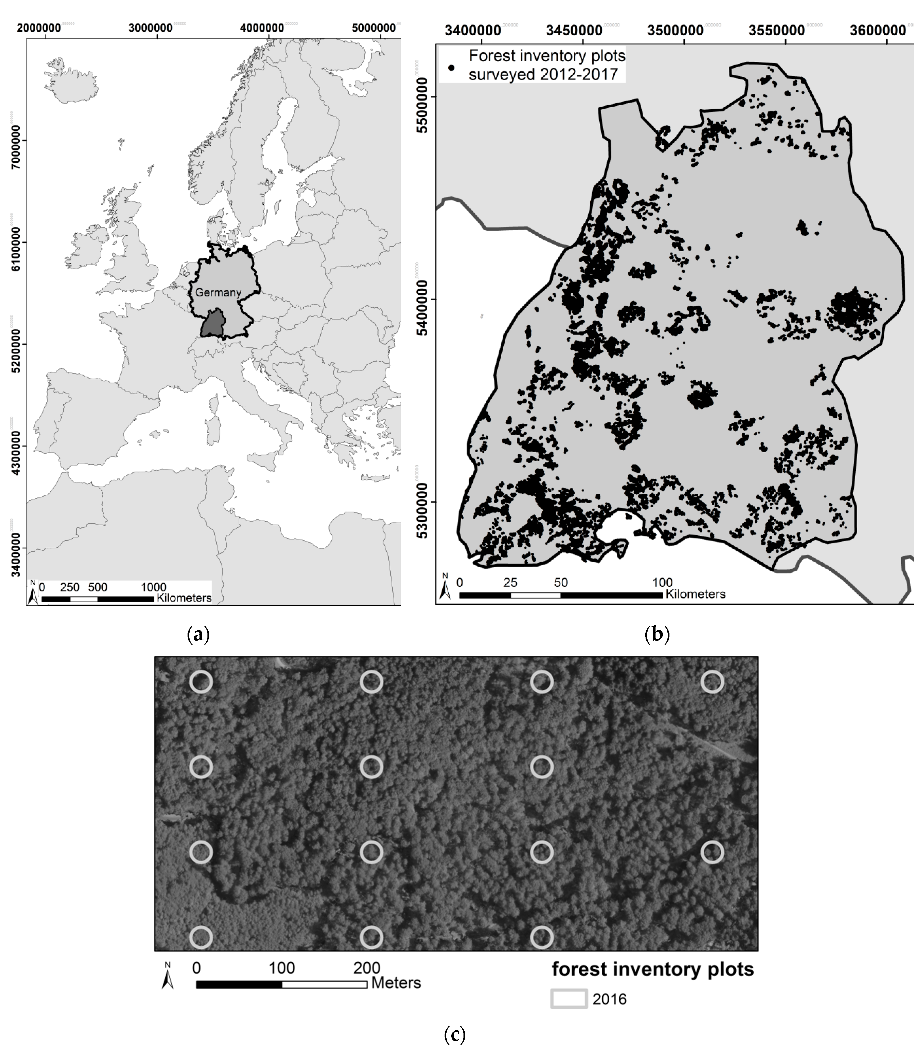
The federal state of Baden-Württemberg in the south-west of Germany with an area of 35,751 km
2 (
Figure 2a) was used as study site. This comprises diverse topographic conditions with altitudes ranging from 87 m above sea level in the Rhine valley to 1493 m above sea level in the Black Forest mountain range. Therefore, the forest varies greatly in terms of tree species composition and is dominated by Norway spruce (
Picea abies L., 34%), beech (
Fagus sylvatica L., 21.8%), fir (
Abies alba Mill., 8%), oak (
Quercus sp.
Thunb., 7.1%), pine (
Pinus sylvatica L., 5.6%), ash (
Fraxinus excelsior L., 4.9%), maple (
Acer pseudoplatanus L., 3.7%), and Douglas fir (
Pseudotsuga menziesii Mirb., 3.4%).
The forest area in this state comprises 1,371,886 ha. This area divides into state forest (23.6% or 323,765 ha of the total forest area), communal forest (40% or 548,754 ha), and private forest (35.9% or 492,507 ha). In this study, only data from state and communal forest was used, which together encompasses 872,519 ha forest. In this forest area 86,388 forest inventory plots of the forest enterprise inventories were located, which were surveyed between 2012–2107 (
Figure 2b). The forest enterprise inventories use a systematic sampling design with a regular grid, aligned with the Gauss-Krüger coordinate system, of 100 m × 200 m for larger forest estates (>200 ha), whereas for smaller ones a grid of 100 m × 100 m is used to ensure sufficient number of plots (
Figure 2c). The plots were geolocated by the field crews using a Global Navigation Satellite System (GNSS) device. During the terrestrial survey GNSS consumer-devices were used for locating sample plots, as their accuracy (5 m to 9 m) is considered sufficient for both installing new sample locations as well as for finding the center of existing sample plots in case of repeated measurement. Each circular plot has a radius of 12 m and is divided into three concentric circles with radius 3 m, 6 m, and 12 m. Diameter at breast height (1.3 m above ground) was measured by tape for all trees with diameter larger than 10 cm and smaller than 15 cm in the 3 m circle, trees with diameter larger than 15 cm and smaller than 30 cm were measured in the 6 m circle and only trees larger than 30 cm were measured in the 12 m circle. For each sample tree, azimuth and distance to the plot center, as well as species was recorded, amongst other variables. For height measurements, field crews used Vertex hypsometers (manufactured by HAGLÖF SWEDEN AB, Klockargatan 8, 882 30 Långsele, Sweden) with ultra-sonic measurement of the horizontal distance. Accuracy strongly depends on stand conditions (density, visibility of the tree tops) and is expected to vary between 1 m to 2 m for conifers (taller than 20 m). With deciduous tree species height measurements are less accurate due to crown morphology, namely with broadly spreading crowns, and may vary between 2 m and 4 m. As tree height measurement in the field is rather time-consuming these measurements were restricted to a subset of the trees: trees are assigned to specific species-groups and for each species group one or two well visible sample trees are selected for height measurement. Height imputation for trees without height measurement is based on the height-diameter relationship represented by species-specific uniform height-curves which are calibrated at sample level by means of the measured heights, similar as described in [
29].
From all inventory plots, only full plots (452 m
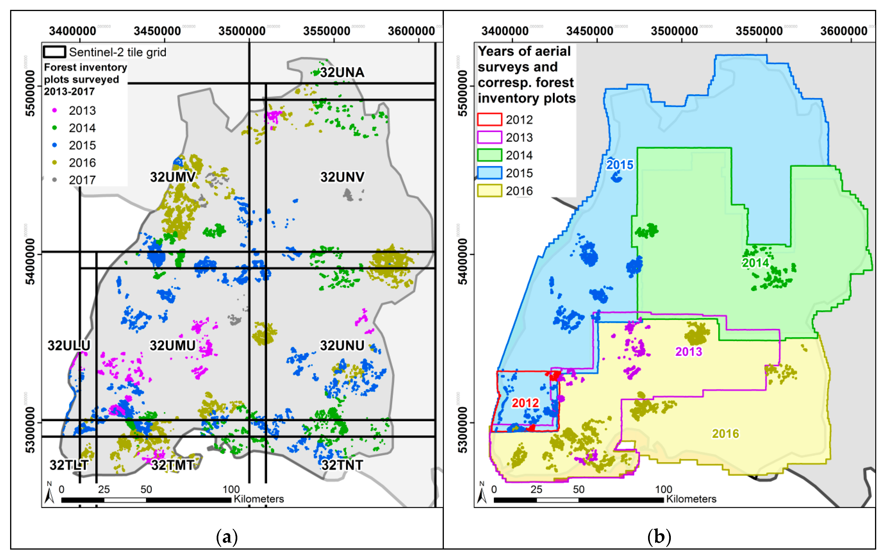
2) were used. Plots cut off by intersecting borders such as forest roads or forest borders, were discarded. Also, plots in which forest management activities were conducted since the last inventory were removed. Furthermore, to detect errors in the data related to geolocation of inventory plots or in the 3D point clouds, maximum and mean heights from the inventory data and from the 3D point clouds were compared using linear models. For this purpose, all points from the 3D point cloud falling into the inventory plots were extracted, and maximum and mean heights for each plot were calculated. Linear models were fitted with maximum and mean height from the inventory data as response, and maximum and mean height from 3D point cloud values as predictor variables. 95% prediction intervals were calculated from these models, and all plots outside the 95% prediction intervals were removed. From this set of inventory plots two subsets were selected; for modelling BL% using Sentinel 2 data, all plots from the years 2013–2017 were used resulting in 24,788 plots (
Figure 3a); for modelling timber volume using 3D photogrammetric point clouds from aerial stereo images, only those plots were selected, that were located in areas where aerial stereo photographs were collected in the same year as the forest inventory data, resulting in 11,554 plots (
Figure 3b).
Forest management plans are updated every ten years by forest experts appraising forest stands in the field. These forest stands were used as an independent data set to evaluate the performance of the BL% modelling. Forest stands, for which only broadleaf or only conifer trees were recorded, were selected, resulting in 13,778 stands with mean size of 1.42 ha.
2.2. Remote Sensing Data
2.2.1. Sentinel 2 Satellite Images
The two Sentinel 2 satellites are equipped with multispectral sensors, which detect a broad electromagnetic spectrum (443 nm to 2202 nm) in 13 bands (
Table A1 in
Appendix A). Three of these bands (1: coastal aerosol, 9: water vapour, and 10: short-wave infrared (SWIR) cirrus) are used for measuring atmospheric properties, and in this study were only used for atmospheric correction of the images. Sentinel 2 (S2) images acquired between January 2016 and April 2017 were downloaded through the Copernicus Open Access Hub (
https://scihub.copernicus.eu/) as top of atmosphere (TOA) reflectance images (named level 1C products). Only S2 scenes with less than 5% cloud cover were downloaded and visually inspected for their suitability. The spectral bands that were used for modelling BL% are available in 10 m and 20 m resolution (
Table A1 in
Appendix A). Nine S2 tiles were necessary to cover the study area (
Figure 3b). For each S2 tile, scenes from multiple dates were downloaded to depict the vegetation over various stages during the vegetation period. For one tile scenes from seven dates were used for development of the method, and for the remaining tiles scenes from four dates were initially downloaded. The program sen2cor (
http://step.esa.int/main/third-party-plugins-2/sen2cor/) was used to perform topographic and atmospheric corrections to obtain bottom of the atmosphere (BOA) reflectance images (named level 2A products). The standard settings of sen2cor were applied, and the 90 m Shuttle Radar Topography Mission (SRTM) digital terrain model (DTM) was used for topographic correction. Details for this process can be found in [
30]. All 20 m bands were resampled to 10 m resolution and saved as GeoTIFF files.
2.2.2. Aerial Image Based Canopy Height Model
The federal state of Baden-Württemberg in south-west Germany is surveyed in a three years cycle to obtain full coverage with aerial stereo photographs. In this study we used digital aerial stereo images acquired during these regular aerial surveys of the Baden-Württemberg land surveying authority (LGL). The aerial imagery is characterised by a forward overlap of 60%, side overlap of 30%, and a nominal ground resolution of 20 cm. The images were acquired by large size digital aerial matrix cameras (UltraCam Eagle, UltraCam SXp, UltraCam Eagle Prime, Ultracam Falcon (Vexcel Imaging GmbH, Graz, Austria) and DMC II (Leica Geosystems AG, Heerbrugg, Switzerland)) in 20 survey flights in June 2012, July 2013, May and June 2014, May–July 2015, and June–August 2016 (
Figure 3b). The images were recorded with four spectral bands (red (R), green (G), blue (B), and near infrared (NIR)), and a focal length between 79.8 mm and 100.5 mm. According to LGL, the orientation accuracy after aerotriangulation was between 0.03 m and 0.05 m in planimetric coordinates (
x and
y) and between 0.06 m and 0.14 m in height (
z) on control points. The data delivery from LGL included the imagery and an Inpho project file that comprised the exterior and interior orientation, ready to be used for subsequent photogrammetric processing. In addition, a high quality DTM with 1 m resolution was also provided by LGL. The DTM was derived from airborne laser scanning (ALS) data collected between 2001 and 2005, with an approximate point density of 0.8 points per square meter. The nominal height accuracy of this ALS-DTM reported by LGL is 0.5 m or better [
31].
A high resolution (0.4 m) 3D point cloud was generated from the stereo images in a dense image matching process using the software SURE of nFrames [
32]. Image matching was performed based on stereo image pairs and the results of multiple stereo pairs were subsequently fused [
33]. The implemented matching algorithm is a modification of the semi-global matching (SGM) algorithm proposed by [
34]. The software’s default parameter set for aerial images of the given overlap was used. Following adaptions were made according to the experience of the research team with image matching for forest areas: triangulation will accept a maximum angle of 99 and a minimum of 1 detections per cell. The interpolation for the extraction of a regular gridded point cloud was done with inverse distance weighted. A detailed description of the matching algorithm implemented in SURE can be found in [
35].
After point cloud extraction, all points identified as outliers were eliminated from each cloud. These outliers were identified in two steps. The first step considered the maximum tree height at the study site and the ALS-DTM available as reference. All points with elevations of 55 m and more above, and 1 m and more below the DTM, were regarded outliers and excluded from the point cloud. The upper threshold was based on the assumption that trees in this area are usually not taller than 55 m. The lower threshold allowed for some height inaccuracy in the point cloud. Within the second step noise reduction was performed by removing isolated points (n < 40) within a 3D box of 10 m in x and y and 4 m in height.
A standard process was applied to generate a canopy height model (CHM) from each filtered point cloud. First, a raster digital surface model (DSM) with spatial resolution of 1 m (equivalent to the resolution of the ALS-DTM) was derived from each point cloud using the software LAStools [
36]. Each DSM pixel value was determined by the elevation of the highest point within the planimetric pixel extent (1 m
2). In areas without matching points, the pixel values were calculated via Triangular Irregular Network (TIN) streaming [
37]. The CHMs with 1 m resolution were obtained by subtracting the ALS-DTM from the photogrammetric DSMs.
2.3. SVM Regression Modelling of Percentage of Broadleaf Trees (BL%) Using Sentinel 2 Data
In a first step, level 2A S2 data was prepared for the subsequent classification. S2 pixels representing areas covered by snow were identified by the pixel values of bands 4 (red, values larger than 1000) and 12 (SWIR, values smaller than 700) and filled in with the values of the next scene in the time series. Atmospherically and topographically corrected, cloud- and snow-free S2 band values were centered by subtracting the corresponding band means and scaled by dividing the centered bands by their standard deviation using the R function
scale from the
raster package [
38]. Subsequently, a principal component analysis (PCA) was conducted on all (resampled) 10 m bands. To reduce the amount of data to be processed, only every 20th pixel was used for calculating the PCA. PCA was performed in R [
38] using the function
prcomp from the
stats package.
In the second step, SVM Regression models were built for each S2 tile separately using the corresponding forest inventory plots. The variable BL% in the forest inventory data was used as response variable. As predictor variables all those PCA components were used that were needed to explain 90% of the variance. Therefore, the number of predictors for each model may vary. In this study we used a ε-SVM Regression with a RBF (radial basis function) kernel from the R-package “kernlab”. Two parameters were specified for this model: sigma as parameter for the RBF kernel, and the penalty factor C. These were optimized using the “train” function in the R-package “caret”. For ε the default value of 0.1 were used.
On one S2 tile (32UMV) all combinations of 1 to 7 scenes were used for modelling BL% to assess how many observations in the time series resulted in the highest accuracies. The combination resulting in the best model was chosen and transferred to the remaining S2 tiles. If in one S2 tile not all scenes could be used due to cloud coverage, the model was fitted without that scene.
2.4. Validation of SVM Regression Models
Models were evaluated based on RMSE from a tenfold cross validation using the forest inventory plots. Each model fitted for a S2 tile was validated separately with corresponding inventory plots. Since the reference data were circular plots, which overlapped with S2 pixels to varying degrees, weighted means of the pixel values intersecting the plots were calculated. Additionally, model predictions for the entire area were evaluated. For this purpose, model predictions were aggregated for each inventory plot and categorized into three classes (broadleaf trees: >80% broadleaf trees; mixed forest: <80% broadleaf trees and >20% conifers; conifers: <20% broadleaf trees). A confusion matrix was built, and accuracies were calculated.
Furthermore, the independent data set obtained from the forest management plans and consisting of forest stands containing only one tree species each was used to evaluate predictions for the entire area. All pixels with model predictions falling completely inside a polygon were aggregated for each forest stand polygon and categorized into the same three classes as above. This way the class of each forest stand polygon was compared to only one predicted value. A confusion matrix was built, and the predicted classes were then compared to the tree species documented in the forest management plans.
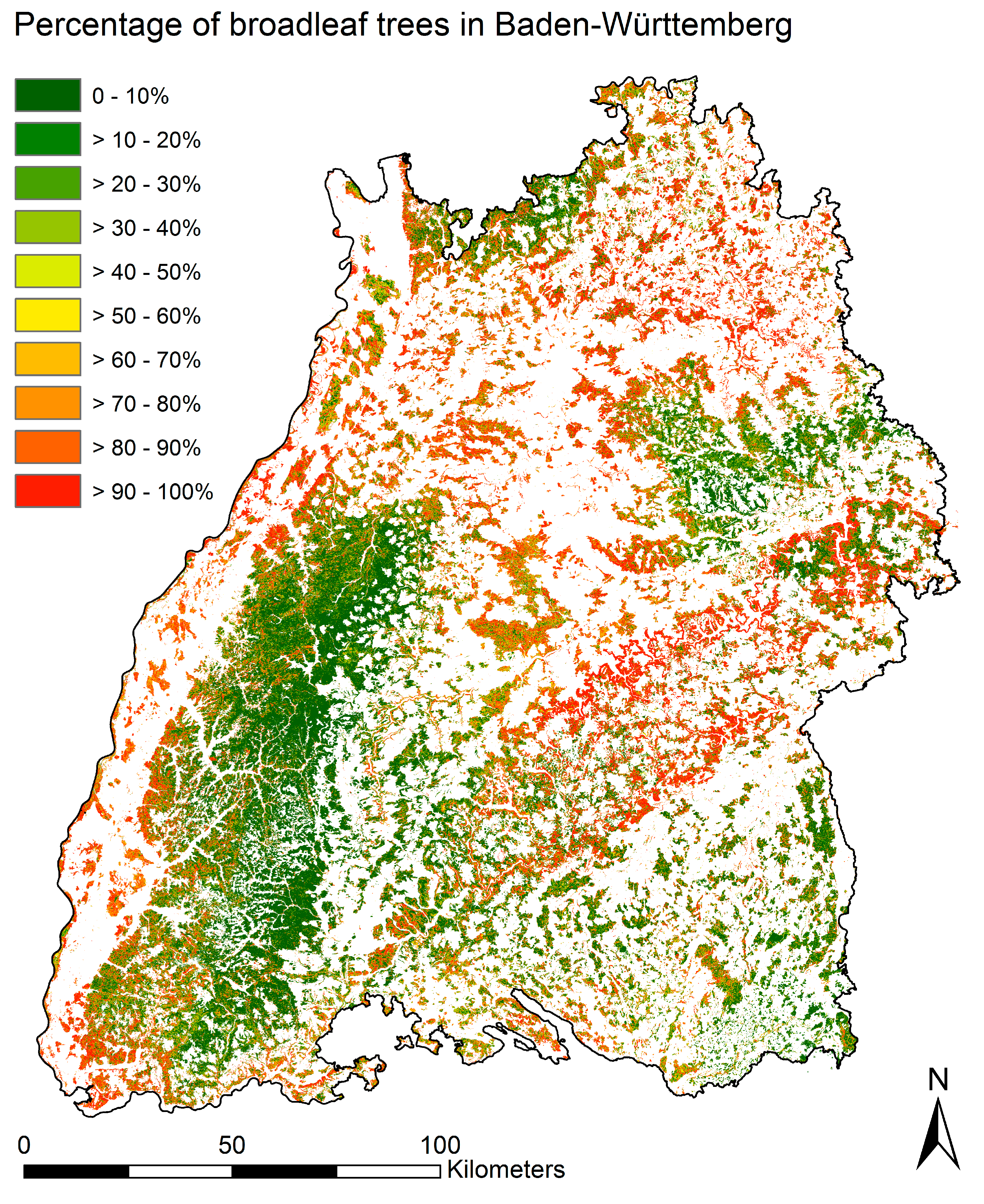
2.5. Mapping Percentage of Broadleaf Trees
Each model of the tenfold cross validation was used to make a prediction on the complete area. The results of these ten predictions were averaged for each pixel and thus give the final predictive value. In overlapping areas between the granules, the model with the better average RMSE value was used.
2.6. Regression Modelling of Timber Volume Using 3D Metrics from Photogrammetric Point Clouds
For each inventory plot, 25 plot-based descriptive metrics were calculated from the extracted CHM and DTM pixels. Those were 18 metrics related to canopy height—5th (p5), 10th (p10), 15th (p15), 20th (p20), 25th (p25), 50th (p50), 75th (p75), 80th (p80), 85th (p85), 90th (p90), 95th (p95), and 99th (p99) percentiles, arithmetic mean (CHMmean), minimum (CHMmin), maximum (CHMmax), standard deviation (CHMsd), variance (CHMvar), coefficient of variation (CHMcv), which are commonly used in other studies (e.g., [
39,
40]). One variable related to canopy cover and calculated as the percentage of CHM pixels ≥ 6 m (CHMcc). And six variables related to terrain—minimum (DTMmin), mean (DTMmean), and maximum (DTMmax) height above sea level, standard deviation (DTMsd), variance (DTMvar), and coefficient of variation (DTMcv) of the height above sea level. For model fitting, the information about BL% in each plot was obtained from the forest inventory survey.
In total, 26 metrics including BL% were used for timber volume modelling. Some of these metrics were highly correlated and a correlation analysis was conducted to avoid collinearity. Metrics that were correlated (Pearson) by more than 80% to each other were carefully examined and the metric that was most correlated with timber volume was kept.
Non-linear logistic regression models (
Table 1 Equation (1)), proposed by [
41] were fitted to the data set, and various combinations of the predictor variables selected in the correlation analysis were tested. As noted in [
40]: “This logistic regression model should not be confused with the binomial or multinomial logistic regression models that are often used with categorical data”. An advantage of this type of model is that the predictions are non-negative and are constrained by the upper horizontal asymptote β
K+2, which is estimated from the sample data. Also, linear models were tested, and nonlinearity in the data was handled by adding some of the predictor metrics additionally as squared terms to the models, and by transforming the response variable.
For each model, root mean square error percent (RMSE%) and bias% (
Table 1) of model predictions were estimated for each fold in a 10-fold cross-validation. For each model, RMSE% and bias% values from each fold were averaged. Additionally, standard deviation of bias% from each fold was calculated. Several models with varying combinations of predictive metrics selected in the correlation analysis were tested and the model with lowest RMSE% was chosen as best model.
2.7. Application of Timber Volume Model
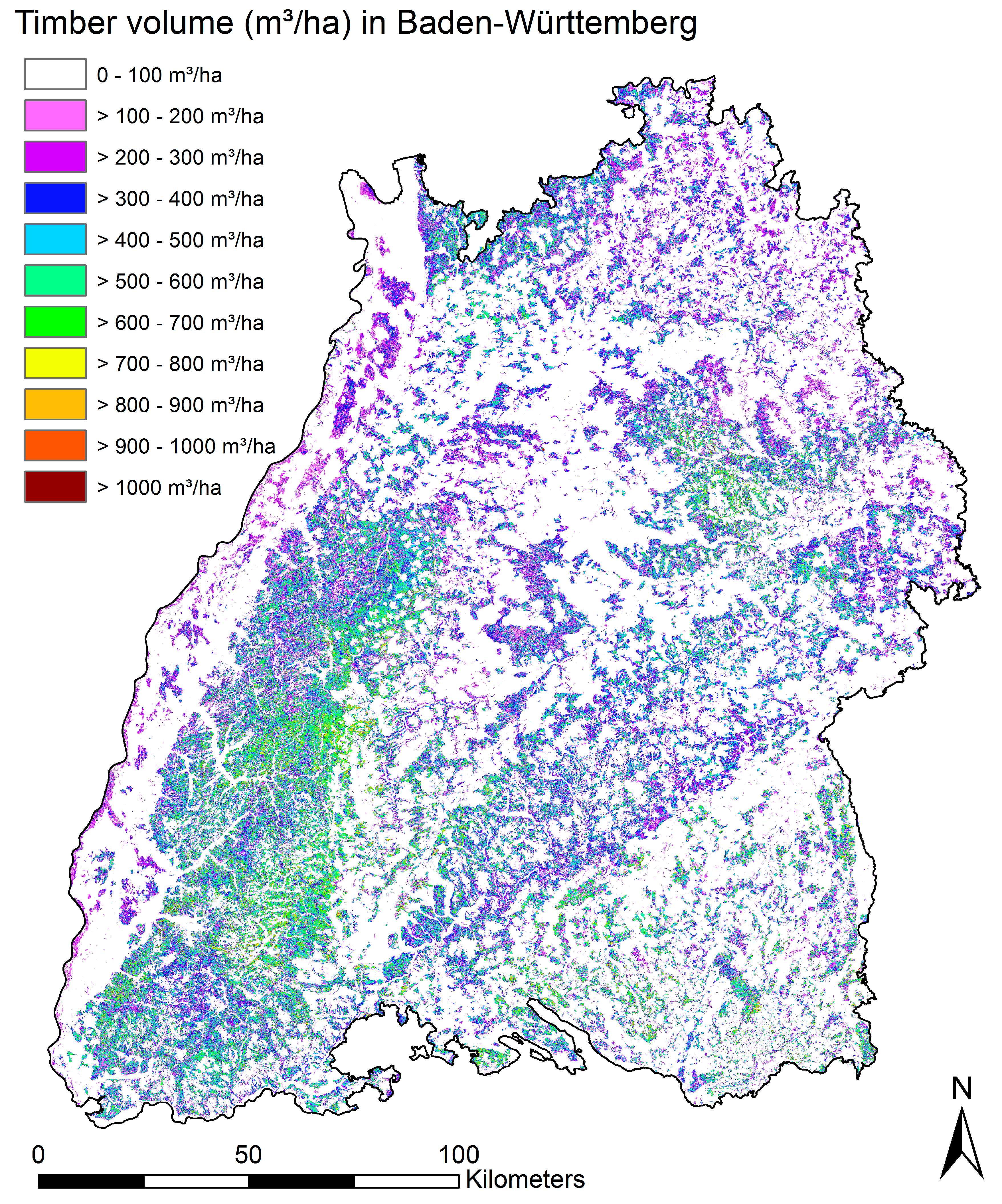
After model development we applied the model for the entire forest area for which the auxiliary remote sensing data was available, i.e., the entire federal state of Baden-Württemberg. For the entire area we calculated all predictor variables based on the CHM and DTM for 20 m by 20 m raster cells corresponding to the area of the forest inventory plots. Predicted BL% from the SVM model was resampled to the same resolution as the CHM, and then aggregated to 20 m by 20 m pixels as well. We then applied the regression model with the smallest RMSE% on each raster cell, resulting in timber volume predictions for the entire area.
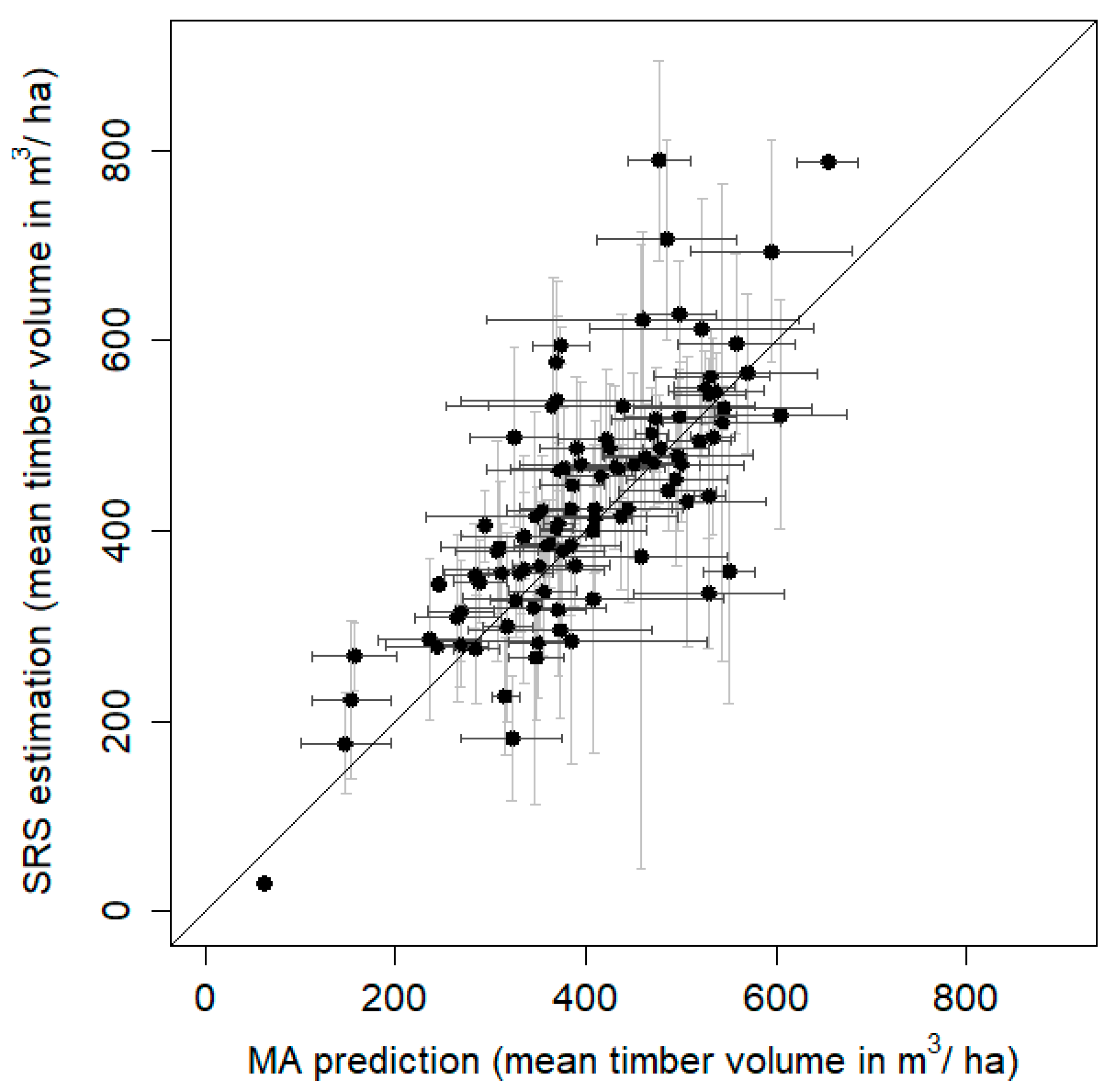
For 100 forest departments (a forest department consists of several stands and is a spatial administrative level in German forest management) in an area in the south-west of the state we aggregated predicted timber volume. Minimum, mean, and maximum area of these 100 forest departments were 10 ha, 32 ha, and 91 ha, respectively. Only pixels with predicted timber volume were used, that fell completely inside each forest district polygon to avoid edge effects. Mean timber volume and standard errors for each forest department were calculated using simple random sampling (SRS) with available forest inventory plots and model assisted (MA) small area estimation techniques [
42]. Equations are displayed in
Table 1, Equations (7–10). MA estimators use both models based on auxiliary data and SRS reference data. Estimates are expected to perform better compared to pure SRS estimates, since in MA estimation model predictions are used for all units where no sample plots are available, and available SRS reference data is used to correct for prediction errors to ensure unbiased estimates.
4. Discussion
In this study we present the development of forest tree type and timber volume maps for the federal state of Baden-Württemberg in south-west Germany. Recently, several studies have focused on the use of large-scale remote sensing data for mapping forest properties [
5,
43,
44,
45,
46]. Our study was motivated by the effort of the forest administration in Baden-Württemberg to support the field-work of the forest management experts by remote sensing-based information on forest resources for establishing forest management plans. In the following we will discuss the two parts of this study, modelling and prediction of percentage of broadleaf trees and timber volume.
In both models, BL% and timber volume prediction, uncertainties arise due to position inaccuracies of the reference inventory plots. The inventory plots have an unknown error in position accuracy due to inaccuracies of GNSS signals below forest canopy. This can result in a location of a plot several meters away from its assumed position. This leads to a shift between what is observed in the field and in the remote sensing data. More-over, the trees measured during forest inventory might not always be the same trees that can be seen from above, for example, when a large tree crown is overlapping other smaller trees. This will influence any model based on such auxiliary data estimating tree species.
The evaluation of the BL% models using cross validation resulted in good accuracies. The results of the evaluation on forest inventory plots were in line with the results on the independent data set based on forest management plans. The accuracies for the mixed class were relatively low. This was expected, since confusions between classes are most likely at class borders. These results fit into the general picture in this context and are in line with other studies. In a large-scale study in Norway, where three tree species spruce, pine, and broadleaf trees were classified using only a single date S2 scene, classification resulted in kappa of 0.59 for plots dominated by only one species, and in kappa of 0.5 when plots were included that were not dominated by a species group [
46]. In another study in central Sweden on a small test area, classification of five tree species spruce, pine, larch, birch, and oak using a time series of S2 scenes resulted in a kappa of 0.84 [
20].
The polygons from the forest management plans, which were used as an independent data set for the evaluation of the BL% model, were not selected based on random sampling. Instead, all polygons were used, for which only one tree species was recorded. Therefore, our results based on this data might be biased. However, we observed similar accuracies obtained with the forest inventory plots and cross validation. Therefore, we assume that the effect due to the non-random selection of the independent data is small.
The most important PCA components in the BL% model, and the importance of the original bands in the PCA were analyzed on the scene on which the method was developed. The PCA components 1, 2 and 4 were the most important predictors in the model. For PCA component 1 the original bands green, red edge and SWIR contributed with the highest loadings. For this component, these bands were used from all acquisition dates, but the winter scene contributed most. This indicates that this PCA component depicts the variation in these pixel values over time. PCA components 2 and 4 were dominated by bands NIR and red edge. For component 2, the spring scene was dominant, whereas for component 4 the winter scene was dominant. These results are in line with [
47], who also found that the red edge and SWIR bands are of high value for vegetation mapping.
Modelling of BL% was performed for each S2 tile separately for two reasons. The first reason was related to computational capacity and practicality. Tile wise processing is easier to standardize and requires less computational power than needed for a large mosaic. The second reason was related to small difference in pixel values in tiles of different paths that were collected at different dates, which occurred despite of atmospheric correction of the scenes. Another reason for modelling BL% on smaller spatial units is that vegetation states might differ between regions of low and high altitudes (e.g., earlier leaf flush in lower altitudes). Tile wise processing reduces this effect, even though differences in, for example, altitude and therefore phenology of vegetation might still occur in one S2 tile covering 100 by 100 km. A further development of this approach could include analyses based on regions corresponding to growing conditions or climatic zones. Nevertheless, the results achieved with the tile wise approach were satisfying.
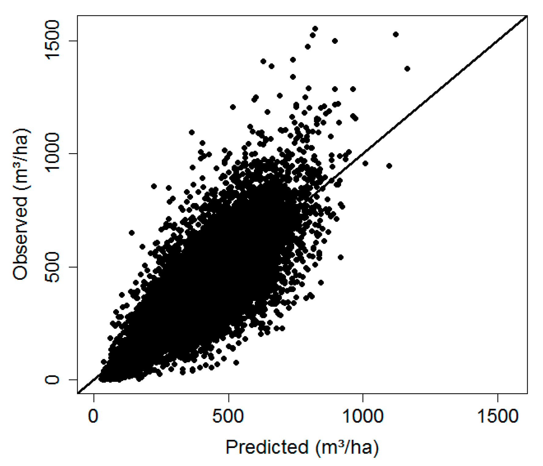
The timber volume model achieved an RMSE% of 31.7 from cross validation and a pseudo-R
2 of 0.64. This is similar to results of other studies, which used point clouds from stereo image matching and forest inventory data for the purpose of timber volume modelling. For example, RMSE% values of 31.92–37.89 were reported in a test area in Bavaria in Germany [
11], 28.8–32.9 in four different study areas in Sweden [
5], 31.43 in southeastern Norway [
6], 43.5 in central Norway [
48], and 36.87 in south-western Canada [
49].
The mean model estimates of timber volume per hectare in each of 100 forest departments showed good agreement with the estimates of the terrestrial reference sample (
Figure 5), and standard errors of the estimates were reduced by about 50%. For forest management planning, accuracy of timber volume estimation at stand level of about 10% is considered to be sufficient. Mean timber volume of all the 100 forest departments was about 400 m
3 per hectare. Our errors still amounted to a bit more than 10%, however, our model assisted errors were 50% smaller than what in this case was possible with terrestrial field data only.
For model fitting we used information on percentage of broadleaf trees from the inventory plots to obtain a model, which is as accurate as possible. However, when applying this model, error estimates of coefficients and, therefore, also of predictions might be too optimistic, since errors in the prediction of BL%, which are used as input variable in the model, are not accounted for. Using predicted BL% values instead of field observations for fitting of the timber volume model could be one approach, however, this would result in an error-in-variables model, which is beyond the scope of this study.
5. Conclusions
The combination of image based canopy height model with LiDAR based terrain model and Sentinel 2 data provided a suitable dataset for timber volume prediction covering large areas. Image based canopy height models were used for the description of tree height, canopy closure and canopy structure. Height above sea level, which was used as approximation for general growing conditions, was derived from the LiDAR based terrain model. Sentinel 2 time series served as input for the difference in volume-height relation between broadleaved and coniferous stands.
Aerial images from varying cameras with comparable flight parameters served as input for the extraction of canopy height models over large area. 3D point clouds derived from image matching were cleaned from outliers and noise before they were integrated into the surface model. A LiDAR based terrain model was used to normalize the surface model and to obtain the canopy height model.
Sentinel 2 time series with 3–4 images were suitable for the prediction of broadleaved percentage for large areas. This was valid for point validation (reference inventory data), as well as for area based validation (forest management plans). Tile based Sentinel 2 processing allowed for an adaption to the availability of cloud free data by tiles and varying time stamps. Within a Sentinel scene, missing pixels due to snow, clouds or cloud shadows, could be replaced with the pixels of the nearest Sentinel 2 scene within the time series. The processing results could be integrated into a single mosaic, covering the whole area.
Wall to wall timber volume predictions with a high spatial resolution of 20 m by 20 m were assigned to defined forest departments by MA method, according to the availability of inventory plots within respective departments, which resulted in 50% smaller standard errors compared to using filed inventory plots alone.

 ,
, 


