Predicting Growing Stock Volume of Eucalyptus Plantations Using 3-D Point Clouds Derived from UAV Imagery and ALS Data

Abstract

Estimating forest inventory variables is important in monitoring forest resources and mitigating climate change. In this respect, forest managers require flexible, non-destructive methods for estimating volume and biomass. High-resolution and low-cost remote sensing data are increasingly available to measure three-dimensional (3D) canopy structure and to model forest structural attributes. The main objective of this study was to evaluate and compare the individual tree volume estimates derived from high-density point clouds obtained from airborne laser scanning (ALS) and digital aerial photogrammetry (DAP) in Eucalyptus spp. plantations. Object-based image analysis (OBIA) techniques were applied for individual tree crown (ITC) delineation. The ITC algorithm applied correctly detected and delineated 199 trees from ALS-derived data, while 192 trees were correctly identified using DAP-based point clouds acquired from Unmanned Aerial Vehicles (UAV), representing accuracy levels of respectively 62% and 60%. Addressing volume modelling, non-linear regression fit based on individual tree height and individual crown area derived from the ITC provided the following results: Model Efficiency (Mef) = 0.43 and 0.46, Root Mean Square Error (RMSE) = 0.030 m³ and 0.026 m³, rRMSE = 20.31% and 19.97%, and an approximately unbiased results (0.025 m³ and 0.0004 m³) using DAP and ALS-based estimations, respectively. No significant difference was found between the observed value (field data) and volume estimation from ALS and DAP (p-value from t-test statistic = 0.99 and 0.98, respectively). The proposed approaches could also be used to estimate basal area or biomass stocks in Eucalyptus spp. plantations.

1. Introduction

Sustainable forest management demands accurate information that can be obtained efficiently and rapidly [1] in order to describe forest structure and quantify forest resources [2]. However, although accurate, traditional forest inventory is resource- and time-consuming, indicating the need for either alternative or complementary methods that may overcome the drawbacks of field data acquisition [3]. In addition, although field-measured data are commonly assumed to be ground truth values for remote sensing estimations, the associated errors tend to be large [3,4,5,6].

A number of alternatives to traditional field-based measurement of morphological parameters for characterizing three-dimensional (3D) structure of trees and canopies have emerged [4,7]. Airborne Laser Scanning (ALS), Digital Aerial Photogrammetry (DAP) and Terrestrial Laser Scanning (TLS) have become widely established as forest mapping and monitoring methods [8,9,10,11]. In the last two decades, DAP, ALS (e.g., [12,13,14]) or a combination of these methods (e.g., [15,16,17]) have been increasingly used to support forest inventories at different scales.

ALS has been the primary source of 3D data on forest vertical structure since the 1990s [18,19]. There has been an abundance of research demonstrating the utility of ALS for predicting forest biophysical variables to support forest inventories at individual tree- and stand-level [20,21]. Since the late 2000s DAP has provided a promising alternative, as the accuracy of stand-based estimates has been found to be similar to that achieved through ALS, at much lower cost [17,22,23].

Baltsavias [12] provided a comprehensive comparison of DAP and ALS data, highlighting the advantages and disadvantages of both technologies with regards to acquisition, accuracy, maturity and costs. Although ALS data have many advantages (e.g., direct measurement of height, higher penetration through the vegetation), DAP still represents an essential source of data for the forest inventory analyses. In fact, photogrammetric software has developed rapidly in the past 15–20 years. Since the first studies [24], advances in computer vision, image matching algorithms and computing power have promoted the use of aerial images for generating high-resolution 3D data by image matching [25]. Many photogrammetric software packages (proprietary and open-source) have been developed, offering unparalleled opportunities to produce 3D data from 2D image collections with high overlap.

Recent advances in sensors and in image processing –particularly Structure from Motion (SfM) technology– have also enabled the extraction of dense point clouds obtained by DAP [16,24,26,27,28,29]. In this sense, DAP derived from SfM is an emerging source of 3D data, reaching quality standards close to those provided by ALS [25,30]. works by [26,31,32,33] pointed out the potential of DAP for forest applications. During the past five years in particular, there has been an increasing interest in the use of DAP to generate 3D data analogous to ALS data, in order to support forest inventories [17,22,25,34,35,36,37,38,39]. This interest can be attributed to the need to optimize costs while improving the temporal resolution.

Unmanned Aerial Vehicles (UAVs), also known as drones or Unmanned Aerial Systems (UAS), have emerged as a cost-effective alternative to conventional methods based on manned fixed-wing aircraft or helicopters for DAP imagery and ALS data collection [40,41,42,43]. Since the first studies in which UAV-derived data was used for forest inventory purposes [44,45], UAV-based forestry applications of both ALS and DAP have increased substantially [40,46,47,48,49,50,51,52]. Indeed, ALS and Red-Green-Blue (RGB) sensors mounted on UAV platforms are becoming cost-effective tools for monitoring forest structure because of their high spatial and temporal resolution, achieved by the low flight height, operational flexibility and relatively low cost of the flight surveys, which meet most of forest managers requirements [53]. In particular, light UAVs equipped with inexpensive consumer grade cameras have recently appeared as a feasible option for monitoring 3D forest structure [54]. In addition, multi-temporal UAV-acquired data can also be used for rapid, accurate and cost-effective tree growth assessment, providing up-to-date information to support decision-making in forest management [48,54,55,56,57,58].

Two main strategies have been adopted for DAP and ALS-based analysis in forestry inventories: (i) the Area-Based Approach (ABA), a distribution-based technique which typically provides data at stand level, and (ii) the individual tree crown (ITC) delineation, in which individual tree crowns, heights and positions are the basic units of assessment. ABA has been used with ALS and DAP to estimate forest attributes over a wide range of forest types including Temperate (e.g., [59]), Boreal (e.g., [13,14,17,34,60]), Atlantic (e.g., [61,62]), Tropical (e.g., [37]), Alpine (e.g., [63,64]), Mediterranean forests (e.g., [65,66,67,68,69]) and plantations [70]. At the stand level, results from recent research on small- to medium-sized boreal and tropical forests have demonstrated the potential use of UAV-based DAP data for estimating forest biomass [53,71]. On the other hand, ITC has also been applied to DAP point clouds [72] and to ALS clouds [73,74]. ITC presents several advantages over ABA for estimation of above-ground biomass because it can be used to derive biomass when an allometric model is available at individual tree level [75]. At the same time, it is particularly well suited for precision forestry, which usually requires information about individual trees.

Finally, ALS and SfM approaches to tree height estimation tend to underestimate tree height [73,74,76,77]. Recent studies [77] have presented a model that explains the observed bias using probability theory, developing methods for correcting several ALS metrics used for ABA prediction of stand structure. However, few studies have evaluated the influence of this bias at individual-tree level. In this respect, further research is needed in order to analyze the influence of this bias in the individual-tree biomass and volume models for both technologies.

The objectives of this study were as follows: (i) to investigate the combined use of ALS- and SfM-derived individual-tree measurements (height and crown area) with non-linear regression models to estimate individual tree diameter and volume; and (ii) to compare the estimation of ALS- and SfM-derived individual-tree volume models to estimate growing stock volume in relation to field data.

2. Materials and Methods

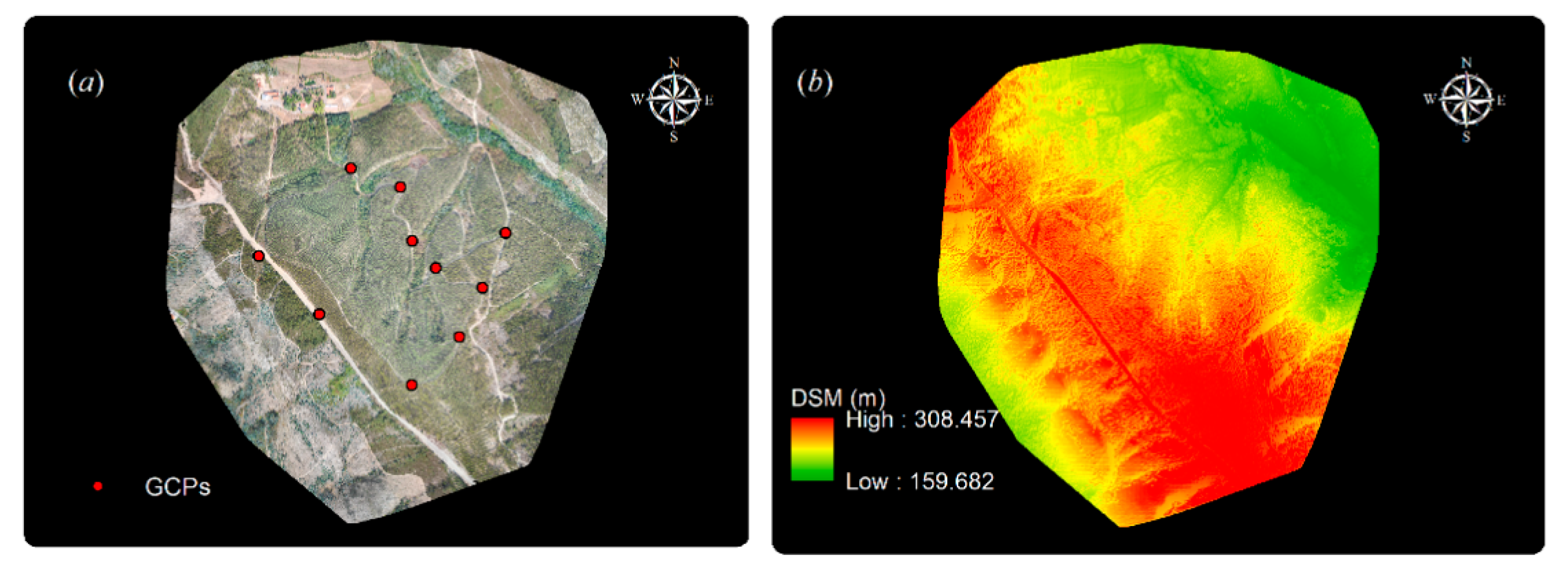
2.1. Study Area

The study area is located in the municipality of Valongo (41.213° N, −8.496° W) in the district of Porto, Portugal (Figure 1). The site consists of a seven year old plantation of Eucalyptus spp. clonal material (G74), covering an area of 26 ha. Tree spacing was 3.70 × 2.5 m, yielding a density of one tree per 9.25 m⁻². The elevation ranges from 163 to 294 m above the WGS84 reference ellipsoid. The terrain is topographically complex, with steep slopes (mean slope = 24.2%), and of elevation up to 131 m. The mean annual rainfall is 1568 mm, and 42.1% of the precipitation occurs between November and January. The mean annual temperature is 14.2 °C, ranging from 8.6 °C in the coldest months (December to February) to 20.1 °C in the warmest months (July to September). The study site is characterized by evenly planted trees of superior genetic material with a low mortality rate.

2.2. Field Measurements and Field Volume Estimation

The field data were collected in December 2016 (to correspond to the date of acquisition of ALS data) from 6 square plots, each of approximately 400 m² (

Table 1. Statistical description of the field data within six field plots for a total of 323 reference trees

Plot	d		h		$\widehat{\mathit{v}}$
	Mean		Mean		Mean
	Dec 2016	Sep 2017	Dec 2016	Sep 2017	Dec 2016	Sep 2017
P1	13.2	13.4	19.4	20.9	0.13	0.14
P2	12.9	13.3	18.8	19.9	0.12	0.15
P3	13.4	13.8	18.6	20.0	0.13	0.15
P4	13.8	14.1	18.8	19.8	0.13	0.15
P5	13.7	14.0	18.3	19.7	0.13	0.15
P6	13.8	14.2	17.6	19.1	0.13	0.14
Min.	5.3	5.4	9.9	10.3	0.01	0.01
Mean	13.5	13.8	18.6	19.9	0.13	0.14
Max.	17.3	17.8	22.8	23.5	0.24	0.26
SD	1.7	1.7	1.5	1.6	0.03	0.04

Average (Mean), minimum (Min), maximum (Max) and standard deviation (SD), values of the individual tree diameter (d, cm), height (h, m) and field data volume estimation ($\widehat{v}$, m³).

). A total of 323 reference trees were measured and located in 6 square plots (400 m²). The height of each tree (h, m) within the plots was measured with a Haglof Vertex IV hypsometer equipped with a T3 transponder. The diameter at breast height (1.30 m above the ground – d, cm) was measured with a steel diameter measuring tape. Field plots were remeasured using the same methods in September 2017 (matching with UAV-based DAP acquisition).

In order to obtain accurate positions of the trees, topographic surveys were conducted to determine the position of the center of each tree within the plots. A Trimble^® TSC3 GPS controller with Trimble^® R8s Integrate GNSS System Antenna (Trimble, Sunnyvale, CA, USA) (dual-frequency real-time kinematic receiver –RTK) was used to determine the coordinates of a densified geodetic network for the study area by applying real time kinematic (RTK). Based on the network established with GPS, a topographic survey of the plots was conducted using a Trimble^® M3 Robotic Total Station (Trimble, Sunnyvale, CA, USA). Observations on the position of each tree within the plot were made during the survey.

Field-derived volumes were estimated using the Equation (1), provided by [78].

$$\widehat{v} =0.2105 {\left(\frac{d}{100}\right)}^{1.8191} h^{1.0703}$$

(1)

where $\widehat{v}$ is the estimated volume (m³), d is the diameter (cm) at the breast height (1.30 m) and h is the tree height (m).

2.3. ALS Acquisition

The airborne surveys were conducted on 17 December 2016, covering an area of 100 ha. The data were captured with Leica ALS80-HP laser scanner operating at pulse rate of 704 kHz, field of view of 6.5° and scan rate of 73.5 Hz, which was mounted on a Cessna airplane that flew the area at an approximately flight altitude of 2750 m.a.s.l and an average speed of 250 km.h⁻¹. The overlap between sweeps was 30%, achieving an average laser pulse density of 43.33 pulses m⁻².

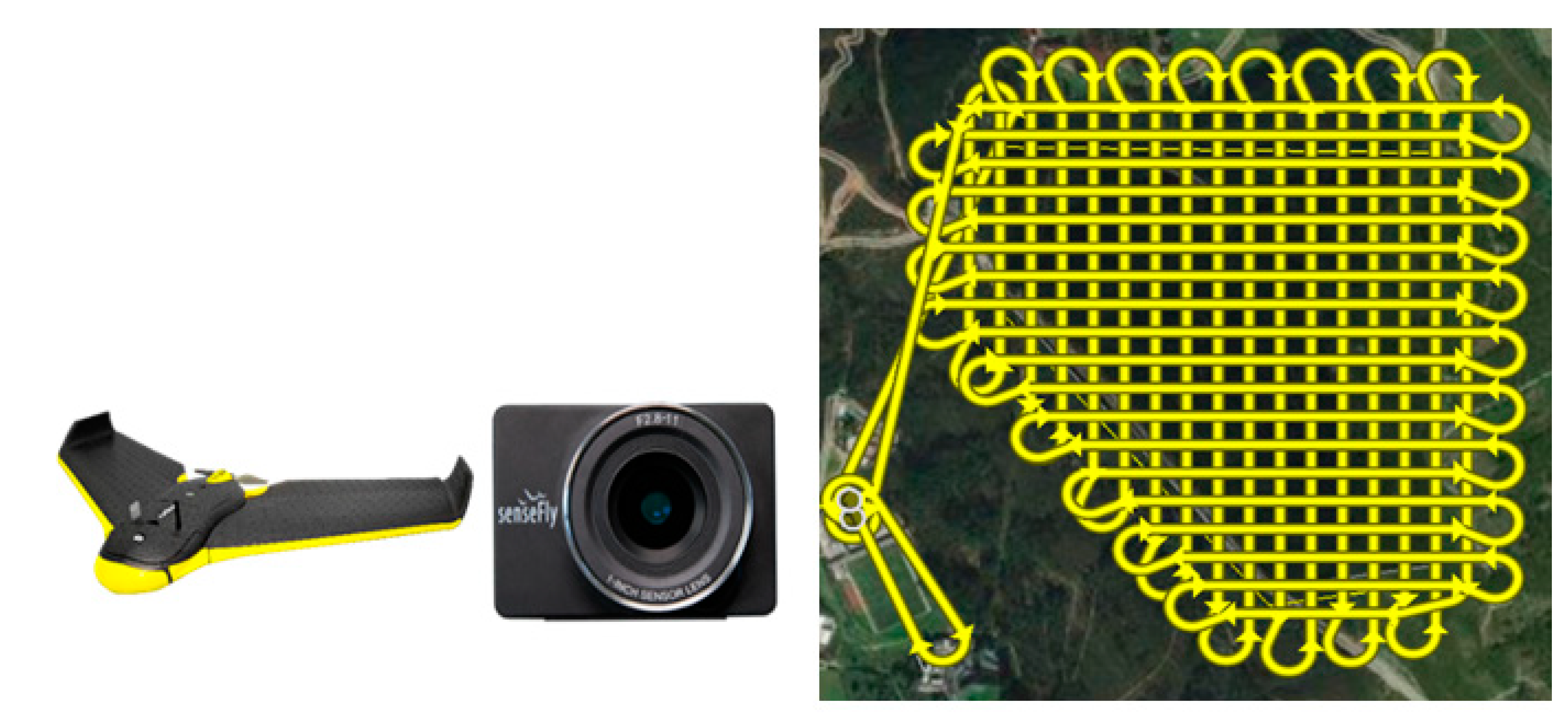
2.4. UAV Data Acquisition and Use

The airborne surveys were conducted on 6 September 2017. An RGB S.O.D.A. 10.2 (20 MP) camera (senseFly Co, Cheseaux-Lausanne, Switzerland) was mounted, with nadir view, on a fixed-wing UAV (SenseFly eBee) (Figure 2). The camera, which was equipped with a 12.75 × 8.5 mm sensor and 5472 × 3648 pixels detector, was used in manual mode. Exposure settings (ISO 150 and shutter speed of 1/1000 s) were set before each take-off according to the light conditions. This provided ~6 cm pixel⁻¹ resolution for a variable altitude above ground level, which is especially useful in areas of diverse elevation range such as mountainous regions. Atmospheric conditions during the airborne surveys were characterized by calm winds, clear lighting at the flight time (between 11.30 am and 12.15 pm) to minimize the effect of shadowing. Flight parameters were determined using eMotion V. 3.2.4 flight planning and monitoring software. The flight plan covered the entire study area with longitudinal and lateral overlaps of 85% in both cases. The flight line spacing was 25 m (Figure 2). In total, 744 images were used to generate orthomosaics and Digital Surface Models (DSMs) by the SfM image reconstruction process. Two-block flights were required to capture the entire forest study area (the orthomosaic covered an area 103.70 ha with average Ground Sample Distance (GSD) of 5.95 cm).

2.5. 3D Model Generation and Preprocessing Point Clouds

The absolute orientation of the aerial photos was determined using aerotriangulation techniques implemented in pix4D 3.3.29 (pix4D^®, Ecublens, Switzerland). A set of 10 ground control points (GCPs) measured in the field with topographic methods was used to georeference the SfM mosaics to a projected coordinate system for both datasets. The ground control photogrammetric points (GCPs) were captured with a Trimble TSC3 controller and a Trimble R8s GNSS antenna (RTK precision 8 mm + 1 ppm Horizontal/15 mm + 0.5 ppm Vertical) mounted on a pole. The GCPs markers comprised a set of 1 × 1 m cross-shaped white painted timber planks with some black and white 50 × 50 cm painted checkerboards. For reliable accuracy of GPS measurement, all GCPs were located in open areas with no canopy cover. At each point, GPS signals were logged in RTK–global navigation satellite system (GNSS) mode. The recordings were processed with real-time correction data retrieved from the fixed base station in Gaia (Porto) (latitude: 41°06′21.67048″ N, longitude: 8°35′20.73434″ W, and ellipsoidal elevation: 287.63 m above the WGS84 reference ellipsoid).

Photogrammetric point clouds were computed using SfM techniques, implemented in Pix4D 3.3.29. The matching parameters for point cloud densification were set as follows: multiscale, image scale = 1/2 (half image size) and point density = ‘optimal’. The minimum number of matched images was also set to 3. DEM_SfM was generated from the ground points by using a natural neighbor interpolation technique implemented in Pix4D (additional details of the algorithms are proprietary and were not disclosed by Pix4D).

The ALS and SfM point clouds preprocessed using FUSION/LDV 3.60 software [79] and LasTools [80]. For more details of point cloud processing see details in [74]. Finally, two CHMs (CHM_SfM and CHM_ALS) were obtained by subtracting the DEMs (DEM_ALS and DEM_SfM) from the DSMs (DSM_ALS and DSM_SfM) in the FUSION LiDAR Toolkit [79].

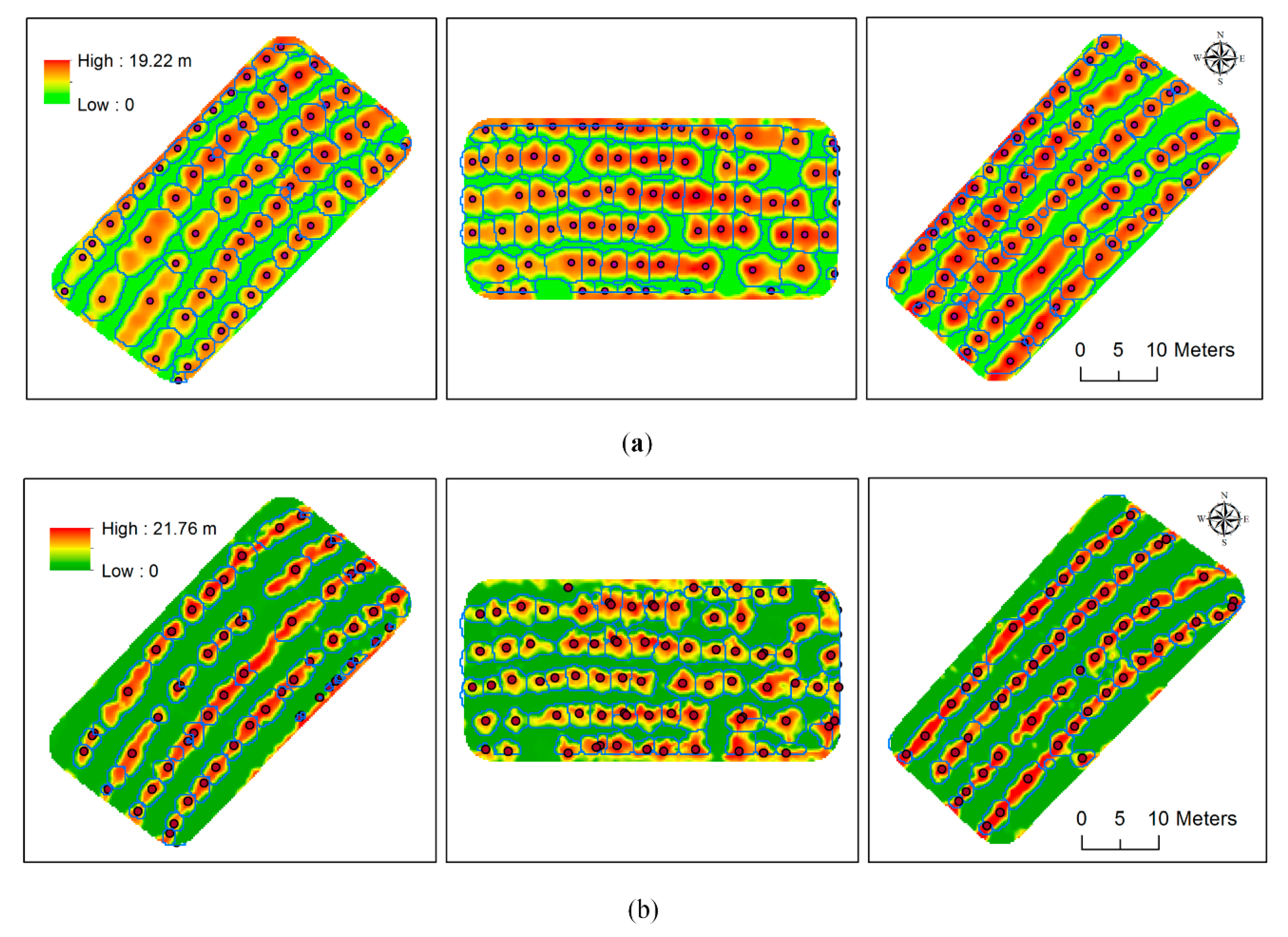
2.6. ITC Process to Derive ALS- and SfM-Variables

Individual tree position (X and Y coordinates), height (h_SfM, h_ALS) and crown area (ca_SfM, ca_ALS) were retrieved from the respective CHM_SfM and CHM_ALS (Figure 2). Resampling of the CHMs to 20 cm resolution and subsequent smoothing with mean filter (5 × 5 window) in the case of ALS and median filters (3 × 3 window) for SfM were conducted using the FUSION LiDAR Toolkit [79]. Crown delineation followed the procedure detailed in [81]. The process is divided into three main phases: segmentation, classification and iterative watershed segmentation The Chessboard Segmentation algorithm was used to split the image into square image objects. In the second phase, a Classification algorithm was used to classify image objects from the smoothed CHM. Objects with an elevation value of less than 5 m were classified as gaps. The threshold was established empirically from field observations and by trial-and-error tests. The remaining objects were assigned to the ‘temporary canopy’ class. These objects were used to locate tree tops and delineate tree crowns in the following iterative watershed segmentation processes. In the iteration, the Find Local Extrema algorithm was used to classify the image objects of the ‘temporary canopy’ class, which fulfills a local extreme condition according to image object features within a search domain in their neighborhoods. However, because of the forest stand and tree species characteristics, the initial maximum search domain used in the iterative process (see Figure 3 in [81]) to detect top trees was changed from 5 to 3, and 4 interactions were applied. A search with a variable square window enables detection of apices of trees with a large variety of crown sizes. Objects less than 3 m away from any detected tree top were retained in the ‘temporary canopy’ class (candidates for watershed) and any other objects were disregarded. This distance was the maximum observed crown width in the plots, which was considered the limit for crown growing in the next step. Then, the crown delineation results (Figure 3) and tree top positions were exported in ESRI^TM shapefiles as vector polygons and points respectively, for subsequent analysis.

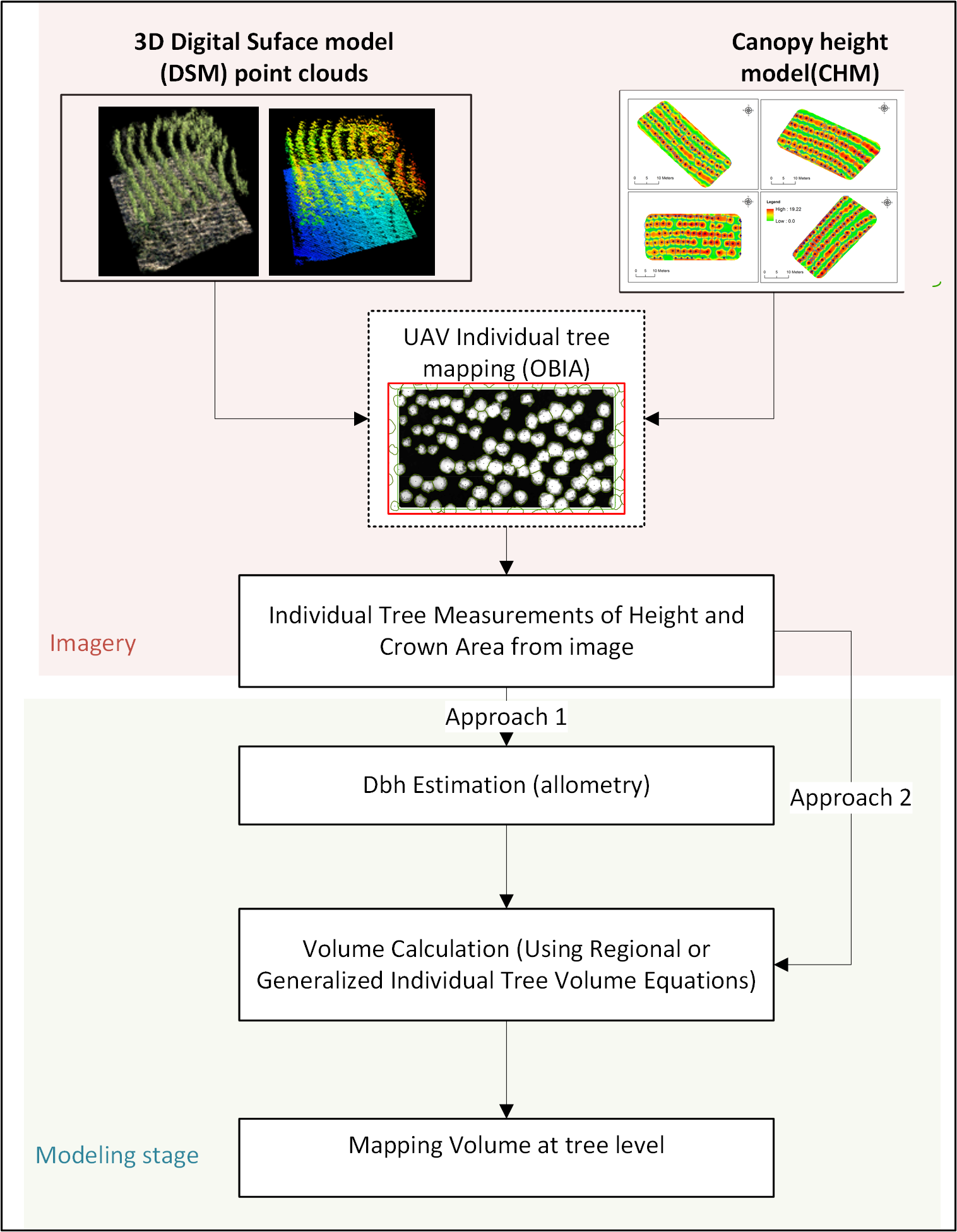
2.7. Individual Tree Volume Estimation

Volume equation (Equation (1)) requires the measurement of tree diameter or circumference, which is not available from UAV imagery. We therefore tested two approaches for estimating ALS- and SfM-derived individual-tree volumes (v_SfM and v_ALS) (Figure 4). In the first approach, the multiplicative (power function) model in Equation (2) was fitted using d (from field data) as the dependent variable and the pairs of explanatory variables h_SfM, ca_SfM for SfM, or h_ALS, ca_ALS for ALS. The predicted diameter obtained by each method (d_SfM and d_ALS) and their respective height estimates (h_SfM and h_ALS) were then included as independent variables in Equation (1) to predict the individual volumes for the subset of 192 trees for ALS and 199 for SfM (v_SfM and v_ALS, respectively). In the second approach, the multiplicative (power function) model in Equation (3) was also fitted to predict v_SfM and v_ALS for the 192 and 199 trees respectively, but v was considered a dependent variable (estimated using the field-measured d and h in Equation (1)), and the pairs h_SfM, ca_SfM (from SfM) or h_ALS, ca_ALS (from ALS) were considered explanatory variables, without the need to estimate the diameters.

$$\widehat{d}=h^{{\beta }_0}c{a}^{{\beta }_1}+\epsilon$$

(2)

$$\widehat{v}= h^{{\beta }_0}c{a}^{{\beta }_1}+\epsilon$$

(3)

where $\widehat{v}$ is the estimated volume (m³), $\widehat{d}$ is the estimated tree diameter (cm), h is the tree height (m), ca is the canopy area (m), generated from ALS or SfM, β₀, β₁, are the exponential parameters to be estimated by non-linear regression analysis; and ε is the additive random error. The models were fitted using the Non-linear Least Squares nls function implemented in the BASE package of R software (R Core Team, 2018).

Finally, the Model Efficiency (Mef, Equation (4)), the overall root mean square error (RMSE, Equation (5)), the relative root mean square error (rRMSE, Equation (6)) and the Bias (Equation (7)) were computed in order to determine the accuracy of ALS and SfM models for estimating diameter and volume with the second approach. Mef compares predictions directly with observed data using a statistic analogous to R² [82]. This statistic provides a simple index of performance on a relative scale, where 1 indicates a ‘perfect’ fit, 0 reveals that the model is no better than a simple average, and negative values indicate a poor model.

$$Mef=1-\left(\frac{\left(n-1\right){{\displaystyle \sum }}_{i=1}^n{\left(y_i-{\widehat{y}}_i\right)}^2}{\left(n-p\right){{\displaystyle \sum }}_{i=1}^n{\left(y_i-{\overline{y}}_{}\right)}^2}\right)$$

(4)

$$RMSE=\sqrt{\frac{{{\displaystyle \sum }}_{i=1}^n{\left(y_i-{\widehat{y}}_i\right)}^2}{n}}$$

(5)

$$rRMSE=\frac{RMSE}{\overline{y}}*100$$

(6)

$$Bias=\frac{{{\displaystyle \sum }}_{i=1}^n({\widehat{y}}_i- y_i)}{n}$$

(7)

where n is the number of trees; y_i is the field-measured tree diameter i; $\overline{y}$ is the the mean observed value for the field-measured diameters; ${\widehat{y}}_i$ is the estimated value of diameter derived from the non-linear regression model and $p$ is the number of parameters in the models.

Finally, using the correctly detected and delineated trees, d was compared with d_SfM, d_ALS and v with v_SfM, v_ALS in the subsample of 192 trees for SfM and 199 for ALS, respectively. Estimated and observed values were plotted and visually examined. A paired t-test was conducted to compare ALS- and SfM-predicted variables (d_SfM, d_ALS, v_SfM, and v_ALS) to verify the significance of the deviations between the observed and estimated values. However, these deviations were previously checked using the Shapiro-Wilk test [83], which indicated that the distributions meet the assumption of normality. The tests were conducted at a 5%significance level.

3. Results

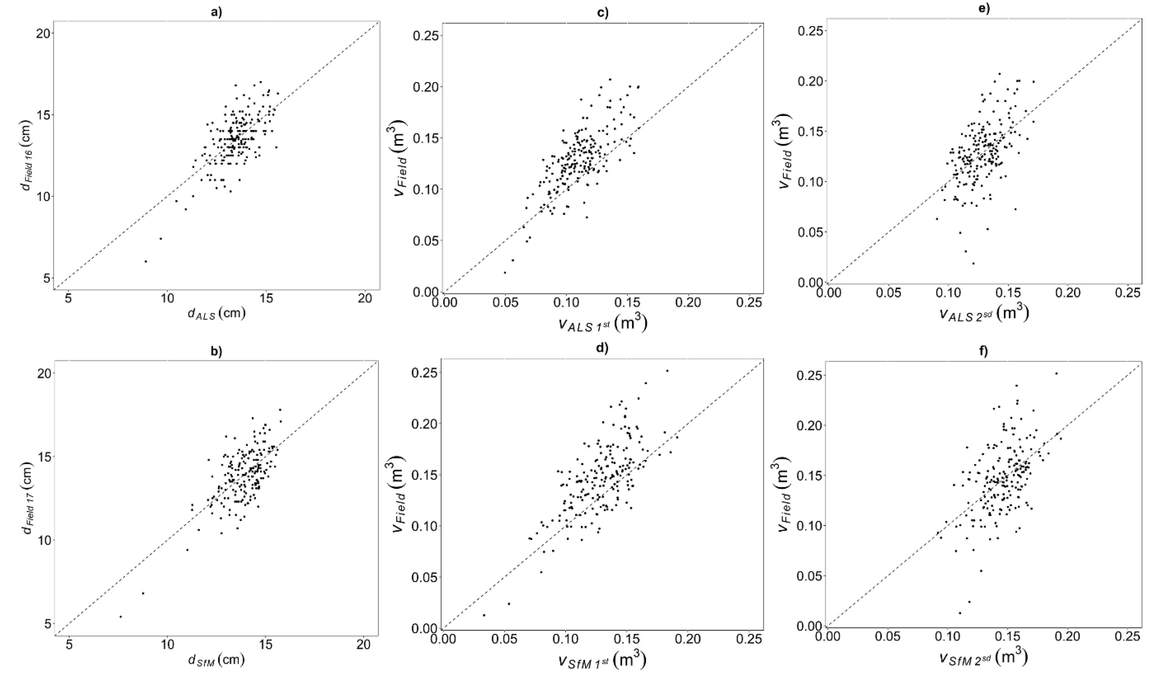
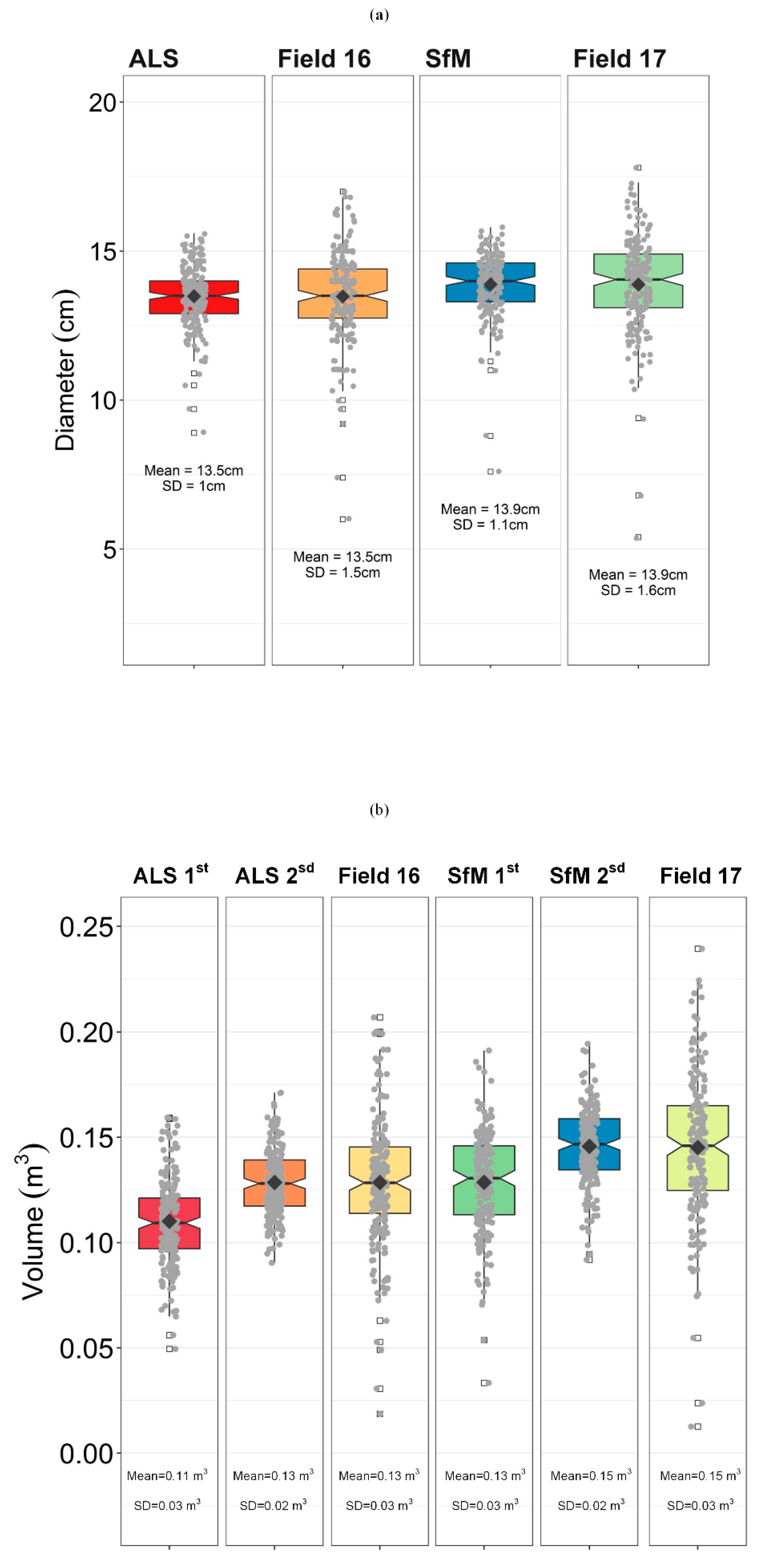
Field, ALS and SfM Volume Estimation

Table 2. Models selected for estimating SfM and ALS derived individual tree diameter and volume.

Approach	Dependent variable	Predictors	Parameter estimate	Standard error	p-value	Mef	RMSE (cm)	rRMSE (%)	bias (cm)
1st	dSfM	Constant	0.863	1.170	< 0.001	0.45	1.17	8.49	0.38
		hSfM	0.907	0.108	< 0.001
		caSfM	0.037	0.037	0.013
	dALS	Constant	0.564	0.151	< 0.001	0.47	1.12	8.31	0.35
		hALS	1.042	0.090	< 0.001
		caALS	0.062	0.015	< 0.001
Approach	Dependent variable	Predictors	Parameter estimate	Standard error	p-value	Mef	RMSE (m3)	rRMSE (%)	bias (m3)
2nd	vSfM	Constant	0.004	0.002	0.082	0.43	0.030	20.31	0.0016
		hSfM	1.192	0.201	< 0.001
		caSfM	0.151	0.035	< 0.001
	vALS	Constant	0.001	0.000	0.106	0.46	0.026	19.97	0.0004
		hALS	1.828	0.224	< 0.001
		caALS	0.024	0.037	< 0.001

h_SfM and h_ALS are the SfM and ALS-derived tree height (m), ca_SfM and ca_ALS are the SfM and ALS-derived individual crown area (m²), Mef is the model efficiency statistic, RMSE is the root mean squared error and rRMSE is the relative root mean square error.

shows the parameter estimates and goodness-of-fit statistics for the models used to predict d (cm) in the first approach, and v directly estimated by SfM- and ALS-variables in the second approach.

In the first approach, non-linear regression yielded an Mef value of 0.45 for the SfM-estimated diameter and 0.47 for ALS-estimated diameter (RMSE = 1.17 and 1.12 cm, rRMSE of 8.49 % and 8.31%, respectively). Although the UAV-based DAP method tends to underestimate tree height relative to field measurements (hypsometers), there was no appreciable bias throughout the observed diameter (Figure 5a,b). The bias values (0.38 and 0.35 cm) indicated a slight tendency to overestimate the initial diameter values from field data (Figure 5a,b). On the other hand, although d was not directly measured in CHMs derived from UAV and ALS, h_SfM and h_ALS were, and these variables were significant in the SfM and ALS equations. For d_SfM and d_ALS modelling, the crown area (ca_SfM and ca_ALS) was also statistically significant (p < 0.05 and p < 0.001, respectively).

In the case of v_ALS modelling, the second approach yielded an Mef value of 0.56. The mean rRMSE of v estimation was 20.31% (0.030 m³) when calculated on the basis of the SfM cloud, and 19.97% (0.026 m³) when based on the ALS cloud. There were no appreciable biases from the models throughout the observed volume range using both approaches (Figure 5c–f). However, the tendency of ALS and SfM to underestimate h may be the main reason for the slight underestimation of v in the first approach (Figure 5c,d). In the case of the second approach, a slightly positive bias (0.0004 and 0.0016 m³) indicated slight overestimation when volume was modeled directly form ALS- and SfM-variables (Figure 5e,f).

The t-test (

Table 3. Field, ALS and SfM diameter and volume estimations from both approaches with their minimum (Min.), mean (Mean), maximum (Max.) and standard deviation (SD) values and the results for the t-test in the subsample of 192 trees for SfM and 199 for ALS, respectively. Field 16 and Field 17 are the field data acquisition years for ALS (Dec 2016) and SfM (Sep 2017), respectively.

Plot	dALS (cm)		dSfM (cm)		vALS (m3)			vSfM (m3)
	ALS	Field 16	SfM	Field 17	ALS 1st	ALS 2sd	Field 16	SfM 1st	SfM 2sd	Field 17
P1	14.1	13.3	14.3	13.4	0.13	0.15	0.13	0.15	0.15	0.14
P2	13.4	12.5	14.0	13.4	0.11	0.14	0.11	0.13	0.15	0.14
P3	13.1	13.3	13.9	14.0	0.10	0.13	0.12	0.12	0.14	0.15
P4	13.4	13.8	13.8	14.3	0.11	0.14	0.13	0.12	0.14	0.15
P5	13.5	13.8	14.0	14.2	0.11	0.14	0.13	0.13	0.15	0.15
P6	13.2	14.2	13.1	14.0	0.11	0.16	0.14	0.12	0.14	0.14
Min.	8.9	6.0	7.6	5.4	0.05	0.05	0.02	0.03	0.09	0.01
Mean	13.5	13.5	13.9	13.9	0.11	0.15	0.13	0.13	0.15	0.15
Max.	15.6	17.0	15.8	17.8	0.16	0.20	0.21	0.19	0.19	0.25
SD	1.0	1.5	1.1	1.6	0.02	0.02	0.03	0.02	0.02	0.03
t-test p-value	0.98		0.98		<0.001	0.99		<0.001	0.98

) showed that there were no evidence of significant differences between observed and estimated values of diameter (p-values of 0.98 for both approaches in the subsample of 192 trees for SfM and 199 for ALS, respectively) and volume using the second approach (p-values of 0.99 for ALS and 0.98 for SfM, Figure 6b). However, there were significant differences using the 1st approach between the observed values and estimated value at the tree level (Table 3, Figure 6b). It is important to note that the mean values of field data for diameter and volume computed for ALS and SfM in the subsample were similar that the values considering the 6 field plots for the total of 323 reference trees, except for the mean volume values for volume in 2017 (Table 3).

4. Discussion

Both v_SfM and v_ALS were accurately estimated from UAV photograph and ALS-based 3-D point clouds using SfM- and ALS-variables extracted automatically from their respective CHMs. Although ALS-based methods and UAV-based DAP methods tend to underestimate tree height [73,74,77], relative to field measurements (hypsometers), no appreciable biases in the observed diameter and volume range estimations occurred with either technologies in the 2nd approach.

Variables derived from the automated processing of ALS and UAV-based DAP with ITC delineation (h_SfM, h_ALS, ca_SfM, and ca_ALS) were found to be significant explanatory variables for predicting d and v in both approaches; however, the Mef and RMSE values for diameter models indicate poorer fits than reported in some recent studies in P. pinea plantations [57] (Mef = 0.79, rRMSE = 4.99%, n = 50 trees) and Japanese Cypress (Chamaecyparis obtusa) [84] (R² = 0.79, n = 51 individual trees where d ranged from 11 to 58 cm) using UAV-based DAP point clouds.

In the case of ALS-based diameter models, our results were similar in terms of R² to those reported by Chisholm et al. [85], who extracted forest below-canopy information using UAV-based LiDAR and developed post-processing software to detect trees and to estimate their diameters (R² = 0.45, rRMSE = 25.1%). Finally, the results were also similar in terms of rRMSE to those reported by Cosenza et al. [86] in a eucalyptus plantation in Brazil (rRMSE = 9%), for an exponential equation with h as explanatory variable. Cosenza et al. [86] also observed a slight tendency to overestimate the initial diameter values (bias = 0.12 cm).

Studies conducted in Picea abies (L.) H. Karst. and Pinus sylvestris L. stands in Sweden and in Pinus taeda L. stands in the SE United States found that ALS-derived h and crown diameter (cd) explained up to 87% and 91% of the variance associated with the estimation of d, with RMSE of 3.8 and 4.9 cm, respectively [87,88]. Zhao et al. [89] reported an R² value of 0.87 and a RMSE value of 5.2 cm for ALS-derived tree dimension variables including h, cd and crown base height in P. taeda stands. In this study, the diameter equation based on ALS-derived variables performed well, although the values of Mef were slightly lower than some of those reported for other species [87,88].

Regarding volume modelling, the performance of the v_ALS and v_SfM estimates for predicting tree volume directly from ALS- and SfM-derived variables (the second approach, R² = 0.46, R² = 0.43; RMSE = 0.026 m³, RMSE = 0.030 m³; respectively) was lower than that obtained in different conifer species (R² = 0.88) [88], as well as in P. taeda (R² = 0.80) [89] and P. pinea (Mef = 0.84 − 0.85) [57]. The mean differences between the deviations of field volume and the ALS- or SfM-derived volume were statistically significant using the 1st approach. The tendency of ALS and UAV-based DAP technologies to underestimate h may be the main reason for the underestimation of v with 1st approach. It should be also borne in mind that the ALS and UAV-based DAP, as a tree height estimation technique, tends to underestimate tree height (e.g., DAP [39,90,91], UAV-based DAP [47,74,76,92] and ALS [73,77,93,94,95] point cloud data). However, our volume modelling results suggest that this bias may not influence in volume estimations using the 2nd approach, leaving open the question as to when and where specific models should be developed for correcting the bias at tree level depending on particular species or forest structure [77]. The results of this study are consistent with the approaches used by other authors [57,73], in which the use of linear regression improved the accuracy of tree height estimations from DAP-ALS data in terms of RMSE and bias, instead of using tree height extracted directly from the CHM to calculate the RMSEs and bias [74], as also occurred with modelling volume in the present study.

There are three possible reasons for the differences in performance for diameter models using SfM- and ALS-variables relative to other species: (i) First, broadleaved trees trees in particular are more challenging for both local maxima detection and delineation compared to conifer trees. (ii) Second, crown delineation remains difficult because the crowns of neighboring trees often overlap due to the high density of trees per unit area. (iii) Third, the low density of leaves in the crowns and the small size of the crowns of mature trees prevent a considerable number of laser pulses from hitting the crown (thus hampering crown delineation). As expected, the ALS cloud contributed to yielding slightly better results for diameter and volume estimation, but we did not observe differences in terms of volume estimations. As with previous studies using DAP, ITC delineation is more affected than ALS crown delineation as UAV-based DAP has several limitations: (i) ALS is insensitive to shadows made by clouds [15], (ii) the images are strongly influenced by atmospheric conditions (e.g., wind swaying can cause problems building point clouds), solar illumination and view angles (sun, surface and sensor geometry), occlusions caused by shadows are particular problematic for generation of image-based point clouds in dense forest canopies [45,96,97,98]. In addition, seasonality (timing) influences underestimation of tree heights but can improve detection accuracy [99]. The allometric relationship between volume and ALS or SfM crown-derived variables could be also refined through improvements in UAV imagery acquisition and processing.

Finally, a more comprehensive examination of the effects of varying the conditions of UAV-based DAP acquisition and their implications for estimating forest inventory variables in different types of forest should be carried out using these techniques [100,101,102]. Many facets have not been explored with current state-of-the-art techniques. Several effects related to flight configuration (i.e., flight speed, wind effect, illumination effect), post-processing pipelines (i.e., comparing different SfM algorithms), field data collection (i.e., number of field plots) and environmental variables (i.e., effect of aspect or slope when using different DEM approaches or the DEM-independent approach) must be analyzed. Future research must also explore how the type of platform (fixed-wing versus multirotor), sensors or the type of forest (e.g., temperate, deciduous, evergreen needleleaf, and tropical forest) influence the ability of UAV-based DAP methods to accurately characterize biometric tree variables at the tree level.

5. Conclusions

The study findings showed that UAV-based DAP methods are useful and comparable to ALS for forest inventory and sustainable forest management in planted forests, by providing accurate estimations of forest structural attributes at the tree level. The results suggested that object-based image analysis (OBIA) provides more accurate predictive models for individual volumes of Eucalyptus trees based on ALS-derived and SfM-derived variables from the 3D point clouds than those obtained using indirect approaches to estimate diameter.

References

1. Burkhart, H.E.; Tomé, M. Modeling Forest Trees and Stands; Springer Science & Business Media: Dordrecht, The Netherlands, 2012. [Google Scholar]
2. Bauwens, S.; Bartholomeus, H.; Calders, K.; Lejeune, P. Forest Inventory with Terrestrial LiDAR: A Comparison of Static and Hand-Held Mobile Laser Scanning. Forests 2016, 7, 127. [Google Scholar] [CrossRef]
3. Williams, M.S.; Bechtold, W.A.; LaBau, V.J. Five Instruments for Measuring Tree Height: An Evaluation. South. J. Appl. For. 1994, 18, 76–82. [Google Scholar] [CrossRef] [Green Version]
4. Thenkabail, P.S.; Durrieu, S.; Véga, C.; Bouvier, M.; Gosselin, F.; Renaud, J.-P.; Saint-André, L. Optical Remote Sensing of Tree and Stand Heights. In Land Resources Monitoring, Modeling, and Mapping with Remote Sensing; CRC Press: Boca Raton, FL, USA, 2015; pp. 449–485. [Google Scholar]
5. Díaz-Varela, R.A.; de la Rosa, R.; León, L.; Zarco-Tejada, P.J. High-Resolution Airborne UAV Imagery to Assess Olive Tree Crown Parameters Using 3D Photo Reconstruction: Application in Breeding Trials. Remote Sens. 2015, 7, 4213–4232. [Google Scholar] [CrossRef] [Green Version]
6. Panagiotidis, D.; Abdollahnejad, A.; Surový, P.; Chiteculo, V. Determining Tree Height and Crown Diameter from High-Resolution UAV Imagery. Int. J. Remote Sens. 2016, 1–19. [Google Scholar] [CrossRef]
7. White, J.C.; Coops, N.C.; Wulder, M.A.; Vastaranta, M.; Hilker, T.; Tompalski, P. Remote Sensing Technologies for Enhancing Forest Inventories: A Review. Can. J. Remote Sens. 2016, 1–23. [Google Scholar] [CrossRef]
8. Giannetti, F.; Puletti, N.; Quatrini, V.; Travaglini, D.; Bottalico, F.; Corona, P.; Chirici, G. Integrating Terrestrial and Airborne Laser Scanning for the Assessment of Single-Tree Attributes in Mediterranean Forest Stands. Eur. J. Remote Sens. 2018, 51, 795–807. [Google Scholar] [CrossRef]
9. Liang, X.; Kankare, V.; Hyyppä, J.; Wang, Y.; Kukko, A.; Haggrén, H.; Yu, X.; Kaartinen, H.; Jaakkola, A.; Guan, F. Terrestrial Laser Scanning in Forest Inventories. ISPRS J. Photogramm. Remote Sens. 2016, 115, 63–77. [Google Scholar] [CrossRef]
10. Abegg, M.; Kükenbrink, D.; Zell, J.; Schaepman, M.E.; Morsdorf, F. Terrestrial Laser Scanning for Forest Inventories—Tree Diameter Distribution and Scanner Location Impact on Occlusion. Forests 2017, 8, 184. [Google Scholar] [CrossRef]
11. Liu, G.; Wang, J.; Dong, P.; Chen, Y.; Liu, Z. Estimating Individual Tree Height and Diameter at Breast Height (DBH) from Terrestrial Laser Scanning (TLS) Data at Plot Level. Forests 2018, 9, 398. [Google Scholar] [CrossRef]
12. Baltsavias, E.P. A Comparison between Photogrammetry and Laser Scanning. ISPRS J. Photogramm. Remote Sens. 1999, 54, 83–94. [Google Scholar] [CrossRef]
13. Næsset, E. Determination of Mean Tree Height of Forest Stands by Digital Photogrammetry. Scand. J. For. Res. 2002, 17, 446–459. [Google Scholar] [CrossRef]
14. Næsset, E. Predicting Forest Stand Characteristics with Airborne Scanning Laser Using a Practical Two-Stage Procedure and Field Data. Remote Sens. Environ. 2002, 80, 88–99. [Google Scholar] [CrossRef]
15. White, J.; Wulder, M.; Vastaranta, M.; Coops, N.; Pitt, D.; Woods, M. The Utility of Image-Based Point Clouds for Forest Inventory: A Comparison with Airborne Laser Scanning. Forests 2013, 4, 518–536. [Google Scholar] [CrossRef] [Green Version]
16. Fritz, A.; Kattenborn, T.; Koch, B. UAV-Based Photogrammetric Point Clouds—Tree Stem Mapping in Open Stands in Comparison to Terrestrial Laser Scanner Point Clouds. Int. Arch. Photogramm. Remote Sens. Spat. Inf. Sci. 2013, 40, 141–146. [Google Scholar] [CrossRef]
17. Gobakken, T.; Bollandsås, O.M.; Næsset, E. Comparing Biophysical Forest Characteristics Estimated from Photogrammetric Matching of Aerial Images and Airborne Laser Scanning Data. Scand. J. For. Res. 2015, 30, 73–86. [Google Scholar] [CrossRef]
18. Maltamo, M.; Næsset, E.; Vauhkonen, J. Forestry Applications of Airborne Laser Scanning. Concepts Case Stud. Manag. Ecosys 2014, 27, 2014. [Google Scholar]
19. Naesset, E. Estimating Timber Volume of Forest Stands Using Airborne Laser Scanner Data. Remote Sens. Environ. 1997, 61, 246–253. [Google Scholar] [CrossRef]
20. Hyyppä, J.; Hyyppä, H.; Leckie, D.; Gougeon, F.; Yu, X.; Maltamo, M. Review of Methods of Small-Footprint Airborne Laser Scanning for Extracting Forest Inventory Data in Boreal Forests. Int. J. Remote Sens. 2008, 29, 1339–1366. [Google Scholar] [CrossRef]
21. Van Leeuwen, M.; Nieuwenhuis, M. Retrieval of Forest Structural Parameters Using LiDAR Remote Sensing. Eur. J. For. Res. 2010, 129, 749–770. [Google Scholar] [CrossRef]
22. Puliti, S.; Gobakken, T.; Ørka, H.O.; Næsset, E. Assessing 3D Point Clouds from Aerial Photographs for Species-Specific Forest Inventories. Scand. J. For. Res. 2017, 32, 68–79. [Google Scholar] [CrossRef]
23. Tuominen, S.; Balazs, A.; Saari, H.; Pölönen, I.; Sarkeala, J.; Viitala, R. Unmanned Aerial System Imagery and Photogrammetric Canopy Height Data in Area-Based Estimation of Forest Variables. Silva Fenn. 2015, 49. [Google Scholar] [CrossRef]
24. Bohlin, J.; Wallerman, J.; Fransson, J.E. Forest Variable Estimation Using Photogrammetric Matching of Digital Aerial Images in Combination with a High-Resolution DEM. Scand. J. For. Res. 2012, 27, 692–699. [Google Scholar] [CrossRef]
25. Nurminen, K.; Karjalainen, M.; Yu, X.; Hyyppä, J.; Honkavaara, E. Performance of Dense Digital Surface Models Based on Image Matching in the Estimation of Plot-Level Forest Variables. ISPRS J. Photogramm. Remote Sens. 2013, 83, 104–115. [Google Scholar] [CrossRef]
26. St-Onge, B.; Vega, C.; Fournier, R.A.; Hu, Y. Mapping Canopy Height Using a Combination of Digital Stereo-photogrammetry and Lidar. Int. J. Remote Sens. 2008, 29, 3343–3364. [Google Scholar] [CrossRef]
27. Zarco-Tejada, P.J.; Diaz-Varela, R.; Angileri, V.; Loudjani, P. Tree Height Quantification Using Very High Resolution Imagery Acquired from an Unmanned Aerial Vehicle (UAV) and Automatic 3D Photo-Reconstruction Methods. Eur. J. Agron. 2014, 55, 89–99. [Google Scholar] [CrossRef]
28. Goodbody, T.R.; Coops, N.C.; White, J.C. Digital Aerial Photogrammetry for Updating Area-Based Forest Inventories: A Review of Opportunities, Challenges, and Future Directions. Curr. For. Rep. 2019, 5, 55–75. [Google Scholar] [CrossRef] [Green Version]
29. Iglhaut, J.; Cabo, C.; Puliti, S.; Piermattei, L.; O’Connor, J.; Rosette, J. Structure from Motion Photogrammetry in Forestry: A Review. Curr. For. Rep. 2019, 1–14. [Google Scholar] [CrossRef]
30. White, J.C.; Stepper, C.; Tompalski, P.; Coops, N.C.; Wulder, M.A. Comparing ALS and Image-Based Point Cloud Metrics and Modelled Forest Inventory Attributes in a Complex Coastal Forest Environment. Forests 2015, 6, 3704–3732. [Google Scholar] [CrossRef]
31. Baltsavias, E.; Gruen, A.; Eisenbeiss, H.; Zhang, L.; Waser, L.T. High-quality Image Matching and Automated Generation of 3D Tree Models. Int. J. Remote Sens. 2008, 29, 1243–1259. [Google Scholar] [CrossRef]
32. Véga, C.; St-Onge, B. Height Growth Reconstruction of a Boreal Forest Canopy over a Period of 58 Years Using a Combination of Photogrammetric and Lidar Models. Remote Sens. Environ. 2008, 112, 1784–1794. [Google Scholar] [CrossRef]
33. Waser, L.T.; Baltsavias, E.; Ecker, K.; Eisenbeiss, H.; Feldmeyer-Christe, E.; Ginzler, C.; Küchler, M.; Zhang, L. Assessing Changes of Forest Area and Shrub Encroachment in a Mire Ecosystem Using Digital Surface Models and CIR Aerial Images. Remote Sens. Environ. 2008, 112, 1956–1968. [Google Scholar] [CrossRef]
34. Vastaranta, M.; Wulder, M.A.; White, J.C.; Pekkarinen, A.; Tuominen, S.; Ginzler, C.; Kankare, V.; Holopainen, M.; Hyyppä, J.; Hyyppä, H. Airborne Laser Scanning and Digital Stereo Imagery Measures of Forest Structure: Comparative Results and Implications to Forest Mapping and Inventory Update. Can. J. Remote Sens. 2013, 39, 382–395. [Google Scholar] [CrossRef]
35. Pitt, D.G.; Woods, M.; Penner, M. A Comparison of Point Clouds Derived from Stereo Imagery and Airborne Laser Scanning for the Area-Based Estimation of Forest Inventory Attributes in Boreal Ontario. Can. J. Remote Sens. 2014, 40, 214–232. [Google Scholar] [CrossRef]
36. Rahlf, J.; Breidenbach, J.; Solberg, S.; Næsset, E.; Astrup, R. Comparison of Four Types of 3D Data for Timber Volume Estimation. Remote Sens. Environ. 2014, 155, 325–333. [Google Scholar] [CrossRef]
37. Ota, T.; Ogawa, M.; Shimizu, K.; Kajisa, T.; Mizoue, N.; Yoshida, S.; Takao, G.; Hirata, Y.; Furuya, N.; Sano, T. Aboveground Biomass Estimation Using Structure from Motion Approach with Aerial Photographs in a Seasonal Tropical Forest. Forests 2015, 6, 3882–3898. [Google Scholar] [CrossRef] [Green Version]
38. Holopainen, M.; Vastaranta, M.; Karjalainen, M.; Karila, K.; Kaasalainen, S.; Honkavaara, E.; Hyyppä, J. Forest Inventory Attribute Estimation Using Airborne Laser Scanning, Aerial Stereo Imagery, Radargrammetry and Interferometry-Finnish Experiences of the 3D Techniques. ISPRS Ann. Photogramm. Remote Sens. Spat. Inf. Sci. 2015, 2, 63. [Google Scholar] [CrossRef]
39. Tanhuanpää, T.; Saarinen, N.; Kankare, V.; Nurminen, K.; Vastaranta, M.; Honkavaara, E.; Karjalainen, M.; Yu, X.; Holopainen, M.; Hyyppä, J. Evaluating the Performance of High-Altitude Aerial Image-Based Digital Surface Models in Detecting Individual Tree Crowns in Mature Boreal Forests. Forests 2016, 7, 143. [Google Scholar] [CrossRef]
40. Wallace, L.; Lucieer, A.; Watson, C.; Turner, C. Assessing the Feasibility of UAV-Based LiDAR for High Resolution Forest Change Detection. Proc. ISPRS—Int. Arch. Photogramm. Remote Sens. Spat. Inf. Sci. 2012, 39, B7. [Google Scholar] [CrossRef]
41. Lisein, J.; Pierrot-Deseilligny, M.; Bonnet, S.; Lejeune, P. A Photogrammetric Workflow for the Creation of a Forest Canopy Height Model from Small Unmanned Aerial System Imagery. Forests 2013, 4, 922–944. [Google Scholar] [CrossRef] [Green Version]
42. Wallace, L.; Lucieer, A.; Malenovský, Z.; Turner, D.; Vopěnka, P. Assessment of Forest Structure Using Two UAV Techniques: A Comparison of Airborne Laser Scanning and Structure from Motion (SfM) Point Clouds. Forests 2016, 7, 62. [Google Scholar] [CrossRef]
43. Jaakkola, A.; Hyyppä, J.; Yu, X.; Kukko, A.; Kaartinen, H.; Liang, X.; Hyyppä, H.; Wang, Y. Autonomous Collection of Forest Field Reference—The Outlook and a First Step with UAV Laser Scanning. Remote Sens. 2017, 9, 785. [Google Scholar] [CrossRef]
44. Dandois, J.P.; Ellis, E.C. Remote Sensing of Vegetation Structure Using Computer Vision. Remote Sens. 2010, 2, 1157–1176. [Google Scholar] [CrossRef] [Green Version]
45. Dandois, J.P.; Olano, M.; Ellis, E.C. Optimal Altitude, Overlap, and Weather Conditions for Computer Vision UAV Estimates of Forest Structure. Remote Sens. 2015, 7, 13895–13920. [Google Scholar] [CrossRef] [Green Version]
46. Dandois, J.P.; Ellis, E.C. High Spatial Resolution Three-Dimensional Mapping of Vegetation Spectral Dynamics Using Computer Vision. Remote Sens. Environ. 2013, 136, 259–276. [Google Scholar] [CrossRef]
47. Zahawi, R.A.; Dandois, J.P.; Holl, K.D.; Nadwodny, D.; Reid, J.L.; Ellis, E.C. Using Lightweight Unmanned Aerial Vehicles to Monitor Tropical Forest Recovery. Biol. Conserv. 2015, 186, 287–295. [Google Scholar] [CrossRef]
48. Guerra-Hérnandez, J.; González-Ferreiro, E.; Sarmento, A.; Silva, J.; Nunes, A.; Correia, A.C.; Fontes, L.; Tomé, M.; Díaz-Varela, R. Short Communication. Using High Resolution UAV Imagery to Estimate Tree Variables in Pinus Pinea Plantation in Portugal. For. Syst. 2016, 25, 9. [Google Scholar] [CrossRef]
49. Mohan, M.; Silva, C.A.; Klauberg, C.; Jat, P.; Catts, G.; Cardil, A.; Hudak, A.T.; Dia, M. Individual Tree Detection from Unmanned Aerial Vehicle (UAV) Derived Canopy Height Model in an Open Canopy Mixed Conifer Forest. Forests 2017, 8, 340. [Google Scholar] [CrossRef]
50. Thiel, C.; Schmullius, C. Comparison of UAV Photograph-Based and Airborne Lidar-Based Point Clouds over Forest from a Forestry Application Perspective. Int. J. Remote Sens. 2017, 38, 2411–2426. [Google Scholar] [CrossRef]
51. Cardil, A.; Vepakomma, U.; Brotons, L. Assessing Pine Processionary Moth Defoliation Using Unmanned Aerial Systems. Forests 2017, 8, 402. [Google Scholar] [CrossRef]
52. Navarro, J.; Algeet, N.; Fernández-Landa, A.; Esteban, J.; Rodríguez-Noriega, P.; Guillén-Climent, M. Integration of UAV, Sentinel-1, and Sentinel-2 Data for Mangrove Plantation Aboveground Biomass Monitoring in Senegal. Remote Sens. 2019, 11, 77. [Google Scholar] [CrossRef]
53. Puliti, S.; Ørka, H.O.; Gobakken, T.; Næsset, E. Inventory of Small Forest Areas Using an Unmanned Aerial System. Remote Sens. 2015, 7, 9632–9654. [Google Scholar] [CrossRef] [Green Version]
54. Torresan, C.; Berton, A.; Carotenuto, F.; Di Gennaro, S.F.; Gioli, B.; Matese, A.; Miglietta, F.; Vagnoli, C.; Zaldei, A.; Wallace, L. Forestry Applications of UAVs in Europe: A Review. Int. J. Remote Sens. 2017, 38, 2427–2447. [Google Scholar] [CrossRef]
55. Whitehead, K.; Hugenholtz, C.H. Remote Sensing of the Environment with Small Unmanned Aircraft Systems (UASs), Part 1: A Review of Progress and Challenges 1. J. Unmanned Veh. Syst. 2014, 2, 69–85. [Google Scholar] [CrossRef]
56. Tang, L.; Shao, G. Drone Remote Sensing for Forestry Research and Practices. J. For. Res. 2015, 1–7. [Google Scholar] [CrossRef]
57. Guerra-Hernández, J.; González-Ferreiro, E.; Monleón, V.; Faias, S.; Tomé, M.; Díaz-Varela, R. Use of Multi-Temporal UAV-Derived Imagery for Estimating Individual Tree Growth in Pinus Pinea Stands. Forests 2017, 8, 300. [Google Scholar] [CrossRef]
58. Pádua, L.; Hruška, J.; Bessa, J.; Adão, T.; Martins, L.M.; Gonçalves, J.A.; Peres, E.; Sousa, A.M.; Castro, J.P.; Sousa, J.J. Multi-Temporal Analysis of Forestry and Coastal Environments Using UASs. Remote Sens. 2017, 10, 24. [Google Scholar] [CrossRef]
59. Hall, S.A.; Burke, I.C.; Box, D.O.; Kaufmann, M.R.; Stoker, J.M. Estimating Stand Structure Using Discrete-Return Lidar: An Example from Low Density, Fire Prone Ponderosa Pine Forests. For. Ecol. Manag. 2005, 208, 189–209. [Google Scholar] [CrossRef]
60. Järnstedt, J.; Pekkarinen, A.; Tuominen, S.; Ginzler, C.; Holopainen, M.; Viitala, R. Forest Variable Estimation Using a High-Resolution Digital Surface Model. ISPRS J. Photogramm. Remote Sens. 2012, 74, 78–84. [Google Scholar] [CrossRef]
61. González-Ferreiro, E.; Diéguez-Aranda, U.; Miranda, D. Estimation of Stand Variables in Pinus Radiata D. Don Plantations Using Different LiDAR Pulse Densities. Forestry 2012, 85, 281–292. [Google Scholar] [CrossRef]
62. González-Ferreiro, E.; Diéguez-Aranda, U.; Crecente-Campo, F.; Barreiro-Fernández, L.; Miranda, D.; Castedo-Dorado, F. Modelling Canopy Fuel Variables for Pinus Radiata D. Don in NW Spain with Low-Density LiDAR Data. Int. J. Wildland Fire 2014, 23, 350–362. [Google Scholar] [CrossRef]
63. Montaghi, A.; Corona, P.; Dalponte, M.; Gianelle, D.; Chirici, G.; Olsson, H. Airborne Laser Scanning of Forest Resources: An Overview of Research in Italy as a Commentary Case Study. Int. J. Appl. Earth Obs. Geoinformation 2013, 23, 288–300. [Google Scholar] [CrossRef]
64. Corona, P.; Cartisano, R.; Salvati, R.; Chirici, G.; Floris, A.; Di Martino, P.; Marchetti, M.; Scrinzi, G.; Clementel, F.; Torresan, C. Airborne Laser Scanning to Support Forest Resource Management under Alpine, Temperate and Mediterranean Environments in Italy. Eur. J. Remote Sens. 2012, 45, 27–37. [Google Scholar]
65. González-Olabarria, J.-R.; Rodríguez, F.; Fernández-Landa, A.; Mola-Yudego, B. Mapping Fire Risk in the Model Forest of Urbión (Spain) Based on Airborne LiDAR Measurements. For. Ecol. Manag. 2012, 282, 149–156. [Google Scholar] [CrossRef]
66. Guerra-Hernández, J.; Görgens, E.B.; García-Gutiérrez, J.; Rodriguez, L.C.E.; Tomé, M.; González-Ferreiro, E. Comparison of ALS Based Models for Estimating Aboveground Biomass in Three Types of Mediterranean Forest. Eur. J. Remote Sens. 2016, 49, 185–204. [Google Scholar] [CrossRef]
67. Montealegre, A.L.; Lamelas, M.T.; Tanase, M.A.; de la Riva, J. Estimación de La Severidad En Incendios Forestales a Partir de Datos LiDAR-PNOA y Valores de Composite Burn Index. Rev. Teledetec. 2017, 49, 1–16. [Google Scholar] [CrossRef]
68. Montealegre, A.L.; Lamelas, M.T.; de la Riva, J.; García-Martín, A.; Escribano, F. Use of Low Point Density ALS Data to Estimate Stand-Level Structural Variables in Mediterranean Aleppo Pine Forest. For. Int. J. For. Res. 2016, 89, 373–382. [Google Scholar] [CrossRef]
69. Domingo, D.; Alonso, R.; Lamelas, M.T.; Montealegre, A.L.; Rodríguez, F.; de la Riva, J. Temporal Transferability of Pine Forest Attributes Modeling Using Low-Density Airborne Laser Scanning Data. Remote Sens. 2019, 11, 261. [Google Scholar] [CrossRef]
70. Silva, C.A.; Klauberg, C.; Hudak, A.T.; Vierling, L.A.; Liesenberg, V.; Carvalho, S.P.E.; Rodriguez, L.C. A Principal Component Approach for Predicting the Stem Volume in Eucalyptus Plantations in Brazil Using Airborne LiDAR Data. For. Int. J. For. Res. 2016, 89, 422–433. [Google Scholar] [CrossRef]
71. Kachamba, D.J.; Ørka, H.O.; Gobakken, T.; Eid, T.; Mwase, W. Biomass Estimation Using 3D Data from Unmanned Aerial Vehicle Imagery in a Tropical Woodland. Remote Sens. 2016, 8, 968. [Google Scholar] [CrossRef]
72. St-Onge, B.; Audet, F.-A.; Bégin, J. Characterizing the Height Structure and Composition of a Boreal Forest Using an Individual Tree Crown Approach Applied to Photogrammetric Point Clouds. Forests 2015, 6, 3899–3922. [Google Scholar] [CrossRef]
73. Mielcarek, M.; Stereńczak, K.; Khosravipour, A. Testing and Evaluating Different LiDAR-Derived Canopy Height Model Generation Methods for Tree Height Estimation. Int. J. Appl. Earth Obs. Geoinformation 2018, 71, 132–143. [Google Scholar] [CrossRef]
74. Guerra-Hernández, J.; Cosenza, D.N.; Rodriguez, L.C.E.; Silva, M.; Tomé, M.; Díaz-Varela, R.A.; González-Ferreiro, E. Comparison of ALS-and UAV (SfM)-Derived High-Density Point Clouds for Individual Tree Detection in Eucalyptus Plantations. Int. J. Remote Sens. 2018, 39, 5211–5235. [Google Scholar]
75. Maltamo, M.; Eerikäinen, K.; Packalén, P.; Hyyppä, J. Estimation of Stem Volume Using Laser Scanning-Based Canopy Height Metrics. Forestry 2006, 79, 217–229. [Google Scholar] [CrossRef]
76. Hentz, Â.M.; Silva, C.A.; Dalla Corte, A.P.; Netto, S.P.; Strager, M.P.; Klauberg, C. Estimating Forest Uniformity in Eucalyptus Spp. and Pinus Taeda L. Stands Using Field Measurements and Structure from Motion Point Clouds Generated from Unmanned Aerial Vehicle (UAV) Data Collection. For. Syst. 2018, 27, 5. [Google Scholar] [CrossRef]
77. Roussel, J.-R.; Caspersen, J.; Béland, M.; Thomas, S.; Achim, A. Removing Bias from LiDAR-Based Estimates of Canopy Height: Accounting for the Effects of Pulse Density and Footprint Size. Remote Sens. Environ. 2017, 198, 1–16. [Google Scholar] [CrossRef]
78. Tomé, M.; Tomé, J.; Ribeiro, F.; Faias, S. Equações de Volume Total, Volume Percentual e de Perfil Do Tronco Para Eucalyptus Globulus Labill. Em Portugal. Silva Lusit. 2007, 15, 25–39. [Google Scholar]
79. McGaughey, R.J. FUSION/LDV: Software for LIDAR Data Analysis and Visualization; Version 3.60+; Pacific Northwest Research Station, United States Department of Agriculture Forest Service: Seattle, WA, USA, 2017.
80. Isenburg, M. LAStools—Efficient Tools for LiDAR Processing; Version 160921; Academic: Cambridge, MA, USA, 2016. [Google Scholar]
81. González-Ferreiro, E.; Diéguez-Aranda, U.; Barreiro-Fernández, L.; Buján, S.; Barbosa, M.; Suárez, J.C.; Bye, I.J.; Miranda, D. A Mixed Pixel-and Region-Based Approach for Using Airborne Laser Scanning Data for Individual Tree Crown Delineation in Pinus Radiata D. Don Plantations. Int. J. Remote Sens. 2013, 34, 7671–7690. [Google Scholar] [CrossRef]
82. Vanclay, J.K.; Skovsgaard, J.P. Evaluating Forest Growth Models. Ecol. Model. 1997, 98, 1–12. [Google Scholar] [CrossRef]
83. Shapiro, S.S.; Wilk, M.B.; Chen, H.J. A Comparative Study of Various Tests for Normality. J. Am. Stat. Assoc. 1968, 63, 1343–1372. [Google Scholar] [CrossRef]
84. Iizuka, K.; Yonehara, T.; Itoh, M.; Kosugi, Y. Estimating Tree Height and Diameter at Breast Height (DBH) from Digital Surface Models and Orthophotos Obtained with an Unmanned Aerial System for a Japanese Cypress (Chamaecyparis Obtusa) Forest. Remote Sens. 2017, 10, 13. [Google Scholar] [CrossRef]
85. Chisholm, R.A.; Cui, J.; Lum, S.K.; Chen, B.M. UAV LiDAR for Below-Canopy Forest Surveys. J. Unmanned Veh. Syst. 2013, 1, 61–68. [Google Scholar] [CrossRef]
86. Cosenza, D.N.; Soares, V.P.; Leite, H.G.; Gleriani, J.M.; do Amaral, C.H.; Gripp Júnior, J.; da Silva, A.A.L.; Soares, P.; Tomé, M. Airborne Laser Scanning Applied to Eucalyptus Stand Inventory at Individual Tree Level. Pesqui. Agropecuária Bras. 2018, 53, 1373–1382. [Google Scholar] [CrossRef]
87. Persson, A.; Holmgren, J.; Söderman, U. Detecting and Measuring Individual Trees Using an Airborne Laser Scanner. Photogramm. Eng. Remote Sens. 2002, 68, 925–932. [Google Scholar]
88. Popescu, S.C. Estimating Biomass of Individual Pine Trees Using Airborne Lidar. Biomass Bioenergy 2007, 31, 646–655. [Google Scholar] [CrossRef]
89. Zhao, K.; Popescu, S.; Nelson, R. Lidar Remote Sensing of Forest Biomass: A Scale-Invariant Estimation Approach Using Airborne Lasers. Remote Sens. Environ. 2009, 113, 182–196. [Google Scholar] [CrossRef]
90. Korpela, I. Individual Tree Measurements by Means of Digital Aerial Photogrammetry; Finnish Society of Forest Science: Helsinki, Finland, 2004; Volume 3. [Google Scholar]
91. St-Onge, B.; Jumelet, J.; Cobello, M.; Véga, C. Measuring Individual Tree Height Using a Combination of Stereophotogrammetry and Lidar. Can. J. For. Res. 2004, 34, 2122–2130. [Google Scholar] [CrossRef]
92. Jensen, J.L.; Mathews, A.J. Assessment of Image-Based Point Cloud Products to Generate a Bare Earth Surface and Estimate Canopy Heights in a Woodland Ecosystem. Remote Sens. 2016, 8, 50. [Google Scholar] [CrossRef]
93. Hopkinson, C.; Chasmer, L.; Hall, R.J. The Uncertainty in Conifer Plantation Growth Prediction from Multi-Temporal Lidar Datasets. Remote Sens. Environ. 2008, 112, 1168–1180. [Google Scholar] [CrossRef]
94. Yu, X.; Hyyppä, J.; Kukko, A.; Maltamo, M.; Kaartinen, H. Change Detection Techniques for Canopy Height Growth Measurements Using Airborne Laser Scanner Data. Photogramm. Eng. Remote Sens. 2006, 72, 1339–1348. [Google Scholar] [CrossRef]
95. Gatziolis, D.; Fried, J.S.; Monleon, V.S. Challenges to Estimating Tree Height via LiDAR in Closed-Canopy Forests: A Parable from Western Oregon. For. Sci. 2010, 56, 139–155. [Google Scholar]
96. Milas, A.S.; Arend, K.; Mayer, C.; Simonson, M.A.; Mackey, S. Different Colours of Shadows: Classification of UAV Images. Int. J. Remote Sens. 2017, 38, 3084–3100. [Google Scholar] [CrossRef]
97. Laliberte, A.S.; Herrick, J.E.; Rango, A.; Winters, C. Acquisition, Orthorectification, and Object-Based Classification of Unmanned Aerial Vehicle (UAV) Imagery for Rangeland Monitoring. Photogramm. Eng. Remote Sens. 2010, 76, 661–672. [Google Scholar] [CrossRef]
98. Ke, Y.; Quackenbush, L.J. A Review of Methods for Automatic Individual Tree-Crown Detection and Delineation from Passive Remote Sensing. Int. J. Remote Sens. 2011, 32, 4725–4747. [Google Scholar] [CrossRef]
99. Nuijten, R.J.; Coops, N.C.; Goodbody, T.R.; Pelletier, G. Examining the Multi-Seasonal Consistency of Individual Tree Segmentation on Deciduous Stands Using Digital Aerial Photogrammetry (DAP) and Unmanned Aerial Systems (UAS). Remote Sens. 2019, 11, 739. [Google Scholar] [CrossRef]
100. Frey, J.; Kovach, K.; Stemmler, S.; Koch, B. UAV Photogrammetry of Forests as a Vulnerable Process. A Sensitivity Analysis for a Structure from Motion RGB-Image Pipeline. Remote Sens. 2018, 10, 912. [Google Scholar] [CrossRef]
101. Fraser, B.; Congalton, R. Issues in Unmanned Aerial Systems (UAS) Data Collection of Complex Forest Environments. Remote Sens. 2018, 10, 908. [Google Scholar] [CrossRef]
102. Ni, W.; Sun, G.; Pang, Y.; Zhang, Z.; Liu, J.; Yang, A.; Wang, Y.; Zhang, D. Mapping Three-Dimensional Structures of Forest Canopy Using UAV Stereo Imagery: Evaluating Impacts of Forward Overlaps and Image Resolutions With LiDAR Data as Reference. IEEE J. Sel. Top. Appl. Earth Obs. Remote Sens. 2018, 11, 3578–3589. [Google Scholar] [CrossRef]
Figure 1. (a) UAV-derived RGB-orthomosaic image of the study area and 10 ground control points (GCPs) (red dots) (b) UAV-derived Digital Surface Model (DSM) generated using Pix4d® software.
Forests 10 00905 g001
Figure 2. UAV Camera (left) and flight design (right).
Forests 10 00905 g002
Figure 3. Examples of the canopy height models (cool to warm colors representing low to high heights), crown delineation (blue lines), and tree top positions (red dots) within example plots using airborne laser scanning (ALS) (a) and Structure from Motion (SfM) (b).
Forests 10 00905 g003
Figure 4. Summary steps of individual tree crown (ITC) to map volume.
Forests 10 00905 g004
Figure 5. Scatter plots of ALS and SfM-derived variables against field-derived variables: (a) field-measured tree diameter (d) against ALS-estimated tree diameter (dALS); (b) field-measured tree diameter (d) against SfM-estimated tree diameter (dSfM); (c) field-estimated volume (vfield) against ALS-estimated volume (vALS) using the first approach; (d) field-estimated volume (vfield) against SfM-estimated volume (vSfM) using the first approach; (e) field-estimated volume (vfield) against ALS-estimated volume (vALS) using the second approach; (f) field-estimated volume (vfield) against SfM -estimated volume (vSfM) using the second approach.
Forests 10 00905 g005
Figure 6. Box plot of field-measured and remotely sensed estimated values of diameter (a) and volume using the 1st approach and 2nd approach (b). The lower and upper areas of the boxes represent the 5th and 75th percentiles and the horizontal band represents the median. The upper and lower whiskers extend from to the highest and lowest value respectively within the 1.5 times the interquartile range.
Forests 10 00905 g006